On a cross-diffusion system arising in image denosing thanks: Supported by Spanish MCI Project MTM2017-87162-P.

Gonzalo Galiano Dpt. of Mathematics, Universidad de Oviedo, c/ Calvo Sotelo, 33007-Oviedo, Spain (galiano@uniovi.es, julian@uniovi.es)    Julián Velasco22footnotemark: 2
Abstract

We study a generalization of a cross-diffusion problem deduced from a nonlinear complex-variable diffusion model for signal and image denoising.

We prove the existence of weak solutions of the time-independent problem with fidelity terms under mild conditions on the data problem. Then, we show that this translates on the well-posedness of a quasi-steady state approximation of the evolution problem, and also prove the existence of weak solutions of the latter under more restrictive hypothesis.

We finally perform some numerical simulations for image denoising, comparing the performance of the cross-diffusion model to other well-known demoising methods.

Keywords: cross-diffusion, denoising, Perona-Malik, existence of solutions, simulations.

1 Introduction

A fundamental problem in image analysis is the reconstruction of an original image from an observation, usually to perform subsequent operations on it, such as segmentation or inpainting. In this reconstruction, image denoising is the main task, involving the elimination or reduction of random phenomena -noise- which has been introduced in the image acquisition process due to a number of factors like poor lighting, magnetic perturbances, etc.

Additive white Gaussian noise is surely the most used noise model. In it, we assume that the observation u0subscript𝑢0u_{0} is the addition of a ground truth image, u𝑢u, with a zero mean Gaussian random variable, n𝑛n. That is, u0=u+nsubscript𝑢0𝑢𝑛u_{0}=u+n. The problem is then how to recover u𝑢u from u0subscript𝑢0u_{0}.

Along the years, many different techniques have been developed to treat with this important technological problem. Just to mention a few well known approaches, we have from variational models such as the ROF model [25], to models based on neighborhoods such as the Bilateral filters [30, 27, 28], based on nonlocal information such as the Nonlocal Means [4], or to methods based on partial differential equations, such as anisotropic diffusion models [1], or the Perona-Malik equation [23].

The Perona-Malik equation has received much attention due to the confluence of the very good denoising performance on the discrete level, the mathematical simplicity of its formulation, and the enormous difficulties to establish the well-posedness of the mathematical problem [19]. It reads as follows:

tu=div(gu).subscript𝑡𝑢div𝑔𝑢\displaystyle{\partial}_{t}u=\operatorname{div}(g\nabla u). (1)

The function g:++:𝑔subscriptsubscriptg:\mathbb{R}_{+}\to\mathbb{R}_{+} is known as the edge detector, which prevents or induces diffusion according to some criteria. In the most usual model, gg(|u|)𝑔𝑔𝑢g\equiv g(|\nabla u|), with g𝑔g satisfying g(0)>0𝑔00g(0)>0 and g(s)0𝑔𝑠0g(s)\to 0 as s𝑠s\to\infty. Common examples of the edge detector are

g(s)=11+(s/λ)2,andg(s)=exp(s2λ2),formulae-sequence𝑔𝑠11superscript𝑠𝜆2and𝑔𝑠superscript𝑠2superscript𝜆2\displaystyle g(s)=\frac{1}{1+(s/\lambda)^{2}},\quad\text{and}\quad g(s)=\exp\big{(}-\frac{s^{2}}{\lambda^{2}}\big{)}, (2)

for some scaling parameter λ>0𝜆0\lambda>0. Thus, for large gradients (edges in the image) the diffusion is small and so the edges are preserved. On the contrary, for small gradients (almost flat regions) diffusion is allowed, contributing to the elimination of small perturbances, i.e. denoising the image. Similar results are obtained when the norm of the gradient is replaced by the absolute value of the Laplacian, that is, when considering the edge detector as g(|Δu|)𝑔Δ𝑢g(|\Delta u|).

As aforementioned, many efforts have been devoted to prove the well-posedness of the Perona-Malik equation, although many questions remain open. Other efforts have been directed to state well-posed Perona-Malik type problems. In this line, Gilboa et al. [18, 17] introduced the following complex-variable problem: Find I:[0,T]×Ω:𝐼0𝑇ΩI:[0,T]\times\Omega\to\mathbb{C} such that

tI=cdiv(gI)subscript𝑡𝐼𝑐div𝑔𝐼\displaystyle{\partial}_{t}I=c\operatorname{div}\big{(}g\nabla I\big{)} in QT=(0,T)×Ω,in subscript𝑄𝑇0𝑇Ω\displaystyle\text{in }Q_{T}=(0,T)\times\Omega,
gIν=0𝑔𝐼𝜈0\displaystyle g\nabla I\cdot\nu=0 on ΓT=(0,T)×Ω,on subscriptΓ𝑇0𝑇Ω\displaystyle\text{on }\Gamma_{T}=(0,T)\times{\partial}\Omega,
I(0,)=I0𝐼0subscript𝐼0\displaystyle I(0,\cdot)=I_{0} in Ω,in Ω\displaystyle\text{in }\Omega,

where ΩmΩsuperscript𝑚\Omega\subset\mathbb{R}^{m} is a bounded smooth domain, ΩΩ{\partial}\Omega its boundary, ν𝜈\nu the exterior unitary normal vector, and c=exp(iθ)𝑐𝑖𝜃c=\exp(i\theta), for some θ(0,π/2)𝜃0𝜋2\theta\in(0,\pi/2). Introducing the decomposition of I𝐼I as the sum of its real and imaginary parts, I=u1+iu2𝐼subscript𝑢1𝑖subscript𝑢2I=u_{1}+iu_{2}, and expanding the above equations, they arrived to the following problem: Find u1,u2:[0,T]×Ω:subscript𝑢1subscript𝑢20𝑇Ωu_{1},u_{2}:[0,T]\times\Omega\to\mathbb{R} such that

tu1div(g(au1bu2))=0subscript𝑡subscript𝑢1div𝑔𝑎subscript𝑢1𝑏subscript𝑢20\displaystyle{\partial}_{t}u_{1}-\operatorname{div}\big{(}g(a\nabla u_{1}-b\nabla u_{2})\big{)}=0 in QT,in subscript𝑄𝑇\displaystyle\text{in }Q_{T}, (3)
tu2div(g(bu1+au2))=0subscript𝑡subscript𝑢2div𝑔𝑏subscript𝑢1𝑎subscript𝑢20\displaystyle{\partial}_{t}u_{2}-\operatorname{div}\big{(}g(b\nabla u_{1}+a\nabla u_{2})\big{)}=0 in QT,in subscript𝑄𝑇\displaystyle\text{in }Q_{T}, (4)
gu1ν=gu2ν=0𝑔subscript𝑢1𝜈𝑔subscript𝑢2𝜈0\displaystyle g\nabla u_{1}\cdot\nu=g\nabla u_{2}\cdot\nu=0 on ΓT,on subscriptΓ𝑇\displaystyle\text{on }\Gamma_{T}, (5)
u1(0,)=Re(I0),u2(0,)=Im(I0),formulae-sequencesubscript𝑢10Resubscript𝐼0subscript𝑢20Imsubscript𝐼0\displaystyle u_{1}(0,\cdot)={\rm Re}(I_{0}),~{}~{}u_{2}(0,\cdot)={\rm Im}(I_{0}), in Ω,in Ω\displaystyle\text{in }\Omega, (6)

with a=cosθ𝑎𝜃a=\cos\theta, b=sinθ𝑏𝜃b=\sin\theta. In this denoising model, I0subscript𝐼0I_{0} is identified with the initial noisy image, leading to Re(I0)=u0Resubscript𝐼0subscript𝑢0{\rm Re}(I_{0})=u_{0}, and Im(I0)=0Imsubscript𝐼00{\rm Im}(I_{0})=0. Thus, the u1subscript𝑢1u_{1} equation establishes the rules of evolution of the noisy image, so u1subscript𝑢1u_{1} should be regarded as an image itself. The second equation may be rewritten as

tu2adiv(gu2)=bdiv(gu1),subscript𝑡subscript𝑢2𝑎div𝑔subscript𝑢2𝑏div𝑔subscript𝑢1\displaystyle{\partial}_{t}u_{2}-a\operatorname{div}\big{(}g\nabla u_{2}\big{)}=b\operatorname{div}\big{(}g\nabla u_{1}\big{)}, (7)

showing that u2subscript𝑢2u_{2} is related to some regularization involving the second order derivatives of u1subscript𝑢1u_{1}. This motivated Gilboa et al. to, instead of considering an edge detector of the form g(|Δu1|)𝑔Δsubscript𝑢1g(|\Delta u_{1}|), use the detector gg(u2)𝑔𝑔subscript𝑢2g\equiv g(u_{2}).

The Perona-Malik equation (1) is the pure filtering problem for denoising the original image. When deduced from variational principles, this kind of equations arise as the gradient descent corresponding to the Euler-Lagrange equation satisfied by the minima of certain functional. In this variational framework, evolution equations such as

tudiv(gu)=β(uu0),subscript𝑡𝑢div𝑔𝑢𝛽𝑢subscript𝑢0\displaystyle{\partial}_{t}u-\operatorname{div}(g\nabla u)=\beta(u-u_{0}),

may be used to approximate the true filtered image, solution of

div(gu)=β(uu0).div𝑔𝑢𝛽𝑢subscript𝑢0\displaystyle-\operatorname{div}(g\nabla u)=\beta(u-u_{0}).

Here, the right hand side is the fidelity term, introduced to avoid an excessive smoothing in the denoising procedure, and β>0𝛽0\beta>0 is a constant balancing regularization and fidelity.

The corresponding extension of Gilboa’s et al. model (3)-(6) to its steady state version is: Find u1,u2:Ω:subscript𝑢1subscript𝑢2Ωu_{1},u_{2}:\Omega\to\mathbb{R} such that

div(g(au1bu2))=β1(u10u1)div𝑔𝑎subscript𝑢1𝑏subscript𝑢2subscript𝛽1subscript𝑢10subscript𝑢1\displaystyle-\operatorname{div}\big{(}g(a\nabla u_{1}-b\nabla u_{2})\big{)}=\beta_{1}(u_{10}-u_{1}) in Ω,in Ω\displaystyle\text{in }\Omega, (8)
div(g(bu1+au2))=β2(u20u2)div𝑔𝑏subscript𝑢1𝑎subscript𝑢2subscript𝛽2subscript𝑢20subscript𝑢2\displaystyle-\operatorname{div}\big{(}g(b\nabla u_{1}+a\nabla u_{2})\big{)}=\beta_{2}(u_{20}-u_{2}) in Ω,in Ω\displaystyle\text{in }\Omega, (9)
gu1ν=gu2ν=0𝑔subscript𝑢1𝜈𝑔subscript𝑢2𝜈0\displaystyle g\nabla u_{1}\cdot\nu=g\nabla u_{2}\cdot\nu=0 on Ω,on Ω\displaystyle\text{on }{\partial}\Omega, (10)

being u10subscript𝑢10u_{10} the original noisy image, and u20=0subscript𝑢200u_{20}=0.

The proof of existence of solutions of problem (3)-(6) (with or without fidelity terms) and of problem (8)-(10) may be achieved under several sets of restrictions on the data. We mention here three of such cases, making reference only to the evolution problem. The changes which must be introduced to cover the steady-state problem are straightforward.

Case 1. When g𝑔g is a positive constant, so that the problem becomes linear. Then, if the resulting diffusion matrix, which may be more general than that in (3)-(6), is definite positive the existence of solutions is a classical result.

Case 2. Under the following restriction on the edge detector: there exists a positive constant α𝛼\alpha such that αg(s)α1𝛼𝑔𝑠superscript𝛼1\alpha\leq g(s)\leq\alpha^{-1}, for all s+𝑠subscripts\in\mathbb{R}_{+}. In this case, the following key a priori estimate holds for the standard energies

i=12(Ωui2+αQT|ui|2)Ωui02,superscriptsubscript𝑖12subscriptΩsuperscriptsubscript𝑢𝑖2𝛼subscriptsubscript𝑄𝑇superscriptsubscript𝑢𝑖2subscriptΩsuperscriptsubscript𝑢𝑖02\displaystyle\sum_{i=1}^{2}\Big{(}\int_{\Omega}u_{i}^{2}+\alpha\int_{Q_{T}}|\nabla u_{i}|^{2}\Big{)}\leq\int_{\Omega}u_{i0}^{2}, (11)

providing the compactness needed to construct the solution from approximation arguments.

Case 3. When b=0𝑏0b=0 the cross-diffusion is eliminated from the problem. Then, Lsuperscript𝐿L^{\infty} estimates for u1,u2subscript𝑢1subscript𝑢2u_{1},~{}u_{2} are obtained by standard arguments, making estimate (11) valid. In this line, one can ask whether a change of unknowns in (3)-(6) may lead to a diagonal diffusion system. Assuming the following general form for the diffusion terms

div(g(u1,u2)(ai1u1+ai2u2))div𝑔subscript𝑢1subscript𝑢2subscript𝑎𝑖1subscript𝑢1subscript𝑎𝑖2subscript𝑢2\displaystyle-\operatorname{div}\big{(}g(u_{1},u_{2})(a_{i1}\nabla u_{1}+a_{i2}\nabla u_{2})\big{)}

one finds that this change is possible, and therefore existence of solutions is granted, if one of the following conditions is satisfied:

  1. 1.

    a12a21>0subscript𝑎12subscript𝑎210a_{12}a_{21}>0, or

  2. 2.

    a12a21=0subscript𝑎12subscript𝑎210a_{12}a_{21}=0 and a11a22subscript𝑎11subscript𝑎22a_{11}\neq a_{22},

Unfortunately, none of them is satisfied by problem (3)-(6), although the second is on the base of the proof of existence of solutions given in [22] for a simplified triangular version of the problem, already proposed by Gilboa et al. [18].

All these special cases have some disadvantages from the image denoising point of view. The linear filtering, as it is well known, produces an over-smoothing which results in the edges of the objects within the image being blurred. In the diagonal or triangular matrix diffusion case, the effects of cross-diffusion are neglected or very mild, and the interpretation of the second component, u2subscript𝑢2u_{2}, as a regularized version of Δu1Δsubscript𝑢1\Delta u_{1}, see (7), does not apply. Finally, considering an edge detector which is a priori bounded away from zero introduces a new parameter, α𝛼\alpha, which must be estimated for a practical implementation of the filter.

In this article we study the model problems (3)-(6) and (8)-(10) without any additional assumptions on the edge detector, g𝑔g, and for a more general form of the diffusion coefficients. Moreover, the possibility of including a fidelity term in the evolution problem (3)-(6) is also treated.

The main result is the proof of existence of weak solutions of the steady state problem, see Theorem 1. This result is instrumental for establishing the well-posedness of a quasi-stationary steady state (QSS) approximation of the (generalized) evolution problem (3)-(6), see Corollary 1. The QSS can be interpreted as a discrete-time gradient descent approximation to the solution of (3)-(6), which we use in Section 3 to illustrate the denoising features of the evolution cross-diffusion model.

However, our Lsuperscript𝐿L^{\infty} estimates for the QSS approximation depend, in general, on the time discretization step, τ𝜏\tau, preventing the passing to the limit τ0𝜏0\tau\to 0 to get a solution of the time continuous problem. In Corollary 2, we summarize the special cases in which an uniform Lsuperscript𝐿L^{\infty} estimate may be found, and thus the existence of solutions of the evolution problem may be proven.

Let us finally mention that cross-diffusion problems like (3)-(6) appear in many applications in physics, chemistry or biology for describing the time evolution of densities of multi-component systems. A fundamental theory for the study of strongly coupled systems was developed by Amann [2] which established, under suitable conditions, local existence of solutions, which become global if their Lsuperscript𝐿L^{\infty} and Hölder norms may be controlled.

Since generally no maximum principle holds for parabolic systems, the proof of Lsuperscript𝐿L^{\infty} bounds is a challenging problem [20], and ad hoc techniques must be employed to deduce the existence of solutions of particular problems. A useful methodology avoiding the Lsuperscript𝐿L^{\infty} bounds requirement of Amman’s results was introduced in [10] and later generalized in a series of papers, see [7, 8, 11, 9, 12, 20] and the references therein. However, this technique relies on the introduction of a Lyapunov functional needing of a particular cross-diffusion structure which is not satisfied by system (3)-(6). Thus, the proof of existence of solutions of problem (3)-(6) with the edge detector g𝑔g of the type (2) remains open.

The nonlinear instability of these type of strongly coupled systems, as induced only by cross diffusion terms, has been also an active area of research, see [15, 26, 6, 16] and the references therein. The investigation of this property for systems of the type (3)-(6) will be subject of future research.

2 Main results

We consider the following problems.

Evolution problem: Given a fixed T>0𝑇0T>0 and a bounded domain ΩmΩsuperscript𝑚\Omega\subset\mathbb{R}^{m}, find 𝐮=(u1,u2)𝐮subscript𝑢1subscript𝑢2\mathbf{u}=(u_{1},u_{2}), with ui:(0,T)×Ω:subscript𝑢𝑖0𝑇Ωu_{i}:(0,T)\times\Omega\to\mathbb{R}, such that, for i=1,2𝑖12i=1,2,

tuidivJi(𝐮)=fi(𝐮)subscript𝑡subscript𝑢𝑖divsubscript𝐽𝑖𝐮subscript𝑓𝑖𝐮\displaystyle{\partial_{t}}u_{i}-\operatorname{div}J_{i}(\mathbf{u})=f_{i}(\mathbf{u}) in QT,in subscript𝑄𝑇\displaystyle\quad\text{in }Q_{T}, (12)
Ji(𝐮)ν=0subscript𝐽𝑖𝐮𝜈0\displaystyle J_{i}(\mathbf{u})\cdot\nu=0 on ΓT,on subscriptΓ𝑇\displaystyle\quad\text{on }\Gamma_{T}, (13)
ui(,0)=ui0subscript𝑢𝑖0subscript𝑢𝑖0\displaystyle u_{i}(\cdot,0)=u_{i0} in Ω,in Ω\displaystyle\quad\text{in }\Omega, (14)

with flow and fidelity functions given by

Ji(𝐮)=g(𝐮)(ai1u1+ai2u2),subscript𝐽𝑖𝐮𝑔𝐮subscript𝑎𝑖1subscript𝑢1subscript𝑎𝑖2subscript𝑢2\displaystyle J_{i}(\mathbf{u})=g(\mathbf{u})\big{(}a_{i1}\nabla u_{1}+a_{i2}\nabla u_{2}\big{)}, (15)
fi(𝐮)=βi(ui0ui),subscript𝑓𝑖𝐮subscript𝛽𝑖subscript𝑢𝑖0subscript𝑢𝑖\displaystyle f_{i}(\mathbf{u})=\beta_{i}(u_{i0}-u_{i}), (16)

for 𝐮0L(Ω)2subscript𝐮0superscript𝐿superscriptΩ2\mathbf{u}_{0}\in L^{\infty}(\Omega)^{2}, and for some constants βi0subscript𝛽𝑖0\beta_{i}\geq 0.

Steady state problem: The steady state corresponding to problem (12)-(14) is found by dropping the time derivative in (12). However, we shall study the following generalization: find 𝐮=(u1,u2)𝐮subscript𝑢1subscript𝑢2\mathbf{u}=(u_{1},u_{2}), with ui:Ω:subscript𝑢𝑖Ωu_{i}:\Omega\to\mathbb{R}, such that, for i=1,2𝑖12i=1,2,

γiuidivJi(𝐮)=Gisubscript𝛾𝑖subscript𝑢𝑖divsubscript𝐽𝑖𝐮subscript𝐺𝑖\displaystyle\gamma_{i}u_{i}-\operatorname{div}J_{i}(\mathbf{u})=G_{i} in Ω,in Ω\displaystyle\quad\text{in }\Omega, (17)
Ji(𝐮)ν=0subscript𝐽𝑖𝐮𝜈0\displaystyle J_{i}(\mathbf{u})\cdot\nu=0 on Ω,on Ω\displaystyle\quad\text{on }{\partial}\Omega, (18)

for some functions GiL(Ω)subscript𝐺𝑖superscript𝐿ΩG_{i}\in L^{\infty}(\Omega), constants γi>0subscript𝛾𝑖0\gamma_{i}>0, and Jisubscript𝐽𝑖J_{i} given by (15).

Assumptions on the data. We make the following hypothesis on the data, which we shall refer to as (H):

  1. 1.

    ΩmΩsuperscript𝑚\Omega\subset\mathbb{R}^{m} is a bounded domain with Lipschitz continuous boundary, ΩΩ\partial\Omega.

  2. 2.

    The constant matrix A=(aij)𝐴subscript𝑎𝑖𝑗A=(a_{ij}) satisfies:

    • There exists a constant a0>0subscript𝑎00a_{0}>0 such that

      ξTAξa0|ξ|2for all ξm.formulae-sequencesuperscript𝜉𝑇𝐴𝜉subscript𝑎0superscript𝜉2for all 𝜉superscript𝑚\xi^{T}A~{}\xi\geq a_{0}|\xi|^{2}\quad\text{for all }\xi\in\mathbb{R}^{m}.
    • The elements of A𝐴A satisfy aii>|aji|subscript𝑎𝑖𝑖subscript𝑎𝑗𝑖a_{ii}>|a_{ji}| for i,j=1,2formulae-sequence𝑖𝑗12i,j=1,2, ij𝑖𝑗i\neq j.

  3. 3.

    The edge detector g:2:𝑔superscript2g:\mathbb{R}^{2}\to\mathbb{R} is continuous, with g(K)(0,)𝑔𝐾0g(K)\subset(0,\infty) for all compact K2𝐾superscript2K\subset\mathbb{R}^{2}.

Theorem 1.

Assume (H), and let γi>0subscript𝛾𝑖0\gamma_{i}>0, and GiL(Ω)subscript𝐺𝑖superscript𝐿ΩG_{i}\in L^{\infty}(\Omega), for i=1,2𝑖12i=1,2. Then, there exists a weak solution 𝐮H1(Ω)2L(Ω)2𝐮superscript𝐻1superscriptΩ2superscript𝐿superscriptΩ2\mathbf{u}\in H^{1}(\Omega)^{2}\cap L^{\infty}(\Omega)^{2}, of the stationary problem (17)-(18).

The next result establishes the existence of solutions of a time-discrete version of problem (12)-(14) known as the quasi-steady state approximation problem. This is the time discretization scheme we use in our numerical experiments of Section 3.

Corollary 1.

Let τ>0𝜏0\tau>0, assume (H), and set 𝐮0=𝐮0L(Ω)2superscript𝐮0subscript𝐮0superscript𝐿superscriptΩ2\mathbf{u}^{0}=\mathbf{u}_{0}\in L^{\infty}(\Omega)^{2}. Then, for all n𝑛n\in\mathbb{N}, there exists a weak solution 𝐮n+1=(u1n+1,u2n+1)superscript𝐮𝑛1superscriptsubscript𝑢1𝑛1superscriptsubscript𝑢2𝑛1\mathbf{u}^{n+1}=(u_{1}^{n+1},u_{2}^{n+1}), with uin+1H1(Ω)L(Ω)superscriptsubscript𝑢𝑖𝑛1superscript𝐻1Ωsuperscript𝐿Ωu_{i}^{n+1}\in H^{1}(\Omega)\cap L^{\infty}(\Omega), of the problem, for i=1,2𝑖12i=1,2,

1τ(uin+1uin)divJi(𝐮n+1)=fi(𝐮n+1)1𝜏superscriptsubscript𝑢𝑖𝑛1superscriptsubscript𝑢𝑖𝑛divsubscript𝐽𝑖superscript𝐮𝑛1subscript𝑓𝑖superscript𝐮𝑛1\displaystyle\frac{1}{\tau}(u_{i}^{n+1}-u_{i}^{n})-\operatorname{div}J_{i}(\mathbf{u}^{n+1})=f_{i}(\mathbf{u}^{n+1}) in Ω,in Ω\displaystyle\quad\text{in }\Omega, (19)
Ji(𝐮n+1)ν=0subscript𝐽𝑖superscript𝐮𝑛1𝜈0\displaystyle J_{i}(\mathbf{u}^{n+1})\cdot\nu=0 on Ω.on Ω\displaystyle\quad\text{on }\partial\Omega. (20)

Finally, from the construction in Theorem 1 , we deduce the existence of solutions of the evolution problem (12)-(14) under some parameter restrictions.

Corollary 2.

Assume (H) and suppose that one of the following conditions is satisfied:

(i)a12=a21=0,(ii)a12a21>0, or (iii)a12a21=0 and a11a22.formulae-sequence𝑖subscript𝑎12subscript𝑎210formulae-sequence𝑖𝑖subscript𝑎12subscript𝑎210 or 𝑖𝑖𝑖subscript𝑎12subscript𝑎210 and subscript𝑎11subscript𝑎22\displaystyle(i)~{}a_{12}=a_{21}=0,\quad(ii)~{}a_{12}a_{21}>0,\text{ or }(iii)~{}a_{12}a_{21}=0\text{ and }a_{11}\neq a_{22}.

Then, there exists a weak solution 𝐮=(u1,u2)𝐮subscript𝑢1subscript𝑢2\mathbf{u}=(u_{1},u_{2}) of the evolution problem (12)-(14), with, for i=1,2𝑖12i=1,2,

uiL2(0,T;H1(Ω))H1(0,T;(H1(Ω)))L(QT).subscript𝑢𝑖superscript𝐿20𝑇superscript𝐻1Ωsuperscript𝐻10𝑇superscriptsuperscript𝐻1Ωsuperscript𝐿subscript𝑄𝑇\displaystyle u_{i}\in L^{2}(0,T;H^{1}(\Omega))\cap H^{1}(0,T;(H^{1}(\Omega))^{\prime})\cap L^{\infty}(Q_{T}).

3 Numerical simulations

In this section we numerically demonstrate the image denoising ability of the evolution cross-diffusion model (12)-(16) in its particular form (3)-(6) considered in Gilboa et al. [18]. For comparison, we use two sets of methods. The first is based on the Perona-Malik (PM) equation which is, as already mentioned, closely related to the cross-diffusion system. With this comparison, we intend to check whether the cross-diffusion system is a clear improvement of the Perona-Malik equation or not.

The second set is based on one step integral filters, among which we have chosen the Bilateral filter (BF) [30, 27, 28] and the Nonlocal Means filter (NLM) [4]. The BF is well-known due to its simplicity and good denoising properties when compared to execution times. The NLM is a clear improvement of the BF regarding denoising quality, and it is one of the state of the art reference method to any denoising algorithm. Comparing to it we also indirectly compare to many other methods which take the NLM as reference [4].
Refer to caption
Refer to caption
Refer to caption
Refer to caption
Refer to caption
Refer to caption
Refer to caption
Refer to caption
Refer to caption
Refer to caption
Refer to caption
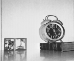
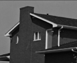
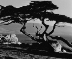
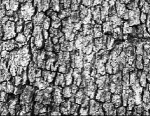
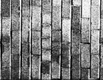
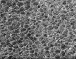
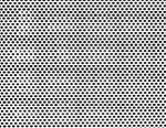
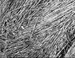
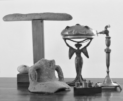
Figure 1: Set of test images. First and second rows are natural images: added value, boat, clock, house, tree, and test. The latter is not natural but it actually behaves as such in the denoising procedure. Third row are texture images: bark, bricks, bubbles, holes, and straw. All of them are of size 512×512512512512\times 512 but clock and test, which are 256×256256256256\times 256.

The comparison of the methods is done on two classes of intensity images: natural images and texture images, most of them obtained from the SIPI111Signal and Image Processing Institute, University of Southern California. data set, see Figure 1. We add to the original image, ucleansubscript𝑢cleanu_{\rm clean}, a Gaussian white noise to obtain the noisy image, unoisysubscript𝑢noisyu_{\rm noisy}, with fixed signal to noise ratio SNR=10SNR10\operatorname{SNR}=10, where

SNR=σ(uclean)σ(ucleanunoisy),SNR𝜎subscript𝑢clean𝜎subscript𝑢cleansubscript𝑢noisy\operatorname{SNR}=\frac{\sigma(u_{\rm clean})}{\sigma(u_{\rm clean}-u_{\rm noisy})},

being σ𝜎\sigma the standard deviation. After filtering unoisysubscript𝑢noisyu_{\rm noisy} with each method, we obtain a denoised image, udenoisedsubscript𝑢denoisedu_{\rm denoised}, that we compare to ucleansubscript𝑢cleanu_{\rm clean} using three quality measures [29]:

  • The pick signal to noise ratio (PSNR), given by

    PSNR(u1,u2)=20log10(255u1u22).PSNRsubscript𝑢1subscript𝑢220subscript10255subscriptnormsubscript𝑢1subscript𝑢22\displaystyle{\rm PSNR}(u_{1},u_{2})=20\log_{10}\Big{(}\frac{255}{\|u_{1}-u_{2}\|_{2}}\Big{)}.
  • The normalized cross correlation (NCC), given by

    NCC(u1,u2)=u1,u2u12u22[0,1].NCCsubscript𝑢1subscript𝑢2subscript𝑢1subscript𝑢2subscriptnormsubscript𝑢12subscriptnormsubscript𝑢2201\displaystyle{\rm NCC}(u_{1},u_{2})=\frac{\langle u_{1},u_{2}\rangle}{\|u_{1}\|_{2}\|u_{2}\|_{2}}\in[0,1].
  • The structural similarity (SSIM), given by

    SSIM(u1,u2)=(2μ1μ2+c1)(2σ1,2+c2)(μ12+μ22+c1)(σ12+σ22+c2)[0,1],SSIMsubscript𝑢1subscript𝑢22subscript𝜇1subscript𝜇2subscript𝑐12subscript𝜎12subscript𝑐2superscriptsubscript𝜇12superscriptsubscript𝜇22subscript𝑐1superscriptsubscript𝜎12superscriptsubscript𝜎22subscript𝑐201\displaystyle{\rm SSIM}(u_{1},u_{2})=\frac{(2\mu_{1}\mu_{2}+c_{1})(2\sigma_{1,2}+c_{2})}{(\mu_{1}^{2}+\mu_{2}^{2}+c_{1})(\sigma_{1}^{2}+\sigma_{2}^{2}+c_{2})}\in[0,1],

    where μi,σi,σi,jsubscript𝜇𝑖subscript𝜎𝑖subscript𝜎𝑖𝑗\mu_{i},~{}\sigma_{i},~{}\sigma_{i,j} stand for the mean, the standard deviation and the covariance of the corresponding images, and cisubscript𝑐𝑖c_{i} are some positive small constants included to avoid instability when the denominators are close to zero.

Since different methods have different sets of structural parameters which must be fixed for actual implementation, we have experimentally optimized them for each image in a reasonable range of values. The optimization has been performed with respect to the PSNR between the original and the denoised images.

3.1 Discretization

We use the well-posed QSS aproximation (19)-(20) of the cross-diffusion problem (12)-(14) to discretize in time. A similar approach is followed for the Perona-Malik equation (1). Then, for the cross-diffusion problem and for the gradient based Perona-Malik equation, that is, when gg(|u|)𝑔𝑔𝑢g\equiv g(|\nabla u|), we use the finite element method (FEM) to discretize in space, with linear-wise basis. For the Laplacian based Perona-Malik equation, the use of FEM would require to consider a basis of, at least, piece-wise quadratic polynomials to approximate the second order derivatives. Instead of incrementing the order of the FEM basis, we preferred to use a simpler scheme for this filter, based on the finite differences method.

We give the implementation details for the cross-diffusion system, being that of the Perona-Malik equation similar. Following [18], we fix the initial data as 𝐮0=(unoisy,0)subscript𝐮0subscript𝑢noisy0\mathbf{u}_{0}=(u_{\rm noisy},0) and consider the edge detector function as given by

g(𝐮)=g(u2),with g(s)=exp(s2/λcd2),formulae-sequence𝑔𝐮𝑔subscript𝑢2with 𝑔𝑠superscript𝑠2superscriptsubscript𝜆𝑐𝑑2g(\mathbf{u})=g(u_{2}),\quad\text{with }g(s)=\exp\big{(}-s^{2}/\lambda_{cd}^{2}\big{)},

with λcd>0subscript𝜆𝑐𝑑0\lambda_{cd}>0 optimized according to each method and image. The right hand side of (12) is taken as fi0subscript𝑓𝑖0f_{i}\equiv 0 (pure filtering case). Finally, like in [18], the diffusion coefficient matrix is taken as, for fixed θ[0,π/2)𝜃0𝜋2\theta\in[0,\pi/2),

A=(cosθsinθsinθcosθ),𝐴matrix𝜃𝜃𝜃𝜃A=\begin{pmatrix}\cos\theta&-\sin\theta\\ \sin\theta&\cos\theta\end{pmatrix},

with θ=π/30𝜃𝜋30\theta=\pi/30 in the experiments.

We used the open source software deal.II [3] to implement a time semi-implicit scheme with spatial linear-wise finite element discretization. For the time discretization, we take in the experiments a uniform partition of [0,T]0𝑇[0,T] of time step τ𝜏\tau. For the spatial discretization, we take the natural uniform partition of the rectangle [0,W]×[0,H]0𝑊0𝐻[0,W]\times[0,H], where W𝑊W and H𝐻H stand for the width and height (in pixels) of the given image, respectively.

Let, initially, t=t0=0𝑡subscript𝑡00t=t_{0}=0 and set ui0=ui0superscriptsubscript𝑢𝑖0subscript𝑢𝑖0u_{i}^{0}=u_{i0}. For n1𝑛1n\geq 1 the problem is: Find uinShsuperscriptsubscript𝑢𝑖𝑛superscript𝑆u_{i}^{n}\in S^{h} such that for i=1,2𝑖12i=1,2,

1τ(uinuin1,χ)h+(g(u2n)(ai1u1n+ai2u2n),χ)h=0,1𝜏superscriptsubscriptsuperscript𝑢𝑛𝑖subscriptsuperscript𝑢𝑛1𝑖𝜒superscript𝑔superscriptsubscript𝑢2𝑛subscript𝑎𝑖1superscriptsubscript𝑢1𝑛subscript𝑎𝑖2superscriptsubscript𝑢2𝑛𝜒0\begin{array}[]{l}\frac{1}{\tau}\big{(}u^{n}_{i}-u^{n-1}_{i},\chi)^{h}+\big{(}g(u_{2}^{n})(a_{i1}\nabla u_{1}^{n}+a_{i2}\nabla u_{2}^{n}),\nabla\chi\big{)}^{h}=0,\end{array} (21)

for every χSh𝜒superscript𝑆\chi\in S^{h}, the finite element space of piecewise 1subscript1\mathbb{Q}_{1}-elements. Here, (,)hsuperscript(\cdot,\cdot)^{h} stands for a discrete semi-inner product on 𝒞(Ω¯)𝒞¯Ω\mathcal{C}(\overline{\Omega}).

Since (21) is a nonlinear algebraic problem, we use a fixed point argument to approximate its solution, (u1n,u2n)superscriptsubscript𝑢1𝑛superscriptsubscript𝑢2𝑛(u_{1}^{n},u_{2}^{n}), at each time slice t=tn𝑡subscript𝑡𝑛t=t_{n}, from the previous approximation uin1superscriptsubscript𝑢𝑖𝑛1u_{i}^{n-1}. Let uin,0=uin1superscriptsubscript𝑢𝑖𝑛0superscriptsubscript𝑢𝑖𝑛1u_{i}^{n,0}=u_{i}^{n-1}. Then, for k1𝑘1k\geq 1 the linear problem to solve is: Find uin,ksuperscriptsubscript𝑢𝑖𝑛𝑘u_{i}^{n,k} such that for i=1,2𝑖12i=1,2, and for all χSh𝜒superscript𝑆\chi\in S^{h}

1τ(uin,kuin1,χ)h+(g(u2n,k1)(ai1u1n,k+ai2u2n,k),χ)h=0.1𝜏superscriptsubscriptsuperscript𝑢𝑛𝑘𝑖subscriptsuperscript𝑢𝑛1𝑖𝜒superscript𝑔superscriptsubscript𝑢2𝑛𝑘1subscript𝑎𝑖1superscriptsubscript𝑢1𝑛𝑘subscript𝑎𝑖2superscriptsubscript𝑢2𝑛𝑘𝜒0\begin{array}[]{l}\frac{1}{\tau}\big{(}u^{n,k}_{i}-u^{n-1}_{i},\chi)^{h}+\big{(}g(u_{2}^{n,k-1})(a_{i1}\nabla u_{1}^{n,k}+a_{i2}\nabla u_{2}^{n,k}),\nabla\chi\big{)}^{h}=0.\end{array}

We use the stopping criteria

maxi=1,2uin,kuin,k12<tol,subscript𝑖12subscriptnormsuperscriptsubscript𝑢𝑖𝑛𝑘superscriptsubscript𝑢𝑖𝑛𝑘12tol\max_{i=1,2}\|u_{i}^{n,k}-u_{i}^{n,k-1}\|_{2}<\text{tol}, (22)

for values of tol chosen empirically, and set uin=uin,ksuperscriptsubscript𝑢𝑖𝑛superscriptsubscript𝑢𝑖𝑛𝑘u_{i}^{n}=u_{i}^{n,k}. See Algorithm 1 for implementation details.

Turning to the neighborhood one-step filters, we used the simplest version of the Bilateral filter, also known as Yaroslavsky filter [30], given by

Yu(𝐱)=1C(𝐱)Bρ(𝐱)exp(|u(𝐱)u(𝐲)|2h2)u(𝐲)𝑑𝐲,Y𝑢𝐱1𝐶𝐱subscriptsubscript𝐵𝜌𝐱superscript𝑢𝐱𝑢𝐲2superscript2𝑢𝐲differential-d𝐲\displaystyle\operatorname{Y}u(\mathbf{x})=\frac{1}{C(\mathbf{x})}\int_{B_{\rho}(\mathbf{x})}\exp\Big{(}-\frac{|u(\mathbf{x})-u(\mathbf{y})|^{2}}{h^{2}}\Big{)}u(\mathbf{y})d\mathbf{y},

where Bρ(𝐱)subscript𝐵𝜌𝐱B_{\rho}(\mathbf{x}) is a box of diameter 4ρ4𝜌4\rho centered at 𝐱𝐱\mathbf{x}, and ρ,h𝜌\rho,~{}h are positive parameters. The term C(𝐱)𝐶𝐱C(\mathbf{x}) is the normalizing factor

C(𝐱)=Bρ(𝐱)exp(|u(𝐱)u(𝐲)|2h2)𝑑𝐲.𝐶𝐱subscriptsubscript𝐵𝜌𝐱superscript𝑢𝐱𝑢𝐲2superscript2differential-d𝐲\displaystyle C(\mathbf{x})=\int_{B_{\rho}(\mathbf{x})}\exp\Big{(}-\frac{|u(\mathbf{x})-u(\mathbf{y})|^{2}}{h^{2}}\Big{)}d\mathbf{y}.

For its implementation, we used the fast algorithm introduced in [24, 13, 14].

The Nonlocal Means filter is defined as

NLMu(𝐱)=1C(𝐱)Ωexp(Mσ(𝐱,𝐲)h2)u(𝐲)𝑑𝐲,NLM𝑢𝐱1𝐶𝐱subscriptΩsubscript𝑀𝜎𝐱𝐲superscript2𝑢𝐲differential-d𝐲\displaystyle\operatorname{NLM}u(\mathbf{x})=\frac{1}{C(\mathbf{x})}\int_{\Omega}\exp\Big{(}-\frac{M_{\sigma}(\mathbf{x},\mathbf{y})}{h^{2}}\Big{)}u(\mathbf{y})d\mathbf{y},

with h>00h>0, and the normalizing factor

C(𝐱)=Ωexp(Mσ(𝐱,𝐲)h2)𝑑𝐲.𝐶𝐱subscriptΩsubscript𝑀𝜎𝐱𝐲superscript2differential-d𝐲\displaystyle C(\mathbf{x})=\int_{\Omega}\exp\Big{(}-\frac{M_{\sigma}(\mathbf{x},\mathbf{y})}{h^{2}}\Big{)}d\mathbf{y}.

The nonlocal term, Mσsubscript𝑀𝜎M_{\sigma}, is given in convolution form by

Mσ(𝐱,𝐲)=2Gσ(𝐳)|u(𝐱+𝐳)u(𝐲+𝐳)|2𝑑𝐳,subscript𝑀𝜎𝐱𝐲subscriptsuperscript2subscript𝐺𝜎𝐳superscript𝑢𝐱𝐳𝑢𝐲𝐳2differential-d𝐳\displaystyle M_{\sigma}(\mathbf{x},\mathbf{y})=\int_{\mathbb{R}^{2}}G_{\sigma}(\mathbf{z})|u(\mathbf{x}+\mathbf{z})-u(\mathbf{y}+\mathbf{z})|^{2}d\mathbf{z},

where Gσsubscript𝐺𝜎G_{\sigma} is a Gaussian of standard deviation σ𝜎\sigma. In practice, the parameter hh is fixed in terms of σ𝜎\sigma, so this method has a single parameter to be optimized. For the discrete implementation, we used the patch-wise approach introduced by the authors [5].

Algorithm 1 FEM-Fixed point method for cross-diffusion problem (21)
1:Noisy image: unoisysubscript𝑢𝑛𝑜𝑖𝑠𝑦u_{noisy}; Final time: T𝑇T; Time step: τ𝜏\tau
2:Diffusion matrix: a𝑎a; Edge detector function: g𝑔g
3:Tolerance tol𝑡𝑜𝑙tol for the fixed point method; Max. number of fixed point iterations: maxFpIter
4:Spatial domain
5:Compute triangulation, function basis φ𝜑\varphi, and massMatrix
6:𝐮=(unoisy,0)𝐮subscript𝑢𝑛𝑜𝑖𝑠𝑦0\mathbf{u}=(u_{noisy},0), t=0𝑡0t=0
7:while t<T𝑡𝑇t<T do
8:     t+=τlimit-from𝑡𝜏t~{}+\!=~{}\tau
9:     𝐮old=𝐮subscript𝐮𝑜𝑙𝑑𝐮\mathbf{u}_{old}=\mathbf{u}, 𝐮fp=𝐮subscript𝐮𝑓𝑝𝐮\mathbf{u}_{fp}=\mathbf{u}, relDifference = \infty, fpIter=0
10:     while relDifference >> tol and fpIter << maxFpIter do
11:         fpIter +=+\!= 1
12:         𝐮fp,old=𝐮fpsubscript𝐮𝑓𝑝𝑜𝑙𝑑subscript𝐮𝑓𝑝\mathbf{u}_{fp,old}=\mathbf{u}_{fp}
13:         for All cells of the triangulation do
14:              cellMatrix = 0
15:              for All points in each cell do
16:                  edge=g(ufp,old,2)𝑒𝑑𝑔𝑒𝑔subscript𝑢𝑓𝑝𝑜𝑙𝑑2edge=g(u_{fp,old,2})
17:                  for φisubscript𝜑𝑖\varphi_{i}’s of cell basis do
18:                       for φjsubscript𝜑𝑗\varphi_{j}’s of cell basis do
19:                           cellMatrix(i,j)+=τedgea(i,j)φiφjarealimit-from𝑐𝑒𝑙𝑙𝑀𝑎𝑡𝑟𝑖𝑥𝑖𝑗𝜏𝑒𝑑𝑔𝑒𝑎𝑖𝑗subscript𝜑𝑖subscript𝜑𝑗𝑎𝑟𝑒𝑎cellMatrix(i,j)+\!=\tau*edge*a(i,j)*\nabla\varphi_{i}*\nabla\varphi_{j}*area                                                        
20:              Add cellMatrix contribution to systemMatrix          
21:         systemMatrix +=+\!= massMatrix
22:         if fpIter = 1 then
23:              RHS = systemMatrix*𝐮𝐮\mathbf{u}          
24:         Solve by LU method: systemMatrix*𝐮fpsubscript𝐮𝑓𝑝\mathbf{u}_{fp} = RHS
25:         Compute relative difference between 𝐮fpsubscript𝐮𝑓𝑝\mathbf{u}_{fp} and 𝐮fp,oldsubscript𝐮𝑓𝑝𝑜𝑙𝑑\mathbf{u}_{fp,old}      
26:      𝐮=𝐮fp𝐮subscript𝐮𝑓𝑝\mathbf{u}=\mathbf{u}_{fp}
27: 𝐮𝐮\mathbf{u}

3.2 Experiment data and results

Initial CD PM-L PM-G BF NLM
Parameters T𝑇T, λcdsubscript𝜆𝑐𝑑\lambda_{cd} T𝑇T, λpmsubscript𝜆𝑝𝑚\lambda_{pm} T𝑇T, λpmsubscript𝜆𝑝𝑚\lambda_{pm} hh, ρ𝜌\rho σ𝜎\sigma
added value
Opt. Par. (0.2, 0.15) (0.8, 10) (0.3, 20) (64, 4) 8
PSNR 31.8618 35.5620 34.0086 36.7013 36.2672 38.4068
NCC 0.9994 0.99975 0.99963 0.9998 0.99978 0.99987
SSIM 0.99503 0.99788 0.99695 0.99838 0.99819 0.99891
boat
Opt. Par. (0.1, 0.1) (0.3, 10) (0.1, 20) (12, 3) 5
PSNR 34.7000 36.2916 35.4629 36.4356 36.0391 36.9337
NCC 0.99942 0.9996 0.99952 0.99962 0.99957 0.99966
SSIM 0.99502 0.99653 0.99579 0.99666 0.9963 0.99702
clock
Opt. Par. (0.14, 0.15) (0.5, 10) (0.3, 20) (33, 4) 7
PSNR 32.9488 35.5378 34.187 37.0526 36.8077 38.4792
NCC 0.99957 0.99976 0.99968 0.99983 0.99982 0.99988
SSIM 0.99505 0.99726 0.99625 0.99809 0.99796 0.99863
house
Opt. Par. (0.13 , 0.15) (0.5, 10) (0.2, 20) (20, 3) 5
PSNR 34.4251 37.0206 35.7168 37.8745 37.7222 39.2158
NCC 0.99859 0.99924 0.99891 0.99937 0.99934 0.99954
SSIM 0.99504 0.99726 0.99608 0.99777 0.99769 0.99838
test
Opt. Par. (0.12, 0.1) (0.3, 10) (0.3, 25) (17, 64) 14
PSNR 28.8457 30.1614 29.1625 30.8796 32.5611 33.0273
NCC 0.99874 0.99916 0.9973 0.99928 0.99947 0.99964
SSIM 0.99711 0.99786 0.99408 0.9982 0.99881 0.9989
tree
Opt. Par. (0.12, 0.15) (0.4, 10) (0.25, 20) (35, 4) 8
PSNR 31.7344 33.7960 32.5588 34.7020 34.1934 35.2368
NCC 0.99795 0.99874 0.99617 0.99897 0.99884 0.9991
SSIM 0.99517 0.99697 0.99092 0.99756 0.99727 0.99785
Table 1: Optimal parameters and quality results for the set of natural images.
Measure Initial CD PM-L PM-G BF NLM
Parameters T𝑇T, λcdsubscript𝜆𝑐𝑑\lambda_{cd} T𝑇T, λpmsubscript𝜆𝑝𝑚\lambda_{pm} T𝑇T, λpmsubscript𝜆𝑝𝑚\lambda_{pm} hh, ρ𝜌\rho σ𝜎\sigma
bark
Opt. Par. (0.02, 0.3) (0.05, 50) (0.03, 70) (12, 6) 8
PSNR 30.8550 31.3764 30.9596 31.3815 30.9778 30.8820
NCC 0.99877 0.99892 0.99873 0.99892 0.99881 0.99878
SSIM 0.99517 0.99566 0.99492 0.99568 0.99528 0.9952
bricks
Opt. Par. (0.01, 0.25) (0.05, 50) (0.04, 50) (13, 5) 4
PSNR 30.8471 31.1076 30.975 31.1590 31.1448 30.9597
NCC 0.99878 0.99886 0.99881 0.99887 0.99886 0.99881
SSIM 0.99517 0.9954 0.99522 0.99547 0.99547 0.9953
bubbles
Opt. Par. (0.03, 0.1) (0.05, 30) (0.04, 40) (7, 3) 2
PSNR 36.1726 36.8475 36.3222 37.0446 36.3846 36.2160
NCC 0.99944 0.99953 0.99946 0.99955 0.99946 0.99945
SSIM 0.99502 0.99569 0.99515 0.9959 0.99518 0.99507
holes
Opt. Par. (0.03, 0.3) (0.05, 20) (0.15, 30) (14, 7) 14
PSNR 29.2774 29.9741 29.2695 29.9926 30.1212 30.1021
NCC 0.999 0.9992 0.99892 0.99916 0.99914 0.9992
SSIM 0.99617 0.99672 0.99584 0.99677 0.99681 0.99686
straw
Opt. Par. (0.01, 0.3) (0.01, 50) (0.02, 70) (12, 5) 14
PSNR 30.8735 31.1492 30.8961 31.1175 30.9911 30.8918
NCC 0.99878 0.99886 0.99875 0.99885 0.99881 0.99878
SSIM 0.99518 0.99542 0.99506 0.99541 0.99528 0.9952
Table 2: Optimal parameters and quality results for the set of texture images.

For the cross-diffusion and the Perona-Malik equations, the time step is fixed as τ=0.01𝜏0.01\tau=0.01, and the tolerance for the fixed point iteration inside each time loop, see (22), is taken as tol=103tolsuperscript103{\rm tol}=10^{-3}.

In Table 1 we show the optimal parameters found for each method, in the sense of PSNR maximization, and the resulting quality measures for each image in the set of natural images. For most of these images, the Laplacian based Perona-Malik equation gives the poorest results. The cross-diffusion, the gradient based Perona-Malik equation and the Bilateral (Yaroslavsky) filters give, in general, similar results. The Nonlocal Means filter outperforms the other methods for all the images.

In Table 2 we present the same information for the set of texture images. In this case the results are not conclusive. The relative performance among methods is closer than in the case of natural images and, in fact, the cross-diffusion and the gradient based Perona-Malik equations give the best results for most of the images. However, the denoising capacity of all of them is very limited and the denoising effect is hard to visualize.

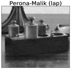
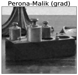
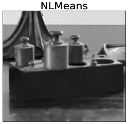
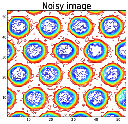
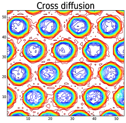
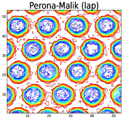
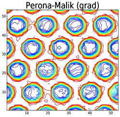
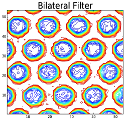
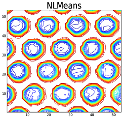
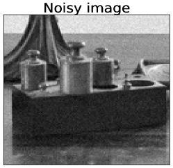
In Figure 2 we show a detail of the image added value showing the performance of all the methods for a natural image. In Figure 3 we show the contours plots for a detail of the texture image holes.
Refer to caption
Refer to caption
Refer to caption
Refer to caption
Refer to caption
Refer to caption
Figure 2: Detail of the natural image added value showing the performance of each method.
Refer to caption
Refer to caption
Refer to caption
Refer to caption
Refer to caption
Refer to caption
Figure 3: Contours plots for a detail of the texture image holes.

4 Proofs

Proof of Theorem 1. We start considering the following problem: Find 𝐮:Ω2:𝐮Ωsuperscript2\mathbf{u}:\Omega\to\mathbb{R}^{2} such that, for i=1,2𝑖12i=1,2, and ij𝑖𝑗i\neq j,

γiuidet(A)ajjdiv(g(𝐮)ui)=GiαijGj+αijγjujsubscript𝛾𝑖subscript𝑢𝑖𝐴subscript𝑎𝑗𝑗div𝑔𝐮subscript𝑢𝑖subscript𝐺𝑖subscript𝛼𝑖𝑗subscript𝐺𝑗subscript𝛼𝑖𝑗subscript𝛾𝑗subscript𝑢𝑗\displaystyle\gamma_{i}u_{i}-\frac{\det(A)}{a_{jj}}\operatorname{div}\big{(}g(\mathbf{u})\nabla u_{i}\big{)}=G_{i}-\alpha_{ij}G_{j}+\alpha_{ij}\gamma_{j}u_{j} in Ω,in Ω\displaystyle\quad\text{in }\Omega, (23)
g(𝐮)uiν=0𝑔𝐮subscript𝑢𝑖𝜈0\displaystyle g(\mathbf{u})\nabla u_{i}\cdot\nu=0 on Ω.on Ω\displaystyle\quad\text{on }\partial\Omega. (24)

with αij=aij/ajjsubscript𝛼𝑖𝑗subscript𝑎𝑖𝑗subscript𝑎𝑗𝑗\alpha_{ij}=a_{ij}/a_{jj}. Notice that, due to assumption (H)2,

det(A)>0,aii>0,and|αij|<1.formulae-sequence𝐴0formulae-sequencesubscript𝑎𝑖𝑖0andsubscript𝛼𝑖𝑗1\displaystyle\det(A)>0,\quad a_{ii}>0,\quad\text{and}\quad|\alpha_{ij}|<1.

Step 1: Linearizing. Let 𝐮~L2(Ω)2~𝐮superscript𝐿2superscriptΩ2\tilde{\mathbf{u}}\in L^{2}(\Omega)^{2} be given and consider the function gk(s1,s2)=g(Tk(s1),Tk(s2))subscript𝑔𝑘subscript𝑠1subscript𝑠2𝑔subscript𝑇𝑘subscript𝑠1subscript𝑇𝑘subscript𝑠2g_{k}(s_{1},s_{2})=g(T_{k}(s_{1}),T_{k}(s_{2})), with the truncation function Tk::subscript𝑇𝑘T_{k}:\mathbb{R}\to\mathbb{R} given by

Tk(s)={kif sk,sif ksk,kif sk.subscript𝑇𝑘𝑠cases𝑘if 𝑠𝑘𝑠if 𝑘𝑠𝑘𝑘if 𝑠𝑘\displaystyle T_{k}(s)=\left\{\begin{array}[]{ll}-k&\text{if }s\leq-k,\\ s&\text{if }-k\leq s\leq k,\\ k&\text{if }s\geq k.\end{array}\right.

Let σ[0,1]𝜎01\sigma\in[0,1]. We set the following linear problem: Find 𝐮H1(Ω)2𝐮superscript𝐻1superscriptΩ2\mathbf{u}\in H^{1}(\Omega)^{2} such that for i=1,2𝑖12i=1,2, and ij𝑖𝑗i\neq j,

γiuidet(A)ajjdiv(gk(𝐮~)ui)=σ(GiαijGj)+αijγjujsubscript𝛾𝑖subscript𝑢𝑖𝐴subscript𝑎𝑗𝑗divsubscript𝑔𝑘~𝐮subscript𝑢𝑖𝜎subscript𝐺𝑖subscript𝛼𝑖𝑗subscript𝐺𝑗subscript𝛼𝑖𝑗subscript𝛾𝑗subscript𝑢𝑗\displaystyle\gamma_{i}u_{i}-\frac{\det(A)}{a_{jj}}\operatorname{div}\big{(}g_{k}(\tilde{\mathbf{u}})\nabla u_{i}\big{)}=\sigma(G_{i}-\alpha_{ij}G_{j})+\alpha_{ij}\gamma_{j}u_{j} in Ω,in Ω\displaystyle\quad\text{in }\Omega, (25)
gk(𝐮~)uiν=0subscript𝑔𝑘~𝐮subscript𝑢𝑖𝜈0\displaystyle g_{k}(\tilde{\mathbf{u}})\nabla u_{i}\cdot\nu=0 on Ω.on Ω\displaystyle\quad\text{on }\partial\Omega. (26)

Since, gk(2)g(K)subscript𝑔𝑘superscript2𝑔𝐾g_{k}(\mathbb{R}^{2})\subset g(K), with K=[k,k]×[k,k]𝐾𝑘𝑘𝑘𝑘K=[-k,k]\times[-k,k], and by assumption (H)3, g(K)(0,)𝑔𝐾0g(K)\subset(0,\infty), that is, the problem is uniformly elliptic, we may apply [21][Chapter 6, Theorem 2.1], to deduce the existence of a unique weak solution 𝐮H1(Ω)2L(Ω)2𝐮superscript𝐻1superscriptΩ2superscript𝐿superscriptΩ2\mathbf{u}\in H^{1}(\Omega)^{2}\cap L^{\infty}(\Omega)^{2} of problem (25)-(26).

We now show that the L(Ω)superscript𝐿ΩL^{\infty}(\Omega) bound does not depend on 𝐮~~𝐮\tilde{\mathbf{u}} or k𝑘k. Let [s]+subscriptdelimited-[]𝑠[s]_{+} and [s]subscriptdelimited-[]𝑠[s]_{-} denote the positive and negative parts of s𝑠s, so that s=[s]+[s]𝑠subscriptdelimited-[]𝑠subscriptdelimited-[]𝑠s=[s]_{+}-[s]_{-}. Taking, for p1𝑝1p\geq 1, [ui]+pH1(Ω)superscriptsubscriptdelimited-[]subscript𝑢𝑖𝑝superscript𝐻1Ω[u_{i}]_{+}^{p}\in H^{1}(\Omega) as test function in the weak formulation of (25)-(26), and using Young’s inequlity, we deduce

γi[ui]+p+1σ(Gip+1+|αij|Gjp+1)+γj|αij|[uj]+p+1.subscript𝛾𝑖subscriptnormsubscriptdelimited-[]subscript𝑢𝑖𝑝1𝜎subscriptnormsubscript𝐺𝑖𝑝1subscript𝛼𝑖𝑗subscriptnormsubscript𝐺𝑗𝑝1subscript𝛾𝑗subscript𝛼𝑖𝑗subscriptnormsubscriptdelimited-[]subscript𝑢𝑗𝑝1\displaystyle\gamma_{i}\|[u_{i}]_{+}\|_{p+1}\leq\sigma\big{(}\|G_{i}\|_{p+1}+|\alpha_{ij}|\|G_{j}\|_{p+1}\big{)}+\gamma_{j}|\alpha_{ij}|\|[u_{j}]_{+}\|_{p+1}.

Summing for i,j=1,2formulae-sequence𝑖𝑗12i,j=1,2, with ij𝑖𝑗i\neq j, we obtain

γ1(1|α21|)subscript𝛾11subscript𝛼21\displaystyle\gamma_{1}(1-|\alpha_{21}|) [u1]+p+1+γ2(1|α12|)[u2]+p+1subscriptnormsubscriptdelimited-[]subscript𝑢1𝑝1subscript𝛾21subscript𝛼12subscriptnormsubscriptdelimited-[]subscript𝑢2𝑝1\displaystyle\|[u_{1}]_{+}\|_{p+1}+\gamma_{2}(1-|\alpha_{12}|)\|[u_{2}]_{+}\|_{p+1}
σ(1+|α21|)G1p+1+σ(1+|α12|)G2p+1absent𝜎1subscript𝛼21subscriptnormsubscript𝐺1𝑝1𝜎1subscript𝛼12subscriptnormsubscript𝐺2𝑝1\displaystyle\leq\sigma\big{(}1+|\alpha_{21}|\big{)}\|G_{1}\|_{p+1}+\sigma\big{(}1+|\alpha_{12}|\big{)}\|G_{2}\|_{p+1}

A similar estimate holds for [ui]p+1superscriptsubscriptdelimited-[]subscript𝑢𝑖𝑝1[u_{i}]_{-}^{p+1}, so we obtain, taking the limit p𝑝p\to\infty,

γ1(1|α21|)u1+limit-fromsubscript𝛾11subscript𝛼21subscriptnormsubscript𝑢1\displaystyle\gamma_{1}(1-|\alpha_{21}|)\|u_{1}\|_{\infty}+ γ2(1|α12|)u2subscript𝛾21subscript𝛼12subscriptnormsubscript𝑢2\displaystyle\gamma_{2}(1-|\alpha_{12}|)\|u_{2}\|_{\infty}
σ(1+|α21|)G1+σ(1+|α12|)G2.absent𝜎1subscript𝛼21subscriptnormsubscript𝐺1𝜎1subscript𝛼12subscriptnormsubscript𝐺2\displaystyle\leq\sigma\big{(}1+|\alpha_{21}|\big{)}\|G_{1}\|_{\infty}+\sigma\big{(}1+|\alpha_{12}|\big{)}\|G_{2}\|_{\infty}. (27)

Step 2: Fixed point. Consider the operator P:L2(Ω)2×[0,1]L2(Ω)2:𝑃superscript𝐿2superscriptΩ201superscript𝐿2superscriptΩ2P:L^{2}(\Omega)^{2}\times[0,1]\to L^{2}(\Omega)^{2} given by P(𝐮~,σ)=𝐮𝑃~𝐮𝜎𝐮P(\tilde{\mathbf{u}},\sigma)=\mathbf{u}, being 𝐮𝐮\mathbf{u} the solution of the linear problem (25)-(26) corresponding to (𝐮~,σ)~𝐮𝜎(\tilde{\mathbf{u}},\sigma). We check that P𝑃P satisfies the conditions of the Leray-Schauder’s Fixed Point theorem, that is

  1. 1.

    P𝑃P is continuous and compact.

  2. 2.

    P(𝐯,0)=0𝑃𝐯00P(\mathbf{v},0)=0 for all 𝐯L2(Ω)2𝐯superscript𝐿2superscriptΩ2\mathbf{v}\in L^{2}(\Omega)^{2}.

  3. 3.

    The fixed points of P𝑃P are uniformly bounded in L2(Ω)2superscript𝐿2superscriptΩ2L^{2}(\Omega)^{2}.

1. Let 𝐯nL2(Ω)subscript𝐯𝑛superscript𝐿2Ω\mathbf{v}_{n}\in L^{2}(\Omega) be a sequence strongly convergent to 𝐯L2(Ω)𝐯superscript𝐿2Ω\mathbf{v}\in L^{2}(\Omega), and σnσsubscript𝜎𝑛𝜎\sigma_{n}\to\sigma. Define 𝐮n=P(𝐯n,σn)subscript𝐮𝑛𝑃subscript𝐯𝑛subscript𝜎𝑛\mathbf{u}_{n}=P(\mathbf{v}_{n},\sigma_{n}). Using ui,nH1(Ω)subscript𝑢𝑖𝑛superscript𝐻1Ωu_{i,n}\in H^{1}(\Omega) as a test function in the weak formulation of (25)-(26) leads to

γiΩ|ui,n|2+det(A)ajjmin(g(K))Ω|ui,n|2subscript𝛾𝑖subscriptΩsuperscriptsubscript𝑢𝑖𝑛2𝐴subscript𝑎𝑗𝑗𝑔𝐾subscriptΩsuperscriptsubscript𝑢𝑖𝑛2absent\displaystyle\gamma_{i}\int_{\Omega}|u_{i,n}|^{2}+\frac{\det(A)}{a_{jj}}\min(g(K))\int_{\Omega}|\nabla u_{i,n}|^{2}\leq σnΩ(|Gi|+|αij||Gj|)|ui,n|subscript𝜎𝑛subscriptΩsubscript𝐺𝑖subscript𝛼𝑖𝑗subscript𝐺𝑗subscript𝑢𝑖𝑛\displaystyle\sigma_{n}\int_{\Omega}(|G_{i}|+|\alpha_{ij}||G_{j}|)|u_{i,n}|
+|αij|Ω|ui,n||uj,n|.subscript𝛼𝑖𝑗subscriptΩsubscript𝑢𝑖𝑛subscript𝑢𝑗𝑛\displaystyle+|\alpha_{ij}|\int_{\Omega}|u_{i,n}||u_{j,n}|. (28)

We first use Hölder’s inequality to deduce, after summing for i,j=1,2formulae-sequence𝑖𝑗12i,j=1,2, with ij𝑖𝑗i\neq j

γ1(1|α21|)subscript𝛾11subscript𝛼21\displaystyle\gamma_{1}(1-|\alpha_{21}|) u122+γ2(1|α12|)u222superscriptsubscriptnormsubscript𝑢122subscript𝛾21subscript𝛼12superscriptsubscriptnormsubscript𝑢222\displaystyle\|u_{1}\|_{2}^{2}+\gamma_{2}(1-|\alpha_{12}|)\|u_{2}\|_{2}^{2}
σn(1+|α21|)G122+σn(1+|α12|)G222,absentsubscript𝜎𝑛1subscript𝛼21superscriptsubscriptnormsubscript𝐺122subscript𝜎𝑛1subscript𝛼12superscriptsubscriptnormsubscript𝐺222\displaystyle\leq\sigma_{n}\big{(}1+|\alpha_{21}|\big{)}\|G_{1}\|_{2}^{2}+\sigma_{n}\big{(}1+|\alpha_{12}|\big{)}\|G_{2}\|_{2}^{2},

and then, from (28), we also deduce that ui,n2subscriptnormsubscript𝑢𝑖𝑛2\|\nabla u_{i,n}\|_{2} is uniformly bounded. Therefore, there exists a subsequence of 𝐮nsubscript𝐮𝑛\mathbf{u}_{n} (not relabeled), and a function 𝐮H1(Ω)2𝐮superscript𝐻1superscriptΩ2\mathbf{u}\in H^{1}(\Omega)^{2}, such that

ui,nuisubscript𝑢𝑖𝑛subscript𝑢𝑖\displaystyle\nabla u_{i,n}\rightharpoonup\nabla u_{i} weakly in L2(Ω),weakly in superscript𝐿2Ω\displaystyle\text{weakly in }L^{2}(\Omega),
ui,nuisubscript𝑢𝑖𝑛subscript𝑢𝑖\displaystyle u_{i,n}\to u_{i} strongly in L2(Ω).strongly in superscript𝐿2Ω\displaystyle\text{strongly in }L^{2}(\Omega).

Since, by assumption, vi,nvisubscript𝑣𝑖𝑛subscript𝑣𝑖v_{i,n}\to v_{i} in L2(Ω)superscript𝐿2ΩL^{2}(\Omega) (and a.e. in ΩΩ\Omega, for a subsequence), and gk(vi,n)subscriptnormsubscript𝑔𝑘subscript𝑣𝑖𝑛\|g_{k}(v_{i,n})\|_{\infty} is uniformly bounded with respect to n𝑛n, we deduce by the dominated convergence theorem that gk(vi,n)gk(vi)subscript𝑔𝑘subscript𝑣𝑖𝑛subscript𝑔𝑘subscript𝑣𝑖g_{k}(v_{i,n})\to g_{k}(v_{i}) in Lq(Ω)superscript𝐿𝑞ΩL^{q}(\Omega), for all q<𝑞q<\infty. Therefore,

gk(𝐯n)ui,ngk(𝐯)uiweakly in Lγ(Ω)subscript𝑔𝑘subscript𝐯𝑛subscript𝑢𝑖𝑛subscript𝑔𝑘𝐯subscript𝑢𝑖weakly in superscript𝐿𝛾Ω\displaystyle g_{k}(\mathbf{v}_{n})\nabla u_{i,n}\rightharpoonup g_{k}(\mathbf{v})\nabla u_{i}\quad\text{weakly in }L^{\gamma}(\Omega)

for any γ<2𝛾2\gamma<2. But since the sequence gk(𝐯n)ui,nsubscript𝑔𝑘subscript𝐯𝑛subscript𝑢𝑖𝑛g_{k}(\mathbf{v}_{n})\nabla u_{i,n} is bounded in L2(Ω)superscript𝐿2ΩL^{2}(\Omega), we deduce that, in fact,

gk(𝐯n)ui,ngk(𝐯)uiweakly in L2(Ω).subscript𝑔𝑘subscript𝐯𝑛subscript𝑢𝑖𝑛subscript𝑔𝑘𝐯subscript𝑢𝑖weakly in superscript𝐿2Ω\displaystyle g_{k}(\mathbf{v}_{n})\nabla u_{i,n}\rightharpoonup g_{k}(\mathbf{v})\nabla u_{i}\quad\text{weakly in }L^{2}(\Omega).

The other terms in the weak formulation of (25)-(26) (with the replacements 𝐮~=𝐯n~𝐮subscript𝐯𝑛\tilde{\mathbf{u}}=\mathbf{v}_{n}, 𝐮=𝐮n𝐮subscript𝐮𝑛\mathbf{u}=\mathbf{u}_{n}, and σ=σn𝜎subscript𝜎𝑛\sigma=\sigma_{n}) pass clearly to their corresponding limits. Finally, the uniqueness of solutions of problem (25)-(26) implies that the whole sequence 𝐮nsubscript𝐮𝑛\mathbf{u}_{n} converges to 𝐮𝐮\mathbf{u}. So the continuity follows. The compactness is directly deduced from the compact embedding H1(Ω)L2(Ω)superscript𝐻1Ωsuperscript𝐿2ΩH^{1}(\Omega)\subset L^{2}(\Omega).

2. If 𝐮=P(𝐯,0)𝐮𝑃𝐯0\mathbf{u}=P(\mathbf{v},0) then, in particular, 𝐮𝐮\mathbf{u} satisfies estimate (27) with σ=0𝜎0\sigma=0. Thus, 𝐮=0𝐮0\mathbf{u}=0 a.e. in ΩΩ\Omega.

3. If 𝐮=S(𝐮,σ)𝐮𝑆𝐮𝜎\mathbf{u}=S(\mathbf{u},\sigma), we again use that 𝐮𝐮\mathbf{u} satisfies (27) with σ[0,1]𝜎01\sigma\in[0,1], to get the uniform bound of 𝐮𝐮\mathbf{u} in L2(Ω)superscript𝐿2ΩL^{2}(\Omega).

Thus, the Leray-Schauder’s fixed point theorem ensures the existence of a fixed point, 𝐮𝐮\mathbf{u}, of P(𝐮,1)𝑃𝐮1P(\mathbf{u},1), which is a solution of (23)-(24) with g𝑔g replaced by gksubscript𝑔𝑘g_{k}. But since this fixed point satisfies the L(Ω)superscript𝐿ΩL^{\infty}(\Omega) bound (27) (with σ=1𝜎1\sigma=1), we deduce that for k𝑘k large enough gk(𝐮)=g(𝐮)subscript𝑔𝑘𝐮𝑔𝐮g_{k}(\mathbf{u})=g(\mathbf{u}), and thus 𝐮𝐮\mathbf{u} is a solution of (23)-(24).

Step 3: Solution of the original problem (17)-(18). The weak solution, 𝐮𝐮\mathbf{u}, of problem (23)-(24) satisfies, for all φH1(Ω)𝜑superscript𝐻1Ω\varphi\in H^{1}(\Omega),

γ1Ωu1φ+det(A)a22Ωg(𝐮)u1φ=ΩG1φα12ΩG2φ+α12γ2Ωu2φ,subscript𝛾1subscriptΩsubscript𝑢1𝜑𝐴subscript𝑎22subscriptΩ𝑔𝐮subscript𝑢1𝜑subscriptΩsubscript𝐺1𝜑subscript𝛼12subscriptΩsubscript𝐺2𝜑subscript𝛼12subscript𝛾2subscriptΩsubscript𝑢2𝜑\displaystyle\gamma_{1}\int_{\Omega}u_{1}\varphi+\frac{\det(A)}{a_{22}}\int_{\Omega}g(\mathbf{u})\nabla u_{1}\cdot\nabla\varphi=\int_{\Omega}G_{1}\varphi-\alpha_{12}\int_{\Omega}G_{2}\varphi+\alpha_{12}\gamma_{2}\int_{\Omega}u_{2}\varphi,
γ2Ωu2φ+det(A)a11Ωg(𝐮)u2φ=ΩG2φα21ΩG1φ+α21γ1Ωu1φ.subscript𝛾2subscriptΩsubscript𝑢2𝜑𝐴subscript𝑎11subscriptΩ𝑔𝐮subscript𝑢2𝜑subscriptΩsubscript𝐺2𝜑subscript𝛼21subscriptΩsubscript𝐺1𝜑subscript𝛼21subscript𝛾1subscriptΩsubscript𝑢1𝜑\displaystyle\gamma_{2}\int_{\Omega}u_{2}\varphi+\frac{\det(A)}{a_{11}}\int_{\Omega}g(\mathbf{u})\nabla u_{2}\cdot\nabla\varphi=\int_{\Omega}G_{2}\varphi-\alpha_{21}\int_{\Omega}G_{1}\varphi+\alpha_{21}\gamma_{1}\int_{\Omega}u_{1}\varphi.

Multiplying the first equation by a11a22/det(A)subscript𝑎11subscript𝑎22𝐴a_{11}a_{22}/\det(A), the second by a12a11/det(A)subscript𝑎12subscript𝑎11𝐴a_{12}a_{11}/\det(A) and adding the results leads to

γ1Ωu1φ+Ωg(𝐮)(a11u1+a12u2)φ=ΩG1φ.subscript𝛾1subscriptΩsubscript𝑢1𝜑subscriptΩ𝑔𝐮subscript𝑎11subscript𝑢1subscript𝑎12subscript𝑢2𝜑subscriptΩsubscript𝐺1𝜑\displaystyle\gamma_{1}\int_{\Omega}u_{1}\varphi+\int_{\Omega}g(\mathbf{u})(a_{11}\nabla u_{1}+a_{12}\nabla u_{2})\cdot\nabla\varphi=\int_{\Omega}G_{1}\varphi.

A similar combination, also gives

γ2Ωu2φ+Ωg(𝐮)(a21u1+a22u2)φ=ΩG2φ,subscript𝛾2subscriptΩsubscript𝑢2𝜑subscriptΩ𝑔𝐮subscript𝑎21subscript𝑢1subscript𝑎22subscript𝑢2𝜑subscriptΩsubscript𝐺2𝜑\displaystyle\gamma_{2}\int_{\Omega}u_{2}\varphi+\int_{\Omega}g(\mathbf{u})(a_{21}\nabla u_{1}+a_{22}\nabla u_{2})\cdot\nabla\varphi=\int_{\Omega}G_{2}\varphi,

so 𝐮𝐮\mathbf{u} is a weak solution of (17)-(18). \Box


Proof of Corollary 1. The proof follows easily from Theorem 1 by taking γi=βi+1/τ>0subscript𝛾𝑖subscript𝛽𝑖1𝜏0\gamma_{i}=\beta_{i}+1/\tau>0 and, recursively, Gi=βi0ui0+uin/τL(Ω)subscript𝐺𝑖subscript𝛽𝑖0subscript𝑢𝑖0superscriptsubscript𝑢𝑖𝑛𝜏superscript𝐿ΩG_{i}=\beta_{i0}u_{i0}+u_{i}^{n}/\tau\in L^{\infty}(\Omega). \Box

Remark 1.

The Lsuperscript𝐿L^{\infty} bound (27) of the steady state problem translates, in the case of the QSS approximation, to

u1n+1+u2n+1C1(u1n+u2n)+C2(u10+u20),subscriptnormsuperscriptsubscript𝑢1𝑛1subscriptnormsuperscriptsubscript𝑢2𝑛1subscript𝐶1subscriptnormsuperscriptsubscript𝑢1𝑛subscriptnormsuperscriptsubscript𝑢2𝑛subscript𝐶2subscriptnormsubscript𝑢10subscriptnormsubscript𝑢20\displaystyle\|u_{1}^{n+1}\|_{\infty}+\|u_{2}^{n+1}\|_{\infty}\leq C_{1}\big{(}\|u_{1}^{n}\|_{\infty}+\|u_{2}^{n}\|_{\infty}\big{)}+C_{2}\big{(}\|u_{10}\|_{\infty}+\|u_{20}\|_{\infty}\big{)},

with C1>1subscript𝐶11C_{1}>1 unless α12=α21=0subscript𝛼12subscript𝛼210\alpha_{12}=\alpha_{21}=0, that is, a12=a21=0subscript𝑎12subscript𝑎210a_{12}=a_{21}=0. Thus, this bound is not useful for passing to the limit τ0𝜏0\tau\to 0, and thus to prove the existence of the evolution problem, except when A𝐴A is diagonal.


Proof of Corollary 2.

Case 1: a12=a21=0subscript𝑎12subscript𝑎210a_{12}=a_{21}=0 (diagonal case). Consider the time discretization (19)-(20), for which the existence of a solution 𝐮n+1superscript𝐮𝑛1\mathbf{u}^{n+1} is guaranteed by Corollary 1. In this case, a finer Lsuperscript𝐿L^{\infty} estimate of each time slice may be obtained. Indeed, the Lp+1superscript𝐿𝑝1L^{p+1} estimate (27) of Step 1 of the proof of Corollary 1 reduces to

(1+τβi)uin+1p+1uinp+1+τβiu10p+1,1𝜏subscript𝛽𝑖subscriptnormsuperscriptsubscript𝑢𝑖𝑛1𝑝1subscriptnormsuperscriptsubscript𝑢𝑖𝑛𝑝1𝜏subscript𝛽𝑖subscriptnormsubscript𝑢10𝑝1\displaystyle(1+\tau\beta_{i})\|u_{i}^{n+1}\|_{p+1}\leq\|u_{i}^{n}\|_{p+1}+\tau\beta_{i}\|u_{10}\|_{p+1},

and thus we get

uin+111+τβiuin+τβi1+τβiui0.subscriptnormsuperscriptsubscript𝑢𝑖𝑛111𝜏subscript𝛽𝑖subscriptnormsuperscriptsubscript𝑢𝑖𝑛𝜏subscript𝛽𝑖1𝜏subscript𝛽𝑖subscriptnormsubscript𝑢𝑖0\displaystyle\|u_{i}^{n+1}\|_{\infty}\leq\frac{1}{1+\tau\beta_{i}}\|u_{i}^{n}\|_{\infty}+\frac{\tau\beta_{i}}{1+\tau\beta_{i}}\|u_{i0}\|_{\infty}.

Solving this differences inequality, we find the required uniform Lsuperscript𝐿L^{\infty} estimate for proving the convergence of time interpolators. Indeed, observe that this uniform estimate also implies a uniform estimate for uin+12subscriptnormsuperscriptsubscript𝑢𝑖𝑛12\|\nabla u_{i}^{n+1}\|_{2}, since by assumption g(𝐮n+1)𝑔superscript𝐮𝑛1g(\mathbf{u}^{n+1}) remains bounded away from zero for all n𝑛n\in\mathbb{N}.

Time interpolators and passing to the limit τ0𝜏0\tau\to 0. This step is somehow standard, so we give an sketch. We define, for (t,x)(tn,tn+1]×Ω𝑡𝑥subscript𝑡𝑛subscript𝑡𝑛1Ω(t,x)\in(t_{n},t_{n+1}]\times\Omega, the piecewise constant and piecewise linear interpolators

ui(τ)(t,x)=uin+1(x),u~i(τ)(t,x)=uin(x)+ttnτ(uin+1(x)uin(x)).formulae-sequencesuperscriptsubscript𝑢𝑖𝜏𝑡𝑥superscriptsubscript𝑢𝑖𝑛1𝑥superscriptsubscript~𝑢𝑖𝜏𝑡𝑥superscriptsubscript𝑢𝑖𝑛𝑥𝑡subscript𝑡𝑛𝜏superscriptsubscript𝑢𝑖𝑛1𝑥superscriptsubscript𝑢𝑖𝑛𝑥\displaystyle u_{i}^{(\tau)}(t,x)=u_{i}^{n+1}(x),\quad\tilde{u}_{i}^{(\tau)}(t,x)=u_{i}^{n}(x)+\frac{t-t_{n}}{\tau}(u_{i}^{n+1}(x)-u_{i}^{n}(x)).

Using the uniform estimates of uin+1subscriptnormsuperscriptsubscript𝑢𝑖𝑛1\|u_{i}^{n+1}\|_{\infty} and uin+12subscriptnormsuperscriptsubscript𝑢𝑖𝑛12\|\nabla u_{i}^{n+1}\|_{2}, we deduce the corresponding uniform estimates for ui(τ)L(QT)subscriptnormsuperscriptsubscript𝑢𝑖𝜏superscript𝐿subscript𝑄𝑇\|u_{i}^{(\tau)}\|_{L^{\infty}(Q_{T})}, u~i(τ)L(QT)subscriptnormsuperscriptsubscript~𝑢𝑖𝜏superscript𝐿subscript𝑄𝑇\|\tilde{u}_{i}^{(\tau)}\|_{L^{\infty}(Q_{T})}, and for

ui(τ)L2(QT),u~i(τ)L2(QT)tu~i(τ)L2(0,T;(H1(Ω))),subscriptnormsuperscriptsubscript𝑢𝑖𝜏superscript𝐿2subscript𝑄𝑇subscriptnormsuperscriptsubscript~𝑢𝑖𝜏superscript𝐿2subscript𝑄𝑇subscriptnormsubscript𝑡superscriptsubscript~𝑢𝑖𝜏superscript𝐿20𝑇superscriptsuperscript𝐻1Ω\|\nabla u_{i}^{(\tau)}\|_{L^{2}(Q_{T})},\quad\|\nabla\tilde{u}_{i}^{(\tau)}\|_{L^{2}(Q_{T})}\quad\|{\partial}_{t}\tilde{u}_{i}^{(\tau)}\|_{L^{2}(0,T;(H^{1}(\Omega))^{\prime})},

implying the existence of uiL2(0,T;H1(Ω))L(Ω)subscript𝑢𝑖superscript𝐿20𝑇superscript𝐻1Ωsuperscript𝐿Ωu_{i}\in L^{2}(0,T;H^{1}(\Omega))\cap L^{\infty}(\Omega) and

u~iL2(0,T;H1(Ω))H1(0,T;(H1(Ω)))L(Ω)subscript~𝑢𝑖superscript𝐿20𝑇superscript𝐻1Ωsuperscript𝐻10𝑇superscriptsuperscript𝐻1Ωsuperscript𝐿Ω\tilde{u}_{i}\in L^{2}(0,T;H^{1}(\Omega))\cap H^{1}(0,T;(H^{1}(\Omega))^{\prime})\cap L^{\infty}(\Omega)

such that, at least in a subsequence (not relabeled), as τ0𝜏0\tau\to 0,

ui(τ)uiweakly in L2(0,T;H1(Ω)),superscriptsubscript𝑢𝑖𝜏subscript𝑢𝑖weakly in superscript𝐿20𝑇superscript𝐻1Ω\displaystyle u_{i}^{(\tau)}\to u_{i}\quad\text{weakly in }L^{2}(0,T;H^{1}(\Omega)), (29)
ui(τ)uiweakly* in L(QT)),\displaystyle u_{i}^{(\tau)}\to u_{i}\quad\text{weakly* in }L^{\infty}(Q_{T})),
u~i(τ)u~iweakly in H1(0,T;(H1(Ω))),superscriptsubscript~𝑢𝑖𝜏subscript~𝑢𝑖weakly in superscript𝐻10𝑇superscriptsuperscript𝐻1Ω\displaystyle\tilde{u}_{i}^{(\tau)}\to\tilde{u}_{i}\quad\text{weakly in }H^{1}(0,T;(H^{1}(\Omega))^{\prime}), (30)
u~i(τ)u~iweakly in L2(0,T;H1(Ω)),superscriptsubscript~𝑢𝑖𝜏subscript~𝑢𝑖weakly in superscript𝐿20𝑇superscript𝐻1Ω\displaystyle\tilde{u}_{i}^{(\tau)}\to\tilde{u}_{i}\quad\text{weakly in }L^{2}(0,T;H^{1}(\Omega)), (31)
u~i(τ)u~iweakly* in L(QT)).\displaystyle\tilde{u}_{i}^{(\tau)}\to\tilde{u}_{i}\quad\text{weakly* in }L^{\infty}(Q_{T})).

In particular, by compactness

u~i(τ)u~istrongly in L2(QT).superscriptsubscript~𝑢𝑖𝜏subscript~𝑢𝑖strongly in superscript𝐿2subscript𝑄𝑇\tilde{u}_{i}^{(\tau)}\to\tilde{u}_{i}\quad\text{strongly in }L^{2}(Q_{T}).

Since u~i(τ)ui(τ)=τ(δt1)tu~i(τ)superscriptsubscript~𝑢𝑖𝜏superscriptsubscript𝑢𝑖𝜏𝜏𝛿𝑡1subscript𝑡superscriptsubscript~𝑢𝑖𝜏\tilde{u}_{i}^{(\tau)}-u_{i}^{(\tau)}=\tau(\delta t-1){\partial}_{t}\tilde{u}_{i}^{(\tau)}, with δt=t/τn[0,1]𝛿𝑡𝑡𝜏𝑛01\delta t=t/\tau-n\in[0,1], we also find

u~i(τ)ui(τ)L2(0,T;(H1(Ω)))0as τ0.formulae-sequencesubscriptnormsuperscriptsubscript~𝑢𝑖𝜏superscriptsubscript𝑢𝑖𝜏superscript𝐿20𝑇superscriptsuperscript𝐻1Ω0as 𝜏0\|\tilde{u}_{i}^{(\tau)}-u_{i}^{(\tau)}\|_{L^{2}(0,T;(H^{1}(\Omega))^{\prime})}\to 0\quad\text{as }\tau\to 0. (32)

Hence, ui=u~isubscript𝑢𝑖subscript~𝑢𝑖u_{i}=\tilde{u}_{i}. Finally, by interpolation, we deduce

ui(τ)uiL1(0,T;L2(Ω))subscriptnormsuperscriptsubscript𝑢𝑖𝜏subscript𝑢𝑖superscript𝐿10𝑇superscript𝐿2Ω\displaystyle\|u_{i}^{(\tau)}-u_{i}\|_{L^{1}(0,T;L^{2}(\Omega))} ui(τ)u~i(τ)L1(0,T;L2(Ω))+u~i(τ)uiL1(0,T;L2(Ω))absentsubscriptnormsuperscriptsubscript𝑢𝑖𝜏superscriptsubscript~𝑢𝑖𝜏superscript𝐿10𝑇superscript𝐿2Ωsubscriptnormsuperscriptsubscript~𝑢𝑖𝜏subscript𝑢𝑖superscript𝐿10𝑇superscript𝐿2Ω\displaystyle\leq\|u_{i}^{(\tau)}-\tilde{u}_{i}^{(\tau)}\|_{L^{1}(0,T;L^{2}(\Omega))}+\|\tilde{u}_{i}^{(\tau)}-u_{i}\|_{L^{1}(0,T;L^{2}(\Omega))}
ui(τ)u~i(τ)L1(0,T;(H1(Ω)))1/2ui(τ)u~i(τ)L1(0,T;H1(Ω))1/2absentsuperscriptsubscriptnormsuperscriptsubscript𝑢𝑖𝜏superscriptsubscript~𝑢𝑖𝜏superscript𝐿10𝑇superscriptsuperscript𝐻1Ω12superscriptsubscriptnormsuperscriptsubscript𝑢𝑖𝜏superscriptsubscript~𝑢𝑖𝜏superscript𝐿10𝑇superscript𝐻1Ω12\displaystyle\leq\|u_{i}^{(\tau)}-\tilde{u}_{i}^{(\tau)}\|_{L^{1}(0,T;(H^{1}(\Omega))^{\prime})}^{1/2}\|u_{i}^{(\tau)}-\tilde{u}_{i}^{(\tau)}\|_{L^{1}(0,T;H^{1}(\Omega))}^{1/2}
+u~i(τ)uiL1(0,T;L2(Ω))0,subscriptnormsuperscriptsubscript~𝑢𝑖𝜏subscript𝑢𝑖superscript𝐿10𝑇superscript𝐿2Ω0\displaystyle+\|\tilde{u}_{i}^{(\tau)}-u_{i}\|_{L^{1}(0,T;L^{2}(\Omega))}\to 0,

as τ0𝜏0\tau\to 0, by (31)-(32). Thus, we deduce

ui(τ)uistrongly in L2(QT).superscriptsubscript𝑢𝑖𝜏subscript𝑢𝑖strongly in superscript𝐿2subscript𝑄𝑇u_{i}^{(\tau)}\to u_{i}\quad\text{strongly in }L^{2}(Q_{T}). (33)

Considering the shift operator στui(τ)(t,)=uinsubscript𝜎𝜏superscriptsubscript𝑢𝑖𝜏𝑡superscriptsubscript𝑢𝑖𝑛\sigma_{\tau}u_{i}^{(\tau)}(t,\cdot)=u_{i}^{n}, we rewrite the weak form of (19) as

0T<tu~i(τ),φ>+QTJi(𝐮(τ))φ=QTfi(𝐮(τ)),formulae-sequencesuperscriptsubscript0𝑇subscript𝑡superscriptsubscript~𝑢𝑖𝜏𝜑subscriptsubscript𝑄𝑇subscript𝐽𝑖superscript𝐮𝜏𝜑subscriptsubscript𝑄𝑇subscript𝑓𝑖superscript𝐮𝜏\displaystyle\int_{0}^{T}<{\partial}_{t}\tilde{u}_{i}^{(\tau)},\varphi>+\int_{Q_{T}}J_{i}(\mathbf{u}^{(\tau)})\cdot\nabla\varphi=\int_{Q_{T}}f_{i}(\mathbf{u}^{(\tau)}),

for all φL2(0,T;H1(Ω))𝜑superscript𝐿20𝑇superscript𝐻1Ω\varphi\in L^{2}(0,T;H^{1}(\Omega)), with <,><\cdot,\cdot> denoting the duality product of (H1(Ω))×H1(Ω)superscriptsuperscript𝐻1Ωsuperscript𝐻1Ω(H^{1}(\Omega))^{\prime}\times H^{1}(\Omega). Finally, we pass to the limit using (29), (30), and (33), obtaining a weak solution of (12)-(13) (with a12=a21=0subscript𝑎12subscript𝑎210a_{12}=a_{21}=0).

Case 2: a12a21>0subscript𝑎12subscript𝑎210a_{12}a_{21}>0, or a12a21=0subscript𝑎12subscript𝑎210a_{12}a_{21}=0 and a11a22subscript𝑎11subscript𝑎22a_{11}\neq a_{22}. This case may be reduced to the diagonal case through a change of unknown. The eigenvalues of the matrix A𝐴A are given by

μ1,2=12(tr(A)±Δ),with Δ=(a11a22)2+4a12a21.formulae-sequencesubscript𝜇1212plus-or-minustr𝐴Δwith Δsuperscriptsubscript𝑎11subscript𝑎2224subscript𝑎12subscript𝑎21\mu_{1,2}=\frac{1}{2}\Big{(}\operatorname{tr}(A)\pm\sqrt{\Delta}\Big{)},\quad\text{with }\Delta=(a_{11}-a_{22})^{2}+4a_{12}a_{21}.

Thus, the conditions on the coefficients imply μ1μ2subscript𝜇1subscript𝜇2\mu_{1}\neq\mu_{2} (and positive). Therefore, A𝐴A is diagonalizable through a change of basis P𝑃P, that is, there exist non-singular matrices D𝐷D and P𝑃P, with D𝐷D diagonal, such that A=P1DP𝐴superscript𝑃1𝐷𝑃A=P^{-1}DP. Introducing the new unknown 𝐯=P𝐮𝐯𝑃𝐮\mathbf{v}=P\mathbf{u}, we may write problem (12)-(16) as

tviμidiv(g(P1𝐯)vi)=fi(𝐯)subscript𝑡subscript𝑣𝑖subscript𝜇𝑖div𝑔superscript𝑃1𝐯subscript𝑣𝑖subscript𝑓𝑖𝐯\displaystyle{\partial_{t}}v_{i}-\mu_{i}\operatorname{div}\big{(}g(P^{-1}\mathbf{v})\nabla v_{i}\big{)}=f_{i}(\mathbf{v}) in QT=(0,T)×Ω,in subscript𝑄𝑇0𝑇Ω\displaystyle\quad\text{in }Q_{T}=(0,T)\times\Omega, (34)
g(P1𝐯)viν=0𝑔superscript𝑃1𝐯subscript𝑣𝑖𝜈0\displaystyle g(P^{-1}\mathbf{v})\nabla v_{i}\cdot\nu=0 on ΓT=(0,T)×Ω,on subscriptΓ𝑇0𝑇Ω\displaystyle\quad\text{on }\Gamma_{T}=\partial(0,T)\times\Omega, (35)
vi(,0)=vi0subscript𝑣𝑖0subscript𝑣𝑖0\displaystyle v_{i}(\cdot,0)=v_{i0} in Ω,in Ω\displaystyle\quad\text{in }\Omega, (36)

with 𝐯0=P𝐮0subscript𝐯0𝑃subscript𝐮0\mathbf{v}_{0}=P\mathbf{u}_{0}, f(𝐯)=B(𝐯0𝐯)𝑓𝐯𝐵subscript𝐯0𝐯f(\mathbf{v})=B(\mathbf{v}_{0}-\mathbf{v}), and B=diag({β1,β2})𝐵diagsubscript𝛽1subscript𝛽2B=\operatorname{diag}(\{\beta_{1},\beta_{2}\}).

Therefore, the change of unknown renders the problem to a diagonal problem similar to the studied in Case 1. We thus get a solution 𝐯L2(0,T;H1(Ω))H1(0,T;(H1(Ω)))L(QT)𝐯superscript𝐿20𝑇superscript𝐻1Ωsuperscript𝐻10𝑇superscriptsuperscript𝐻1Ωsuperscript𝐿subscript𝑄𝑇\mathbf{v}\in L^{2}(0,T;H^{1}(\Omega))\cap H^{1}(0,T;(H^{1}(\Omega))^{\prime})\cap L^{\infty}(Q_{T}) of (34)-(36). Showing that 𝐮=P1𝐯𝐮superscript𝑃1𝐯\mathbf{u}=P^{-1}\mathbf{v} satisfies the original problem (12)-(14) is immediate. \Box

5 Conclusions

We investigated the existence of solutions of a cross-diffusion model which arises as a generalization of the image denoising model introduced by Gilboa et al. [18].

For the time-independent problem with fidelity terms, we showed the existence of Lsuperscript𝐿L^{\infty} bounded solutions under rather general conditions on the data problem. This result allowed to prove the well-posedness of a quasi-steady state approximation of the evolution problem with the same generality on the coefficient conditions as for the time-independent problem. This well-posed time-discretization of the evolution problem was the base for our numerical experiments.

However, the Lsuperscript𝐿L^{\infty} bounds necessary to ensure the ellipticity of the diffusion operator are not directly translated from the time-independent problem to the corresponding evolution problem. Only under some rather restrictive conditions on the coefficients the passing to the limit from the QSS approximation to the evolution problem could be achieved.

Regarding the denoising capability of the method, the general conclusion is that its performance on natural images is similar to that of the gradient based Perona-Malik equation and to the Bilateral filter, and superior than the Laplacian based Perona-Malik equation. In these experiments, the Nonlocal Means filter always gave the best results.

For textured images, the cross-diffusion method is comparable or superior to the other methods. However, the quality gaining for these kind of images is rather poor and, probably, other more specific methods should be employed in this case.

In our experiments with the cross-diffusion model we have always fixed the diffusion matrix as suggested in [18, 17]. Future work will be devoted to investigate whether other elections of the diffusion matrix coefficients may lead to improvements of the results herein reported.

References

  • [1] L. Álvarez, P.L. Lions, J.M. Morel, Image selective smoothing and edge detection by nonlinear diffusion II, Siam J. Numer. Anal. 29 (1992) 845–866.
  • [2] H. Amann, Dynamic theory of quasilinear parabolic systems: III. Global existence, Meteorol. Z. 202 (1989) 219–50.
  • [3] W. Bangerth, T. Heister, L. Heltai, G. Kanschat, M. Kronbichler, M. Maier, B. Turcksin, The deal.II Library, Version 8.3, Arch. Numer. Software 4(100) (2016) 1–11.
  • [4] A. Buades, B. Coll, J.M. Morel, A review of image denoising algorithms, with a new one, Multiscale Model. Sim. 4(2) (2005) 490–530.
  • [5] A. Buades, B. Coll, J.M. Morel, Non-Local Means Denoising, Image Proc. On Line (IPOL) 1 (2011) 208–212, https://doi.org/10.5201/ipol.2011.bcm_nlm
  • [6] Y. Cai, W. Wang, Fish-hook bifurcation branch in a spatial heterogeneous epidemic model with cross-diffusion, Nonlinear Anal. Real World App. 30 (2016) 99–125.
  • [7] L. Chen, A. Jüngel, Analysis of a multidimensional parabolic population model with strong cross-diffusion, SIAM J. Math. Anal. 36(1) (2004), 301–322.
  • [8] L. Chen, A. Jüngel, Analysis of a parabolic cross-diffusion population model without self-diffusion, J. Differ. Equ., 224 (2006), 39–59.
  • [9] L. Desvillettes, T. Lepoutre, A. Moussa, Entropy, Duality, and Cross Diffusion, SIAM J. Math. Anal. 46 (2014) 820–853.
  • [10] G. Galiano, M. L. Garzón, A. Jüngel, Semi-discretization in time and numerical convergence of solutions of a nonlinear cross-diffusion population model, Numer. Math. 93(4) (2003) 655–673.
  • [11] G. Galiano, On a cross-diffusion population model deduced from mutation and splitting of a single species, Comput. Math. Appl. 64 (2012) 1927–1936.
  • [12] G. Galiano, V. Selgas, On a cross-diffusion segregation problem arising from a model of interacting particles, Nonlinear Anal. Real World Appl. 18 (2014) 34–49.
  • [13] G. Galiano, J. Velasco, Neighborhood filters and the decreasing rearrangement, J. Math. Imaging Vis. 51(2) (2015) 279–295.
  • [14] G. Galiano, J. Velasco, On a fast bilateral filtering formulation using functional rearrangements, J. Math. Imaging Vis. 53(3) (2015) 346–363.
  • [15] G. Gambino, M. C. Lombardo, M. Sammartino, Pattern formation driven by cross-diffusion in a 2D domain, Nonlinear Anal. Real World Appl. 14(3) (2013) 1755–1779.
  • [16] G. Gambino, M. C. Lombardo, M. Sammartino, Cross-diffusion-induced subharmonic spatial resonances in a predator-prey system, Phys. Rev. E 97 (2018) 012220.
  • [17] G. Gilboa, N. Sochen, Y. Zeevi, Image enhancement and denoising by complex diffusion processes, IEEE Trans. Pattern Anal. Mach. Intell. 26(8) (2004) 1020–1036.
  • [18] G. Gilboa, Y. Zeevi, N. Sochen, Complex diffusion processes for image filtering, In: Scale-Space Morph. Comput. Vision (2001) Springer 299–307.
  • [19] P. Guidotti, Anisotropic Diffusions of Image Processing From Perona-Malik on. Adv Studies Pure Math 99 (2014) 20XX.
  • [20] A. Jüngel, The boundedness-by-entropy method for cross-diffusion systems, Nonlinearity 28(6) (2015) 1963–2001.
  • [21] O. Ladyzhenskaya, N. Uraltseva, Linear and quasilinear elliptic equations, Academic Press, New York, 1968.
  • [22] D.A. Lorenz, K. Bredies, Y. Zeevi, Nonlinear Complex and Cross Diffusion. Unpublished report, University of Bremen, 2006.
  • [23] P. Perona, J. Malik, Scale-space and edge detection using anisotropic diffusion, IEEE T. Pattern Anal. 12(7) (1990) 629–639.
  • [24] F. Porikli Constant time O(1) bilateral filtering. In: Conf. CVPR (2008) IEEE 1–8.
  • [25] L.I. Rudin, S. Osher, E. Fatemi, Nonlinear total variation based noise removal algorithms, Physica D 60(1) (1992) 259–268.
  • [26] R. Ruiz-Baier, C. Tian, Mathematical analysis and numerical simulation of pattern formation under cross-diffusion, Nonlinear Anal. Real World Appl. 14(1) (2013) 601–612.
  • [27] S.M. Smith, J.-M. Brady, Susan. A new approach to low level image processing, Int. J. Comput. Vision 23 (1997) 45–78.
  • [28] C. Tomasi, R. Manduchi, Bilateral filtering for gray and color images, In: Conf. Comput. Vision (1998) IEEE, 839–846.
  • [29] Z. Wang, A. C. Bovik, H. R. Sheikh, E. P. Simoncelli, Image quality assessment: from error visibility to structural similarity, IEEE Trans. Image Proc. 13(4) (2004) 600–612.
  • [30] L.P. Yaroslavsky, Digital picture processing. An introduction. Springer Verlag, Berlin, 1985.