Decoupling multivariate polynomials:
interconnections between tensorizations

Abstract

Decoupling multivariate polynomials is useful for obtaining an insight into the workings of a nonlinear mapping, performing parameter reduction, or approximating nonlinear functions. Several different tensor-based approaches have been proposed independently for this task, involving different tensor representations of the functions, and ultimately leading to a canonical polyadic decomposition.

We first show that the involved tensors are related by a linear transformation, and that their CP decompositions and uniqueness properties are closely related. This connection provides a way to better assess which of the methods should be favored in certain problem settings, and may be a starting point to unify the two approaches. Second, we show that taking into account the previously ignored intrinsic structure in the tensor decompositions improves the uniqueness properties of the decompositions and thus enlarges the applicability range of the methods.

1 Introduction

Representing a nonlinear function in a simpler way can provide an insight into its inner workings, reduce the parametric complexity, or facilitate function approximation. One of the successful examples are tensor decompositions, such as the canonical polyadic (CP) decomposition that can be viewed as a decomposition of functions into a sum of separable functions [1]. Tensor decompositions found many applications in signal/image processing, chemometrics, physics, machine learning, to name a few [2, 3, 4, 5, 6]. In these applications, tensors either appear naturally due to multi-dimensionality of data [7], or the data can be tensorized, i.e., a higher-order tensor is constructed from data [8].

In this paper, we focus on the task of decoupling a set of polynomial vector functions, that is, decomposing a set of multivariate real polynomials into linear combinations of univariate polynomials in linear forms of the input variables. This task has attracted a spark of research attention over the last years, motivated by several applications, such as system identification [9, 10, 11, 12, 13, 14], approximation theory [15, 16, 17], and neural networks [18]. Restricting polynomial decoupling to a single homogeneous polynomial is equivalent to the well-known Waring decomposition [19, 20], but some generalizations to non-homogeneous polynomials or joint Waring decompositions are studied as well [21, 22] and [23, 24, 11].

Several tensor-based approaches were proposed for computing a decoupled representation of a given function [12, 13, 25, 26, 24]. These solutions can be categorized into two classes. The methods [12, 13, 25, 26] build a tensor from the polynomial coefficients, whereas the method of [24] builds a tensor from the Jacobian matrices of the functions, evaluated at a set of sampling points. Ultimately, all methods boil down to a canonical polyadic decomposition (CP decomposition) of the constructed tensor to retrieve a decoupled representation in which the nonlinearities occur as univariate polynomial mappings.

The benefit of using a tensor-based approach for decoupling is twofold. First, ‘tensorization’ procedures often lead to (essentially) uniquely decomposable tensors [8], i.e., ensuring that identifiable structures can be retrieved. Second, by solving the decoupling problem as a CP decomposition, one can use recent widely available and robust numerical tools, such as Tensorlab for MATLAB [27] (or alternatives [28, 29]).

This paper specifically focuses on the two tensorization methods [26] and [24]. Although both associated tensors have a particular structure, both approaches seem quite different in nature, and each of the methods has distinct advantages over the other one. For instance, the coefficient-based methods [12, 13, 25, 26] require several high-order tensors (or their matricizations) for polynomials of high degrees, whereas [24] involves a single third-order tensor only. Coefficient-based approaches can easily deal with single polynomials, whereas [24] would in that case not be able to take advantage of the uniqueness properties of the CP decomposition, as the tensor of Jacobian matrices is then a matrix composed of gradient vectors. On the other hand, the approach of [24] can be applied to non-polynomial functions, which may in some cases be of interest, e.g., in [9] a neural network was decoupled.

We aim at obtaining a deeper understanding of the connections between the solution approaches. This is profitable when extending the applicability range of the methods, e.g., when moving from polynomials to any differentiable functions. Furthermore, such connections may provide a way to transfer theoretical properties from one formulation to another. For example, as we argue in Section 6, exploring the previously ignored structure in the tensor decomposition in one of the settings enlarges the range of decomposable functions. This knowledge may lead to improved algorithms in another setting as well.

The remainder of this article is organized as follows: Section 2 formalizes the problem of decoupling multivariate polynomials. Section 3 explains the link between the decoupling problem and the symmetric tensor decomposition problem. Section 4 discusses the construction of the tensor of unfoldings [26] and the Jacobian tensor [24]. Section 5 presents our first contribution, namely the relation between the two tensorizations. The second main contribution of the paper is Section 6, which clarifies the need of dealing with structure in the decompositions and proposes a coupled CP decomposition approach for solving the structured problem. Section 7 draws the conclusions and points out open problems for future work.

Notation

Scalars are denoted by lowercase or uppercase letters. Vectors are denoted by lowercase boldface letters, e.g., $\mathbf{u}$. Elements of a vector are denoted by lowercase letters with an index as subscript, e.g., $\mathbf{x}=\left[\begin{array}[]{ccc}x_{1}&\cdots&x_{m}\end{array}\right]^{\top}$. Matrices are denoted by uppercase boldface letters, e.g., $\mathbf{V}$. The entry in the $i$-th row and $j$-th column of a matrix $\mathbf{V}$ is denoted by $v_{ij}$, and the matrix $\mathbf{V}\in\mathbb{R}^{m\times r}$ may be represented by its columns $\mathbf{V}=\left[\begin{array}[]{ccc}\mathbf{v}_{1}&\cdots&\mathbf{v}_{r}\end{array}\right]$. The Kronecker product of matrices is denoted by “$\otimes$”.

Tensors of order $d$ are denoted by uppercase caligraphical letters, e.g., $\mathcal{J}\in\mathbb{R}^{n\times m\times N}$. The outer product is denoted by “$\circ$” and is defined as follows: For $\mathcal{T}=\mathbf{u}\circ\mathbf{v}\circ\mathbf{w}$, the entry in position $(i,j,k)$ is equal to $u_{i}v_{j}w_{k}$. The canonical polyadic (CP) decomposition expresses a tensor $\mathcal{T}$ as a (minimal) sum of rank-one tensor terms [30, 31, 2] as $\mathcal{T}=\sum_{i=1}^{R}\mathbf{u}_{i}\circ\mathbf{v}_{i}\circ\mathbf{w}_{i}$, and is sometimes denoted in a short-hand notation as $\mathcal{T}=\llbracket\mathbf{U},\mathbf{V},\mathbf{W}\rrbracket$. The CP rank $r$ is defined as the (minimal) number of terms that is required to represent $\mathcal{T}$ as a sum of $r$ rank-one terms. To refer to elements of matrices or tensors, or subsets thereof, we may use MATLAB-like index notation (including MATLAB’s colon wildcard): for instance, $\mathcal{T}_{i,j,k,\ell}$ is the element at position $(i,j,k,\ell)$ of a fourth-order tensor $\mathcal{T}$, and $\mathcal{T}_{:,:,2}$ is the second frontal slice of a third-order tensor $\mathcal{T}$. The mode-$n$ product is denoted by “$\bullet_{n}$” and is defined as follows. Let $\mathcal{X}$ be an $I_{1}\times I_{2}\times\cdots\times I_{N}$ tensor, and let $\boldsymbol{u}$ be a vector of length $I_{n}$, then we have $\left(\mathcal{X}\bullet_{n}\boldsymbol{u}^{\top}\right)_{i_{1}\cdots i_{n-1}i_{n+1}\cdots i_{N}}=\sum_{i_{n}=1}^{I_{n}}x_{i_{1}i_{2}\cdots i_{N}}u_{i_{n}}$. Notice that the result is a tensor of order $N-1$, as mode $n$ is summed out. Similarly, for an $I_{1}\times I_{2}\times\cdots\times I_{N}$ tensor $\mathcal{X}$ and a matrix $\mathbf{M}\in J\times I_{n}$, the mode-$n$ product is defined as $\left(\mathcal{X}\bullet_{n}\mathbf{M}^{\top}\right)_{i_{1}\cdots i_{n-1}ji_{n+1}\cdots i_{N}}=\sum_{i_{n}=1}^{I_{n}}x_{i_{1}i_{2}\cdots i_{N}}m_{j,i_{n}}$. Let $\mathop{\operator@font vec}(\mathcal{T})$ denote the column-major vectorization of a tensor $\mathcal{T}$. The first-mode unfolding of an $I_{1}\times I_{2}\times\cdots\times I_{N}$ tensor $\mathcal{X}$ is the matrix $\mathcal{X}_{(1)}$ of size $I_{1}\times I_{2}\cdots I_{N}$, where each row is the vectorized slice of the tensor $\mathcal{X}$, i.e. $(\mathcal{X}_{(1)})_{i,:}=\left(\mathop{\operator@font vec}(\mathcal{X}_{i,:,\ldots,:})\right)^{\top}$ (see, for example, [2] for more details).

2 The polynomial decoupling model

First, we describe the model, following the notation of [24] as illustrated in Fig. 1. Consider a multivariate polynomial map $\mathbf{f}:\mathbb{R}^{m}\to\mathbb{R}^{n}$, i.e., a vector

$$\mathbf{f}(\mathbf{u})=\begin{bmatrix}f_{1}(\mathbf{u})&\cdots&f_{n}(\mathbf{u})\end{bmatrix}^{\top}$$

of multivariate polynomials (of total degree at most $d$) in variables $\mathbf{u}=\begin{bmatrix}u_{1}&\cdots&u_{m}\end{bmatrix}^{\top}$. We say that $\mathbf{f}$ has a decoupled representation, if it can be expressed as

$$\mathbf{f}(\mathbf{u})=\mathbf{W}\mathbf{g}(\mathbf{V}^{\top}\mathbf{u}),$$ (1)

where $\mathbf{V}\in\mathbb{R}^{m\times r},\mathbf{W}\in\mathbb{R}^{n\times r}$ are transformation matrices, and $\mathbf{g}:\mathbb{R}^{r}\to\mathbb{R}^{r}$ is defined as

$$\mathbf{g}(x_{1},\ldots,x_{r})=\begin{bmatrix}g_{1}(x_{1})&\cdots&g_{r}(x_{r})\end{bmatrix}^{\top},$$

where $g_{k}:\mathbb{R}\to\mathbb{R}$ are univariate polynomials of degree at most $d$, i.e.,

$$g_{k}(t)=c_{1}t+\cdots+c_{d}t^{d}.$$ (2)

Note that we omitted the constant terms of the polynomials, since they are not uniquely identifiable [24]. In this paper we limit ourselves to the model (1).

Figure 1: Every multivariate polynomial vector function $\mathbf{f}(\mathbf{u})$ can be represented by a linear transformation of a set of univariate functions (in linear combinations of the original variables).

The decoupled representation (1) can be also equivalently rewritten as

$$\mathbf{f}(\mathbf{u})=\mathbf{w}_{1}g_{1}(\mathbf{v}^{\top}_{1}\mathbf{u})+\cdots+\mathbf{w}_{r}g_{r}(\mathbf{v}^{\top}_{r}\mathbf{u}),$$ (3)

where $\mathbf{v}_{k}$ and $\mathbf{w}_{k}$ are the columns of $\mathbf{V}$ and $\mathbf{W}$, respectively. As shown in [32, 33], the decomposition (3) is a special case of the $X$-rank decomposition [34, §5.2.1], where the set of “rank-one” terms is the set of polynomial maps of the form $\mathbf{w}g(\mathbf{v}^{\top}\mathbf{u})$. The $X$-rank framework is useful [33] for studying the identifiability of the model (3).

The following example shows a decoupled representation for a simple case. This example will be used throughout the paper to illustrate the main ideas of the various aspects that we will explore.

Example 1.

Consider a function $\mathbf{f}(\mathbf{u})=\left[\begin{array}[]{cc}f_{1}(u_{1},u_{2})&f_{2}(u_{1},u_{2})\end{array}\right]^{\top}$ given as

$$\begin{split}f_{1}(u_{1},u_{2})&=-3u_{1}^{3}-9u_{1}^{2}u_{2}-27u_{1}u_{2}^{2}-15u_{2}^{3}-8u_{1}^{2}-8u_{1}u_{2}-20u_{2}^{2}+3u_{1}+9u_{2},\\ f_{2}(u_{1},u_{2})&=-7u_{1}^{3}-6u_{1}^{2}u_{2}+6u_{1}u_{2}^{2}+7u_{2}^{3}+10u_{1}^{2}+16u_{1}u_{2}+10u_{2}^{2}-3u_{2}.\end{split}$$

It can be verified that $\mathbf{f}$ has a decomposition (3) with $m=n=2$ and $r=3$ as

$$\mathbf{V}=\left[\begin{array}[]{rrr}2&-1&1\\ 1&1&2\end{array}\right],\quad\mbox{and}\quad\mathbf{W}=\left[\begin{array}[]{rrr}0&1&-2\\ -1&0&1\end{array}\right],$$

and $g_{1}(x_{1})=x_{1}^{3}-2x_{1}^{2}-x_{1}$, $g_{2}(x_{2})=x_{2}^{3}-4x_{2}^{2}+x_{2}$, $g_{3}(x_{3})=x_{3}^{3}+2x_{3}^{2}-2x_{3}$ (see Figure 2).

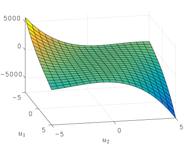
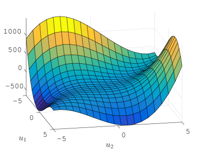
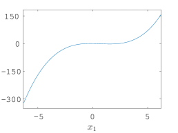
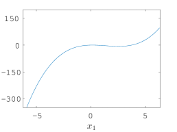
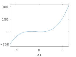
Figure 2: The decoupling problem in Example 1 consists of decomposing the multivariate functions $f_{1}(u_{1},u_{2})$ and $f_{2}(u_{1},u_{2})$ (top row) to the univariate functions $g_{1}(x_{1})$, $g_{2}(x_{2})$, and $g_{3}(x_{3})$ (bottom row), using suitable transformation matrices as in (1).

Remark 1.

In general, the coupled representation $\mathbf{f}(\mathbf{u})$ has $n\left({m+d\choose d}-1\right)$ coefficients, while the decoupled representation $\mathbf{W}\mathbf{g}(\mathbf{V}^{\top}\mathbf{u})$ has $r(m+n+d)$ coefficients. Due to the combinatorial increase of the number of coefficients in the coupled representation, the decoupled representation is especially beneficial for large values of $m$, $n$, and $d$. But even for small values of $m$, $n$, and $d$, the parametric reduction can be significant, for example, if $m=n=3$, $d=5$, and $r=3$, the coupled representation has 168 coefficients, while the decoupled one has only 36 coefficients.

3 Decoupling polynomials and symmetric tensor decompositions

Let us review some well-known facts that connect polynomials with symmetric tensors [35, 36], and that connect some special cases of the representation (1) with symmetric tensor decompositions.

3.1 Homogeneous polynomials, symmetric tensors and Waring decomposition

It is well-known that there is a one-to-one correspondence between homogeneous polynomials and symmetric tensors [35]. For instance, the polynomial $-8u_{1}^{2}-8u_{1}u_{2}-20u_{2}^{2}$ can be written as

$$-8u_{1}^{2}-8u_{1}u_{2}-20u_{2}^{2}=\mathbf{u}^{\top}\Psi^{(2)}\mathbf{u},\quad\mbox{where }\Psi^{(2)}=\left[\begin{array}[]{rr}-8&-4\\ -4&-20\end{array}\right].$$ (4)

In general, let $p^{(d)}(u_{1},\ldots,u_{m})$ be a homogeneous polynomial (also called a $d$-ary form) of degree $d$ in $m$ variables. Then there is a unique symmetric tensor $\Psi^{(d)}$ of order $d$ and dimension $m$ such that

$$p(\mathbf{u})=\Psi^{(d)}\bullet_{1}\mathbf{u}\cdots\bullet_{d}\mathbf{u}.$$ (5)

Next, it is easy to see that the decoupling problem for the polynomial (5) takes the form

$$p(u_{1},\ldots,u_{m})=\sum_{i=1}^{r}w_{i}(v_{1i}u_{1}+\cdots+v_{mi}u_{m})^{d},$$ (6)

which is known as the Waring decomposition [19, 20] of $p(u_{1},\ldots,u_{m})$. The Waring decomposition, in its turn, is equivalent to the symmetric CP decomposition of $\Psi^{(d)}$:

$$\Psi^{(d)}=\sum_{i=1}^{r}w_{i}(\mathbf{v}_{i}\circ\cdots\circ\mathbf{v}_{i}).$$

The symmetric CP decomposition of $\Psi^{(d)}$ reveals possible values for the unknowns $v_{ij}$ and $w_{i}$.

Example 2.

Consider the polynomial given in (4). Then the corresponding symmetric matrix $\Psi^{(2)}$ admits the decomposition

$$\left[\begin{array}[]{rr}-8&-4\\ -4&-20\end{array}\right]=\left[\begin{array}[]{rr}-2&2\\ 2&4\end{array}\right]\left[\begin{array}[]{rr}-1&0\\ 0&-1\end{array}\right]\left[\begin{array}[]{rr}-2&2\\ 2&4\end{array}\right],$$ (7)

such that $p(u_{1},u_{2})=\mathbf{u}^{\top}\Psi^{(2)}\mathbf{u}$ has the Waring decomposition

$$p(u_{1},u_{2})=-(-2u_{1}+2u_{2})^{2}-(2u_{1}+4u_{2})^{2}.$$

Notice that the symmetric decomposition of $\Psi^{(2)}$ from Example 2 is not unique (nor ‘essentially unique’ [2]). Indeed, the eigenvalue decomposition

$$\left[\begin{array}[]{rr}-8&-4\\ -4&-20\end{array}\right]\approx\left[\begin{array}[]{rr}0.2898&-0.9571\\ 0.9571&0.2898\end{array}\right]\left[\begin{array}[]{rr}-21.2111&0\\ 0&-6.7889\end{array}\right]\left[\begin{array}[]{rr}0.2898&0.9571\\ -0.9571&0.2898\end{array}\right]$$

provides another valid factorization. For $d>2$, however, the Waring decomposition (6) possesses uniqueness properties even in the case of quite large ranks [37, 38].

Along the same lines, it is possible to decouple jointly several homogeneous polynomials. Consider the case of $n$ homogeneous polynomials of degree $d$, denoted by

$$\begin{array}[]{rcl}p_{1}(u_{1},\ldots,u_{m})&=&\Psi^{(d)}_{1}\bullet_{1}\mathbf{u}\cdots\bullet_{d}\mathbf{u},\\ &\vdots&\\ p_{n}(u_{1},\ldots,u_{m})&=&\Psi^{(d)}_{n}\bullet_{1}\mathbf{u}\cdots\bullet_{d}\mathbf{u}.\\ \end{array}$$ (8)

Then the decoupling problem (1) corresponds to the simultaneous Waring decomposition of several forms or, equivalently, the coupled CP decomposition of several symmetric tensors. The rank and identifiability properties of simultaneous Waring decompositions were also studied in the literature, see [23, 37, 39] and references therein.

3.2 The case of non-homogeneous polynomials

Next, consider the case of non-homogeneous polynomials. Any non-homogeneous polynomial of degree $d$ can hence be written as

$$p(\mathbf{u})=\mathbf{u}^{\top}\Psi^{(1)}+\mathbf{u}^{\top}\Psi^{(2)}\mathbf{u}+\Psi^{(3)}\bullet_{1}\mathbf{u}\bullet_{2}\mathbf{u}\bullet_{3}\mathbf{u}+\cdots+\Psi^{(d)}\bullet_{1}\mathbf{u}\cdots\bullet_{d}\mathbf{u},$$ (9)

where $\Psi^{(1)}\in\mathbb{R}^{m}$ , $\Psi^{(2)}\in\mathbb{R}^{m\times m}$ is a symmetric matrix, and each $\Psi^{(s)}\in\mathbb{R}^{m\times\cdots\times m}$, $3\leq s\leq d$, is a symmetric tensor of order $s$.

Example 3.

We continue Example 1. We can write $f_{1}(u_{1},u_{2})$ and $f_{2}(u_{1},u_{2})$ as

$$f_{1}(u_{1},u_{2})=\mathbf{u}^{\top}\left[\begin{array}[]{r}3\\ 9\end{array}\right]+\mathbf{u}^{\top}\left[\begin{array}[]{rr}-8&-4\\ -4&-20\end{array}\right]\mathbf{u}+\Psi^{(3)}\bullet_{1}\mathbf{u}\bullet_{2}\mathbf{u}\bullet_{3}\mathbf{u},$$

with

$$\Psi^{(3)}_{:,:,1}=\left[\begin{array}[]{rr}-3&-3\\ -3&-9\end{array}\right],\quad\quad\quad\Psi^{(3)}_{:,:,2}=\left[\begin{array}[]{rr}-3&-9\\ -9&-15\end{array}\right],$$

and

$$f_{2}(u_{1},u_{2})=\mathbf{u}^{\top}\left[\begin{array}[]{r}0\\ -3\end{array}\right]+\mathbf{u}^{\top}\left[\begin{array}[]{rr}10&8\\ 8&10\end{array}\right]\mathbf{u}+\Psi^{(3)}\bullet_{1}\mathbf{u}\bullet_{2}\mathbf{u}\bullet_{3}\mathbf{u},$$

with

$$\Psi^{(3)}_{:,:,1}=\left[\begin{array}[]{rr}-7&-2\\ -2&2\end{array}\right],\quad\quad\quad\Psi^{(3)}_{:,:,2}=\left[\begin{array}[]{rr}-2&2\\ 2&7\end{array}\right].$$

The decomposition of a single non-homogeneous polynomial as in (3) is hence equivalent to joint decomposition of several symmetric tensors but of different orders [32].

Finally, several non-homogeneous polynomials can be jointly decomposed in a similar way. Consider $n$ non-homogeneous polynomials of maximal degree $d$, denoted as

$$\begin{array}[]{rcl}p_{1}(u_{1},\ldots,u_{m})&=&\mathbf{u}^{\top}\Psi^{(1)}_{1}+\cdots+\Psi^{(d)}_{1}\bullet_{1}\mathbf{u}\cdots\bullet_{d}\mathbf{u},\\ &\vdots&\\ p_{n}(u_{1},\ldots,u_{m})&=&\mathbf{u}^{\top}\Psi^{(1)}_{n}+\cdots+\Psi^{(d)}_{n}\bullet_{1}\mathbf{u}\cdots\bullet_{d}\mathbf{u},\end{array}$$ (10)

The full decomposition in (1) can be also viewed as a coupled tensor decomposition, which will be presented in Section 6.2.

4 Tensorizations and their decompositions

In this section, we recall tensorizations proposed in the literature to find the decomposition (1) by a CP decomposition of a single tensor constructed from $\mathbf{f}$, namely the tensorizations of [26] and [24]. We recall basic properties and give short proofs for completeness, although these proofs are already present in [26, 24]. We also use a slightly different notation to simplify the exposition.

4.1 Tensor of unfoldings [26]

The above link between polynomials, (partially) symmetric tensors and their CP decompositions gives rise to the tensorization approach of [26], in which a tensor is constructed from the coefficients of the polynomials $f_{1}(u_{1},\ldots,u_{m})$ up to $f_{n}(u_{1},\ldots,u_{m})$. This tensorization offers the advantage that several polynomials can be represented as a single tensor, and the decoupling task can be solved using a single (but structured) CP decomposition. In this approach, the tensor (shown in Figure 3) is constructed from the coefficients of the polynomial map of degree $d$, as follows:

• The tensor has size $n\times m\times\delta$, where $\delta=\sum\limits_{k=1}^{d}m^{k-1}$.

• The tensor is constructed by slices

  $$\mathcal{Q}_{i,:,:}:=\Psi(f_{i}),$$

  where $\Psi$ is a structured $m\times\delta$ matrix built from the coefficients of $f_{i}(\mathbf{u})$.

Figure 3: The coefficients of a polynomial map $\mathbf{f}:\mathbb{R}^{m}\to\mathbb{R}^{n}$ of degree $d$ can be arranged into an $n\times m\times\delta$ tensor $\mathcal{Q}$, where $\delta=\sum_{k=1}^{d}m^{k-1}$.

Now let us describe the construction of the structured coefficient matrix $\Psi(p)$ for a given polynomial of degree $d$. Recall that each such polynomial can be written as in (9), where $\Psi^{(1)}\in\mathbb{R}^{m}$ , $\Psi^{(2)}\in\mathbb{R}^{m\times m}$ is a symmetric matrix and $\Psi^{(s)}\in\mathbb{R}^{m\times\cdots\times m}$ are symmetric tensors of order $s$. Then the matrix $\Psi(p)\in\mathbb{R}^{m\times\delta}$ is constructed as

$$\Psi(p)=\left[\begin{array}[]{c|c|c|c|c}\Psi^{(1)}&\Psi^{(2)}&\Psi^{(3)}_{(1)}&\cdots&\Psi^{(d)}_{(1)}\end{array}\right],$$ (11)

where $\mathcal{G}_{(1)}$ denotes the first-mode unfolding of a tensor $\mathcal{G}$.

Example 4.

A third-degree polynomial in two variables

$$p(u_{1},u_{2})=a_{1}u_{1}+a_{2}u_{2}+b_{1}u_{1}^{2}+2b_{2}u_{1}u_{2}+b3u_{2}^{2}+d_{1}u_{1}^{3}+3d_{2}u_{1}^{2}u_{2}+3d_{3}u_{1}u_{2}^{2}+d_{4}u_{3}^{3}$$

has the representation

$$p(u_{1},u_{2})=\mathbf{u}^{\top}\begin{bmatrix}a_{1}\\ a_{2}\end{bmatrix}+\mathbf{u}^{\top}\begin{bmatrix}b_{1}&b_{2}\\ b_{2}&b_{3}\end{bmatrix}\mathbf{u}+\Psi^{(3)}\bullet_{1}\mathbf{u}\bullet_{2}\mathbf{u}\bullet_{3}\mathbf{u},$$ (12)

where

$$\Psi^{(3)}_{:,:,1}=\begin{bmatrix}d_{1}&d_{2}\\ d_{2}&d_{3}\end{bmatrix},\quad\Psi^{(3)}_{:,:,2}=\begin{bmatrix}d_{2}&d_{3}\\ d_{3}&d_{4}\end{bmatrix}.$$

By putting all the unfoldings together, we get

$$\Psi(p)=\left[\begin{array}[]{c|cc|cccc}a_{1}&b_{1}&b_{2}&d_{1}&d_{2}&d_{2}&d_{3}\\ a_{2}&b_{2}&b_{3}&d_{2}&d_{3}&d_{3}&d_{4}\end{array}\right].$$ (13)

Hence, for $f_{1}$ and $f_{2}$ in Example 1, the slices of the tensor $\mathcal{Q}$ are given by

$$\mathcal{Q}_{1,:,:}=\Psi(f_{1})=\left[\begin{array}[]{c|cc|cccc}3&-8&-4&-3&-3&-3&-9\\ 9&-4&-20&-3&-9&-9&-15\end{array}\right],$$

and

$$\mathcal{Q}_{2,:,:}=\Psi(f_{2})=\left[\begin{array}[]{c|cc|cccc}0&10&8&-7&-2&-2&2\\ -3&8&10&-2&2&2&7\end{array}\right].$$

As proved in [26], the tensor $\mathcal{Q}$ has a CP decomposition, which reveals the decomposition (1). We repeat here a simplified version of the proof for completeness.

Lemma 1.

For the polynomial map (1), the tensor $\mathcal{Q}$ has the following CP decomposition:

$$\mathcal{Q}=\sum\limits_{k=1}^{r}\mathbf{w}_{k}\circ\mathbf{v}_{k}\circ\mathbf{z}_{k},$$ (14)

where

$$\mathbf{z}_{k}=\left[\begin{array}[]{c|c|c|c|c}c_{k,1}&c_{k,2}\mathbf{v}_{k}^{\top}&c_{k,3}(\mathbf{v}_{k}\otimes\mathbf{v}_{k})^{\top}&\cdots&c_{k,d}(\mathbf{v}_{k}\otimes\cdots\otimes\mathbf{v}_{k})^{\top}\end{array}\right]^{\top}.$$ (15)

Proof.

Consider $q_{k}(\mathbf{u}):=g_{k}(\mathbf{v}_{k}^{\top}\mathbf{u})$, where $g_{k}$ is as in (2). Easy calculations show that

$$\Psi(q_{k})=\mathbf{v}_{k}\mathbf{z}^{\top}_{k},$$

see also [40, eqn. (A.7)]. Since, from (3) $f_{i}(\mathbf{u})=\sum\limits_{k=1}^{r}(\mathbf{w}_{k})_{i}q_{k}(\mathbf{u})$, we have that

$$\Psi(f_{i})=\sum\limits_{k=1}^{r}(\mathbf{w}_{k})_{i}\mathbf{v}_{k}\mathbf{z}^{\top}_{k}$$

which implies (14). ∎

Example 5.

We continue Examples 1, 4. The Kronecker products of columns of $\mathbf{V}$ are:

$$(\mathbf{v}_{1}\otimes\mathbf{v}_{1})^{\top}=\begin{bmatrix}4&2&2&1\end{bmatrix},(\mathbf{v}_{2}\otimes\mathbf{v}_{2})^{\top}=\begin{bmatrix}1&-1&-1&1\end{bmatrix},(\mathbf{v}_{3}\otimes\mathbf{v}_{3})^{\top}=\begin{bmatrix}1&2&2&4\end{bmatrix}.$$

Hence, the matrix $\mathbf{Z}=\begin{bmatrix}\mathbf{z}_{1}&\mathbf{z}_{2}&\mathbf{z}_{3}\end{bmatrix}$ is given by

$$\mathbf{Z}^{\top}=\left[\begin{array}[]{c|cc|cccc}-1&-4&-2&4&2&2&1\\ 1&4&-4&1&-1&-1&1\\ -2&2&4&1&2&2&4\\ \end{array}\right].\\$$

4.2 The tensor of Jacobian matrices of [24]

The tensorization method of [24] does not use the coefficients of $\mathbf{f}(\mathbf{u})$ directly, but proceeds by collecting the first-order information of $\mathbf{f}(\mathbf{u})$ (i.e., the partial derivatives) in a set of sampling points. The thusly obtained Jacobian matrices are arranged into a third-order tensor, of which the CP decomposition reveals the decomposition (1).

As in [24], we consider the Jacobian of $\mathbf{f}$:

$$\mathbf{J}_{\mathbf{f}}(\mathbf{u}):=\begin{bmatrix}\frac{\partial f_{1}}{\partial u_{1}}(\mathbf{u})&\cdots&\frac{\partial f_{1}}{\partial u_{m}}(\mathbf{u})\\ \vdots&&\vdots\\ \frac{\partial f_{n}}{\partial u_{1}}(\mathbf{u})&\cdots&\frac{\partial f_{n}}{\partial u_{m}}(\mathbf{u})\end{bmatrix}.$$ (16)

Using Lemma 2, the tensorization is constructed as follows (see Figure 4):

• $N$ points $\mathbf{u}^{(1)},\ldots,\mathbf{u}^{(N)}\in\mathbb{R}^{m}$ are chosen (so-called sampling points).

• An $n\times m\times N$ tensor $\mathcal{J}$ is constructed by stacking the Jacobian evaluations at $\mathbf{u}^{(k)}$

  $$\mathcal{J}_{:,:,k}:=\mathbf{J}_{\mathbf{f}}(\mathbf{u}^{(k)}).$$

Figure 4: The third-order tensor $\mathcal{J}$ is constructed by stacking behind each other a set of Jacobian matrices $\mathbf{J}$ evaluated at the sampling points $\mathbf{u}^{(k)}$. Its CP decomposition is equivalent to joint matrix diagonalization of the Jacobian matrix slices.

Example 6.

We continue Example 1. As a set of sampling points, we choose

$$\mathbf{u}=\begin{bmatrix}0\\ 0\end{bmatrix},\mathbf{u}^{(2)}=\begin{bmatrix}1\\ 0\end{bmatrix},\mathbf{u}^{(3)}=\begin{bmatrix}0\\ 1\end{bmatrix}.$$

By evaluating $\mathbf{J}_{\mathbf{f}}(\mathbf{u})$ at these points, we get the tensor $\mathcal{J}$ given by

$$\mathcal{J}_{:,:,1}=\begin{bmatrix}3&9\\ 0&-3\end{bmatrix},\quad\mathcal{J}_{:,:,2}=\begin{bmatrix}-22&-8\\ -1&7\end{bmatrix},\quad\mathcal{J}_{:,:,3}=\begin{bmatrix}-32&-76\\ 22&38\end{bmatrix}.$$ (17)

If $\mathbf{f}(\mathbf{u})$ has a decoupled representation (1), the following lemma holds true.

Lemma 2 ([24, Lemma 2.1]).

The first order derivatives of (1) are given by

$$\mathbf{J}_{\mathbf{f}}(\mathbf{u})=\mathbf{W}\mathop{\operator@font diag}(g^{\prime}_{1}(\mathbf{v}_{1}^{\top}\mathbf{u}),\ldots,g^{\prime}_{r}(\mathbf{v}_{r}^{\top}\mathbf{u}))\mathbf{V}^{\top},$$ (18)

where $g_{i}^{\prime}(t):=\frac{dg_{i}}{dt}(t)$.

The proof, given in [24], follows by chain rule:

$$\mathbf{J}_{\mathbf{f}}(\mathbf{u})=\mathbf{W}\mathbf{J}_{\mathbf{g}}(\mathbf{V}^{\top}\mathbf{u})\mathbf{V}^{\top}.$$

By Lemma 2, the evaluations of the Jacobians can be jointly factorized:

$$\begin{split}\mathbf{J}(\mathbf{u}^{(1)})&=\mathbf{W}\mathbf{D}^{(1)}\mathbf{V}^{\top},\\ &\;\vdots\\ \mathbf{J}(\mathbf{u}^{(N)})&=\mathbf{W}\mathbf{D}^{(N)}\mathbf{V}^{\top},\end{split}$$ (19)

where $\mathbf{D}^{(k)}=\mathop{\operator@font diag}(g^{\prime}_{1}(\mathbf{v}_{1}^{\top}\mathbf{u}^{(k)}),\ldots,g^{\prime}_{r}(\mathbf{v}_{r}^{\top}\mathbf{u}^{(k)}))$. Therefore, $\mathcal{J}$ admits a CP decomposition

$$\mathcal{J}=\llbracket\mathbf{W},\mathbf{V},\mathbf{H}\rrbracket=\sum\limits_{k=1}^{r}\mathbf{w}_{k}\circ\mathbf{v}_{k}\circ\mathbf{h}_{k},$$ (20)

where $\mathbf{w}_{k}$, $\mathbf{v}_{k}$ are as in (3), and $\mathbf{h}_{k}$ contains the evaluations of $g^{\prime}_{k}(\mathbf{v}_{k}^{\top}\mathbf{u})$ in $\mathbf{u}^{(1)},\ldots,\mathbf{u}^{(N)}$:

$$\mathbf{h}_{k}=\begin{bmatrix}g^{\prime}_{k}(\mathbf{v}_{k}^{\top}\mathbf{u}^{(1)})&\cdots&g^{\prime}_{k}(\mathbf{v}_{k}^{\top}\mathbf{u}^{(N)})\end{bmatrix}^{\top}.$$ (21)

Example 7.

We continue Examples 1 and 6. By differentiation, we get

$$\begin{split}g^{\prime}_{1}(t)=3t^{2}-4t-1,\quad g^{\prime}_{2}(t)=3t^{2}-8t+1,\quad g^{\prime}_{3}(t)=3t^{2}+4t-2,\end{split}$$

and hence, by substitution,

$$\mathbf{H}=\left[\begin{array}[]{rrr}-1&1&-2\\ 3&12&5\\ -2&-4&18\end{array}\right].$$ (22)

Straightforward calculations show indeed that $\mathcal{J}$ given in (17) admits a decomposition (20) with $\mathbf{H}$ as in (22).

5 Relation between tensorizations $\mathcal{J}$ and $\mathcal{Q}$

In this section, we show how CP decompositions of (14) and (20) are related. Moreover, we establish the relation between the ranks of the tensors and uniqueness of CP decompositions.

First, we show the relation between the vectors $\mathbf{z}_{k}$ and $\mathbf{h}_{k}$, defined in (15) and (21), respectively. We give the proof of this basic fact for completeness.

Lemma 3.

The vectors $\mathbf{z}_{k}$ and $\mathbf{h}_{k}$ defined in (15) and (21), respectively, satisfy

$$\mathbf{h}_{k}=\mathbf{A}^{\top}\mathbf{z}_{k},$$ (23)

where $\mathbf{A}\in\mathbb{R}^{\delta\times N}$ is a Vandermonde-like matrix whose columns are

$$\mathbf{A}_{:,j}=\left[\begin{array}[]{c|c|c|c|c}1&2(\mathbf{u}^{(j)})^{\top}&3(\mathbf{u}^{(j)}\otimes\mathbf{u}^{(j)})^{\top}&\cdots&d(\mathbf{u}^{(j)}\otimes\cdots\otimes\mathbf{u}^{(j)})^{\top}\end{array}\right]^{\top}.$$ (24)

Proof.

Recall that by the properties of the Kronecker product

$$(\underbrace{\mathbf{u}\otimes\cdots\otimes\mathbf{u}}_{d\text{ times }})^{\top}(\mathbf{v}\otimes\cdots\otimes\mathbf{v})=(\mathbf{u}^{\top}\mathbf{v})^{d}.$$

Then from (15) have that

$$(\mathbf{A}^{\top}\mathbf{z}_{k})_{j}=\mathbf{A}_{:,j}^{\top}\mathbf{z}_{k}=c_{k,1}+c_{k,2}(\mathbf{v}_{k}^{\top}\mathbf{u}^{(j)})+\cdots+c_{k,d}(\mathbf{v}_{k}^{\top}\mathbf{u}^{(j)})^{d-1}=(\mathbf{h}_{k})_{j},$$

where the last equality follows from (21) and the fact that

$$g^{\prime}_{k}(t)=c_{k,1}+c_{k,2}t+\cdots+c_{k,d}t^{d-1}.$$

∎

Example 8.

In Example 6, the matrix $\mathbf{A}$ can be found as

$$\mathbf{A}^{\top}=\left[\begin{array}[]{c|cc|cccc}1&0&0&0&0&0&0\\ 1&2&0&3&0&0&0\\ 1&0&2&0&0&0&3\\ \end{array}\right].$$

It is easy to see that $\mathbf{H}=\mathbf{A}^{\top}\mathbf{Z}$.

As a consequence, we get that the two tensors and their ranks are also related.

Theorem 1.

1. For any polynomial map $\mathbf{f}$, $\mathcal{J}$ and $\mathcal{Q}$ are related as

   $$\mathcal{J}=\mathcal{Q}\bullet_{3}\mathbf{A}^{\top}.$$ (25)

2. The rank of $\mathbf{A}$ is bounded as

   $$\mathop{\operator@font rank}\mathbf{A}\leq M:=\binom{m+d-1}{d-1}.$$

   In addition, if $M\leq N$, and $M$ points in $\{\mathbf{u}^{(j)}\}$ are in general position, then $\mathop{\operator@font rank}\mathbf{A}=M$. For example, if points $\{\mathbf{u}^{(j)}\}$ are independent and sampled from a continuous probability distribution, then $\mathop{\operator@font rank}\mathbf{A}=M$ with probability $1$.

3. If $\mathbf{A}$ has maximal possible rank (i.e. $\mathop{\operator@font rank}\mathbf{A}=M$), then

   $$\mathop{\operator@font rank}\mathcal{J}=\mathop{\operator@font rank}\mathcal{Q},$$

   and all the minimal CP decompositions differ only by the third factors, which are linked as in (23). Moreover, if the CP decomposition of $\mathcal{Q}$ is unique, then the CP decomposition of $\mathcal{J}$ is also unique.

Proof of Lemma 3.

Let us express $g^{\prime}_{k}(\mathbf{v}_{k}^{\top}\mathbf{u})$ in an explicit form. First, $g^{\prime}_{k}(t)=c_{k,1}+2c_{k,2}t+3c_{k,3}t^{2}+\cdots+dc_{k,d}t^{d-1}$, from which it follows that

$$g^{\prime}_{k}(\mathbf{v}_{k}^{\top}\mathbf{u})=c_{k,1}+2c_{k,2}\mathbf{v}_{k}^{\top}\mathbf{u}+3c_{k,3}(\mathbf{v}_{k}^{\top}\mathbf{u})^{2}+\cdots+dc_{k,d}(\mathbf{v}_{k}^{\top}\mathbf{u})^{d-1}.$$

Since $(\mathbf{v}^{\top}\mathbf{u})^{s}=(\mathbf{v}\otimes\cdots\otimes\mathbf{v})^{\top}(\mathbf{u}\otimes\cdots\otimes\mathbf{u})$, the $j$-th element of $\mathbf{h}_{k}$ is equal to

$$(\mathbf{h}_{k})_{j}=h_{j,k}=g^{\prime}_{k}(\mathbf{v}_{k}^{\top}\mathbf{u}^{(j)})=\mathbf{A}_{:,k}^{\top}\mathbf{z}_{k},$$

which completes the proof. ∎

Proof of Theorem 1.

1. First, any polynomial map $\mathbf{f}$ can be decomposed as (1) with $r$ sufficiently large. Let us take such a decomposition; then it holds that

$$(\mathcal{Q})\bullet_{3}\mathbf{A}^{\top}=\left(\sum\limits_{k=1}^{r}\mathbf{w}_{k}\circ\mathbf{v}_{k}\circ\mathbf{z}_{k}\right)\bullet_{3}\mathbf{A}^{\top}=\sum\limits_{k=1}^{r}\mathbf{w}_{k}\circ\mathbf{v}_{k}\circ\mathbf{A}^{\top}\mathbf{z}_{k}=\mathcal{J},$$

where the last equality follows from (23).

2. By construction, each element in the image of $\mathbf{A}$ lies in the following subspace:

$$\begin{split}\mathscr{A}:=\{&\begin{bmatrix}a_{0}&\mathbf{a}_{1}^{\top}&\mathbf{a}_{2}^{\top}&\cdots&\mathbf{a}_{d-1}^{\top}\end{bmatrix}^{\top}\in\mathbb{R}^{\delta}|\\ &\mathbf{a}_{k}\in\mathbb{R}^{n^{k}}\mbox{ is a vectorization of a symmetric }m\times\cdots\times m\mbox{ tensor}.\}\end{split}$$ (26)

Taking into account that the dimension of the space of $m\times\cdots\times m$ symmetric tensors of order $s$ is $\binom{m+s-1}{s}$, we get that the maximal possible rank of $\mathbf{A}$ is

$$1+m+\binom{m+1}{2}+\dots\binom{m+d-2}{d-1}=M.$$

Next, from (24), we have that the $k$-th column contains evaluations of all $M$ monomials $\{u^{j_{1}}_{1}\cdots u^{j_{m}}_{m}\leq d-1\}^{j_{1}+\cdots+j_{m}\leq d}_{j_{1},\ldots,j_{m}=0}$ at a point $\mathbf{u}^{(k)}$ (scaled by a constant). If, without loss of generality, the first $M$ points $\{\mathbf{u}^{(k)}\}_{k=1}^{M}$ are in general position, then the columns of $\mathbf{A}$ corresponding to different monomials are linearly independent by [41, Multiplicity One Theorem], hence $\mathop{\operator@font rank}\mathbf{A}=M$.

3. Note that each tube $\mathcal{Q}_{i,j,:}$ of the tensor $\mathcal{Q}$, by construction, lies in $\mathscr{A}$. If $\mathop{\operator@font rank}\mathbf{A}=M$, then its row span coincides with $\mathscr{A}$. Hence the following identity holds true:

$$\mathcal{J}\bullet_{3}(\mathbf{A}^{\dagger})^{\top}=\mathcal{Q}\bullet_{3}(\mathbf{A}\mathbf{A}^{\dagger})^{\top}=\mathcal{Q}.$$ (27)

The remaining properties follow from (27) and (25). ∎

6 Structured tensor decompositions

6.1 From CPD to a decomposition with structured rank-one terms

The CP decomposition of $\mathcal{J}$ and $\mathcal{Q}$, although related, are not always equivalent to the original decomposition (3). This happens because there are still nontrivial linear dependencies between the elements of $\mathcal{Q}$ and $\mathcal{J}$. In what follows, we establish relationships between the CP decompositions and the original decomposition (3).

First, we prove that for the rank-one case, these decompositions coincide.

Proposition 1.

Consider a polynomial map $\mathbf{f}(\mathbf{u})$ of degree $d$, and the tensor $\mathcal{Q}$ built from it. Then the following holds

$$\mathop{\operator@font rank}(\mathcal{Q})\leq 1\iff\mathbf{f}(\mathbf{u})=\mathbf{w}g(\mathbf{v}^{\top}\mathbf{u}),$$

where $\mathbf{w}\in\mathbb{R}^{n}$, $\mathbf{v}\in\mathbb{R}^{m}$ and $g(t)$ is a polynomial of degree $d$.

Proof.

The $\boxed{\Leftarrow}$ follows from Lemma 1. Let us prove the $\boxed{\Rightarrow}$ part. Assume that

$$\mathcal{Q}=\mathbf{w}\circ\mathbf{v}\circ\mathbf{y}.$$

First, since the tensor $\mathcal{Q}$ contains all the coefficients of the derivatives, we have that there exists a polynomial $\widetilde{f}(\mathbf{u})$ such that $\nabla f_{k}(\mathbf{u})=(\mathbf{w})_{k}\nabla\widetilde{f}(\mathbf{u})$. Since the polynomials $f_{k}(\mathbf{u})$ do not have constant terms, we have that

$$\mathbf{f}(\mathbf{u})=\mathbf{w}\widetilde{f}(\mathbf{u}),$$

where $\Psi(\widetilde{f})=\mathbf{v}\mathbf{y}^{\top}$.

Next, let us show that the polynomial $\widetilde{f}$ should necessarily the form $\widetilde{f}(\mathbf{u})={g}(\mathbf{v}^{\top}\mathbf{u})$. Since $\Psi(\widetilde{f})=\mathbf{v}\mathbf{y}^{\top}$, then it follows from (11) that all the unfoldings $\Psi^{(1)}$, $\Psi^{(2)}$, $\Psi^{(3)}_{(1)},\cdots,\Psi^{(d)}_{(1)}$ have rank at most one and their column space is spanned by the vector $\mathbf{v}$. Therefore, we have that

$$\begin{split}&\Psi^{(1)}=c_{1}\mathbf{v},\\ &\Psi^{(2)}=c_{2}\mathbf{v}\mathbf{v}^{\top},\\ &\Psi^{(3)}=c_{3}\mathbf{v}\circ\mathbf{v}\circ\mathbf{v},\\ &\vdots\\ &\Psi^{(d)}=c_{d}\mathbf{v}\circ\cdots\circ\mathbf{v},\\ \end{split}$$

and hence $\widetilde{f}(\mathbf{u})={g}(\mathbf{v}^{\top}\mathbf{u})$ where

$${g}(t)={c}_{1}t+{c}_{2}t^{2}+\cdots+{c}_{d}t^{d},$$

which completes the proof. ∎

Remark 2.

The fact that $\mathop{\operator@font rank}\Psi(\widetilde{f})\leq 1$ implies $\widetilde{f}(\mathbf{u})=g(\mathbf{v}^{\top}\mathbf{u})$ also can be proved alternatively, by noting that the matrix $\Psi{\widetilde{f}}$, after removing duplicate columns, can be reduced to the form $S(f)$ in [33, Proposition 22]. Hence, by [33, Proposition 4.1], the polynomial $\widetilde{f}$ has necessarily the form $\widetilde{f}(\mathbf{u})=g(\mathbf{v}^{\top}\mathbf{u})$. However, this alternative proof requires introducing extra notation, which would be much longer that the proof presented in this paper.

Corollary 1.

If the $N$ sampling points are chosen such that the $\mathop{\operator@font rank}(\mathbf{A})=M$, then

$$\mathop{\operator@font rank}(\mathcal{J})\leq 1\iff\mathbf{f}(\mathbf{u})=\mathbf{w}g(\mathbf{v}^{\top}\mathbf{u}).$$

As a corollary of Proposition 1, we get that the original polynomial decomposition (3) is equivalent to a structured CP decomposition.

Corollary 2.

Let $\mathcal{L}_{\mathcal{Q}}\subset\mathbb{R}^{n\times m\times\delta}$ be the linear subspace of tensors with the structure of $\mathcal{Q}$. Let the sampling points be chosen such that $\mathop{\operator@font rank}\mathbf{A}=M$, and $\mathcal{L}_{\mathcal{J}}\subset\mathbb{R}^{n\times m\times N}$ be the linear subspace of tensors with the structure of $\mathcal{J}$.

Then the following three statements are equivalent:

1. the polynomial map $\mathbf{f}(\mathbf{u})$ admits a decomposition (3);

2. the tensor $\mathcal{Q}(\mathbf{f})$ admits the structured CP decomposition

   $$\mathcal{Q}=\mathcal{Q}_{1}+\cdots+\mathcal{Q}_{r},\quad\mathop{\operator@font rank}(\mathcal{Q}_{k})=1,\quad\mathcal{Q}_{k}\in\mathcal{L}_{\mathcal{Q}};$$ (28)

3. the tensor $\mathcal{J}(\mathbf{f})$ admits the structured CP decomposition

   $$\mathcal{J}=\mathcal{J}_{1}+\cdots+\mathcal{J}_{r},\quad\mathop{\operator@font rank}(\mathcal{J}_{k})=1,\quad\mathcal{J}_{k}\in\mathcal{L}_{\mathcal{J}}.$$ (29)

The structure constraint is important: indeed, the CP decomposition of the tensor $\mathcal{Q}$ or $\mathcal{J}$ is not necessarily structured. In general, we do not know even if the CP rank is equal to the structured CP rank (minimal number of terms in (28) or (29)). This is similar to the Comon’s conjecture [35, §5] about symmetric tensors: it is not known whether the symmetric rank of a symmetric tensor equals its non-symmetric rank.

However, if the CP decomposition of a tensor is unique (for example, if it satisfies Kruskal’s uniqueness conditions), then it should necessarily be a structured CP decomposition.

6.2 Computing coupled/structured CP decomposition

Earlier attempts to tackle the structured case were made by [25, 13] and [42, §8, pp. 133–136]. The attempts of [25, 13] have the disadvantage that a tensor is built that has missing values, which increase in number as the polynomial degree grows. The attempt of [42] consisted of parameterizing the internal nonlinear functions $g_{k}$ using their coefficients. Although this seems a promising approach, it turned out to be problematic in practice to build a working algorithm, as the decoupling method led to strongly nonlinear/nonconvex optimization problems.

We propose to tackle the problem by solving a coupled and structured CP decomposition instead. First, let us consider simultaneous decoupling of homogeneous polynomials (8). Let us arrange the $\Psi^{(d)}_{i}$, for $i=1,\ldots,n$ into a tensor $\mathcal{T}^{d}$, such that $\mathcal{T}^{d}_{i,:,\ldots,:}=\Psi^{(d)}_{i}$, for all $i=1,\ldots,n$. Then it is easy to verify that $\mathcal{T}^{d}$ admits a partially symmetric CP decomposition

$$\mathcal{T}^{d}=\llbracket\mathbf{W},\underbrace{\mathbf{V},\ldots,\mathbf{V}}_{\mbox{$d$ times}}\rrbracket,$$

which, in our decoupled representation (1), takes the form $\mathbf{W}\mathbf{g}(\mathbf{V}^{\top}\mathbf{u})$, where $\mathbf{g}(\mathbf{x})=\left[\begin{array}[]{ccc}x_{1}^{d}&\cdots&x_{r}^{d}\end{array}\right]^{\top}$.

Decoupling non-homogeneous polynomials can be achieved by means of a coupled structured CP decomposition of the $\mathcal{T}^{d}$ tensors. Let us arrange all $\Psi^{(d)}_{i}$, for $i=1,\ldots,n$ into the tensors $\mathcal{T}^{d}$ (like in the previous paragraph), such that $\mathcal{T}^{d}_{i,:,\ldots,:}=\Psi^{(d)}_{i}$, for all $i=1,\ldots,n$. We now have for each degree a coupled partially symmetric CP decomposition as

$$\begin{array}[]{rcl}\mathcal{T}^{1}&=&\llbracket\mathbf{W},\mathbf{V},\mathbf{c}_{1}^{\top}\rrbracket,\\ \mathcal{T}^{2}&=&\llbracket\mathbf{W},\mathbf{V},\mathbf{V},\mathbf{c}_{2}^{\top}\rrbracket,\\ &\vdots&\\ \mathcal{T}^{d}&=&\llbracket\mathbf{W},\underbrace{\mathbf{V},\ldots,\mathbf{V}}_{\mbox{$d$ times}},\mathbf{c}_{d}^{\top}\rrbracket,\end{array}$$ (30)

where the $\mathbf{c}_{i}$, for $i=1,\ldots,d$, are the $i$-th degree coefficients for each of the $r$ nonlinear functions $g_{k}$.

Remark that these coefficients were not required in the previous paragraphs when homogeneous polynomials were considered: in such cases the nonlinear functions $g_{k}$ are of the form $c_{k}t^{d}$, i.e., they differ only by a scaling factor, which can be assumed to be fully absorbed by $\mathbf{W}$. Also remark that there are redundancies in the representation (30): for example, an equivalent problem can be obtained if one rescales a coefficient vector $\mathbf{c}_{\delta}$ to a vector containing ones, in which case a rescaling has to take place on the remaining coefficients as well as on $\mathbf{W}$. Finally we want to mention that the framework of structured data fusion [43, 27] allows for computing tensor decompositions as in (30), where several tensors (and possibly matrices) are jointly decomposed while sharing factors, possibly while imposing structure on the factors.

Example 9.

Let us continue with Examples 1, 6 and 7. We have that $m=n=2$ and $r=3$, which does not guarantee a unique CP decomposition of $\mathcal{J}$ (under assumptions of genericity, see [24]). Indeed, if we compute a numerical CP decomposition of tensor $\mathcal{J}$, we find that, up to a relative norm-wise error $2.3546\times 10^{-16}$, $\mathcal{J}$ admits a CP decomposition with factors

$$\begin{array}[]{rcl}\tilde{\mathbf{W}}&=&\left[\begin{array}[]{rrr}1.1628&-3.2951&3.0252\\ 0.5705&1.1349&-2.1791\\ \end{array}\right],\quad\tilde{\mathbf{V}}=\left[\begin{array}[]{rrr}3.5822&-0.7705&-2.2959\\ -0.0226&-3.4455&-2.9785\\ \end{array}\right],\\ \\ \tilde{\mathbf{H}}&=&\left[\begin{array}[]{rrr}0.2736&0.8181&0.0312\\ -3.3900&0.2647&1.2313\\ 0.5334&-3.9194&3.4945\\ \end{array}\right],\\ \end{array}$$

the columns of which are not scaled and permuted versions of the columns of $\mathbf{W}$, $\mathbf{V}$, $\mathbf{H}$.

It can be shown that the ‘structured CP’ approaches are able to correctly return the underlying factors $\mathbf{W}$, $\mathbf{V}$ and $\mathbf{H}$ (up to scaling and permutation invariances). For instance, the structured data fusion framework [43, 27] is able to compute the coupled and partially symmetric decomposition (30). This returns

$$\begin{array}[]{rcl}\tilde{\mathbf{W}}&=&\left[\begin{array}[]{rrr}1.2767&1.7112&0\\ 0&-0.8556&-1.9980\end{array}\right],\quad\tilde{\mathbf{V}}=\left[\begin{array}[]{rrr}-0.9218&-1.0534&1.5879\\ 0.9218&-2.1067&0.7940\end{array}\right],\end{array}$$

as well as computed values for the coefficient vectors of $g_{i}(x_{i})$, which are omitted here. It can be verified that $\tilde{\mathbf{W}}$ and $\tilde{\mathbf{V}}$ are scaled and permuted versions of $\mathbf{W}$ and $\mathbf{V}$.

Remark that if one uses $m=n=r=2$, both the structured and non-structured CP decomposition return the same decomposition (up to scaling and permutation of the columns of the factors). Indeed, in this case, uniqueness is guaranteed (generically), ensuring that the underlying factors are identifiable. This could be checked easily by generating a variation of the equations that we are decoupling where the third columns of $\mathbf{V}$ and $\mathbf{W}$ are removed, so that $g_{3}(x_{3})$ is not considered.

6.3 Linking $\mathcal{Q}$ and $\mathcal{T}^{1},\ldots,\mathcal{T}^{d}$ tensors

In this section, we show how $\mathcal{Q}$ and its CPD is connected with the tensors $\mathcal{T}^{s}$ and their joint decomposition (30). Let $(1,2)$-reshapings of the tensors $\mathcal{T}^{s}$ to be the third order tensors $\mathcal{T}^{s}_{(1,2)}\in\mathbb{R}^{n\times m\times m^{s-1}}$ defined as

$$(\mathcal{T}^{s}_{(1,2)})_{i,j,:}=\mathop{\operator@font vec}(\mathcal{T}^{s}_{i,j,:,\cdots,:}).$$

Then it is easy to see that the tensor $\mathcal{T}^{s}_{(1,2)}$ can be split into slices as shown in Fig. 5, where the $\Psi^{(s,j)}$ is the symmetric tensor corresponding to the $s$-th degree homogeneous part of the polynomial $f_{k}$.

Figure 5: The slices of the tensor $\mathcal{T}^{s}$ are the unfoldings of the symmetric tensors corresponding to $s$-degree homogeneous parts of polynomials $f_{1},\ldots,f_{n}$.

By taking into account the definition (11) of the slices of the tensor $\mathcal{Q}$, we can easily see that $\mathcal{Q}$ can be constructed by stacking the tensors is equivalent to reshaping the tensors $\mathcal{T}^{s}_{(1,2)}$ along the third mode together, as shown in Fig. 6.

Figure 6: Stacking the reshapings of $\mathcal{T}^{s}$ together.

Remark that in Lemma 1 we see that the structure appearing in the CP decomposition of $\mathcal{Q}$ is closely connected to the simultaneous decomposition described in Section 6.2. Indeed, Lemma 1 can be alternatively deduced from (30), because the outer products of vectors become Kronecker products after reshaping.

7 Conclusions and perspectives

We have established a link between two tensorization approaches for decoupling multivariate polynomials [26, 24]: the tensor of Jacobian matrices [24] can be obtained by multiplying the coefficient-based tensor [26] by a Vandermonde-like matrix. As revealed by this connection, the two approaches have similar fundamental properties, such as equal tensor rank and uniqueness of the CP decomposition under conditions on the number and location of the sampling points.

The decoupling problem, however, is not equivalent to the CP decomposition of one of the tensors. This may lead to loss of uniqueness and identifiability of the CP decomposition, in the cases when the original decomposition is still unique. We have shown that by adding structure to the CP decomposition we can obtain equivalence between tensor decomposition and decoupling problems for polynomials. The structure can be imposed either as a joint decomposition of partially symmetric tensors, or can be imposed on rank-one factors. Numerical experiments confirm that using structured decompositions can restore uniqueness of the polynomial decoupling.

Although our results show that different tensor-based approaches are very closely related, let us make some remarks on applicability of the approaches and some future directions. For (differentiable) non-polynomial functions, the approach based on Jacobian matrices would be more appropriate, as it only uses evaluations of the derivatives of the functions. Coefficient-based approach seems more relevant in the case when the region of interest is unclear, or when some of the coefficients are missing or unreliable. In both cases, an interesting open question remains how to impose the structure directly on the rank-one components, without resorting to coupled tensor factorizations. Another important question is how to address the approximate decoupling problem, i.e., when we are dealing with noise (see [44] for results on the unstructured case).

8 Acknowledgements

This work was supported in part by the ERC AdG-2013-320594 grant “DECODA”, by the Flemish Government (Methusalem), by the ERC Advanced Grant SNLSID under contract 320378, and by the Fonds Wetenschappelijk Onderzoek – Vlaanderen under EOS Project no 30468160 and FWO projects G.0280.15N and G.0901.17N.

References

References

- [1] P. Comon, Tensors : A brief introduction, IEEE Signal Processing Magazine 31 (3) (2014) 44–53. doi:10.1109/MSP.2014.2298533.
- [2] T. G. Kolda, B. W. Bader, Tensor decompositions and applications, SIAM Rev. 51 (3) (2009) 455–500.
- [3] A. Cichocki, D. Mandic, L. D. Lathauwer, G. Zhou, Q. Zhao, C. Caiafa, H. A. PHAN, Tensor decompositions for signal processing applications: From two-way to multiway component analysis, IEEE Signal Processing Magazine 32 (2) (2015) 145–163.
- [4] M. K. P. Ng, Q. Yuan, L. Yan, J. Sun, An adaptive weighted tensor completion method for the recovery of remote sensing images with missing data, IEEE Transactions on Geoscience and Remote Sensing 55 (6) (2017) 3367–3381. doi:10.1109/TGRS.2017.2670021.
- [5] N. D. Sidiropoulos, L. De Lathauwer, X. Fu, K. Huang, E. E. Papalexakis, C. Faloutsos, Tensor decomposition for signal processing and machine learning, IEEE Transactions on Signal Processing 65 (13) (2017) 3551–3582.
- [6] E. Acar, R. Bro, A. K. Smilde, Data fusion in metabolomics using coupled matrix and tensor factorizations, Proceedings of the IEEE 103 (9) (2015) 1602–1620. doi:10.1109/JPROC.2015.2438719.
- [7] C. Chen, X. Li, M. K. Ng, X. Yuan, Total variation based tensor decomposition for multi‐dimensional data with time dimension, Numerical Linear Algebra with Applications 22 (6) (2015) 999–1019. doi:10.1002/nla.1993.
- [8] O. Debals, L. De Lathauwer, Stochastic and deterministic tensorization for blind signal separation, in: Proc. 12th International Conference on Latent Variable Analysis and Signal Separation (LVA-ICA 2015), Vol. 9237 of Lecture Notes in Computer Science, Springer, 2015, pp. 3–13.
- [9] P. Dreesen, M. Schoukens, K. Tiels, J. Schoukens, Decoupling static nonlinearities in a parallel Wiener-Hammerstein system: A first-order approach, in: Proc. 2015 IEEE International Instrumentation and Measurement Technology Conference (I2MTC 2015), Pisa, Italy, 2015, pp. 987–992.
- [10] P. Dreesen, A. Fakhrizadeh Esfahani, J. Stoev, K. Tiels, J. Schoukens, Decoupling nonlinear state-space models: case studies, in: P. Sas, D. Moens, A. van de Walle (Eds.), International Conference on Noise and Vibration (ISMA2016) and International Conference on Uncertainty in Structural Dynamics (USD2016), Leuven, Belgium, 2016, pp. 2639–2646.
- [11] K. Tiels, J. Schoukens, From coupled to decoupled polynomial representations in parallel Wiener-Hammerstein models, in: Proc. 52nd IEEE Conf. Decis. Control (CDC), Florence, Italy, 2013, pp. 4937–4942.
- [12] M. Schoukens, Y. Rolain, Cross-term elimination in parallel Wiener systems using a linear input transformation, IEEE Transactions on Instrumentation and Measurement 61 (3) (2012) 845–847.
- [13] M. Schoukens, K. Tiels, M. Ishteva, J. Schoukens, Identification of parallel Wiener-Hammerstein systems with a decoupled static nonlinearity, in: Proceedings of 19th IFAC World Congress, Cape Town (South Africa), August 24-29, 2014, 2014, pp. 505–510.
- [14] A. Fakhrizadeh Esfahani, P. Dreesen, K. Tiels, J.-P. Noël, J. Schoukens, Parameter reduction in nonlinear state-space identification of hysteresis, Mechanical Systems and Signal Processing 104 (2018) 884–895.
- [15] B. F. Logan, L. A. Shepp, Optimal reconstruction of a function from its projections, Duke Math. J. 42 (4) (1975) 645–659.
- [16] V. Lin, A. Pinkus, Fundamentality of ridge functions, Journal of Approximation Theory 75 (3) (1993) 295 – 311.
- [17] K. I. Oskolkov, On representations of algebraic polynomials as a sum of plane waves, Serdica Mathematical Journal (2002) 379–390.
- [18] Y. Shin, J. Ghosh, Ridge polynomial networks, IEEE Transactions on Neural Networks 6 (3) (1995) 610–622.
- [19] A. Iarrobino, V. Kanev, Power Sums, Gorenstein Algebras, and Determinantal Loci, Vol. 1721 of Lecture Notes in Mathematics, Springer, 1999.
- [20] J. M. Landsberg, Tensors: Geometry and Applications, Vol. 128 of Grad. Stud. Math., American Mathematical Society, Providence, RI, 2012.
- [21] A. Białynicki-Birula, A. Schinzel, Representations of multivariate polynomials as sums of polynomials in linear forms, Colloquium Mathematicum 112 (2) (2008) 201–233.
- [22] A. Schinzel, On a decomposition of polynomials in several variables, J. de Théorie des Nombres de Bordeaux 14 (2) (2002) 647–666.
- [23] E. Carlini, J. Chipalkatti, On Waring’s problem for several algebraic forms, Comment. Math. Helv. 78 (2003) 494–517.
- [24] P. Dreesen, M. Ishteva, J. Schoukens, Decoupling multivariate polynomials using first-order information, SIAM. J. Matrix Anal. Appl. 36 (2) (2015) 864–879.
- [25] K. Tiels, J. Schoukens, From coupled to decoupled polynomial representations in parallel Wiener-Hammerstein models, in: 52nd IEEE Conference on Decision and Control, Florence, Italy, December 10-13, 2013, 2013, pp. 4937–4942.
- [26] A. Van Mulders, L. Vanbeylen, K. Usevich, Identification of a block-structured model with several sources of nonlinearity, in: Proceedings of the 14th European Control Conference (ECC 2014), 2014, pp. 1717–1722.
- [27] N. Vervliet, O. Debals, L. Sorber, M. Van Barel, L. De Lathauwer, Tensorlab 3.0, available online, Mar. 2016. URL: http://www.tensorlab.net/ (2016).
- [28] C. A. Andersson, R. Bro, The N-way toolbox for MATLAB, Chemometrics & Intelligent Laboratory Systems 52 (2000) 1–4, http://www.models.life.ku.dk/source/nwaytoolbox/.
- [29] B. W. Bader, T. G. Kolda, et al., MATLAB tensor toolbox version 2.5, available online, January 2012. URL: http://www.sandia.gov/~tgkolda/TensorToolbox/ (2012).
- [30] J. Carroll, J. Chang, Analysis of individual differences in multidimensional scaling via an N-way generalization of “Eckart-Young” decomposition, Psychometrika 35 (3) (1970) 283–319.
- [31] R. A. Harshman, Foundations of the PARAFAC procedure: Model and conditions for an “explanatory” multi-mode factor analysis, UCLA Working Papers in Phonetics 16 (1) (1970) 1–84.
- [32] P. Comon, Y. Qi, K. Usevich, A polynomial formulation for joint decomposition of symmetric tensors of different orders, in: E. Vincent, A. Yeredor, Z. Koldovský, P. Tichavský (Eds.), Latent Variable Analysis and Signal Separation, Vol. 9237 of Lecture Notes in Computer Science, Springer International Publishing, 2015, pp. 22–30.
- [33] P. Comon, Y. Qi, K. Usevich, Identifiability of an x-rank decomposition of polynomial maps, SIAM Journal on Applied Algebra and Geometry 1 (1) (2017) 388–414. doi:10.1137/16M1108388.
- [34] J. M. Landsberg, Tensors: Geometry and applications, Vol. 128, American Mathematical Soc., 2012.
- [35] P. Comon, G. H. Golub, L.-H. Lim, B. Mourrain, Symmetric tensors and symmetric tensor rank, SIAM. J. Matrix Anal. Appl. 30 (3) (2008) 1254–1279.
- [36] K. Batselier, N. Wong, Symmetric tensor decomposition by an iterative eigendecomposition algorithm, J. Comput. Appl. Math. 308 (2016) 69–82.
- [37] I. Domanov, L. D. Lathauwer, On the uniqueness of the canonical polyadic decomposition of third-order tensors—part ii: Uniqueness of the overall decomposition, SIAM Journal on Matrix Analysis and Applications 34 (3) (2013) 876–903. doi:10.1137/120877258.
- [38] L. Chiantini, G. Ottaviani, N. Vannieuwenhoven, On generic identifiability of symmetric tensors of subgeneric rank, Transactions of the American Mathematical Society 369 (6) (2017) 4021–4042. doi:10.1090/tran/6762.
-
[39]
H. Abo, N. Vannieuwenhoven,
Most secant
varieties of tangential varieties to Veronese varieties are nondefective,
Transactions of the American Mathematical Society 370 (1) (2018) 393–420.
doi:10.1090/tran/6955.
URL https://lirias.kuleuven.be/handle/123456789/538507 - [40] A. Van Mulders, J. Schoukens, L. Vanbeylen, Identification of systems with localised nonlinearity: From state-space to block-structured models, Automatica 49 (5) (2013) 1392 – 1396.
- [41] R. Miranda, Linear systems of plane curves, Notices of the AMS 46 (1999) 192–202.
- [42] G. Hollander, Multivariate polynomial decoupling in nonlinear system identification, Ph.D. thesis, Vrije Universiteit Brussel (VUB) (2017).
- [43] L. Sorber, M. Van Barel, L. De Lathauwer, Structured data fusion, IEEE J. Sel. Top. Signal Process. 9 (4) (2015) 586–600.
- [44] G. Hollander, P. Dreesen, M. Ishteva, J. Schoukens, Approximate decoupling of multivariate polynomials using weighted tensor decomposition, Numerical Linear Algebra with Applications 25 (2) (2018) xxx–xxx. doi:10.1002/nla.2135.