Kinetic description of Bose-Einstein condensation with test particle simulations

Abstract

We present a kinetic description of Bose-Einstein condensation for particle systems being out of thermal equilibrium, which may happen for gluons produced in the early stage of ultra-relativistic heavy-ion collisions. The dynamics of bosons towards equilibrium is described by a Boltzmann equation including Bose factors. To solve the Boltzmann equation with the presence of a Bose-Einstein condensate we make further developments of the kinetic transport model BAMPS (Boltzmann Approach of MultiParton Scatterings). In this work we demonstrate the correct numerical implementations by comparing the final numerical results to the expected solutions at thermal equilibrium for systems with and without the presence of Bose-Einstein condensate. In addition, the onset of the condensation in an over-populated gluon system is studied in more details. We find that both expected power-law scalings denoted by the particle and energy cascade are observed in the calculated gluon distribution function at infrared and intermediate momentum regions, respectively. Also, the time evolution of the hard scale exhibits a power-law scaling in a time window, which indicates that the distribution function is approximately self-similar during that time.

I Introduction

Using ultra-relativistic heavy-ion collisions, deconfined systems of quarks and gluons can be explored under extreme conditions of high temperatures and high densities. While the thermodynamic properties of quark-gluon systems at equilibrium are followed with great interests, the thermalization of initially non-thermal systems is still an unsolved outstanding issue.

Based on the Color Glass Condensate (CGC) effective field theory McLerran:1993ni , the two colliding nuclei behave as two very dense systems of gluons when going to high colliding energies. Meanwhile, an intrinsic momentum scale $Q_{s}$ emerges, below which gluons saturate to a density $\sim 1/\alpha_{s}$ due to the detailed balance between production and annihilation processes of gluons in nuclei. After collision of two nuclei, gluons are freed and evolve to form a so-called glasma Gelis:2010nm ; Lappi:2006fp ; Weigert:2005us through a very short isotropization stage Gelis:2013rba ; Kurkela:2015qoa . Notice that gluons at this time are far from thermal equilibrium. Moreover, the gluon number density in such glasma can be overwhelmingly higher than its corresponding thermal equilibrium density with the same energy density. We denote such system as an over-populated system, which is opposite to an under-populated system that will thermalize towards the Bose-Einstein distribution. The authors in Refs. Blaizot:2011xf ; Blaizot:2012qd have pointed out that the highly over-populated glasma would coherently enhance scatterings and give rise to the strongly interacting nature even though the coupling is weak. More important, on the way of thermalization the excess of gluons might be removed into a Bose-Einstein condensate (BEC). The dynamics of the condensation and thermalization is the main concern of this work.

A BEC is a macroscopic occupation in the ground state, where the de Broglie wavelength of particles is larger than the inter-particle scale and thus particles overlap to form a coherent state. The formation of a BEC is a fundamental consequence of quantum statistics. Above a certain critical density or below a certain critical temperature any further added bosons must enter into the ground state. The over-populated initial conditions of gluons in ultra-relativistic heavy-ion collisions may also lead to the formation of a gluon condensate, if the number conserving processes, i.e. elastic collisions, dominate (at least at early times) the kinetic evolution of gluons.

Many studies have been devoted to the non-equilibrium dynamics within either kinetic approach or classical field theory. In kinetic approach the role of binary collisions has been investigated first. In Refs. Blaizot:2013lga ; Blaizot:2014sha ; Huang:2013lia under the assumption of small angle scatterings the Boltzmann equation is approximated by the Fokker-Planck diffusion equation, with which the momentum distribution function of the over-populated system of massless gluons is evolved towards the onset of the condensation. Within the same framework the quark degrees of freedom are also taken into account in Blaizot:2014jna , in order to study the effect on the BEC formation. The Fokker-Planck equation is further extended to include mass effects for gauge bosons Blaizot:2015wga and thus can be used to go beyond the onset and to study the gluon condensation and thermalization Blaizot:2015xga . The situation becomes more complicated, when including number-changing processes. On the one hand, number-changing processes will destroy any BEC at a long time scale, on the other hand, how they affect the BEC formation at a short time scale is still under debates, see Refs. Huang:2014iwa ; Huang:2013lia ; Blaizot:2016iir .

The classical-statistical real time lattice simulation for classical Yang-Mills field Berges:2013fga ; Berges:2013eia ; Kurkela:2012hp ; Schenke:2016ksl is another way to study the non-equilibrium dynamics. It is shown in Berges:2012us ; Berges:2010ez ; Berges:2013fga that a compatible agreement between the lattice simulation and a vertex-resumed effective kinetic approach is achieved. In classical-statistical real time lattice simulations number changing processes are naturally included and a transient condensate emerges at some intermediate stage. This is similar as the experimentally observed BEC for photons in an optical microcavity photon . However, we would like to point out that the existence of BEC in non-Abelian gauge theories is actually still under debates, see Refs. Kurkela:2014tea ; Kurkela:2011ti , thereby the thermalization of a weakly coupled non-Abelian plasma is investigated numerically by solving the effective kinetic equation, and no condensation happens in the evolution.

BEC formation has been widely investigated in other fields. In the context of early universe cosmology, similar issue about BEC formations has been discussed for massive scalar field Semikoz:1994zp , whereby the full Boltzmann equation is solved for two different systems, one for scalar bosons under weakly $\lambda\phi^{4}$ self-interactions and another one for an ideal Bose gas coupled to a cold fermion gas. In both cases self-similar solutions in power-law forms are found during the onset of the condensation, which exhibited turbulent type cascades. Also for cold atom systems the BEC formation has been studied Lacaze:2001qf ; Pantel:2012pi in a non-relativistic regime. In Refs. pomeau ; jackson both the kinetic equation for the gas and Gross-Pitaevskii equation for the condensate are combined to describe the non-equilibrium dynamics of dilute systems of weakly interacting bosons with the presence of a BEC. Recently, similar studies for massive scalar bosonic systems with the relativistic dispersion relation have been done by solving the full Boltzmann equation numerically in a static case Meistrenko:2015mda and in the case with a longitudinal expansion Epelbaum:2015vxa . The dynamics of BEC formation far from equilibrium has also been studied by employing classical-statistical real time lattice simulations for scalar field with and without expansion Berges:2012us ; Berges:2010ez ; Dusling:2010rm ; Epelbaum:2011pc ; Berges:2015ixa . Such a treatment has also been applied to describe the cold axion dark matter in the universe Berges:2014xea .

Most of kinetic approaches that describe Bose-Einstein condensation solve the Boltzmann equation in momentum space on a lattice. Different from these approaches we have employed a transport parton cascade BAMPS (Boltzmann Approach of MultiParton Scatterings) Xu:2004mz , which solves the Boltzmann equation in full phase space with test particle simulations. With an improved version of BAMPS we have demonstrated in Xu:2014ega , for the first time, the thermalization of gluons with a dynamic Bose-Einstein condensation in a static system. The present work is a further extension of Xu:2014ega with all numerical details on the implementations of collisions of bosons and the growth of the condensate in BAMPS. The numerical implementations that we will present can be applied to any perturbative interactions and are more efficient than those given e.g. in Scardina:2014gxa . To prove the numerical implementations we consider a simple case of a non-expanding system with an isotropic momentum distribution. We assume the dominance of elastic scatterings and ignore number-changing processes. The role of the latter will be presented in a forthcoming paper. Besides the checks of the numerical implementations we will focus on the turbulent cascades and self-similarity of the solution of the Boltzmann equation for an over-populated system before condensation.

The paper is organized as follows. In Sec. II Bose statistical factors are included in BAMPS and a new stochastic method for simulating collisions of bosons is presented. The numerical implementations are proven for two kind of initial conditions. The one is assumed to be at equilibrium. Collision rates at various temperatures are evaluated from BAMPS calculations and compared with the expected analytical values. The another initial condition is an out of equilibrium state, with which we check its thermalization towards the Bose-Einstein distribution with the expected temperatures and chemical potentials. After checking the numerical implementations we then consider an out of equilibrium and over-populated gluon system and study first the evolution of the system towards the onset of the Bose-Einstein condensation in Sec. III. We will show the appearance of the turbulence cascades when looking at the time evolution of the momentum distribution. In Sec. IV we continue the calculation performed in Sec. III and evolve the system beyond the onset towards the full equilibrium with a complete Bose-Einstein condensation. In order to solve the Boltzmann equation with growing BEC, we first derive a constraint on the matrix element of scatterings involving massless condensate particles and then implement such scatterings in BAMPS numerically. To demonstrate the correct numerical implementation, the final momentum distribution from the BAMPS calculation is compared with the expected analytical one. By looking at the time evolution of the hard momentum scale of the system we realize the self-similarity of the momentum distribution function within a certain time window. We will summarize in Sec. V. Details on the derivations of some equations and checks on the numerical approximations are given in Appendixes.

II Bose statistics in transport calculations

In this section we consider a spatially homogeneous and static boson system, which momentum distribution at equilibrium is the Bose-Einstein distribution

$$f_{eq}({\mathbf{p}})=\frac{1}{e^{(E-\mu)/T}-1}$$ (1)

with the temperature $T$ and chemical potential $\mu$. We assume that particles are massless, while the generalization of the following presented algorithm for massive particles is straightforward. In Eq. (1) we have then $E=p=|{\mathbf{p}}|$. The kinetic equation governing the time evolution of $f$ is the Boltzmann equation including Bose statistics,

$$\left(\frac{\partial}{\partial t}+\frac{{\mathbf{p}}_{1}}{E_{1}}\frac{\partial}{\partial{\mathbf{r}}}\right)\,f_{1}=\frac{1}{2E_{1}}\int d\Gamma_{2}\frac{1}{2}\int d\Gamma_{3}d\Gamma_{4}|{\cal M}_{34\to 12}|^{2}$$

$$\times\ \left[f_{3}f_{4}(1+f_{1})(1+f_{2})-f_{1}f_{2}(1+f_{3})(1+f_{4})\right]$$

$$\times(2\pi)^{4}\delta^{(4)}(p_{3}+p_{4}-p_{1}-p_{2})\,,$$ (2)

where $f_{i}=f_{i}({\mathbf{r}},{\mathbf{p}}_{i},t)$ and $d\Gamma_{i}=d^{3}p_{i}/(2E_{i})/(2\pi)^{3},i=1,2,3,4$. Binary collisions $34\to 12$ and $12\to 34$ are determined by the collision kernel $|{\cal M}_{34\to 12}|^{2}$ and $|{\cal M}_{12\to 34}|^{2}$, which are equal. $(1+f_{1})(1+f_{2})$ and $(1+f_{3})(1+f_{4})$ are the Bose factors, with which the distribution (1) is a solution of Eq. (II).

The phase space distribution function $f$ is represented by test particles with position and momentum. A test particle moves along its classical trajectory and will change the direction, once it collides with other test particles. Free streaming and collision are two components of test particle simulations for solving the Boltzmann equation. In this section we concentrate on the numerical implementation of collisions of bosons with Bose statistics.

For two particles with momenta in the range (${\bf p}_{3},{\bf p}_{3}+\Delta{\bf p}_{3}$) and (${\bf p}_{4},{\bf p}_{4}+\Delta{\bf p}_{4}$), and in the same spatial volume element $\Delta^{3}x$, the collision rate per unit phase space for such particle pair can be read off from the collision term in Eq. (II),

$$\frac{\Delta N_{coll}}{\Delta t\Delta^{3}x\Delta^{3}p_{3}} = \frac{1}{(2\pi)^{3}2E_{3}}\frac{\Delta^{3}p_{4}}{(2\pi)^{3}2E_{4}}f_{3}f_{4}$$ (3)

$$\times\frac{1}{2}\int d\Gamma_{1}d\Gamma_{2}|{\cal M}_{34\to 12}|^{2}(1+f_{1})(1+f_{2})$$

$$\times(2\pi)^{4}\delta^{(4)}(p_{3}+p_{4}-p_{1}-p_{2})\,.$$

Similar to the usual definition of the cross section (for massless identical particles)

$$\sigma_{22}=\frac{1}{4s}\int d\Gamma_{1}d\Gamma_{2}|{\cal M}_{34\to 12}|^{2}(2\pi)^{4}\delta^{(4)}(p_{3}+p_{4}-p_{1}-p_{2})\,,$$ (4)

we define an effective cross section involving the Bose factors

$$\sigma_{22}^{eff} = \frac{1}{4s}\int d\Gamma_{1}d\Gamma_{2}|{\cal M}_{34\to 12}|^{2}(1+f_{1})(1+f_{2})$$ (5)

$$\times(2\pi)^{4}\delta^{(4)}(p_{3}+p_{4}-p_{1}-p_{2})\,,$$

where $s$ is the invariant mass of the particle pair. When expressing the phase space distribution functions as

$$f_{i}=\frac{\Delta N_{i}}{N_{test}\frac{1}{(2\pi)^{3}}\Delta^{3}x\Delta^{3}p_{i}},\quad i=3,4,$$ (6)

where $\Delta N_{i}$ are the particle numbers counted in the phase space elements, one obtains the collision probability in a volume element $\Delta^{3}x$ within a time interval $\Delta t$

$$P_{22}=\frac{\Delta N_{coll}}{\Delta N_{3}\Delta N_{4}}=v_{rel}\frac{\sigma_{22}^{eff}}{N_{test}}\frac{\Delta t}{\Delta^{3}x}\,,$$ (7)

$v_{rel}=s/2E_{3}E_{4}$ denotes the relative velocity of two incoming particles and $N_{test}$ is the number of test particles per real particle.

With $P_{22}$ one can simulate a collision of two particles in a stochastic way by using Monte Carlo technique, as introduced in Xu:2004mz : One samples a random number between $0$ and $1$. A collision occurs, if this number is smaller than $P_{22}$. In this case, momenta of particles are changed according to the distribution of the collision angle. This so-called standard stochastic method has been employed to simulate collisions of bosons Scardina:2014gxa . However, to obtain $\sigma_{22}^{eff}$ for each particle pair, one has to carry out integrals numerically, which demands a huge computing power, although the integral in Eq. (5) can be reduced to a two dimensional integration over the solid collision angle in the center of mass frame of the two colliding particles, $\Omega^{*}$. To avoid this disadvantage we introduce a new scheme, which has been employed in our previous work Xu:2014ega . Here we give more details. Instead of the collision probability we define a differential collision probability

$$\frac{dP_{22}}{d\Omega^{*}}=\frac{v_{rel}}{N_{test}}\frac{d\sigma_{22}}{d\Omega^{*}}(1+f_{1})(1+f_{2})\frac{\Delta t}{\Delta V}\,.$$ (8)

The integration over $\Omega^{*}$ gives the total collision probability in Eq. (7). In contrast to the standard stochastic method, we introduce a new stochastic method inspired from the Monte Carlo integration over $\Omega^{*}$. First we choose a reference distribution function $dF/d\Omega^{*}$, which is normalized to $1$. Second, a solid angle $\tilde{\Omega}^{*}$ is sampled according to $dF/d\Omega^{*}$ for each particle pairs. With the momenta of incoming particles, ${\mathbf{p}}_{3}$ and ${\mathbf{p}}_{4}$, and the solid collision angle $\tilde{\Omega}^{*}$ we can determine the momenta of outgoing particles, ${\mathbf{p}}_{1}$ and ${\mathbf{p}}_{2}$, and, thus, determine the Bose factor $(1+f_{1})(1+f_{2})$ from the extracted $f$ at ${\mathbf{p}}_{1}$ and ${\mathbf{p}}_{2}$, respectively. Third, we sample a random number between zero and the value of $dF/d\Omega^{*}$ at $\tilde{\Omega}^{*}$. A collision occurs, if this random number is smaller than $dP_{22}/d\Omega^{*}$ at $\tilde{\Omega}^{*}$.

The advantage of the new scheme is that we do not need to calculate $\sigma_{22}^{eff}$. On the other hand, we have to sample the momenta of outgoing particles to obtain the Bose factor, before we decide whether a collision actually occurs. This costs an extra computing time, but is much less time consuming than the integration for $\sigma_{22}^{eff}$.

We note that in the standard rejection method the reference function is always larger than the distribution function. In our case, it is not ensured that $dF/d\Omega^{*}$ is always larger than $dP_{22}/d\Omega^{*}$. For instance, for a Bose-Einstein distribution [$\mu=0$ in Eq. (1)] the Bose factor $(1+f_{1})(1+f_{2})$ could be infinite, when $p_{1}$ or $p_{2}$ approaches $0$. If the sampled $\tilde{\Omega}^{*}$ lies in the region, where $dP_{22}/d\Omega^{*}$ is larger than $dF/d\Omega^{*}$, all the previous operations done within the current time step should be redone with a smaller time step, which reduces $dP_{22}/d\Omega^{*}$ [see Eq. (8)] to be smaller than $dF/d\Omega^{*}$.

Moreover, although $dF/d\Omega^{*}$ can be chosen arbitrarily, the sampling will become more efficient, if the shape of $dF/d\Omega^{*}$ is more similar to $dP_{22}/d\Omega^{*}$. In practice, we choose $dF/d\Omega^{*}=(d\sigma_{22}/d\Omega^{*})/\sigma_{22}$, if $\sigma_{22}$ can be obtained analytically. Thus, to decide whether a collision occurs, one only needs to compare

$$P^{\prime}_{22}=v_{rel}\frac{\sigma_{22}}{N_{test}}\frac{\Delta t}{\Delta V}(1+f_{1})(1+f_{2})$$ (9)

with a random number between $0$ and $1$.

The Bose factor $(1+f_{1})(1+f_{2})$ is essential for the dynamics of bosons at low momentum when $f_{1}$ and/or $f_{2}$ is larger than $1$. Therefore, a precise extraction of $f$ at low momentum is quite important. Since $f$ is the particle density in phase space, which has six dimensions, we shall use large number of $N_{test}$, in order to reduce statistical fluctuations and to obtain precise values of the Bose factor $(1+f_{1})(1+f_{2})$. In this work we assume for simplicity that $f$ is homogeneous in coordinate space and is isotropic in momentum space. Thus, $f$ depends on $p$ only. We extract $f$ at equidistant $p_{i},i=0,1,2,\cdots$, beginning at $p_{0}=5\mbox{ MeV}$ and separated by an interval of $\Delta p=2.5\mbox{ MeV}$. The value of $f$ at $p_{i}$ is obtained by the number of test particles within the interval $[p_{i}-\Delta p/2:p_{i}+\Delta p/2]$. The value of $f$ at $p>p_{1}=7.5\mbox{ MeV}$ and $p\neq p_{i}$ is obtained by interpolation, while the value of $f$ at $p<p_{1}$ is obtained by extrapolation using a power law function, which fits $f$s at first ten $p_{i}$ beginning from $p_{1}$.

To prove the new stochastic method presented above, we perform numerical calculations for massless bosons in a static cubic box. The size of the box is set to be $3\times 3\times 3\mbox{ fm}$. We use a periodic boundary condition to cancel the expansion. The box is divided into cubic cells with equal volume $\Delta V$. The cell length is set to be $0.125\mbox{ fm}$. For the demonstration we consider binary collisions with a constant total cross section of $\sigma_{22}=10\mbox{ mb}$ and an isotropic distribution of the collision angle, which corresponds to $|{\cal M}|^{2}=32\pi s\sigma_{22}$. In addition, bosons are assumed to have a degeneracy factor $g=1$.

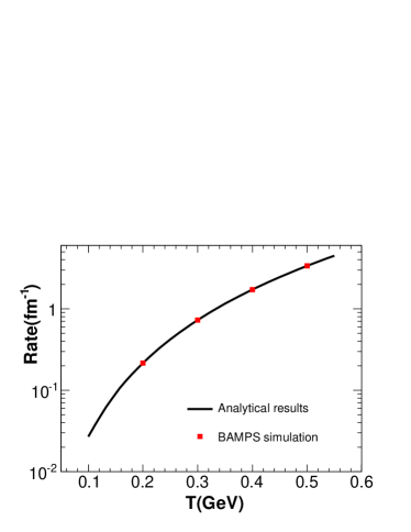
Figure 1: Collision rates per particle as a function of temperature. The solid squares show the numerically calculated collision rates with $N_{test}=1600$, while the solid curve depicts the analytical results.

For the first test we assume an equilibrium initial condition obeying the Bose-Einstein distribution, i.e., $\mu=0$ in Eq. (1). We compare the collision rate per particle obtained from the numerical calculations with the analytical results by integrating Eq. (3) over the full phase space. Figure 1 shows the comparisons for various temperatures. The squares denote the numerical results and the solid curve depicts the analytical rates. We see a very good agreement between the numerical and analytical collision rates.

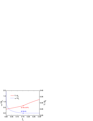
Figure 2: Dependence of the chemical potential $\mu$ and the temperature $T$ on $f_{0}$ and $Q_{s}$.

As the next we prove the equilibration of bosons with an out of equilibrium initial distribution,

$$f_{init}({\mathbf{p}})=f_{0}\theta(Q_{s}-|{\mathbf{p}}|)\,,$$ (10)

which resembles that in the early stage of ultrarelativistic heavy ion collisions Blaizot:2011xf . $f_{0}$ and $Q_{s}$ are parameters, which simply model the relation to the colliding energy. The higher the colliding energy, the larger are $f_{0}$ and $Q_{s}$, and thus the larger are the particle number and energy density, which can be obtained from Eq. (10)

$$n_{init}=gf_{0}\frac{Q_{s}^{3}}{6\pi^{2}}\,,\ \ e_{init}=gf_{0}\frac{Q_{s}^{4}}{8\pi^{2}}\,,$$ (11)

where $g=1$ in this section. The initial momentum distribution has been simplified to be isotropic, although the new method introduced above can be applied for anisotropic momentum distributions.

For calculations in a box the energy density $e$ is conserved. Assuming binary collisions of particles only, the particle number density $n$ is also conserved during the equilibration. In particular, $n$ and $e$ are equal to those at equilibrium with the distribution function (1). Therefore, for given $f_{0}$ and $Q_{s}$ from the initial condition, the temperature $T$ and the chemical potential $\mu$ at equilibrium can be calculated. In Fig. 2 we plot $T/Q_{s}$ and $-\mu/Q_{s}$ as functions of $f_{0}$. The kinks at $f_{0}^{c}=0.154$ indicate a transition from normal gluon gas to the one with the appearance of a BEC, since $\mu$ must keep zero for increasing $f_{0}$ (or density).

For $f_{0}>f^{c}_{0}$ the particle system is initially over-populated and a BEC will occur during the equilibration. At thermal equilibrium the distribution function contains the Bose-Einstein distribution and a condensate,

$$f_{eq}({\mathbf{p}})=\frac{1}{e^{E/T}-1}+(2\pi)^{3}n_{c}^{eq}\delta^{(3)}({\mathbf{p}})\,,$$ (12)

where $n_{c}^{eq}$ is the density of the condensate particles. From the particle number and energy conservation we obtain easily that

$$T = \left(\frac{15f_{0}}{4}\right)^{1/4}\frac{Q_{s}}{\pi}\,,$$ (13)

$$n_{c}^{eq} = n_{init}\left[1-\zeta(3)\frac{6}{\pi^{3}}\left(\frac{15}{4}\right)^{3/4}\left(\frac{1}{f_{0}}\right)^{1/4}\right]\,.$$ (14)

From the above equation we can also obtain $f_{0}^{c}$, at which $n_{c}^{eq}=0$. We see that $f_{0}^{c}$ is independent of $Q_{s}$.

For $f_{0}<f_{0}^{c}$ the system is under-populated. In this section we present thermalization of systems with $Q_{s}=1\mbox{ GeV}$ and two sets of $f_{0}$, $f_{0}=0.05$ and $f_{0}=f_{0}^{c}$. In both cases no BEC will appear. The difference from one to another case is that for $f_{0}=0.05$ the equilibrium momentum distribution $f_{eq}$ converges to $1/(e^{-\mu/T}-1)$ at $p\to 0$, while for $f_{0}=f_{0}^{c}$ it diverges at $p\to 0$.

For $f_{0}=0.05$ the time evolution of the particle momentum distribution is shown in Fig. 3.

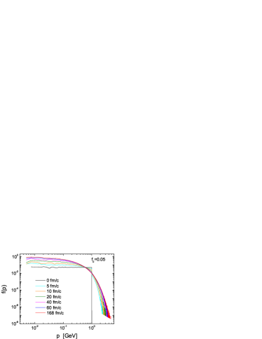
Figure 3: The time evolution of the momentum distribution function for $f_{0}=0.05$.

$f$ is calculated at a set of equidistant momenta with $\Delta p=2.5\mbox{ MeV}$, beginning from $5\mbox{ MeV}$. We find a gradual equilibration with a large timescale of about $170\mbox{ fm/c}$. During the equilibration particles, which mainly populate at $Q_{s}$ in the initial condition, flow into the lower and higher momentum region. We see that the statistical fluctuation is strong at very low and very high momentum region due to small particle populations. One needs large value of $N_{test}$ to reduce these fluctuations. In this calculation $N_{test}=691000$ is used.

From the calculations, which results are presented in Fig. 2, we obtain $T=0.258\mbox{ GeV}$ and $\mu=-0.205\mbox{ GeV}$ for $f_{0}=0.05$. In Fig. 4 we compare the momentum distribution at $168\mbox{ fm/c}$ with the thermal equilibrium distribution (1).

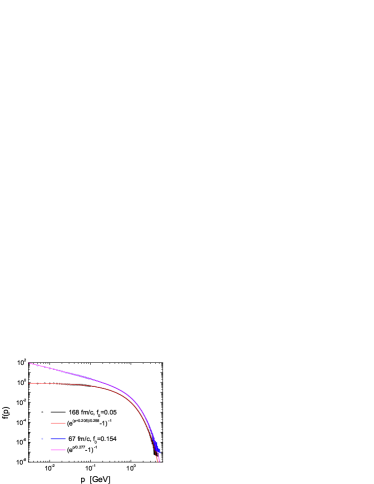
Figure 4: Comparisons between the calculated distributions at equilibrium times and the Bose-Einstein distributions with the expected temperatures and chemical potentials.

The open circles depict the first $40$ values of the calculated distribution separated by a equidistant interval of $\Delta p=2.5\mbox{ MeV}$ and beginning with $5\mbox{ MeV}$. We see a perfect agreement over $7$ orders in magnitude.

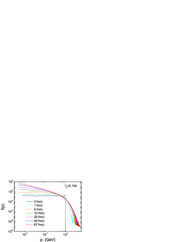
Figure 5: Same as Fig. 3, but for $f_{0}=0.154$.

The equilibration for $f_{0}=f_{0}^{c}$ is presented in Fig. 5. In this calculation $N_{test}=230000$ is used. We see the divergence of $f(p)$ at $p\to 0$. The equilibration has a shorter timescale of about $65\mbox{ fm/c}$ due to a larger density, compared with that for $f_{0}=0.05$. Also, the calculated momentum distribution at $67\mbox{ fm/c}$ agrees well with the Bose-Einstein distribution with $T=0.277\mbox{ GeV}$ and $\mu=0$, as seen in Fig. 4.

The perfect agreements between the numerical results and analytical solutions shown in this section demonstrate the correct implementation of the new method solving the Boltzmann equation with Bose statistics.

III The onset of Bose-Einstein condensation

After we have proven the numerical implementation for collisions of bosons in the previous section, we consider in the rest of the paper an over-populated system of massless gluons. For this we set $Q_{s}=1\mbox{ GeV}$ and $f_{0}=1$ in the initial distribution (10). For the BAMPS calculation $N_{test}=2400$ is used. Although $N_{test}$ is smaller than those used for $f_{0}=0.05$ and $f_{0}=0.154$ in the previous section, the total number of test particles is almost the same, because gluons have a degeneracy factor of $g=16$. In this section we study the onset of Bose-Einstein condensation. In the next section we demonstrate the full thermalization of gluons with a complete Bose-Einstein condensation.

The elastic scatterings of massless gluons are described in leading order of perturbative QCD. We use the same matrix element as that in our previous work Xu:2014ega ,

$$|{\cal M}_{gg\to gg}|^{2}\approx 144\pi^{2}\alpha_{s}^{2}\frac{s^{2}}{t(t-m^{2}_{D})}\,,$$ (15)

which is calculated by using the Hard-Thermal-Loop (HTL) treatment Aurenche:2002pd ; Kurkela:2011ti . $s$ and $t$ are the Mandelstam variables, and $m_{D}$ is the screening mass

$$m^{2}_{D}=16\pi N_{c}\alpha_{s}\int\frac{d^{3}p}{(2\pi)^{3}}\,\frac{1}{p}f\,.$$ (16)

The matrix element obeys the general condition for the occurrence of Bose-Einstein condensation. This will become clear in the next section, when we describe the condensation of gluons. The coupling is set to be $\alpha_{s}=0.3$ throughout the paper.

According to the definition (4) we obtain the total cross section

$$\sigma_{gg\to gg}=\frac{9}{2}\pi\frac{\alpha_{s}^{2}}{m_{D}^{2}}\ln\frac{1-m_{D}^{2}/t_{cut}}{1+m_{D}^{2}/s}\,,$$ (17)

where the logarithmic divergence has been regularized by an upper cutoff of $t$, $t_{cut}$. $t_{cut}$ is determined in consistency with the cross section of collisions involving condensate particles, which will be clarified in the next section. We note that scatterings with $t$ approaching to zero do not contribute to thermalization.

Figure 6 shows the time evolution of the distribution function.

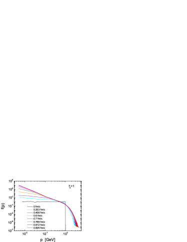
Figure 6: Same as Fig. 3, but for $f_{0}=1$.

At the first sight we see a transportation of particles as well as energies from $Q_{s}=1\mbox{ GeV}$ towards regions of lower and higher momentum. More elaborate analyses carried out below will expose finer structures of $f(p)$.

Theoretical studies Semikoz:1994zp showed that the kinetic Boltzmann equation (II) has temporally self-similar solutions. In a quasi-stationary state $f(p)$ is a scaling invariant power law function $f(p)\sim p^{-r}$ at momentum $p$, where $f(p)\gg 1$. The exponent $r$ depends on the scaling behavior of the matrix element under rescaling of the momentum. For our case (15) we follow the derivations in Ref. Semikoz:1994zp ; Meistrenko:2015mda and obtain $r=2$ in a turbulent state with constant transport of particle number (called as particle cascade), and $r=7/3$ in a turbulent state with constant energy transport (called as energy cascade).

We show $p^{2}f(p)$ at four various times in Fig. 7.

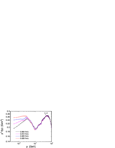
Figure 7: The particle distribution function multiplied by momentum squared.

The symbols depict the extracted values of $f$ at first $12$ momenta. If there exists a particle cascade [$f(p)\sim p^{-2}$], we will see a plateau of $p^{2}f(p)$ within a momentum interval. This is indeed seen from the time $0.812$ fm/c to $0.826$ fm/c from $p\approx 0.03\mbox{ GeV}$ towards the infrared region. We note that the extraction of $f(p)$ at $p<5\mbox{ MeV}$ is inaccurate, because the number of test particles at the deep infrared region in the present calculation is too small to overcome statistical fluctuations. Thus, we end the calculation, when $f(p)$ at $p>5\mbox{ MeV}$ reaches the scaling behavior $f(p)\sim p^{-2}$. With a much larger $N_{test}$ in future calculations we could obtain more accurate values of $f(p)$ in the deep infrared region.

In Fig. 7 we see that the height of the plateau increases with time, which indicates that $f(p)$ at the plateau is time dependent and not stationary. The reason is due to two other power law scalings at higher momentum. The second power law scaling is between $p\approx 0.03\mbox{ GeV}$ and $0.1\mbox{ GeV}$, where the exponent is larger than $2$, and the next is between $0.1\mbox{ GeV}$ and $0.5\mbox{ GeV}$, where the exponent is smaller than $2$. Both exponents can be extracted through fitting $f(p)$ by using power law functions. We find that the exponent of the second scaling is $7/3$, which corresponds to the energy cascade and is better seen in Fig. 8, where $p^{7/3}f(p)$ is plotted.

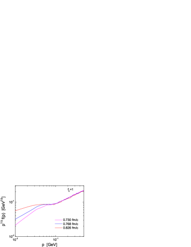
Figure 8: The particle distribution function multiplied by momentum to a power of $7/3$.

The plateau appears at $p\approx 0.1\mbox{ GeV}$ at $0.73$ fm/c and extends towards lower momentum with increasing time. The $p^{-7/3}$ scaling appears earlier than the $p^{-2}$ scaling that appears at about $0.81$ fm/c. We also see that the height of the plateau in $p^{7/3}f(p)$, on the contrary to that in $p^{2}f(p)$, does not change, which indicates that the plateau in $p^{7/3}f(p)$ is the region of the stationary turbulence. Since the $p^{-2}$ scaling region of $f(p)$ connects the lower momentum end of the $p^{-7/3}$ scaling region, the extending $p^{-7/3}$ scaling region towards lower momentum causes the increase of $f(p)$ in the $p^{-2}$ scaling region, as already observed in Fig. 7.

The stationary turbulence region with $f(p)\sim p^{-7/3}$ is followed by a further power law scaling with $f(p)\sim p^{-7/4}$, as shown in Fig. 9, where $p^{7/4}f(p)$ is plotted.

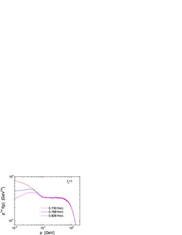
Figure 9: The particle distribution function multiplied by momentum to a power of $7/4$.

This power law scaling is not known so far in the literature. Even not obviously, we can recognize that in the new power law scaling region $f(p)$ is not stationary. The height of the plateau in Fig. 9 decreases slightly with increasing time. Roughly speaking, particles and energies in the $p^{-7/4}$ scaling region transport through the stationary $p^{-7/3}$ scaling region towards lower momentum region, where the $p^{-2}$ scaling region extends to infrared momentum. At the same time it exits another particle and energy transport from the $p^{-7/4}$ scaling region towards higher momentum, which is, however, hardly seen in Fig. 6. The observed transportations are due to the initial condition given in this study, where most particles and energies are initialized at $p=Q_{s}=1\mbox{ GeV}$.

We note that it is surprising that we see both $p^{-2}$ and $p^{-7/3}$ scalings in our calculation, although the theoretical derivations of the two power law scalings are done with approximations. More calculations are required for the time evolution of $f(p)$ in the infrared momentum region and will be done in the future.

Even if future calculations could confirm the $p^{-2}$ power law scaling in the deep infrared region, this cannot lead to the formation of a BEC. To show this, we calculate the particle density at $p=0$ by integrating $f(p)$ over a sphere of radius $p_{0}$ and then going to the limit $p_{0}\to 0$,

$$n(p=0)=\lim_{p_{0}\to 0}\int_{0}^{p_{0}}\frac{dp}{2\pi^{2}}p^{2}f(p)\,.$$ (18)

For $f(p)\sim p^{-2}$ at low momentum, the particle density at $p=0$ vanishes. The study on the mechanism of a BEC formation is beyond the scope of this paper. We assume the formation of a small piece of BEC instantaneously at some timescale. The growth of the BEC can then be described by the kinetic Boltzmann equation, which we will present in the next section.

Since the mechanism of the Bose-Einstein condensation of gluons is not known yet, it is impossible to determine the exact time when the condensation begins. Nevertheless, one can make estimates on this timescale by looking at the possible onset of the gluon condensation. In our previous work Xu:2014ega we have fitted the gluon distribution at low momenta by the Bose-Einstein distribution with an effective temperature and an effective chemical potential. The latter increases from a negative value to zero, which is assumed to be reached at the onset of the gluon condensation. Thus, we have chosen the moment as the start time of the gluon condensation, $t_{c}$, once the effective chemical potential becomes positive due to the numerical fluctuation around zero. Thus, at $t_{c}$ the distribution function at low momenta has a $1/p$ power law form. In this section we have found that the distribution function at low momenta evolves further from $1/p$ to $1/p^{2}$. The latter behavior is expected as a fix point corresponding to a constant particle transportation. Due to the new observation we choose $t_{c}$, different from that in the previous work, as the time when the $1/p^{2}$ power law distribution is achieved at low momenta ($\sim 5\mbox{ MeV}$). The calculation shows that $t_{c}=0.826\mbox{ fm/c}$.

IV Bose-Einstein condensation

In this section we continue the calculate in the previous section and study the time evolution of the particle distribution function $f(p,t)$ in the presence of a BEC. $f(p,t)$ is decomposed into two parts $f=f^{g}+f^{c}$, where $f^{g}$ denotes the distribution of gas (noncondensate) particles and $f^{c}=(2\pi)^{3}n_{c}\delta^{(3)}({\mathbf{p}})$ denotes the distribution of the condensate particles with zero momentum. Same as for the onset of the condensation, we consider here elastic collisions only. Denoting gas particles by $g$ and condensate particles by $c$, we consider $g+g\to g+g$, $g+c\to g+g$, and $g+g\to g+c$ processes. The Boltzmann equations for gas and condensate particles are then given as follows:

$$\frac{\partial f^{g}_{1}}{\partial t}=\frac{1}{2E_{1}}\int d\Gamma_{2}\frac{1}{2}\int d\Gamma_{3}d\Gamma_{4}|{\cal M}_{34\to 12}|^{2}$$

$$\times\ \left[f^{g}_{3}f^{g}_{4}(1+f^{g}_{1})(1+f^{g}_{2})+f^{g}_{3}f^{g}_{4}(1+f^{g}_{1})f^{c}_{2}\right.$$

$$\ \ \ \ +f^{c}_{3}f^{g}_{4}(1+f^{g}_{1})(1+f^{g}_{2})+f^{g}_{3}f^{c}_{4}(1+f^{g}_{1})(1+f^{g}_{2})$$

$$\ \ \ \ -f^{g}_{1}f^{g}_{2}(1+f^{g}_{3})(1+f^{g}_{4})-f^{g}_{1}f^{c}_{2}(1+f^{g}_{3})(1+f^{g}_{4})$$

$$\ \ \ \,\left.-f^{g}_{1}f^{g}_{2}f^{c}_{3}(1+f^{g}_{4})-f^{g}_{1}f^{g}_{2}(1+f^{g}_{3})f^{c}_{4}\right]$$

$$\times(2\pi)^{4}\delta^{(4)}(p_{3}+p_{4}-p_{1}-p_{2})\,,$$ (19)

$$\frac{\partial f^{c}_{1}}{\partial t}=\frac{1}{2E_{1}}\int d\Gamma_{2}\frac{1}{2}\int d\Gamma_{3}d\Gamma_{4}|{\cal M}_{34\to 12}|^{2}$$

$$\times\ \left[f^{g}_{3}f^{g}_{4}f^{c}_{1}(1+f^{g}_{2})-f^{c}_{1}f^{g}_{2}(1+f^{g}_{3})(1+f^{g}_{4})\right]$$

$$\times(2\pi)^{4}\delta^{(4)}(p_{3}+p_{4}-p_{1}-p_{2})\,.$$ (20)

The terms of the spatial derivative of $f^{g}_{1}$ and $f^{c}_{1}$ drop out, since we restrict ourselves to consider a spatially homogeneous gluon matter.

Before we come to the numerical implementations for solving the Boltzmann equations (IV) and (IV), we first show that the matrix element (15) describes the condensation process with a finite rate. For this purpose we integrate Eq. (IV) over ${\mathbf{p}}_{1}$, which gives the time derivative of the density of condensate particles. After a lengthy calculation for the integral of the right-hand side of Eq. (IV), which details are given in Appendix A, we obtain

$$\frac{\partial n_{c}}{\partial t}=\frac{n_{c}}{64\pi^{3}} \int dE_{3}dE_{4}\left[f_{3}^{g}f_{4}^{g}-f_{2}^{g}(1+f_{3}^{g}+f_{4}^{g})\right]$$ (21)

$$\times\ E\left[\frac{|{\cal M}_{34\to 12}|^{2}}{s}\right]_{s=2mE}\,.$$

The two terms on the right-hand side of Eq. (21) correspond to kinetic processes for the condensation and the evaporation, respectively. $E=E_{3}+E_{4}$ is the total energy in the collision, $p=|{\mathbf{p}}_{3}+{\mathbf{p}}_{4}|$ is the total momentum, and $s=E^{2}-p^{2}$ is the invariant mass. $m$ denotes the particle mass at rest, which is zero for gluons. From Eq. (21) we see that in order to describe the gluon condensation with a finite rate, the ratio $|{\cal M}_{34\to 12}|^{2}/s$ at $s=0$ should be nonzero and finite. This is fulfilled for the matrix element (15), since

$$\left[\frac{|{\cal M}_{34\to 12}|^{2}}{s}\right]_{s=0} = 144\pi^{2}\alpha_{s}^{2}\left[\frac{s}{t(t-m^{2}_{D})}\right]_{s=0}$$ (22)

$$= 144\pi^{2}\alpha_{s}^{2}\frac{1}{m^{2}_{D}}$$

is nonzero and finite. For the constant cross section with the isotropic distribution of collision angles the corresponding matrix element is proportional to $s$. Therefore, in this case, the condensation process of gluons has a finite rate too.

In the following we show how we solve Eqs. (IV) and (IV) numerically. We note that the numerical implementations are general and do not require in particular the isotropy of the momentum, which is needed to derive Eq. (21). Since we have assumed the isotropy of the momentum for simplicity, Eq. (21) is automatically solved by solving Eq. (IV). From Eq. (21) we see that the growth of the condensate needs an initial density, $n_{c}(t_{c})$. We take the density of such gluons, which energy is smaller than $5\mbox{ MeV}$, as $n_{c}(t_{c})$. This numerical handling will become clear later in this section.

Now we present the numerical method simulating collisions. For $g+g\to g+c$, which produces a condensate gluon, the integral in the effective cross section, Eq. (5), can be carried out analytically with help of delta-functions in $f^{c}_{1}\sim n_{c}\delta^{(3)}({\mathbf{p}_{1}})$ and for energy-momentum conservation. That is

$$\sigma_{c}^{eff} = \frac{1}{2s}\int d\Gamma_{1}d\Gamma_{2}|{\cal M}_{34\to 12}|^{2}f^{c}_{1}(1+f^{g}_{2})$$ (23)

$$\times(2\pi)^{4}\delta^{(4)}(p_{3}+p_{4}-p_{1}-p_{2})$$

$$= \frac{1}{2}\left[\frac{|{\cal M}_{34\to 12}|^{2}}{s}\right]_{s=0}\int d\Gamma_{1}d\Gamma_{2}f^{c}_{1}(1+f^{g}_{2})$$

$$\times(2\pi)^{4}\delta^{(4)}(p_{3}+p_{4}-p_{1}-p_{2})$$

$$= \pi n_{c}\left[\frac{|{\cal M}_{34\to 12}|^{2}}{s}\right]_{s=0}\frac{1}{2p}[1+f^{g}(p)]$$

$$\times\delta[(E-p)^{2}]\,.$$

Compared with Eq. (5), the factor $1/2$ drops out, because we fix particle $1$ to be the condensate gluon. The details of the integration can be found in Appendix B.

In principle, one can compute the collision probability $P_{g+g\to g+c}$ by putting Eq. (23) into Eq. (7). However, due to the divergence indicated by the delta-function in $\sigma_{c}^{eff}$, $P_{g+g\to g+c}$ is not computable. The divergence of $\sigma_{c}^{eff}$ corresponds to $s=0$, in which case the momenta of the two incoming gluons are parallel. In other words, only if $s=0$, a condensate gluon can be produced in a $g+g\to g+c$ process. The probability for this process is infinity. The two extreme values, zero phase space and infinite collision probability, give nevertheless a finite collision rate, as indicated in Eq. (21). However, in numerical calculations, it is almost impossible to find two particles with parallel momentum. Moreover, it is also impossible to deal with processes with infinite collision probability. To overcome this difficulty we have to make an approximation. We define an energy cutoff $\varepsilon$. Gluons with energy smaller than $\varepsilon$ are regarded as condensate gluons. This approximation, which has the same mean as the regularization by a nonzero but small effective gluon mass, breaks the rule that momenta of two incoming gluons in a $g+g\to g+c$ process should be parallel, or, $s=0$. A $g+g\to g+c$ process is now allowed to occur with a nonzero but small angle $\alpha_{c}$ between the momenta of two incoming gluons, or, with a nonzero but small $s$. Accordingly the divergence in $\sigma_{c}^{eff}$ is eliminated, although $\sigma_{c}^{eff}$ is still large. The smaller the value of $\varepsilon$, the smaller is $\alpha_{c}$ and the larger is $\sigma_{c}^{eff}$. Mathematically, the approximation leads to the replacement of the delta-function in $f^{c}_{1}$ by a step function,

$$\delta^{(3)}({\mathbf{p}_{1}})\approx\frac{\theta(\varepsilon-p_{1})}{4\pi p_{1}^{2}\varepsilon}\,.$$ (24)

Putting Eq. (24) into Eq. (23) we obtain

$$\sigma_{c}^{eff} = \pi n_{c}\left[\frac{|{\cal M}_{34\to 12}|^{2}}{s}\right]_{s=0}\frac{1}{2p}[1+f^{g}(p)]$$ (25)

$$\times\frac{1}{4\varepsilon}\left(\frac{2}{E-p}-\frac{1}{\Delta}\right)\theta\left(\varepsilon-\frac{E-p}{2}\right)\,,$$

where $\Delta=\min\{\varepsilon,(E+p)/2\}$. In Appendix B one can find more detailed calculations. Since $s=E^{2}-p^{2}$, the step function in $\sigma_{c}^{eff}$ leads to the maximum of $s$, $s_{m}=2\varepsilon(E+p)$, below which a $g+g\to g+c$ can occur. In addition, $s_{m}$ corresponds to the maximal angle between the momenta of two incoming gluons.

In the previous section we have presented the numerical implementation of $g+g\to g+g$ processes in absence of the gluon condensate. Numerically we turn off $g+g\to g+c$ processes by setting $\sigma_{c}^{eff}=0$. On the other hand, with the cross section (17), collisions can still occur at $s<s_{m}$, and gluons with energy being less than $\varepsilon$ can still be produced. Therefore, at the time $t_{c}$ when we turn on $g+g\to g+c$ processes to describe the condensation, we will have a nonzero density of condensate particles. This density $n_{c}$ at $t_{c}$, which is needed to solve Eq. (IV), is not physically motivated, but regarded as an initial seed for the growth of the condensate. The smaller the value of $\varepsilon$, the smaller is $n_{c}(t_{c})$. This will not lead to significant difference in the increase of $n_{c}$, provided that $n_{c}(t_{c})$ is much smaller than its final equilibrium value, which is true in our case.

With the approximated $\sigma_{c}^{eff}$ we compute the collision probability $P_{g+g\to g+c}$ according to Eq. (7) and simulate the $g+g\to g+c$ process. The effect on the collision rate due to the approximation with the energy cutoff is negligible, if $\varepsilon$ is small enough. In the present calculation we set $\varepsilon=2.5\mbox{ MeV}$, which corresponds to the limitation that the extraction of $f$ below $5\mbox{ MeV}$ is inaccurate due to small numbers of test particles. In Appendix C we show the potential moderate effect on the collision rate, if $\varepsilon$ becomes large.

The numerical implementation for back reactions $c+g\to g+g$ is same as that for $g+g\to g+g$, which has been presented in the previous section. Compared with $\sigma_{g+g\to g+g}$ (17), the total cross section for $c+g\to g+g$ is

$$\sigma_{c} = \frac{1}{2}\int_{-s}^{0}dt\frac{|{\cal M}_{34\to 12}|^{2}}{16\pi s^{2}}$$ (26)

$$= \frac{1}{32\pi s}\int_{-s}^{0}dt\left[\frac{|{\cal M}_{34\to 12}|^{2}}{s}\right]_{s=0}$$

$$= \frac{1}{32\pi s}\int_{-s}^{0}dt144\pi^{2}\alpha_{s}^{2}\frac{1}{m^{2}_{D}}=\frac{9}{2}\pi\frac{\alpha_{s}^{2}}{m_{D}^{2}}\,.$$

Due to the kinematic reason it is always true that $s\leq s_{m}$ in each $c+g\to g+g$ process. Numerically, if $s\leq s_{m}$ we use $\sigma_{c}$, if $s>s_{m}$ we use $\sigma_{g+g\to g+g}$ (17). We assume a continuous change of the cross section with respect to $s$. Thus, $\sigma_{g+g\to g+g}$ should be equal to $\sigma_{c}$ at $s_{m}$. With this condition we determine $t_{cut}$ in Eq. (17), which is $t_{cut}=-m_{D}^{2}/[e(1+m_{D}^{2}/s_{m})-1]$.

From Eq. (IV) we recognize that both the collision rate of $g+g\to g+c$ and that of $c+g\to g+g$ contain a same contribution, which is proportional to $f_{4}^{g}f_{3}^{g}f_{2}^{g}f_{1}^{c}$. Therefore, the term being proportional to $f^{g}(p)=f_{2}^{g}$ in Eq. (25) corresponds to this contribution in $g+g\to g+c$ processes ($4+3\to 2+1$), while the term being proportional to $f_{3}^{g}f_{4}^{g}$ in $P^{\prime}_{22}$ [see Eq. (9)] corresponds to the same contribution in $c+g\to g+g$ ($1+2\to 3+4$) processes. The two contributions cancel out. In numerical calculations we thus replace $1+f^{g}(p)$ in Eq. (25) by $1$ and replace the Bose factor $(1+f_{3}^{g})(1+f_{4}^{g})$ in $P^{\prime}_{22}$ by $1+f^{g}_{3}+f^{g}_{4}$. More details can be found in Appendixes A and B.

In Fig. 10 we show the time evolution of the momentum distribution of gluons from $t_{c}$, when the condensation begins, to a later time $6.692\mbox{ fm/c}$, when the condensation is complete.

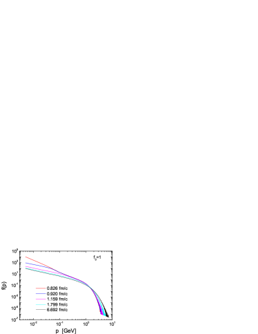
Figure 10: Same as Fig. 6.

With the growing gluon condensate we find a rapid change of the distribution at low momentum from the $p^{-2}$ scaling at $t_{c}=0.826\mbox{ fm/c}$ to $p^{-1}$ at $0.92\mbox{ fm/c}$. During this time the $p^{-7/3}$ scaling remains. As the time further proceeds, the $p^{-1}$ scaling extends to larger momentum region, so that the region with the $p^{-7/3}$ scaling completely disappears at $1.159\mbox{ fm/c}$. Due to the growth of the condensate the particle distribution at low momentum decreases. The energies freed from condensation are transferred to particles with larger momentum because of the energy conservation. This energy transfer leads to the increase of the distribution function at large momentum. Figure 11 shows the comparison of the gluon distribution at $6.692\mbox{ fm/c}$ with the Bose-Einstein distribution function with $T=0.443\mbox{ GeV}$ and $\mu_{eq}=0$.

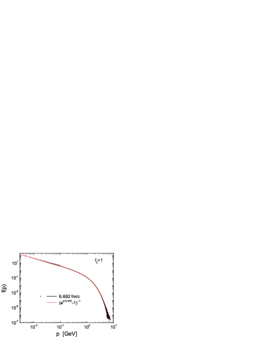
Figure 11: Comparison of the gluon momentum distribution at $6.692\mbox{ fm/c}$ (black open circles and solid curve) with the Bose-Einstein distribution at thermal equilibrium (red curve).

The latter is the thermal equilibrium distribution when the condensation is complete, see Eq. (13). The open circles depict the first $40$ values of the calculated distribution separated by a equidistant interval of $\Delta p=2.5\mbox{ MeV}$ and beginning from $5\mbox{ MeV}$. We see that the calculated result agrees nicely with the analytical distribution over $8$ orders in magnitude. Particularly we see agreements at very low as well as very high momentum, where strong statistical fluctuations are expected due to small particle numbers.

We show in Fig. 12 the growth of the gluon condensate in time, divided by the expected density at equilibrium, given in Eq. (14).

Figure 12: Time evolution of the density of the gluon condensate.

Before the condensation really starts at $t_{c}=0.826\mbox{ fm/c}$, the meaning of $n_{c}$ is the density of gluons, which energy is smaller than $2.5\mbox{ MeV}$. The increase of this density is due to collisions of gluons without the presence of a gluon condensate. We see that the increase of this density is almost exponential. At $t_{c}$ the density reaches about $1\%$ of the value of the condensate density at equilibrium. This value is regarded as a seed for the growth of the condensate.

Once the condensation starts, $n_{c}$ denotes the density of the condensate, although $n_{c}$ is still calculated as the density of gluons with energy being smaller than $2.5\mbox{ MeV}$ due to the numerical handling explained before in this section. In the upper panel of Fig. 12 we see a much stronger increase of $n_{c}$ after $t_{c}$ than that before $t_{c}$. At early times of the condensation the production processes are dominant compared to the evaporation processes. At these times the gluon condensate grows exponentially, which can qualitatively be understood by Eq. (21). When the evaporation processes begin to balance the production processes, the growth of the gluon condensate slows down, and $n_{c}$ relaxes to its final value at thermal equilibrium. The relaxation of the calculated $n_{c}$ to the expected value at equilibrium (see the lower panel of Fig. 12) and the agreement of the distribution of non-condensate gluons with the expected Bose-Einstein function (see Fig. 11) demonstrate the correct numerical implementations for solving the Boltzmann equation with the presence of a Bose-Einstein condensate.

During the thermalization the typical hard momentum, which is $Q_{s}$ initially, increases, as the energy flows towards the ultraviolet momentum region. As suggested in Ref. Berges:2013fga , we define the hard momentum scale $\Lambda(t)$ as

$$\Lambda^{2}(t)=\frac{\int d\Gamma 4p^{2}Ef^{g}({\mathbf{p}},t)}{\int d\Gamma Ef^{g}({\mathbf{p}},t)}\,.$$ (27)

If the solution of the Boltzmann equation (IV) is self-similar, i.e., $f^{g}({\mathbf{p}},t)=t^{\alpha}f_{s}(t^{\beta}{\mathbf{p}})$, then the hard scale shows a scaling behavior Berges:2013fga , $\Lambda(t)\sim t^{-\beta}$. Following the derivation in Micha:2004bv ; Berges:2013fga , the exponents $\alpha$ and $\beta$ can be obtained by putting the self-similar solution into Eq. (IV) and using the energy conservation. The values of the exponents depend on the matrix element. For our case [see Eq. (15)] we obtain $\alpha=-4/5$ and $\beta=-1/5$. Figure 13 shows the time evolution of the hard scale $\Lambda(t)$ compared with a function $\sim t^{-1/5}$.

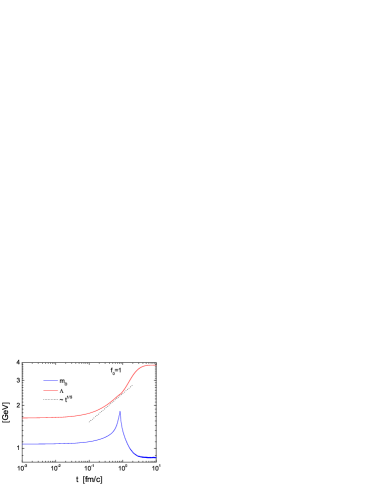
Figure 13: Time evolution of the hard scale $\Lambda$ and the Debye screening mass $m_{D}$.

We see the agreement in a time window between $0.3\mbox{ fm/c}$ and $t_{c}=0.826\mbox{ fm/c}$. This indicates that within this time window a self-similar distribution is achieved over a momentum region, which is sensitive to the hard scale. After $t_{c}$ the condensation occurs, which accelerates the energy transportation towards the ultraviolet momentum region. The increase of $\Lambda(t)$ becomes stronger. As the condensation completes, $\Lambda(t)$ relaxes to its value at equilibrium, which is $4\pi\sqrt{10/21}T$.

In Fig. 13 we also show the time evolution of the Debye screening mass $m_{D}$, which squared is defined in Eq. (16) with $f^{g}$ instead of $f$. $m_{D}(t)$ is governed by low momenta. Before $t_{c}$ the over-population of the low momentum gluons leads to a rapid increase of $m_{D}$ to infinity. The Bose-Einstein condensation after $t_{c}$ reduces the over-population, which then leads to the decrease of $m_{D}$. At thermal equilibrium $m_{D}$ relaxes to $\sqrt{4\pi\alpha_{s}}T$. Both relaxation values of $\Lambda$ and $m_{D}$ from the calculation agree well with the expected equilibrium values.

V Summary

In this paper we have presented a new numerical method, which solves Boltzmann equations for bosons, in particular, with the presence of a Bose-Einstein condensate. Compared to the old method, which has been developed in BAMPS to describe collisions of Boltzmann particles, the new method takes Bose statistics into account by considering the angular differential collision probability instead of the total collision probability, which is more time consuming in practice. Moreover, the new method does not require any approximations to matrix elements of interactions and, thus, is a general scheme. The numerical implementation of this new method has been well tested by performing box calculations for static particle systems. First we have considered systems at thermal equilibrium with the Bose-Einstein distribution at various temperatures and calculated the collision rate. We have seen that the calculated collision rates agree well with the expected analytical values. Second, we have assumed two different non-thermal initial conditions and evolved systems to the equilibrium states. The expected equilibrium distributions are Bose-Einstein functions with negative and zero chemical potentials. We have found that in both cases the final distributions from the calculations agree well with the expected analytical functions. These successes demonstrate the correct implementations of Bose statistics in the Boltzmann equation for bosons through the new method.

Employing the tested numerical implementations we have then investigated the onset of the Bose-Einstein condensation for an initially over-populated gluon system, before the Bose-Einstein condensation occurs. Due to the Bose statistical factor the distribution at low momenta increases quickly to be over-populated and is thus far from thermal equilibrium. By looking at the time evolution of the momentum distribution function we have observed the appearance of two power law scalings, $p^{-2}$ in the infrared and $p^{-7/3}$ in the intermediate momentum region. The two power law scaling functions have exactly the same exponents as those suggested by the scaling arguments for the solutions to the Boltzmann equation in momentum regions, where $f(p)\gg 1$. The $p^{-7/3}$ scaling function is self-similar within a small momentum window, which may be sensitive to the hard momentum scale, because the time evolution of the hard scale shows the expected power law scaling behavior before the onset of the Bose-Einstein condensation and thus reflects the self-similarity of the particle distribution. The $p^{-2}$ scaling is, however, not yet self-similar as suggested, because the $p^{-7/3}$ scaling extends to the infrared region, so that the magnitude of the $p^{-2}$ scaling function increases with time. This behavior leads to an energy transport towards $p=0$ besides a particle transport. Since the distribution function for $p<5\mbox{ MeV}$ cannot be calculated with the required accuracy due to the limitation of the current numerical computation, our calculation has to be stopped at some time, when the $p^{-2}$ scaling extends to the region of $p<5\mbox{ MeV}$. The answer to the question whether the $p^{-2}$ scaling will become self-similar at some later time has to be postponed to a future work. Besides the two scalings suggested we have also found a further power law scaling, $p^{-7/4}$, following the $p^{-7/3}$ scaling. The distribution function in this new scaling region is decreasing in time, which leads to the transportation of particles and energies through the $p^{-7/3}$ scaling region into the $p^{-2}$ scaling region.

Finally the Boltzmann equation is solved with the presence of a Bose-Einstein condensate. We have found that if the condensate consists of massless particles, the matrix element of interactions between condensate and non-condensate particles should be constrained by the requirement that the ratio of the matrix element squared to the invariant mass $s$ must be finite at $s\to 0$. The matrix element of gluon scatterings, which is motivated by the HTL calculations and has been already employed in the calculation for the onset of the gluon condensation, fulfills this constraint. We have continued the calculation for the onset with a seed for the growth of the condensate and demonstrated the gluon condensation from an out of equilibrium state. The condensation reduces the over-population of gluons at low momenta. The energy freed from the condensation is transferred to particles with large momentum. As the condensation becomes complete, the system of non-condensate gluons approaches thermal equilibrium, which agrees well with the expected Bose-Einstein distribution.

To know whether a gluon condensate exists and to further understand thermalization in heavy-ion collisions, we need more further investigations. As the next, we will study the role of inelastic scatterings Huang:2013lia ; Blaizot:2016iir and expansion in the possible formation of a gluon condensate.

Appendix A Rate equation of the condensation

In this section we derive the rate equation of the condensation, Eq. (21), from Eq. (IV). Integrating Eq. (IV) over the momentum of the condensate particle $d^{3}p_{1}/(2\pi)^{3}$ gives the time derivative of the density of condensate particles

$$\frac{\partial n_{c}}{\partial t} = \frac{1}{2}\int d\Gamma_{1}d\Gamma_{2}\int d\Gamma_{3}d\Gamma_{4}|{\cal M}_{34\to 12}|^{2}(2\pi)^{4}$$ (28)

$$\times\ \delta^{(4)}(p_{3}+p_{4}-p_{1}-p_{2})\left[f_{3}^{g}f_{4}^{g}f_{1}^{c}(1+f_{2}^{g})\right.$$

$$\left.-f_{1}^{c}f_{2}^{g}(1+f_{3}^{g})(1+f_{4}^{g})\right]$$

$$\equiv R_{c}^{gain}-R_{c}^{loss}\,,$$

where the first and second term are named as $R_{c}^{gain}$ and $R_{c}^{loss}$ denoting the condensation and evaporation rate, respectively.

In the following we carry out integrations in $R_{c}^{gain}$ explicitly. At first we integrate over $d^{3}p_{2}$ with help of the delta-function $\delta^{(3)}({\mathbf{p}}_{3}+{\mathbf{p}}_{4}-{\mathbf{p}}_{1}-{\mathbf{p}}_{2})$ and obtain

$$R_{c}^{gain} = \frac{1}{2}\int\frac{d^{3}p_{3}}{(2\pi)^{3}2E_{3}}\frac{d^{3}p_{4}}{(2\pi)^{3}2E_{4}}\frac{d^{3}p_{1}}{(2\pi)^{3}2E_{1}}\frac{1}{2(E-E_{1})}$$ (29)

$$\times\ |{\cal M}_{34\to 12}|^{2}2\pi\delta[F({\mathbf{p}}_{1})]f_{3}^{g}f_{4}^{g}f_{1}^{c}(1+f_{2}^{g})\,,$$

where $f_{2}^{g}=f^{g}(E-E_{1},{\mathbf{p}}-{\mathbf{p}}_{1};t)$, $E=E_{3}+E_{4}=E_{1}+E_{2}$ is the total energy and ${\mathbf{p}}={\mathbf{p}}_{3}+{\mathbf{p}}_{4}={\mathbf{p}}_{1}+{\mathbf{p}}_{2}$ is the total momentum. $\delta[F({\mathbf{p}}_{1})]$ indicates the energy conservation, where

$$F({\mathbf{p}}_{1}) = E-E_{1}-E_{2}=E-E_{1}-\sqrt{p^{2}_{2}+m^{2}}$$ (30)

$$= E-E_{1}-\sqrt{({\mathbf{p}}-{\mathbf{p}}_{1})^{2}+m^{2}}\,.$$

Using the identity

$$\int dE_{1}d^{3}p_{1}\delta(E_{1}^{2}-p_{1}^{2}-m^{2})=\int\frac{d^{3}p_{1}}{2E_{1}}$$ (31)

and $f_{1}^{c}=(2\pi)^{3}n_{c}\delta^{(3)}({\mathbf{p}}_{1})$ we then rewrite Eq. (29) to

$$R_{c}^{gain} = \pi n_{c}\int\frac{d^{3}p_{3}}{(2\pi)^{3}2E_{3}}\frac{d^{3}p_{4}}{(2\pi)^{3}2E_{4}}f_{3}^{g}f_{4}^{g}\int dE_{1}d^{3}p_{1}$$ (32)

$$\times\ \frac{1}{2(E-E_{1})}|{\cal M}_{34\to 12}|^{2}\delta(E_{1}^{2}-p_{1}^{2}-m^{2})\delta[F({\mathbf{p}}_{1})]$$

$$\times\ \delta^{(3)}({\mathbf{p}}_{1})(1+f_{2}^{g})\,.$$

As the next we integrate over $d^{3}p_{1}$ and then $dE_{1}$ using the delta function $\delta^{(3)}({\mathbf{p}}_{1})$ and $\delta[F({\mathbf{p}}_{1})]$

$$R_{c}^{gain} = \pi n_{c}\int\frac{d^{3}p_{3}}{(2\pi)^{3}2E_{3}}\frac{d^{3}p_{4}}{(2\pi)^{3}2E_{4}}f_{3}^{g}f_{4}^{g}\int dE_{1}\frac{1}{2(E-E_{1})}$$ (33)

$$\times\ |{\cal M}_{34\to 12}|^{2}\delta(E_{1}^{2}-m^{2})\delta(E-E_{1}-\sqrt{p^{2}+m^{2}})$$

$$\times\ (1+f_{2}^{g})$$

$$= \pi n_{c}\int\frac{d^{3}p_{3}}{(2\pi)^{3}2E_{3}}\frac{d^{3}p_{4}}{(2\pi)^{3}2E_{4}}f_{3}^{g}f_{4}^{g}\frac{1}{2\sqrt{p^{2}+m^{2}}}$$

$$\times\ |{\cal M}_{34\to 12}|^{2}\delta[(E-\sqrt{p^{2}+m^{2}})^{2}-m^{2}]$$

$$\times\ (1+f_{2}^{g})\,,$$

where $f_{2}^{g}=f^{g}(\sqrt{p^{2}+m^{2}},{\mathbf{p}};t)$. We denote that $\theta$ is the angle between ${\mathbf{p}}_{3}$ and ${\mathbf{p}}_{4}$. Then we have

$$p=|{\mathbf{p}}_{3}+{\mathbf{p}}_{4}|=\sqrt{p_{3}^{2}+p_{4}^{2}+2p_{3}p_{4}\cos\theta}\,.$$ (34)

We assume that the distribution function $f$ is isotropic in momentum space. Therefore, $f_{3}^{g}=f^{g}(p_{3},t)$, $f_{4}^{g}=f^{g}(p_{4},t)$, $f_{2}^{g}=f^{g}(p,t)$, and we can integrate Eq. (33) over the solid angles of ${\mathbf{p}}_{3}$ and ${\mathbf{p}}_{4}$

$$R_{c}^{gain} = \frac{n_{c}}{64\pi^{3}}\int dp_{3}dp_{4}\frac{p_{3}^{2}p_{4}^{2}}{E_{3}E_{4}}f_{3}^{g}f_{4}^{g}\int d\cos\theta\frac{1}{\sqrt{p^{2}+m^{2}}}$$ (35)

$$\times\ |{\cal M}_{34\to 12}|^{2}\delta[(E-\sqrt{p^{2}+m^{2}})^{2}-m^{2}]$$

$$\times\ (1+f_{2}^{g})\,.$$

The integral over $\cos\theta$ can be carried out using the delta funtion and gives

$$R_{c}^{gain} = \frac{n_{c}}{64\pi^{3}}\int dp_{3}dp_{4}\frac{p_{3}p_{4}}{E_{3}E_{4}}f_{3}^{g}f_{4}^{g}(1+f_{2}^{g})\frac{1}{2m}$$ (36)

$$\times\ \left[|{\cal M}|^{2}\right]_{E-\sqrt{p^{2}+m^{2}}=m}$$

$$= \frac{n_{c}}{64\pi^{3}}\int dE_{3}dE_{4}f_{3}^{g}f_{4}^{g}(1+f_{2}^{g})\frac{1}{2m}$$

$$\times\ \left[|{\cal M}|^{2}\right]_{E-\sqrt{p^{2}+m^{2}}=m}\,.$$

Since $s=E^{2}-p^{2}$, the constraint $E-\sqrt{p^{2}+m^{2}}=m$ is equivalent to $s=2mE$. This leads to

$$R_{c}^{gain}=\frac{n_{c}}{64\pi^{3}}\int dE_{3}dE_{4}f_{3}^{g}f_{4}^{g}(1+f_{2}^{g})E\left[\frac{|{\cal M}|^{2}}{s}\right]_{s=2mE}\,,$$ (37)

where $f_{2}^{g}=f^{g}(p,t)=f^{g}(\sqrt{E^{2}-2mE},t)$.

The integrals in $R_{c}^{loss}$ proceed similar as those shown above. We obtain $R_{c}^{loss}$ by replacing $f_{4}^{g}f_{3}^{g}(1+f_{2}^{g})$ in Eq. (37) with $f_{2}^{g}(1+f_{3}^{g})(1+f_{4}^{g})$. We have finally

$$\frac{\partial n_{c}}{\partial t} = \frac{n_{c}}{64\pi^{3}}\int dE_{3}dE_{4}[f_{3}^{g}f_{4}^{g}(1+f_{2}^{g})$$ (38)

$$\ \ \ \ \ \ \ \ \ -(1+f_{3}^{g})(1+f_{4}^{g})f_{2}^{g}]E\left[\frac{|{\cal M}|^{2}}{s}\right]_{s=2mE}$$

$$= \frac{n_{c}}{64\pi^{3}}\int dE_{3}dE_{4}[f_{3}^{g}f_{4}^{g}-f_{2}^{g}(1+f_{3}^{g}+f_{4}^{g})]$$

$$\ \ \ \ \ \ \ \ \ \times E\left[\frac{|{\cal M}|^{2}}{s}\right]_{s=2mE}\,,$$

which is Eq. (21). We see that both $R_{c}^{gain}$ and $R_{c}^{loss}$ contain a same contribution, which is proportional to $f_{4}^{g}f_{3}^{g}f_{2}^{g}$. The two contributions cancel out.

Appendix B The effective cross section for $g+g\to g+c$

According to the definition (5) the effective cross section of a $g+g\to g+c$ process is

$$\sigma_{c}^{eff} = \frac{1}{2s}\int d\Gamma_{1}d\Gamma_{2}|{\cal M}_{34\to 12}|^{2}f^{c}_{1}(1+f^{g}_{2})$$ (39)

$$\times(2\pi)^{4}\delta^{(4)}(p_{3}+p_{4}-p_{1}-p_{2})\,.$$

Compared with Eqs. (28) and (33), we realize that

$$R_{c}^{gain}=\int d\Gamma_{3}d\Gamma_{4}f_{3}^{g}f_{4}^{g}s\sigma_{c}^{eff}\,.$$ (40)

We thus obtain $\sigma_{c}^{eff}$, as expressed in Eq. (23).

With the approximation

$$\delta^{(3)}({\mathbf{p}_{1}})\approx\frac{\theta(\varepsilon-p_{1})}{4\pi p_{1}^{2}\varepsilon}$$ (41)

Eq. (39) is changed to

$$\sigma_{c}^{eff} = \frac{1}{2}\left[\frac{|{\cal M}_{34\to 12}|^{2}}{s}\right]_{s=0}[1+f^{g}(p)]\int d\Gamma_{1}d\Gamma_{2}$$

$$\times(2\pi)^{3}n_{c}\frac{\theta(\varepsilon-p_{1})}{4\pi p_{1}^{2}\varepsilon}(2\pi)^{4}\delta^{(4)}(p_{3}+p_{4}-p_{1}-p_{2})\,.$$

The integral over $d^{3}p_{2}$ with help of the delta-function $\delta^{(3)}({\mathbf{p}}_{3}+{\mathbf{p}}_{4}-{\mathbf{p}}_{1}-{\mathbf{p}}_{2})$ gives

$$\sigma_{c}^{eff} = \pi\left[\frac{|{\cal M}_{34\to 12}|^{2}}{s}\right]_{s=0}[1+f^{g}(p)]\int\frac{d^{3}p_{1}}{2E_{1}}$$ (43)

$$\times\frac{1}{2(E-E_{1})}n_{c}\frac{\theta(\varepsilon-p_{1})}{4\pi p_{1}^{2}\varepsilon}\delta[F({\mathbf{p}}_{1})]\,.$$

$F({\mathbf{p}}_{1})$ is same as Eq. (30),

$$F({\mathbf{p}}_{1})=E-p_{1}-\sqrt{p^{2}+p_{1}^{2}-2pp_{1}\cos\theta_{1}}\,,$$ (44)

where $\theta_{1}$ is the angle between ${\mathbf{p}}$ and ${\mathbf{p}}_{1}$. The solution of $F({\mathbf{p}}_{1})=0$ is $p_{1}=s/2/(E-p\cos\theta_{1})$. Because of $-1\leq\cos\theta_{1}\leq 1$, we obtain the limitations for $p_{1}$, $(E-p)/2\leq p_{1}\leq(E+p)/2$. Without loss of generality ${\mathbf{p}}$ lies in the $Z$ direction. We carry out the integral over the solid angle of ${\mathbf{p}}_{1}$ and obtain

$$\sigma_{c}^{eff} = \pi n_{c}\left[\frac{|{\cal M}_{34\to 12}|^{2}}{s}\right]_{s=0}[1+f^{g}(p)]\int_{(E-p)/2}^{(E+p)/2}dp_{1}$$ (45)

$$\times\frac{1}{4p_{1}(E-p_{1})}\frac{\theta(\varepsilon-p_{1})}{2\varepsilon}\int_{-1}^{1}d\cos\theta_{1}\delta[F(p_{1},\cos\theta_{1})]$$

$$= \pi n_{c}\left[\frac{|{\cal M}_{34\to 12}|^{2}}{s}\right]_{s=0}[1+f^{g}(p)]\int_{(E-p)/2}^{(E+p)/2}dp_{1}$$

$$\times\frac{1}{4p_{1}(E-p_{1})}\frac{\theta(\varepsilon-p_{1})}{2\varepsilon}\frac{E-p_{1}}{pp_{1}}$$

$$= \pi n_{c}\left[\frac{|{\cal M}_{34\to 12}|^{2}}{s}\right]_{s=0}[1+f^{g}(p)]\int_{(E-p)/2}^{(E+p)/2}dp_{1}$$

$$\times\frac{1}{4pp_{1}^{2}}\frac{\theta(\varepsilon-p_{1})}{2\varepsilon}\,.$$

Due to the step function $\sigma_{c}^{eff}$ is nonzero, only if the lower limit $(E-p)/2$ is smaller than $\varepsilon$. The upper limit is changed to the minimum of $(E+p)/2$ and $\varepsilon$, denoted by $\Delta$. Integral over $p_{1}$ gives

$$\sigma_{c}^{eff} = \pi n_{c}\left[\frac{|{\cal M}_{34\to 12}|^{2}}{s}\right]_{s=0}\frac{1}{2p}[1+f^{g}(p)]$$ (46)

$$\times\frac{1}{4\varepsilon}\left(\frac{2}{E-p}-\frac{1}{\Delta}\right)\theta\left(\varepsilon-\frac{E-p}{2}\right)\,,$$

which is Eq. (25). From the derivation of $\partial n_{c}/\partial t$ [see Eq. (38)] we realize that the term being proportional to $f_{2}^{g}f_{3}^{g}f_{4}^{g}$ in both $R_{c}^{gain}$ and $R_{c}^{loss}$ term cancel out. Therefore, in numerical calculations we replace $[1+f^{g}(p)]$ in Eq. (46) by $1$,

$$\sigma_{c}^{eff} = \pi n_{c}\left[\frac{|{\cal M}_{34\to 12}|^{2}}{s}\right]_{s=0}\frac{1}{2p}\frac{1}{4\varepsilon}\left(\frac{2}{E-p}-\frac{1}{\Delta}\right)$$ (47)

$$\times\theta\left(\varepsilon-\frac{E-p}{2}\right)\,,$$

since $\sigma_{c}^{eff}$ relates to $R_{c}^{gain}$ according to Eq. (40). Accordingly, the Bose factor $(1+f_{3}^{g})(1+f_{4}^{g})$ in the back reaction $c+g\to g+g$ is replaced by $1+f_{3}^{g}+f_{4}^{g}$.

Appendix C Dependence of the condensation rate on the energy cutoff $\varepsilon$

We present the dependence of the condensation rate on the energy cutoff $\varepsilon$ used in Eq. (47) for numerical evaluations. For this purpose we consider a boson system with the presence of a BEC at equilibrium. We would perform cascade calculations using BAMPS to extract the condensation rate and compare it to the first term of Eq. (38). However, putting Bose-Einstein distributions into the first term of Eq. (38) gives an infinite rate, which is impossible to compare. Since we are focusing on the dependence of the condensation rate on $\varepsilon$, we sample the momentum of bosons with the Boltzmann distribution. We then run BAMPS with $\sigma_{c}^{eff}$ [Eq. (47)] for $g+g\to g+c$ collisions for just one timestep. We can still evaluate the collision rate numerically, because the test particle number $N_{test}$ is set to be sufficient large.

For simplicity we assume elastic collisions with isotropic collision angles, which means that $|{\cal M}|^{2}=32\pi s\sigma_{22}$. For constant $\sigma_{22}$ the condensation rate can be obtained analytically,

$$\tilde{R}_{c}^{gain} = \frac{n_{c}}{64\pi^{3}}\left[\frac{|{\cal M}|^{2}}{s}\right]_{s=0}\int dE_{3}dE_{4}f_{3}^{g}f_{4}^{g}E$$ (48)

$$= n_{c}\frac{\sigma_{22}}{2\pi^{2}}\int dE_{3}dE_{4}e^{-\frac{E_{3}}{T}}e^{-\frac{E_{4}}{T}}(E_{3}+E_{4})$$

$$= n_{c}\frac{\sigma_{22}T^{3}}{\pi^{2}}.$$

In the calculations we set $\sigma_{22}=16\mbox{ fm}^{2}$ and $T=0.4\mbox{ GeV}$, which leads to $\tilde{R}_{c}^{gain}/n_{c}=13.5\mbox{ fm}^{-1}$. Table 1 shows the calculated rates and the comparisons with the exact one ($13.5\mbox{ fm}^{-1}$) in dependence of $\varepsilon$. “err” means the relative difference between the numerical and analytical rate.

$\varepsilon$ (MeV)	$0.1$	$1$	$10$	$100$
$\tilde{R}_{c}^{gain}/n_{c}[\mbox{fm}^{-1}]$, numerical	13.53	13.75	13.7	11.5
err	$0.2\%$	$1.8\%$	$1.5\%$	$14.8\%$

Table 1: Dependence of the condensation rate on the energy cutoff.

The numerical error becomes significant for increasing $\varepsilon$. For the study presented in the main text we have used $\varepsilon=2.5\mbox{ MeV}$, which has a negligible effect on the condensation rate.

References

- (1) L. D. McLerran and R. Venugopalan, Phys. Rev. D 49, 2233 (1994) [hep-ph/9309289]; L. D. McLerran and R. Venugopalan, Phys. Rev. D 49, 3352 (1994) [hep-ph/9311205]; L. D. McLerran and R. Venugopalan, Phys. Rev. D 50, 2225 (1994) [hep-ph/9402335].
- (2) F. Gelis, E. Iancu, J. Jalilian-Marian and R. Venugopalan, Ann. Rev. Nucl. Part. Sci. 60, 463 (2010) [arXiv:1002.0333 [hep-ph]].
- (3) T. Lappi and L. McLerran, Nucl. Phys. A 772, 200 (2006) [hep-ph/0602189].
- (4) H. Weigert, Prog. Part. Nucl. Phys. 55, 461 (2005) [hep-ph/0501087].
- (5) T. Epelbaum and F. Gelis, Phys. Rev. Lett. 111, 232301 (2013) doi:10.1103/PhysRevLett.111.232301 [arXiv:1307.2214 [hep-ph]].
- (6) A. Kurkela and Y. Zhu, Phys. Rev. Lett. 115, no. 18, 182301 (2015) doi:10.1103/PhysRevLett.115.182301 [arXiv:1506.06647 [hep-ph]].
- (7) J. P. Blaizot, F. Gelis, J. F. Liao, L. McLerran and R. Venugopalan, Nucl. Phys. A 873, 68 (2012) [arXiv:1107.5296 [hep-ph]].
- (8) J. P. Blaizot, F. Gelis, J. Liao, L. McLerran and R. Venugopalan, Nucl. Phys. A 904-905, 829c (2013) [arXiv:1210.6838 [hep-ph]].
- (9) J. P. Blaizot, J. Liao and L. McLerran, Nucl. Phys. A 920, 58 (2013) [arXiv:1305.2119 [hep-ph]].
- (10) J. P. Blaizot, J. Liao and L. McLerran, Nucl. Phys. A 931, 359 (2014).
- (11) X. G. Huang and J. Liao, Phys. Rev. D 91, no. 11, 116012 (2015) [arXiv:1303.7214 [nucl-th]].
- (12) J. P. Blaizot, B. Wu and L. Yan, Nucl. Phys. A 930, 139 (2014) [arXiv:1402.5049 [hep-ph]].
- (13) J. P. Blaizot, Y. Jiang and J. Liao, Nucl. Phys. A 949, 48 (2016) [arXiv:1503.07260 [hep-ph]].
- (14) J. P. Blaizot and J. Liao, Nucl. Phys. A 949, 35 (2016) [arXiv:1503.07263 [hep-ph]].
- (15) X. G. Huang and J. Liao, Int. J. Mod. Phys. E 23, 1430003 (2014) [arXiv:1402.5578 [nucl-th]].
- (16) J. P. Blaizot, J. Liao and Y. Mehtar-Tani, arXiv:1609.02580 [hep-ph].
- (17) J. Berges, K. Boguslavski, S. Schlichting and R. Venugopalan, Phys. Rev. D 89, no. 7, 074011 (2014) [arXiv:1303.5650 [hep-ph]].
- (18) J. Berges, K. Boguslavski, S. Schlichting and R. Venugopalan, Phys. Rev. D 89, no. 11, 114007 (2014) [arXiv:1311.3005 [hep-ph]].
- (19) A. Kurkela and G. D. Moore, Phys. Rev. D 86, 056008 (2012) [arXiv:1207.1663 [hep-ph]].
- (20) B. Schenke and S. Schlichting, Phys. Rev. C 94, no. 4, 044907 (2016) [arXiv:1605.07158 [hep-ph]].
- (21) J. Berges and D. Sexty, Phys. Rev. Lett. 108, 161601 (2012) [arXiv:1201.0687 [hep-ph]].
- (22) J. Berges and D. Sexty, Phys. Rev. D 83, 085004 (2011) [arXiv:1012.5944 [hep-ph]].
- (23) J. Klaers, J. Schmitt, F. Vewinger and M. Weitz, Nature 468, 545(2010).
- (24) A. Kurkela and E. Lu, Phys. Rev. Lett. 113, no. 18, 182301 (2014) [arXiv:1405.6318 [hep-ph]].
- (25) A. Kurkela and G. D. Moore, JHEP 1112, 044 (2011) [arXiv:1107.5050 [hep-ph]].
- (26) D. V. Semikoz and I. I. Tkachev, Phys. Rev. Lett. 74, 3093 (1995) [hep-ph/9409202]; D. V. Semikoz and I. I. Tkachev, Phys. Rev. D 55, 489 (1997) [hep-ph/9507306].
- (27) R. Lacaze, P. Lallemand, Y. Pomeau and S. Rica, Physica D 152, 779 (2001).
- (28) P. A. Pantel, D. Davesne, S. Chiacchiera and M. Urban, Phys. Rev. A 86, 023635 (2012) [arXiv:1206.5688 [cond-mat.quant-gas]].
- (29) C. Connaughton and Y. Pomeau, C. R. Physique 5, 91-106(2004).
- (30) B. Jackson and E. Zaremba, Phys. Rev. A 66, 033606 (2002).
- (31) A. Meistrenko, H. van Hees, K. Zhou and C. Greiner, Phys. Rev. E 93, no. 3, 032131 (2016) [arXiv:1510.04552 [hep-ph]].
- (32) T. Epelbaum, F. Gelis, S. Jeon, G. Moore and B. Wu, JHEP 1509, 117 (2015) [arXiv:1506.05580 [hep-ph]].
- (33) K. Dusling, T. Epelbaum, F. Gelis and R. Venugopalan, Nucl. Phys. A 850, 69 (2011) [arXiv:1009.4363 [hep-ph]].
- (34) T. Epelbaum and F. Gelis, Nucl. Phys. A 872, 210 (2011) [arXiv:1107.0668 [hep-ph]].
- (35) J. Berges, K. Boguslavski, S. Schlichting and R. Venugopalan, Phys. Rev. D 92, no. 9, 096006 (2015) [arXiv:1508.03073 [hep-ph]].
- (36) J. Berges and J. Jaeckel, Phys. Rev. D 91, no. 2, 025020 (2015) [arXiv:1402.4776 [hep-ph]].
- (37) Z. Xu and C. Greiner, Phys. Rev. C 71, 064901 (2005) [hep-ph/0406278]; Z. Xu and C. Greiner, Phys. Rev. C 76, 024911 (2007) [hep-ph/0703233].
- (38) Z. Xu, K. Zhou, P. Zhuang and C. Greiner, Phys. Rev. Lett. 114, no. 18, 182301 (2015) [arXiv:1410.5616 [hep-ph]].
- (39) F. Scardina, D. Perricone, S. Plumari, M. Ruggieri and V. Greco, Phys. Rev. C 90, no. 5, 054904 (2014) [arXiv:1408.1313 [nucl-th]].
- (40) P. Aurenche, F. Gelis and H. Zaraket, JHEP 0205, 043 (2002) [hep-ph/0204146].
- (41) R. Micha and I. I. Tkachev, Phys. Rev. D 70, 043538 (2004) doi:10.1103/PhysRevD.70.043538 [hep-ph/0403101].