EUROPEAN ORGANIZATION FOR NUCLEAR RESEARCH (CERN)

​​​ CERN-EP-2017-034 LHCb-PAPER-2017-003

Search for the decays ${{B}^{0}_{s}}\rightarrow{\tau^{+}\tau^{-}}$ and ${{B}^{0}}\rightarrow{\tau^{+}\tau^{-}}$

The LHCb collaboration

A search for the rare decays ${{B}^{0}_{s}}\rightarrow{\tau^{+}\tau^{-}}$ and ${{B}^{0}}\rightarrow{\tau^{+}\tau^{-}}$ is performed using proton–proton collision data collected with the LHCb detector. The data sample corresponds to an integrated luminosity of 3$\mbox{\,fb}^{-1}$ collected in 2011 and 2012. The $\tau$ leptons are reconstructed through the decay ${\tau^{-}}\rightarrow{{\pi}^{-}}{{\pi}^{+}}{{\pi}^{-}}\nu_{\tau}$. Assuming no contribution from ${{B}^{0}}\rightarrow{\tau^{+}\tau^{-}}$ decays, an upper limit is set on the branching fraction ${\mathcal{B}}({{B}^{0}_{s}}\rightarrow{\tau^{+}\tau^{-}})<6.8\times 10^{-3}$ at 95% confidence level. If instead no contribution from ${{B}^{0}_{s}}\rightarrow{\tau^{+}\tau^{-}}$ decays is assumed, the limit is ${\mathcal{B}}({{B}^{0}}\rightarrow{\tau^{+}\tau^{-}})<2.1\times 10^{-3}$ at 95% confidence level. These results correspond to the first direct limit on ${\mathcal{B}}({{B}^{0}_{s}}\rightarrow{\tau^{+}\tau^{-}})$ and the world’s best limit on ${\mathcal{B}}({{B}^{0}}\rightarrow{\tau^{+}\tau^{-}})$.

Published in Phys. Rev. Lett. 118 (2017) 251802

© CERN on behalf of the LHCb collaboration, licence CC-BY-4.0.

 

Processes where a $B$ meson decays into a pair of oppositely charged leptons are powerful probes in the search for physics beyond the Standard Model (SM). Recently, the first observation of the ${{B}^{0}_{s}}\rightarrow\mu^{+}\mu^{-}$ decay was made [1, 2] (the inclusion of charge-conjugate processes is implied throughout this Letter). Its measured branching fraction (${\mathcal{B}}$) is compatible with the SM prediction [3] and imposes stringent constraints on theories beyond the SM. Complementing this result with searches for the tauonic modes $B\rightarrow{\tau^{+}\tau^{-}}$, where $B$ can be either a ${B}^{0}$ or a ${B}^{0}_{s}$ meson, is of great interest in view of the recent hints of lepton flavour non-universality obtained by several experiments. In particular the measurements of $R(D^{(*)})=\frac{{\mathcal{B}}({{B}^{0}}\rightarrow D^{(*)}\tau^{+}\nu_{\tau})}{{\mathcal{B}}({{B}^{0}}\rightarrow D^{(*)}\ell^{+}\nu_{\ell})}$, where $\ell^{+}$ represents either a muon, an electron or both, are found to be larger than the SM prediction by 3.9 standard deviations ($\sigma$) [4], and the measurement of $R_{K}=\frac{{\mathcal{B}}(B^{+}\rightarrow K^{+}\mu^{+}\mu^{-})}{{\mathcal{B}}(B^{+}\rightarrow K^{+}e^{+}e^{-})}$ is 2.6$\sigma$ lower than the SM prediction [5]. Possible explanations for these and other [6] deviations from their SM expectations include leptoquarks, $W^{\prime}/Z^{\prime}$ bosons and two-Higgs-doublet models (see e.g. Refs. [7, 8]). In these models, the $B\rightarrow{\tau^{+}\tau^{-}}$ branching fractions could be enhanced with respect to the SM predictions, ${\mathcal{B}}({{B}^{0}}\rightarrow{\tau^{+}\tau^{-}})=(2.22\pm 0.19)\times 10^{-8}$ and ${\mathcal{B}}({{B}^{0}_{s}}\rightarrow{\tau^{+}\tau^{-}})=(7.73\pm 0.49)\times 10^{-7}$ [3], by several orders of magnitude [9, 10, 11, 8, 12]. All minimal-flavour-violating models predict the same enhancement of ${\mathcal{B}}({{B}^{0}_{s}}\rightarrow{\tau^{+}\tau^{-}})$ over ${\mathcal{B}}({{B}^{0}}\rightarrow{\tau^{+}\tau^{-}})$ as in the SM.

The experimental search for $B\rightarrow{\tau^{+}\tau^{-}}$ decays is complicated by the presence of at least two undetected neutrinos, originating from the decay of the $\tau$ leptons. The BaBar collaboration has searched for the ${{B}^{0}}\rightarrow{\tau^{+}\tau^{-}}$ mode [13] and published an upper limit ${\mathcal{B}}({{B}^{0}}\rightarrow{\tau^{+}\tau^{-}})<4.10\times 10^{-3}$ at 90% confidence level (CL). There are currently no experimental results for the ${{B}^{0}_{s}}\rightarrow{\tau^{+}\tau^{-}}$ mode, though its branching fraction can be indirectly constrained to be less than 3% at 90% CL [14, 15, 16].

In this Letter, the first search for the rare decay ${{B}^{0}_{s}}\rightarrow{\tau^{+}\tau^{-}}$ is presented, along with a search for the ${{B}^{0}}\rightarrow{\tau^{+}\tau^{-}}$ decay. The analysis is performed with proton–proton collision data corresponding to integrated luminosities of 1.0$\mbox{\,fb}^{-1}$ and 2.0$\mbox{\,fb}^{-1}$ recorded with the LHCb detector at centre-of-mass energies of 7 and 8 $\mathrm{\,Te\kern-1.00006ptV}$, respectively. The $\tau$ leptons are reconstructed through the decay ${\tau^{-}}\rightarrow{{\pi}^{-}}{{\pi}^{+}}{{\pi}^{-}}\nu_{\tau}$, which proceeds predominantly through the decay chain ${\tau^{-}}\rightarrow a_{1}(1260)^{-}\nu_{\tau}$, $a_{1}(1260)^{-}\rightarrow\rho(770)^{0}\pi^{-}$ [17]. The branching fraction ${\mathcal{B}}(\tau^{-}\rightarrow\pi^{-}\pi^{+}\pi^{-}\nu_{\tau})$ is $(9.31\pm 0.05)\%$ [18]. Due to the final-state neutrinos the $\tau^{+}\tau^{-}$ mass provides only a weak discrimination between signal and background, and cannot be used as a way to distinguish ${{B}^{0}_{s}}$ from ${{B}^{0}}$ decays. The number of signal candidates is obtained from a fit to the output of a multivariate classifier that uses a range of kinematic and topological variables as input. Data-driven methods are used to determine signal and background models. The observed signal yield is converted into a branching fraction using as a normalisation channel the decay ${{B}^{0}}\rightarrow{{D}^{-}}{{D}^{+}_{s}}$ [19, 20], with ${{D}^{-}}\rightarrow{{K}^{+}}{{\pi}^{-}}{{\pi}^{-}}$ and ${{D}^{+}_{s}}\rightarrow{{K}^{-}}{{K}^{+}}{{\pi}^{+}}$.

The LHCb detector, described in detail in Refs. [21, 22], is a single-arm forward spectrometer covering the pseudorapidity range $2<\eta<5$. The online event selection is performed by a trigger [23], which consists of a hardware stage, based on information from the calorimeter and muon systems, followed by a software stage, which applies a full event reconstruction. The hardware trigger stage requires events to have a muon with high transverse momentum ($p_{\mathrm{T}}$) with respect to the beam line or a hadron, photon or electron with high transverse energy in the calorimeters. For hadrons, the transverse energy threshold is around 3.5$\mathrm{\,Ge\kern-1.00006ptV}$, depending on the data-taking conditions. The software trigger requires a two-, three- or four-track secondary vertex with a significant displacement from the primary $pp$ interaction vertices (PVs). A multivariate classifier [24] is used for the identification of secondary vertices that are significantly displaced from the PVs, and are consistent with the decay of a $b$ hadron. At least one charged particle must have $\mbox{$p_{\mathrm{T}}$}>1.7{\mathrm{\,Ge\kern-1.00006ptV\!/}c}$ and be inconsistent with originating from any PV.

Simulated data are used to optimise the selection, obtain the signal model for the fit and determine the selection efficiencies. In the simulation, $pp$ collisions are generated using Pythia [25, *Sjostrand:2007gs] with a specific LHCb configuration [27]. Decays of hadrons are described by EvtGen [28], in which final-state radiation is generated using Photos [29]. The interaction of the generated particles with the detector, and its response, are implemented using the Geant4 toolkit [30, *Agostinelli:2002hh] as described in Ref. [32]. The ${\tau^{-}}\rightarrow{{\pi}^{-}}{{\pi}^{+}}{{\pi}^{-}}\nu_{\tau}$ decays are generated using the resonance chiral Lagrangian model [33] with a tuning based on the BaBar results for the ${\tau^{-}}\rightarrow{{\pi}^{-}}{{\pi}^{+}}{{\pi}^{-}}\nu_{\tau}$ decays [34], implemented in the Tauola generator [35].

In the offline selection of the candidate signal and normalisation decays, requirements on the particle identification (PID) [36], track quality and the impact parameter with respect to any PV are imposed on all charged final-state particles. Three charged tracks, identified as pions for the $B\rightarrow{\tau^{+}\tau^{-}}$ decays, and pions or kaons for the ${{B}^{0}}\rightarrow{{D}^{-}}{{D}^{+}_{s}}$ decays, forming a good-quality vertex are combined to make intermediate $\tau$, ${D}^{+}$ and ${D}^{+}_{s}$ candidates. The kinematic properties of these candidates, like momenta and masses, are calculated from the three-track combinations. The flight directions of the $\tau$, ${D}^{+}$ and ${D}^{+}_{s}$ candidates are estimated from their calculated momentum vectors. For the $\tau$ candidates this is a biased estimate due to the missing neutrinos. In turn, $B$-meson candidates are reconstructed from two oppositely charged $\tau$ or from ${{D}^{-}}$ and ${{D}^{+}_{s}}$ candidates with decay vertices well separated from the PVs. The $B$-meson candidates are required to have $\mbox{$p_{\mathrm{T}}$}>2{\mathrm{\,Ge\kern-1.00006ptV\!/}c}$, at least one $\tau$, ${D}^{+}$ and ${D}^{+}_{s}$ candidate with $\mbox{$p_{\mathrm{T}}$}>4{\mathrm{\,Ge\kern-1.00006ptV\!/}c}$ and at least one pion or kaon with $\mbox{$p_{\mathrm{T}}$}>2{\mathrm{\,Ge\kern-1.00006ptV\!/}c}$. No further selection requirements are imposed on the normalisation mode.

For each $\tau$ candidate, the two-dimensional distribution of the invariant masses $m_{{{\pi}^{+}}{{\pi}^{-}}}$ of the two oppositely charged two-pion combinations is divided into nine sectors, as illustrated in Fig. 1. Exploiting the intermediate $\rho(770)^{0}$ resonance of the $\tau$ decays, these sectors are used to define three regions. The signal region consists of $B$ candidates with both $\tau$ candidates in sector 5, and is used to determine the signal yield. The signal-depleted region, composed of $B$ candidates having at least one $\tau$ candidate in sectors 1, 3, 7 or 9, provides a sample used when optimising the selection. The control region corresponds to $B$ candidates with one $\tau$ candidate in sectors 4, 5 or 8 and the other in sectors 4 or 8, and provides the background model.

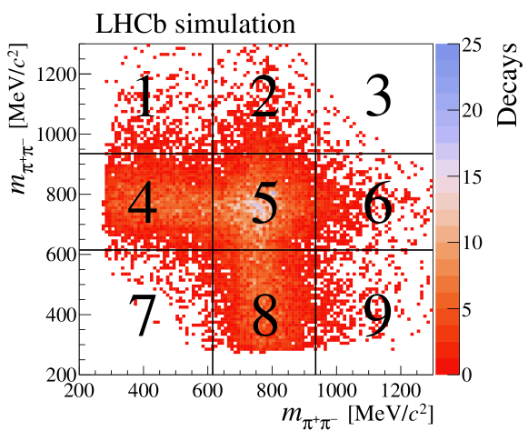
Figure 1: Two-dimensional distribution of the invariant masses $m_{{{\pi}^{+}}{{\pi}^{-}}}$ of the two oppositely charged two-pion combinations for simulated ${{B}^{0}_{s}}\rightarrow{\tau^{+}\tau^{-}}$ candidates. The distribution is symmetric by construction. The vertical and horizontal lines illustrate the sector boundaries.

For the ${B}\rightarrow{\tau^{+}\tau^{-}}$ modes, further requirements are imposed on two types of isolation variables that are able to discriminate signal from background from partially reconstructed decays with additional charged or neutral particles. The first class of isolation variables, based on the decision of a multivariate classifier trained on simulated signal and other $b$-hadron decays, discriminates against processes containing additional charged tracks that either make a good-quality vertex with any selected pion or $\tau$ candidate, or belong to the same $b$-hadron decay as the selected pion candidates. The second class of isolation variables is based on calorimeter activity due to neutral particles in a cone, defined in terms of the pseudorapidity and polar angle, centred on the $B$ candidate momentum.

In addition to the isolation variables, a method to perform an analytic reconstruction of the ${B}\rightarrow{\tau^{+}\tau^{-}}$ decay chain, described in detail in Refs. [37, 38], has been developed. It combines geometrical information about the decay and mass constraints on the particles (${B}$, $\tau$ and $\nu$) in the decay chain to calculate the $\tau$ momenta analytically. The possible solutions for the two $\tau$ momenta are found as solutions of a system of two coupled equations of second degree with two unknowns. The finite detector resolution and approximations made in the calculation prevent real solutions being found for a substantial fraction of the signal events. However, several intermediate quantities associated with the method are exploited to discriminate signal from background.

To make full use of the discrimination power present in the distributions of the selection variables, a requirement is added on the output of a neural network [39], built using seven variables: the $\tau^{\pm}$ candidate masses and decay times, a charged track isolation variable for the pions, a neutral isolation variable for the $B$ candidate, and one variable from the analytic reconstruction method, introduced in Ref. [38]. The classifier is trained on simulated ${B}\rightarrow{\tau^{+}\tau^{-}}$ decays, representing the signal, and data events from the signal-depleted region.

In order to determine the signal yield, a binned maximum likelihood fit is performed on the output of a second neural network (NN), built with 29 variables and using the same training samples. The NN inputs include the eight variables from the analytic reconstruction method listed in Ref. [38], further isolation variables, as well as kinematic and geometrical variables. The NN output is transformed to obtain a flat distribution for the signal over the range [0.0, 1.0], while the background peaks towards zero.

Varying the two-pion invariant mass sector boundaries, the signal region is optimised for the ${{B}^{0}_{s}}\rightarrow{\tau^{+}\tau^{-}}$ branching fraction limit using pseudoexperiments. The boundaries are set to 615 and 935 ${\mathrm{\,Me\kern-1.00006ptV\!/}c^{2}}$. The overall efficiency of the selection, determined using simulated ${B}_{(s)}^{0}\rightarrow{\tau^{+}\tau^{-}}$ decays, is approximately $2.2(2.4)\times 10^{-5}$, including the geometrical acceptance. Assuming the SM prediction, the number of ${{B}^{0}_{s}}\rightarrow{\tau^{+}\tau^{-}}$ decays expected in the signal region is 0.02.

After the selection, the signal, signal-depleted and control regions contain, respectively, 16%, 13% and 58% of the simulated signal decays. The corresponding fractions of selected candidates in data are 7%, 37% and 47%. Most signal decays fall into the control region, but the signal region, which contains about 14 700 candidates in data after the full selection, is more sensitive due to its lower background contamination. For the fit, ten equally sized bins of NN output in the range [0.0, 1.0] are considered, where the high NN region [0.7, 1.0] was not investigated until the fit strategy was fixed. The signal model is taken from the ${{B}^{0}_{s}}\rightarrow{\tau^{+}\tau^{-}}$ simulation, while the background model is taken from the data control region, correcting for the presence of expected signal events in this region. The fit model is given by

$$\mathcal{N}^{\text{SR}}_{\text{data}}=s\times\widehat{\mathcal{N}}^{\text{SR}}_{\text{sim}}+f_{b}\times\left(\mathcal{N}^{\text{CR}}_{\text{data}}-s\times\frac{{\varepsilon}^{\text{CR}}}{{\varepsilon}^{\text{SR}}}\times\widehat{\mathcal{N}}^{\text{CR}}_{\text{sim}}\right)\,,$$ (1)

where $\mathcal{N}^{\text{SR}}_{\text{sim/data}}$ ($\mathcal{N}^{\text{CR}}_{\text{sim/data}}$) is the NN output distribution in the signal (control) region from simulation/data, $s$ is the signal yield in the signal region, $f_{b}$ is a scaling factor for the background template, and ${\varepsilon}^{\text{SR}}$ (${\varepsilon}^{\text{CR}}$) is the signal efficiency in the signal (control) region. The quantities $s$ and $f_{b}$ are left free in the fit. The corresponding normalised distributions $\widehat{\mathcal{N}}^{\text{SR}}_{\text{sim}}$, $\widehat{\mathcal{N}}^{\text{CR}}_{\text{sim}}$ and $\widehat{\mathcal{N}}^{\text{CR}}_{\text{data}}$ are shown in Fig. 2.

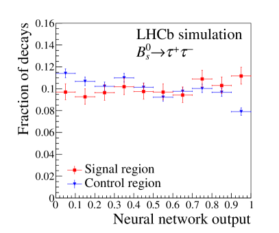
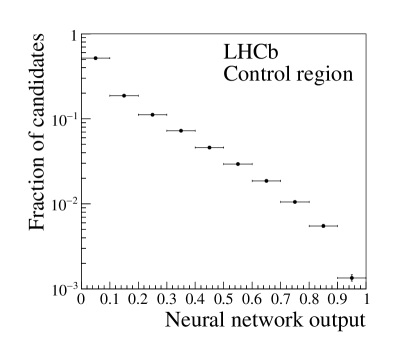
Figure 2: (left) Normalised NN output distribution in the signal ($\widehat{\mathcal{N}}^{\text{SR}}_{\text{sim}}$) and control ($\widehat{\mathcal{N}}^{\text{CR}}_{\text{sim}}$) region for ${{B}^{0}_{s}}\rightarrow{\tau^{+}\tau^{-}}$ simulated events. (right) Normalised NN output distribution in the data control region $\widehat{\mathcal{N}}^{\text{CR}}_{\text{data}}$. The uncertainties reflect the statistics of the (simulated) data.

The agreement between the background NN output distributions in the control and signal regions has been tested in different samples: in the data for the background-dominated NN output bins [0.0, 0.7], in a generic $b\overline{b}$ simulated sample and in several specific simulated background modes (such as ${{B}^{0}}\rightarrow{{D}^{-}}{{\pi}^{+}}{{\pi}^{-}}{{\pi}^{+}}$ with ${{D}^{-}}\rightarrow{{K}^{0}}{{\pi}^{-}}{{\pi}^{+}}{{\pi}^{-}}$, or ${{B}^{0}_{s}}\rightarrow{{D}^{-}_{s}}{{\pi}^{+}}{{\pi}^{-}}{{\pi}^{+}}$ with ${{D}^{-}_{s}}\rightarrow{\tau^{-}}\nu_{\tau}$). Within the statistical uncertainty, the distributions have been found to agree with each other in all cases. The background in the control region can therefore be used to characterise the background in the signal region.

Differences between the shapes of the background distribution in the signal and control regions of the data are the main sources of systematic uncertainties on the background model. These uncertainties are taken into account by allowing each bin in the $\mathcal{N}^{\text{CR}}_{\text{data}}$ distribution to vary according to a Gaussian constraint. The width of this Gaussian function is determined by splitting the control region into two approximately equally populated samples and taking, for each bin, the maximum difference between the NN outputs of the two subregions and the unsplit sample. The splitting is constructed to have one region more signal-like and one region more background-like.

The signal can be mismodelled in the simulation. The ${{B}^{0}}\rightarrow{{D}^{-}}{{D}^{+}_{s}}$ decay is used to compare data and simulation for the variables used in the NN. Ten variables are found to be slightly mismodelled and their distributions are corrected by weighting. The difference in the shape of the NN output distribution compared to the original unweighted sample is used to derive the associated systematic uncertainty. The fit procedure is validated with pseudoexperiments and is found to be unbiased. Assuming no signal contribution, the expected statistical (systematic) uncertainty on the signal yield is ${}^{+62}_{-40}\>(^{+40}_{-42})$. The fit result on data is shown in Fig. 3 and gives a signal yield $s=-23^{+63}_{-53}\mathrm{\,(stat)}^{+41}_{-40}\mathrm{\,(syst)}$, where the split between the statistical and systematic uncertainties is based on the ratio expected from pseudoexperiments.

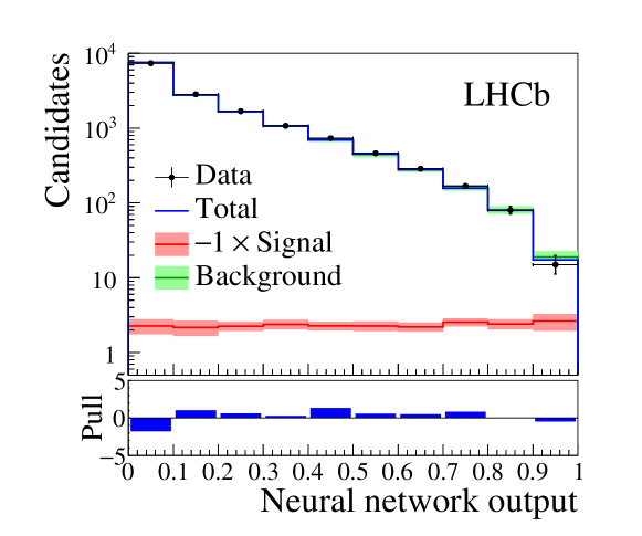
Figure 3: Distribution of the NN output in the signal region $\mathcal{N}^{\text{SR}}_{\text{data}}$ (black points), with the total fit result (blue line) and the background component (green line). The fitted ${{B}^{0}_{s}}\rightarrow{\tau^{+}\tau^{-}}$ signal component is negative and is therefore shown multiplied by $-1$ (red line). For each bin of the signal and background component the combined statistical and systematic uncertainty on the template is shown as a light-coloured band. The difference between data and fit divided by its uncertainty (pull) is shown underneath.

The ${{B}^{0}_{s}}\rightarrow{\tau^{+}\tau^{-}}$ signal yield is converted into a branching fraction using ${\mathcal{B}}({{B}^{0}_{s}}\rightarrow{\tau^{+}\tau^{-}})$ $=\alpha^{s}\times s$, with

$$\alpha^{s}\equiv\frac{\epsilon^{D^{-}D_{s}^{+}}\times{\mathcal{B}}({{B}^{0}}\rightarrow{{D}^{-}}{{D}^{+}_{s}})\times{\mathcal{B}}({{D}^{+}}\rightarrow{{K}^{-}}{{\pi}^{+}}{{\pi}^{+}})\times{\mathcal{B}}({{D}^{+}_{s}}\rightarrow{{K}^{+}}{{K}^{-}}{{\pi}^{+}})}{N_{{{D}^{-}}{{D}^{+}_{s}}}^{\text{obs}}\times\epsilon^{{\tau^{+}\tau^{-}}}\times\left[{\mathcal{B}}(\tau^{-}\rightarrow\pi^{-}\pi^{+}\pi^{-}\nu_{\tau})\right]^{2}}\times\frac{f_{d}}{f_{s}}\>,$$ (2)

where $\epsilon^{{\tau^{+}\tau^{-}}}$ and $\epsilon^{D^{-}D_{s}^{+}}$ are the combined efficiencies of trigger, reconstruction and selection of the signal and normalisation channels. The branching fractions used are ${\mathcal{B}}({{B}^{0}}\rightarrow{{D}^{-}}{{D}^{+}_{s}})=(7.5\pm 1.1)\times 10^{-3}$ [19], ${\mathcal{B}}({{D}^{-}}\rightarrow{{K}^{+}}{{\pi}^{-}}{{\pi}^{-}})=(9.46\pm 0.24)\%$ [18] and ${\mathcal{B}}({{D}^{+}_{s}}\rightarrow{{K}^{-}}{{K}^{+}}{{\pi}^{+}})=(5.45\pm 0.17)\%$ [18], and $f_{s}/f_{d}=0.259\pm 0.015$ [40, *LHCb-CONF-2013-011] is the ratio of ${B}^{0}_{s}$ to ${B}^{0}$ production fractions. The efficiencies are determined using simulation, applying correction factors derived from data. The ${B}^{0}$ $\rightarrow$ ${D}^{-}$ ${D}^{+}_{s}$ yield, $N_{D^{-}D_{s}^{+}}^{\text{obs}}$, is obtained from a fit to the mass distribution, which has four contributions: the ${B}^{0}$ $\rightarrow$ ${D}^{-}$ ${D}^{+}_{s}$ component, modelled by a Hypatia function [42], a combinatorial background component, described by an exponential function, and two partially reconstructed backgrounds, ${{B}^{0}}\rightarrow D^{*-}{{D}^{+}_{s}}$ and ${{B}^{0}}\rightarrow{{D}^{-}}D_{s}^{*+}$, modelled as in Ref. [43]. The resulting fit is shown in Fig. 4 and gives a yield of $N_{D^{-}D_{s}^{+}}^{\text{obs}}=10\,629\pm 114$, where the uncertainty is statistical.

Uncertainties on $\alpha^{s}$ arise from the ${{B}^{0}}\rightarrow D^{-}D_{s}^{+}$ fit model, the finite size of the simulated samples, the uncertainty from the corrections to the simulation and external inputs. The latter contribution, which includes the branching fractions and hadronisation fractions in Eq. (2), is dominant, giving a relative uncertainty of 17% on $\alpha^{s}$. The ${{B}^{0}}\rightarrow D^{-}D_{s}^{+}$ fit model is varied using the sum of two Gaussian functions with a common mean and power-law tails instead of the Hypatia function for the signal, a second-order Chebychev polynomial instead of an exponential function for the combinatorial background, and adding two other background components from ${{B}^{0}_{s}}\rightarrow D^{-}D_{s}^{*+}$ and ${{B}^{0}}\rightarrow a_{1}(1260)^{-}D_{s}^{*+}$ decays. The change in signal yield compared to the nominal fit is taken as a systematic uncertainty, adding the contributions from the four variations in quadrature. The overall relative uncertainty on $\alpha^{s}$ due to $N_{D^{-}D_{s}^{+}}^{\text{obs}}$ (including the fit uncertainty) is 1.7%. Corrections determined from $J/\psi\rightarrow\mu^{+}\mu^{-}$ and $D^{0}\rightarrow K^{-}\pi^{+}$ data control samples are applied for the tracking, PID and the hadronic hardware trigger efficiencies. The relative uncertainty on $\alpha^{s}$ due to selection efficiencies is 2.9%, taking into account both the limited size of the simulated samples and the systematic uncertainties. The normalisation factor is found to be $\alpha^{s}=(4.07\pm 0.70)\times 10^{-5}$.

The shapes of the NN output distributions and the selection efficiencies depend on the parametrisation used in the simulation to model the ${\tau^{-}}\rightarrow{{\pi}^{-}}{{\pi}^{+}}{{\pi}^{-}}\nu_{\tau}$ decay. The result obtained with the Tauola BaBar-tune model is therefore compared to available alternatives [44], which are based on CLEO data for the ${\tau^{-}}\rightarrow{{\pi}^{-}}\pi^{0}\pi^{0}\nu_{\tau}$ decay [45]. The selection efficiency for these alternative models can be up to 20% higher, due to different structures in the two-pion invariant mass, resulting in lower limits. Dependence of the NN signal output distribution on the $\tau$-decay model is found to be negligible. Since the alternative models are based on a different $\tau$ decay, the BaBar-tune model is chosen as default and no systematic uncertainty is assigned.

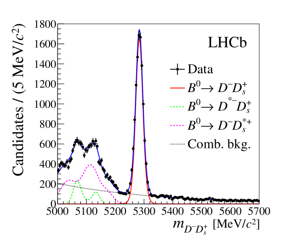
Figure 4: Invariant mass distribution of the reconstructed ${{B}^{0}}\rightarrow D^{-}D_{s}^{+}$ candidates in data (black points), together with the total fit result (blue line) used to determine the ${{B}^{0}}\rightarrow D^{-}D_{s}^{+}$ yield. The individual components are described in the text.

The signal yield obtained from the likelihood fit is translated into an upper limit on the ${{B}^{0}_{s}}\rightarrow{\tau^{+}\tau^{-}}$ branching fraction using the CL${}_{\text{s}}$ method [46, 47]. Assuming no contribution from ${{B}^{0}}\rightarrow{\tau^{+}\tau^{-}}$ decays, an upper limit is set on the ${{B}^{0}_{s}}\rightarrow{\tau^{+}\tau^{-}}$ branching fraction of $5.2\,(6.8)\times 10^{-3}$ at 90 (95)% CL. This is the first experimental limit on ${\mathcal{B}}({{B}^{0}_{s}}\rightarrow{\tau^{+}\tau^{-}})$. The analysis is repeated for the ${{B}^{0}}\rightarrow{\tau^{+}\tau^{-}}$ decay. The fit is performed by replacing the signal model with that derived from simulated ${{B}^{0}}\rightarrow{\tau^{+}\tau^{-}}$ decays, giving $s=-15^{+67}_{-56}\mathrm{\,(stat)}^{+44}_{-42}\mathrm{\,(syst)}$ [38]. The expected statistical (systematic) uncertainty on the signal yield is ${}^{+64}_{-58}\>(^{+41}_{-43})$. The corresponding normalisation factor is $\alpha^{d}=(1.16\pm 0.19)\times 10^{-5}$. The limit obtained is ${\mathcal{B}}({{B}^{0}}\rightarrow{\tau^{+}\tau^{-}})<1.6\,(2.1)\times 10^{-3}$ at 90 (95)% CL, which constitutes a factor 2.6 improvement with respect to the BaBar result [13] and is the current best limit on ${\mathcal{B}}({{B}^{0}}\rightarrow{\tau^{+}\tau^{-}})$.

Appendix A Supplemental material

In Section A.1, details about the analytic reconstruction method are given. Sections A.2 and A.3 contain additional results related to the ${{B}^{0}_{s}}\rightarrow{\tau^{+}\tau^{-}}$ and ${{B}^{0}}\rightarrow{\tau^{+}\tau^{-}}$ decay channels.

A.1 Reconstruction method

A method to perform an analytic reconstruction of the ${B}\rightarrow{\tau^{+}\tau^{-}}$ decay chain is described in the following and in detail in Ref. [37]. It combines geometrical information about the decay and sets mass constraints on the particles in the decay chain (${{B}^{0}_{s}}$, $\tau$ and $\nu$) to calculate the $\tau$ momenta analytically. In these calculations, Lorentz invariance is kept manifest and the possible values for the two $\tau$ momenta are found as analytic solutions of a system of two coupled equations of second degree in two unknowns. The only remaining degree of freedom is a single Lorentz scalar, introduced below as the angle $\theta$, measuring the asymmetry of the decay triangle in the decay-time space of the two $\tau$ leptons.

In the following, the unknown momenta of the $\tau^{\pm}$ leptons, the primary parameters of interest, are labelled by the four-vectors $p_{\pm}^{\mu}$; the ${{B}^{0}_{s}}\rightarrow{\tau^{+}\tau^{-}}$ decay plane is defined by the $B$ production vertex, i.e. the PV, and the two $\tau$ decay vertices; the three-vectors pointing from the PV to the $\tau^{\pm}$ decay vertices are labelled $\vec{w}_{\pm}$; the time intervals between the $B$ production and the $\tau^{\pm}$ decays, $w^{0}_{\pm}$, which cannot be measured, act as the temporal counterpart to $\vec{w}_{\pm}$. Together, they make the four-vectors $w_{\pm}^{\mu}=(w^{0}_{\pm},\vec{w}_{\pm})$. Introducing the notation

$$W\equiv(w_{+}^{\mu},w_{-}^{\mu})\>,\qquad P\equiv(p_{+}^{\mu},p_{-}^{\mu})\>,$$ (3)

the momenta $p_{\pm}^{\mu}$ can now be obtained from the coupled set of equations

$$W=H\cdot P$$ (4)

by imposing momentum conservation throughout the decay chain. Here

$$H\equiv\left(\begin{array}[]{cc}\frac{t_{B}}{m_{B}}+\frac{t_{\tau_{+}}}{m_{\tau}}&\frac{t_{B}}{m_{B}}\\ \frac{t_{B}}{m_{B}}&\frac{t_{B}}{m_{B}}+\frac{t_{\tau_{-}}}{m_{\tau}}\end{array}\right)$$ (5)

is given in terms of the $B$ and $\tau$ masses, $m_{i}$, and decay times, $t_{i}$. Using the on-shell and flight-direction constraints, it is possible to rewrite Eq. (4) in terms of a single unknown, chosen to be the rotation angle, $\theta$, that diagonalises the matrix $H$. Thanks to this transformation, solving Eq. (4) becomes equivalent to finding the roots of a fourth-order polynomial

$$\mathcal{P}^{(4)}(\xi)=\sum_{i=0}^{4}a_{i}(\theta)\xi^{i}=0\>,$$ (6)

where explicit expressions for the coefficients $a_{i}(\theta)$ in terms of $\theta$ and measurable quantities are given in Appendix D of Ref. [37].

Even though it is possible, in principle, to exactly determine the angle $\theta$, a different approach has been used, because of the high complexity of the trigonometric equations involved. The value of the angle $\theta$ is in fact approximated in the calculation of the complex solutions $\xi_{1}$, …, $\xi_{4}$. Three approximations have been considered in Ref. [37]. They are

1. $\theta=\langle\theta\rangle=\pi/4$, representing the case where both $\tau$ leptons have the same decay time.

2. $\theta=\bar{\theta}$, where $\bar{\theta}$ is the angle diagonalising the matrix

   $$\overline{H}\equiv\left(\begin{array}[]{cc}1+\frac{|\vec{w}_{+}|}{|\vec{w}_{+}+\vec{w}_{-}|}&1\\ 1&1+\frac{|\vec{w}_{-}|}{|\vec{w}_{+}+\vec{w}_{-}|}\end{array}\right)$$ (7)

3. $\theta=\theta^{*}$, where $\theta^{*}$ is the result of applying iterative corrections to $\theta=\bar{\theta}$.

These approximations, together with the finite detector resolution, prevent having real solutions for a substantial fraction of the signal events. Nonetheless, quantities appearing in intermediate calculations, though not having immediate physical meaning, have been found useful to discriminate between signal and background. The most powerful of these variables are exploited in the two neural networks that are used in the candidate selection. The variable

• $\mathcal{R}e[|\vec{\tilde{p}}_{+}(\theta=\bar{\theta},\xi_{3})|]$

is used by both the first and second NN, while the seven variables

• $\mathcal{I}m[|\vec{\tilde{p}}_{+}(\theta=\theta^{\star},\xi_{1})|]$,

• $\mathcal{I}m[\tilde{p}_{+}(\theta=\theta^{\star},\xi_{1})\tilde{p}_{-}(\theta=\theta^{\star},\xi_{1})]$,

• $\mathcal{I}m[\tilde{p}_{+}(\theta=\theta^{\star},\xi_{3})\tilde{p}_{-}(\theta=\theta^{\star},\xi_{3})]$,

• $\mathcal{R}e[\tilde{p}_{+}(\theta=\pi/4,\xi_{1})\tilde{p}_{-}(\theta=\pi/4,\xi_{1})]$,

• $\mathcal{R}e[\xi_{1}(\theta=\theta^{*})]$,

• $\bar{\theta}$,

• $p_{+}\cdot p_{-}$,

are used by the second NN. Here $\tilde{p}^{2}_{\pm}\equiv M^{2}_{\pm}=m^{2}_{\tau}\pm\sin(2\theta)\hat{s}$, and $\hat{s}\equiv p_{+}\cdot p_{-}$ (for signal events $\hat{s}=\frac{M^{2}_{B}-2m^{2}_{\tau}}{2}$).

A.2 Additional ${{B}^{0}_{s}}$ fit result

Figure 5 shows the fit result using only the background model. A likelihood-ratio test is performed comparing the nominal fit with the background-only alternative. The $p$-value of the likelihood-ratio test is 0.06, and the associated $z$-score is 1.60, showing that the data are consistent with the background-only hypothesis. Figure 6 shows the profile likelihood of the nominal fit. Figure 7 shows the expected and observed CL${}_{\text{s}}$ values as a function of the branching fraction. The expected limit for the ${{B}^{0}_{s}}$ mode is ${\mathcal{B}}({{B}^{0}_{s}}\rightarrow{\tau^{+}\tau^{-}})<5.7\,(7.4)\times 10^{-3}$ at 90 (95)% CL.

A.3 Additional ${{B}^{0}}$ fit result

The NN output distributions for simulated ${{B}^{0}}\rightarrow{\tau^{+}\tau^{-}}$ decays in the signal and control regions are shown in Fig. 8. The fit result, assuming no contribution from ${{B}^{0}_{s}}\rightarrow{\tau^{+}\tau^{-}}$ decays, is shown in Fig. 9, and Fig. 10 shows the expected and observed CL${}_{\text{s}}$ values as a function of the branching fraction. The expected limit for the ${{B}^{0}}$ mode is ${\mathcal{B}}({{B}^{0}}\rightarrow{\tau^{+}\tau^{-}})<1.7\,(2.1)\times 10^{-3}$ at 90 (95)% CL.

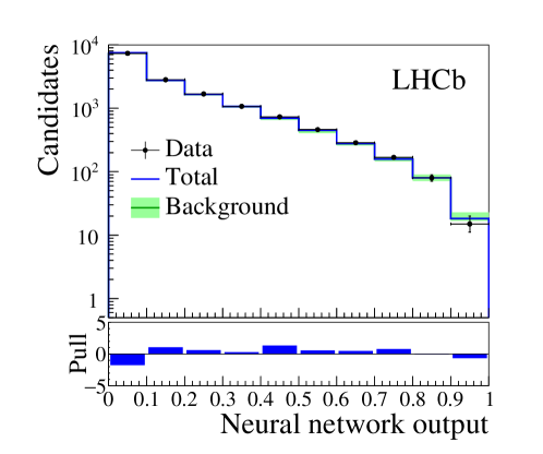
Figure 5: Distribution of the NN output in the signal region $\mathcal{N}^{\text{SR}}_{\text{data}}$ (black points), with the total fit result (blue line), and the background component (green line). Shown is the fit using the “background only” model. For each bin of the background component the combined statistical and systematic uncertainty is shown as a light-coloured band. The difference between data and fit divided by its uncertainty (pull) is shown underneath.

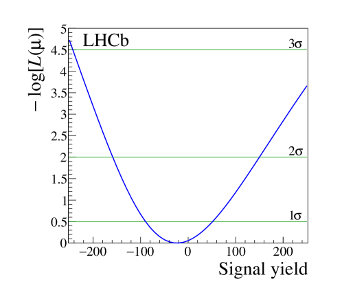
Figure 6: Profile likelihood scan of the ${{B}^{0}_{s}}\rightarrow{\tau^{+}\tau^{-}}$ signal yield. The intersections of the likelihood curve with the horizontal lines define the 68.3%, 95.4% and 99.7% likelihood intervals.

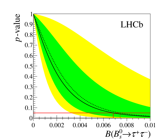
Figure 7: The $p$-value derived with the CL${}_{\text{s}}$ method as a function of ${\mathcal{B}}({{B}^{0}_{s}}\rightarrow{\tau^{+}\tau^{-}})$. Expected (observed) values are shown by a dashed (full) black line. The green (yellow) band covers the regions of 68% and 95% confidence for the expected limit. The red horizontal line corresponds to the limit at 95% CL.

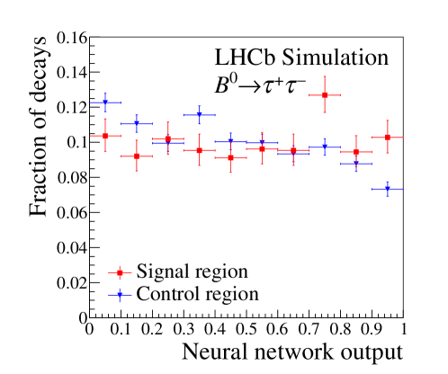
Figure 8: Normalised NN output distribution in the signal ($\widehat{\mathcal{N}}^{\text{SR}}_{\text{sim}}$) and control ($\widehat{\mathcal{N}}^{\text{CR}}_{\text{sim}}$) region for ${{B}^{0}}\rightarrow{\tau^{+}\tau^{-}}$ simulated events.

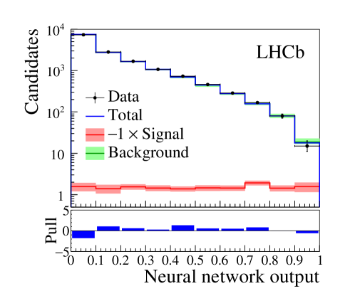
Figure 9: Fit results for ${{B}^{0}}\rightarrow{\tau^{+}\tau^{-}}$. Distribution $\mathcal{N}^{\text{SR}}_{\text{data}}$ (black points), overlaid with the total fit result (blue line), and background component (green line), assuming all signal events originate from ${{B}^{0}}\rightarrow{\tau^{+}\tau^{-}}$ decays. The ${{B}^{0}}\rightarrow{\tau^{+}\tau^{-}}$ signal component is also shown (red line), multiplied by $-1$. For each bin of the signal and background component the combined statistical and systematic uncertainty is shown as a light-coloured band. The difference between data and fit divided by its uncertainty (pull) is shown underneath.

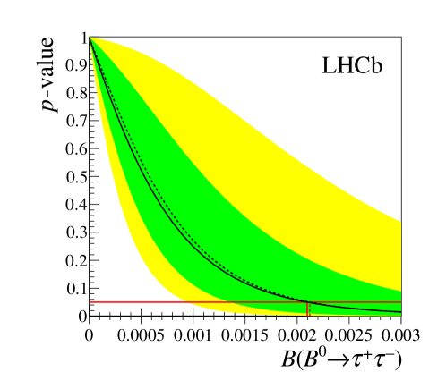
Figure 10: The $p$-value derived with the CL${}_{\text{s}}$ method as a function of ${\mathcal{B}}({{B}^{0}}\rightarrow{\tau^{+}\tau^{-}}$). Expected (observed) values are shown by a dashed (full) black line. The green (yellow) band covers the regions of 68% and 95% confidence for the expected limit. The red horizontal line corresponds to the limit at 95% CL.

LHCb collaboration

R. Aaij⁴⁰, B. Adeva³⁹, M. Adinolfi⁴⁸, Z. Ajaltouni⁵, S. Akar⁵⁹, J. Albrecht¹⁰, F. Alessio⁴⁰, M. Alexander⁵³, S. Ali⁴³, G. Alkhazov³¹, P. Alvarez Cartelle⁵⁵, A.A. Alves Jr⁵⁹, S. Amato², S. Amerio²³, Y. Amhis⁷, L. An³, L. Anderlini¹⁸, G. Andreassi⁴¹, M. Andreotti^17,g, J.E. Andrews⁶⁰, R.B. Appleby⁵⁶, F. Archilli⁴³, P. d’Argent¹², J. Arnau Romeu⁶, A. Artamonov³⁷, M. Artuso⁶¹, E. Aslanides⁶, G. Auriemma²⁶, M. Baalouch⁵, I. Babuschkin⁵⁶, S. Bachmann¹², J.J. Back⁵⁰, A. Badalov³⁸, C. Baesso⁶², S. Baker⁵⁵, V. Balagura^7,c, W. Baldini¹⁷, A. Baranov³⁵, R.J. Barlow⁵⁶, C. Barschel⁴⁰, S. Barsuk⁷, W. Barter⁵⁶, F. Baryshnikov³², M. Baszczyk²⁷, V. Batozskaya²⁹, B. Batsukh⁶¹, V. Battista⁴¹, A. Bay⁴¹, L. Beaucourt⁴, J. Beddow⁵³, F. Bedeschi²⁴, I. Bediaga¹, A. Beiter⁶¹, L.J. Bel⁴³, V. Bellee⁴¹, N. Belloli^21,i, K. Belous³⁷, I. Belyaev³², E. Ben-Haim⁸, G. Bencivenni¹⁹, S. Benson⁴³, S. Beranek⁹, A. Berezhnoy³³, R. Bernet⁴², A. Bertolin²³, C. Betancourt⁴², F. Betti¹⁵, M.-O. Bettler⁴⁰, M. van Beuzekom⁴³, Ia. Bezshyiko⁴², S. Bifani⁴⁷, P. Billoir⁸, A. Birnkraut¹⁰, A. Bitadze⁵⁶, A. Bizzeti^18,u, T. Blake⁵⁰, F. Blanc⁴¹, J. Blouw^11,†, S. Blusk⁶¹, V. Bocci²⁶, T. Boettcher⁵⁸, A. Bondar^36,w, N. Bondar³¹, W. Bonivento¹⁶, I. Bordyuzhin³², A. Borgheresi^21,i, S. Borghi⁵⁶, M. Borisyak³⁵, M. Borsato³⁹, F. Bossu⁷, M. Boubdir⁹, T.J.V. Bowcock⁵⁴, E. Bowen⁴², C. Bozzi^17,40, S. Braun¹², T. Britton⁶¹, J. Brodzicka⁵⁶, E. Buchanan⁴⁸, C. Burr⁵⁶, A. Bursche², J. Buytaert⁴⁰, S. Cadeddu¹⁶, R. Calabrese^17,g, M. Calvi^21,i, M. Calvo Gomez^38,m, A. Camboni³⁸, P. Campana¹⁹, D.H. Campora Perez⁴⁰, L. Capriotti⁵⁶, A. Carbone^15,e, G. Carboni^25,j, R. Cardinale^20,h, A. Cardini¹⁶, P. Carniti^21,i, L. Carson⁵², K. Carvalho Akiba², G. Casse⁵⁴, L. Cassina^21,i, L. Castillo Garcia⁴¹, M. Cattaneo⁴⁰, G. Cavallero²⁰, R. Cenci^24,t, D. Chamont⁷, M. Charles⁸, Ph. Charpentier⁴⁰, G. Chatzikonstantinidis⁴⁷, M. Chefdeville⁴, S. Chen⁵⁶, S.-F. Cheung⁵⁷, V. Chobanova³⁹, M. Chrzaszcz^42,27, A. Chubykin³¹, X. Cid Vidal³⁹, G. Ciezarek⁴³, P.E.L. Clarke⁵², M. Clemencic⁴⁰, H.V. Cliff⁴⁹, J. Closier⁴⁰, V. Coco⁵⁹, J. Cogan⁶, E. Cogneras⁵, V. Cogoni^16,f, L. Cojocariu³⁰, P. Collins⁴⁰, A. Comerma-Montells¹², A. Contu⁴⁰, A. Cook⁴⁸, G. Coombs⁴⁰, S. Coquereau³⁸, G. Corti⁴⁰, M. Corvo^17,g, C.M. Costa Sobral⁵⁰, B. Couturier⁴⁰, G.A. Cowan⁵², D.C. Craik⁵², A. Crocombe⁵⁰, M. Cruz Torres⁶², S. Cunliffe⁵⁵, R. Currie⁵², C. D’Ambrosio⁴⁰, F. Da Cunha Marinho², E. Dall’Occo⁴³, J. Dalseno⁴⁸, P.N.Y. David⁴³, A. Davis³, K. De Bruyn⁶, S. De Capua⁵⁶, M. De Cian¹², J.M. De Miranda¹, L. De Paula², M. De Serio^14,d, P. De Simone¹⁹, C.T. Dean⁵³, D. Decamp⁴, M. Deckenhoff¹⁰, L. Del Buono⁸, H.-P. Dembinski¹¹, M. Demmer¹⁰, A. Dendek²⁸, D. Derkach³⁵, O. Deschamps⁵, F. Dettori⁵⁴, B. Dey²², A. Di Canto⁴⁰, P. Di Nezza¹⁹, H. Dijkstra⁴⁰, F. Dordei⁴⁰, M. Dorigo⁴¹, A. Dosil Suárez³⁹, A. Dovbnya⁴⁵, K. Dreimanis⁵⁴, L. Dufour⁴³, G. Dujany⁵⁶, K. Dungs⁴⁰, P. Durante⁴⁰, R. Dzhelyadin³⁷, M. Dziewiecki¹², A. Dziurda⁴⁰, A. Dzyuba³¹, N. Déléage⁴, S. Easo⁵¹, M. Ebert⁵², U. Egede⁵⁵, V. Egorychev³², S. Eidelman^36,w, S. Eisenhardt⁵², U. Eitschberger¹⁰, R. Ekelhof¹⁰, L. Eklund⁵³, S. Ely⁶¹, S. Esen¹², H.M. Evans⁴⁹, T. Evans⁵⁷, A. Falabella¹⁵, N. Farley⁴⁷, S. Farry⁵⁴, R. Fay⁵⁴, D. Fazzini^21,i, D. Ferguson⁵², G. Fernandez³⁸, A. Fernandez Prieto³⁹, F. Ferrari¹⁵, F. Ferreira Rodrigues², M. Ferro-Luzzi⁴⁰, S. Filippov³⁴, R.A. Fini¹⁴, M. Fiore^17,g, M. Fiorini^17,g, M. Firlej²⁸, C. Fitzpatrick⁴¹, T. Fiutowski²⁸, F. Fleuret^7,b, K. Fohl⁴⁰, M. Fontana^16,40, F. Fontanelli^20,h, D.C. Forshaw⁶¹, R. Forty⁴⁰, V. Franco Lima⁵⁴, M. Frank⁴⁰, C. Frei⁴⁰, J. Fu^22,q, W. Funk⁴⁰, E. Furfaro^25,j, C. Färber⁴⁰, A. Gallas Torreira³⁹, D. Galli^15,e, S. Gallorini²³, S. Gambetta⁵², M. Gandelman², P. Gandini⁵⁷, Y. Gao³, L.M. Garcia Martin⁶⁹, J. García Pardiñas³⁹, J. Garra Tico⁴⁹, L. Garrido³⁸, P.J. Garsed⁴⁹, D. Gascon³⁸, C. Gaspar⁴⁰, L. Gavardi¹⁰, G. Gazzoni⁵, D. Gerick¹², E. Gersabeck¹², M. Gersabeck⁵⁶, T. Gershon⁵⁰, Ph. Ghez⁴, S. Gianì⁴¹, V. Gibson⁴⁹, O.G. Girard⁴¹, L. Giubega³⁰, K. Gizdov⁵², V.V. Gligorov⁸, D. Golubkov³², A. Golutvin^55,40, A. Gomes^1,a, I.V. Gorelov³³, C. Gotti^21,i, E. Govorkova⁴³, R. Graciani Diaz³⁸, L.A. Granado Cardoso⁴⁰, E. Graugés³⁸, E. Graverini⁴², G. Graziani¹⁸, A. Grecu³⁰, R. Greim⁹, P. Griffith¹⁶, L. Grillo^21,40,i, B.R. Gruberg Cazon⁵⁷, O. Grünberg⁶⁷, E. Gushchin³⁴, Yu. Guz³⁷, T. Gys⁴⁰, C. Göbel⁶², T. Hadavizadeh⁵⁷, C. Hadjivasiliou⁵, G. Haefeli⁴¹, C. Haen⁴⁰, S.C. Haines⁴⁹, B. Hamilton⁶⁰, X. Han¹², S. Hansmann-Menzemer¹², N. Harnew⁵⁷, S.T. Harnew⁴⁸, J. Harrison⁵⁶, M. Hatch⁴⁰, J. He⁶³, T. Head⁴¹, A. Heister⁹, K. Hennessy⁵⁴, P. Henrard⁵, L. Henry⁶⁹, E. van Herwijnen⁴⁰, M. Heß⁶⁷, A. Hicheur², D. Hill⁵⁷, C. Hombach⁵⁶, H. Hopchev⁴¹, Z.-C. Huard⁵⁹, W. Hulsbergen⁴³, T. Humair⁵⁵, M. Hushchyn³⁵, D. Hutchcroft⁵⁴, M. Idzik²⁸, P. Ilten⁵⁸, R. Jacobsson⁴⁰, J. Jalocha⁵⁷, E. Jans⁴³, A. Jawahery⁶⁰, F. Jiang³, M. John⁵⁷, D. Johnson⁴⁰, C.R. Jones⁴⁹, C. Joram⁴⁰, B. Jost⁴⁰, N. Jurik⁵⁷, S. Kandybei⁴⁵, M. Karacson⁴⁰, J.M. Kariuki⁴⁸, S. Karodia⁵³, M. Kecke¹², M. Kelsey⁶¹, M. Kenzie⁴⁹, T. Ketel⁴⁴, E. Khairullin³⁵, B. Khanji¹², C. Khurewathanakul⁴¹, T. Kirn⁹, S. Klaver⁵⁶, K. Klimaszewski²⁹, T. Klimkovich¹¹, S. Koliiev⁴⁶, M. Kolpin¹², I. Komarov⁴¹, R. Kopecna¹², P. Koppenburg⁴³, A. Kosmyntseva³², S. Kotriakhova³¹, A. Kozachuk³³, M. Kozeiha⁵, L. Kravchuk³⁴, M. Kreps⁵⁰, P. Krokovny^36,w, F. Kruse¹⁰, W. Krzemien²⁹, W. Kucewicz^27,l, M. Kucharczyk²⁷, V. Kudryavtsev^36,w, A.K. Kuonen⁴¹, K. Kurek²⁹, T. Kvaratskheliya^32,40, D. Lacarrere⁴⁰, G. Lafferty⁵⁶, A. Lai¹⁶, G. Lanfranchi¹⁹, C. Langenbruch⁹, T. Latham⁵⁰, C. Lazzeroni⁴⁷, R. Le Gac⁶, J. van Leerdam⁴³, A. Leflat^33,40, J. Lefrançois⁷, R. Lefèvre⁵, F. Lemaitre⁴⁰, E. Lemos Cid³⁹, O. Leroy⁶, T. Lesiak²⁷, B. Leverington¹², T. Li³, Y. Li⁷, Z. Li⁶¹, T. Likhomanenko^35,68, R. Lindner⁴⁰, F. Lionetto⁴², X. Liu³, D. Loh⁵⁰, I. Longstaff⁵³, J.H. Lopes², D. Lucchesi^23,o, M. Lucio Martinez³⁹, H. Luo⁵², A. Lupato²³, E. Luppi^17,g, O. Lupton⁴⁰, A. Lusiani²⁴, X. Lyu⁶³, F. Machefert⁷, F. Maciuc³⁰, O. Maev³¹, K. Maguire⁵⁶, S. Malde⁵⁷, A. Malinin⁶⁸, T. Maltsev³⁶, G. Manca^16,f, G. Mancinelli⁶, P. Manning⁶¹, J. Maratas^5,v, J.F. Marchand⁴, U. Marconi¹⁵, C. Marin Benito³⁸, M. Marinangeli⁴¹, P. Marino^24,t, J. Marks¹², G. Martellotti²⁶, M. Martin⁶, M. Martinelli⁴¹, D. Martinez Santos³⁹, F. Martinez Vidal⁶⁹, D. Martins Tostes², L.M. Massacrier⁷, A. Massafferri¹, R. Matev⁴⁰, A. Mathad⁵⁰, Z. Mathe⁴⁰, C. Matteuzzi²¹, A. Mauri⁴², E. Maurice^7,b, B. Maurin⁴¹, A. Mazurov⁴⁷, M. McCann^55,40, A. McNab⁵⁶, R. McNulty¹³, B. Meadows⁵⁹, F. Meier¹⁰, D. Melnychuk²⁹, M. Merk⁴³, A. Merli^22,q, E. Michielin²³, D.A. Milanes⁶⁶, M.-N. Minard⁴, D.S. Mitzel¹², A. Mogini⁸, J. Molina Rodriguez¹, I.A. Monroy⁶⁶, S. Monteil⁵, M. Morandin²³, A. Mordà⁶, M.J. Morello^24,t, O. Morgunova⁶⁸, J. Moron²⁸, A.B. Morris⁵², R. Mountain⁶¹, F. Muheim⁵², M. Mulder⁴³, M. Mussini¹⁵, D. Müller⁵⁶, J. Müller¹⁰, K. Müller⁴², V. Müller¹⁰, P. Naik⁴⁸, T. Nakada⁴¹, R. Nandakumar⁵¹, A. Nandi⁵⁷, I. Nasteva², M. Needham⁵², N. Neri^22,40, S. Neubert¹², N. Neufeld⁴⁰, M. Neuner¹², T.D. Nguyen⁴¹, C. Nguyen-Mau^41,n, S. Nieswand⁹, R. Niet¹⁰, N. Nikitin³³, T. Nikodem¹², A. Nogay⁶⁸, A. Novoselov³⁷, D.P. O’Hanlon⁵⁰, A. Oblakowska-Mucha²⁸, V. Obraztsov³⁷, S. Ogilvy¹⁹, R. Oldeman^16,f, C.J.G. Onderwater⁷⁰, A. Ossowska²⁷, J.M. Otalora Goicochea², P. Owen⁴², A. Oyanguren⁶⁹, P.R. Pais⁴¹, A. Palano^14,d, M. Palutan^19,40, A. Papanestis⁵¹, M. Pappagallo^14,d, L.L. Pappalardo^17,g, C. Pappenheimer⁵⁹, W. Parker⁶⁰, C. Parkes⁵⁶, G. Passaleva¹⁸, A. Pastore^14,d, M. Patel⁵⁵, C. Patrignani^15,e, A. Pearce⁴⁰, A. Pellegrino⁴³, G. Penso²⁶, M. Pepe Altarelli⁴⁰, S. Perazzini⁴⁰, P. Perret⁵, L. Pescatore⁴¹, K. Petridis⁴⁸, A. Petrolini^20,h, A. Petrov⁶⁸, M. Petruzzo^22,q, E. Picatoste Olloqui³⁸, B. Pietrzyk⁴, M. Pikies²⁷, D. Pinci²⁶, A. Pistone²⁰, A. Piucci¹², V. Placinta³⁰, S. Playfer⁵², M. Plo Casasus³⁹, T. Poikela⁴⁰, F. Polci⁸, M Poli Lener¹⁹, A. Poluektov^50,36, I. Polyakov⁶¹, E. Polycarpo², G.J. Pomery⁴⁸, S. Ponce⁴⁰, A. Popov³⁷, D. Popov^11,40, B. Popovici³⁰, S. Poslavskii³⁷, C. Potterat², E. Price⁴⁸, J. Prisciandaro³⁹, C. Prouve⁴⁸, V. Pugatch⁴⁶, A. Puig Navarro⁴², G. Punzi^24,p, C. Qian⁶³, W. Qian⁵⁰, R. Quagliani^7,48, B. Rachwal²⁸, J.H. Rademacker⁴⁸, M. Rama²⁴, M. Ramos Pernas³⁹, M.S. Rangel², I. Raniuk⁴⁵, F. Ratnikov³⁵, G. Raven⁴⁴, F. Redi⁵⁵, S. Reichert¹⁰, A.C. dos Reis¹, C. Remon Alepuz⁶⁹, V. Renaudin⁷, S. Ricciardi⁵¹, S. Richards⁴⁸, M. Rihl⁴⁰, K. Rinnert⁵⁴, V. Rives Molina³⁸, P. Robbe⁷, A.B. Rodrigues¹, E. Rodrigues⁵⁹, J.A. Rodriguez Lopez⁶⁶, P. Rodriguez Perez^56,†, A. Rogozhnikov³⁵, S. Roiser⁴⁰, A. Rollings⁵⁷, V. Romanovskiy³⁷, A. Romero Vidal³⁹, J.W. Ronayne¹³, M. Rotondo¹⁹, M.S. Rudolph⁶¹, T. Ruf⁴⁰, P. Ruiz Valls⁶⁹, J.J. Saborido Silva³⁹, E. Sadykhov³², N. Sagidova³¹, B. Saitta^16,f, V. Salustino Guimaraes¹, D. Sanchez Gonzalo³⁸, C. Sanchez Mayordomo⁶⁹, B. Sanmartin Sedes³⁹, R. Santacesaria²⁶, C. Santamarina Rios³⁹, M. Santimaria¹⁹, E. Santovetti^25,j, A. Sarti^19,k, C. Satriano^26,s, A. Satta²⁵, D.M. Saunders⁴⁸, D. Savrina^32,33, S. Schael⁹, M. Schellenberg¹⁰, M. Schiller⁵³, H. Schindler⁴⁰, M. Schlupp¹⁰, M. Schmelling¹¹, T. Schmelzer¹⁰, B. Schmidt⁴⁰, O. Schneider⁴¹, A. Schopper⁴⁰, H.F. Schreiner⁵⁹, K. Schubert¹⁰, M. Schubiger⁴¹, M.-H. Schune⁷, R. Schwemmer⁴⁰, B. Sciascia¹⁹, A. Sciubba^26,k, A. Semennikov³², A. Sergi⁴⁷, N. Serra⁴², J. Serrano⁶, L. Sestini²³, P. Seyfert²¹, M. Shapkin³⁷, I. Shapoval⁴⁵, Y. Shcheglov³¹, T. Shears⁵⁴, L. Shekhtman^36,w, V. Shevchenko⁶⁸, B.G. Siddi^17,40, R. Silva Coutinho⁴², L. Silva de Oliveira², G. Simi^23,o, S. Simone^14,d, M. Sirendi⁴⁹, N. Skidmore⁴⁸, T. Skwarnicki⁶¹, E. Smith⁵⁵, I.T. Smith⁵², J. Smith⁴⁹, M. Smith⁵⁵, l. Soares Lavra¹, M.D. Sokoloff⁵⁹, F.J.P. Soler⁵³, B. Souza De Paula², B. Spaan¹⁰, P. Spradlin⁵³, S. Sridharan⁴⁰, F. Stagni⁴⁰, M. Stahl¹², S. Stahl⁴⁰, P. Stefko⁴¹, S. Stefkova⁵⁵, O. Steinkamp⁴², S. Stemmle¹², O. Stenyakin³⁷, H. Stevens¹⁰, S. Stoica³⁰, S. Stone⁶¹, B. Storaci⁴², S. Stracka^24,p, M.E. Stramaglia⁴¹, M. Straticiuc³⁰, U. Straumann⁴², L. Sun⁶⁴, W. Sutcliffe⁵⁵, K. Swientek²⁸, V. Syropoulos⁴⁴, M. Szczekowski²⁹, T. Szumlak²⁸, S. T’Jampens⁴, A. Tayduganov⁶, T. Tekampe¹⁰, G. Tellarini^17,g, F. Teubert⁴⁰, E. Thomas⁴⁰, J. van Tilburg⁴³, M.J. Tilley⁵⁵, V. Tisserand⁴, M. Tobin⁴¹, S. Tolk⁴⁹, L. Tomassetti^17,g, D. Tonelli²⁴, S. Topp-Joergensen⁵⁷, F. Toriello⁶¹, R. Tourinho Jadallah Aoude¹, E. Tournefier⁴, S. Tourneur⁴¹, K. Trabelsi⁴¹, M. Traill⁵³, M.T. Tran⁴¹, M. Tresch⁴², A. Trisovic⁴⁰, A. Tsaregorodtsev⁶, P. Tsopelas⁴³, A. Tully⁴⁹, N. Tuning⁴³, A. Ukleja²⁹, A. Ustyuzhanin³⁵, U. Uwer¹², C. Vacca^16,f, V. Vagnoni^15,40, A. Valassi⁴⁰, S. Valat⁴⁰, G. Valenti¹⁵, R. Vazquez Gomez¹⁹, P. Vazquez Regueiro³⁹, S. Vecchi¹⁷, M. van Veghel⁴³, J.J. Velthuis⁴⁸, M. Veltri^18,r, G. Veneziano⁵⁷, A. Venkateswaran⁶¹, T.A. Verlage⁹, M. Vernet⁵, M. Vesterinen¹², J.V. Viana Barbosa⁴⁰, B. Viaud⁷, D.  Vieira⁶³, M. Vieites Diaz³⁹, H. Viemann⁶⁷, X. Vilasis-Cardona^38,m, M. Vitti⁴⁹, V. Volkov³³, A. Vollhardt⁴², B. Voneki⁴⁰, A. Vorobyev³¹, V. Vorobyev^36,w, C. Voß⁹, J.A. de Vries⁴³, C. Vázquez Sierra³⁹, R. Waldi⁶⁷, C. Wallace⁵⁰, R. Wallace¹³, J. Walsh²⁴, J. Wang⁶¹, D.R. Ward⁴⁹, H.M. Wark⁵⁴, N.K. Watson⁴⁷, D. Websdale⁵⁵, A. Weiden⁴², M. Whitehead⁴⁰, J. Wicht⁵⁰, G. Wilkinson^57,40, M. Wilkinson⁶¹, M. Williams⁴⁰, M.P. Williams⁴⁷, M. Williams⁵⁸, T. Williams⁴⁷, F.F. Wilson⁵¹, J. Wimberley⁶⁰, M.A. Winn⁷, J. Wishahi¹⁰, W. Wislicki²⁹, M. Witek²⁷, G. Wormser⁷, S.A. Wotton⁴⁹, K. Wraight⁵³, K. Wyllie⁴⁰, Y. Xie⁶⁵, Z. Xing⁶¹, Z. Xu⁴, Z. Yang³, Z Yang⁶⁰, Y. Yao⁶¹, H. Yin⁶⁵, J. Yu⁶⁵, X. Yuan^36,w, O. Yushchenko³⁷, K.A. Zarebski⁴⁷, M. Zavertyaev^11,c, L. Zhang³, Y. Zhang⁷, A. Zhelezov¹², Y. Zheng⁶³, X. Zhu³, V. Zhukov³³, S. Zucchelli¹⁵.

¹Centro Brasileiro de Pesquisas Físicas (CBPF), Rio de Janeiro, Brazil
²Universidade Federal do Rio de Janeiro (UFRJ), Rio de Janeiro, Brazil
³Center for High Energy Physics, Tsinghua University, Beijing, China
⁴LAPP, Université Savoie Mont-Blanc, CNRS/IN2P3, Annecy-Le-Vieux, France
⁵Clermont Université, Université Blaise Pascal, CNRS/IN2P3, LPC, Clermont-Ferrand, France
⁶CPPM, Aix-Marseille Université, CNRS/IN2P3, Marseille, France
⁷LAL, Université Paris-Sud, CNRS/IN2P3, Orsay, France
⁸LPNHE, Université Pierre et Marie Curie, Université Paris Diderot, CNRS/IN2P3, Paris, France
⁹I. Physikalisches Institut, RWTH Aachen University, Aachen, Germany
¹⁰Fakultät Physik, Technische Universität Dortmund, Dortmund, Germany
¹¹Max-Planck-Institut für Kernphysik (MPIK), Heidelberg, Germany
¹²Physikalisches Institut, Ruprecht-Karls-Universität Heidelberg, Heidelberg, Germany
¹³School of Physics, University College Dublin, Dublin, Ireland
¹⁴Sezione INFN di Bari, Bari, Italy
¹⁵Sezione INFN di Bologna, Bologna, Italy
¹⁶Sezione INFN di Cagliari, Cagliari, Italy
¹⁷Sezione INFN di Ferrara, Ferrara, Italy
¹⁸Sezione INFN di Firenze, Firenze, Italy
¹⁹Laboratori Nazionali dell’INFN di Frascati, Frascati, Italy
²⁰Sezione INFN di Genova, Genova, Italy
²¹Sezione INFN di Milano Bicocca, Milano, Italy
²²Sezione INFN di Milano, Milano, Italy
²³Sezione INFN di Padova, Padova, Italy
²⁴Sezione INFN di Pisa, Pisa, Italy
²⁵Sezione INFN di Roma Tor Vergata, Roma, Italy
²⁶Sezione INFN di Roma La Sapienza, Roma, Italy
²⁷Henryk Niewodniczanski Institute of Nuclear Physics Polish Academy of Sciences, Kraków, Poland
²⁸AGH - University of Science and Technology, Faculty of Physics and Applied Computer Science, Kraków, Poland
²⁹National Center for Nuclear Research (NCBJ), Warsaw, Poland
³⁰Horia Hulubei National Institute of Physics and Nuclear Engineering, Bucharest-Magurele, Romania
³¹Petersburg Nuclear Physics Institute (PNPI), Gatchina, Russia
³²Institute of Theoretical and Experimental Physics (ITEP), Moscow, Russia
³³Institute of Nuclear Physics, Moscow State University (SINP MSU), Moscow, Russia
³⁴Institute for Nuclear Research of the Russian Academy of Sciences (INR RAN), Moscow, Russia
³⁵Yandex School of Data Analysis, Moscow, Russia
³⁶Budker Institute of Nuclear Physics (SB RAS), Novosibirsk, Russia
³⁷Institute for High Energy Physics (IHEP), Protvino, Russia
³⁸ICCUB, Universitat de Barcelona, Barcelona, Spain
³⁹Universidad de Santiago de Compostela, Santiago de Compostela, Spain
⁴⁰European Organization for Nuclear Research (CERN), Geneva, Switzerland
⁴¹Institute of Physics, Ecole Polytechnique Fédérale de Lausanne (EPFL), Lausanne, Switzerland
⁴²Physik-Institut, Universität Zürich, Zürich, Switzerland
⁴³Nikhef National Institute for Subatomic Physics, Amsterdam, The Netherlands
⁴⁴Nikhef National Institute for Subatomic Physics and VU University Amsterdam, Amsterdam, The Netherlands
⁴⁵NSC Kharkiv Institute of Physics and Technology (NSC KIPT), Kharkiv, Ukraine
⁴⁶Institute for Nuclear Research of the National Academy of Sciences (KINR), Kyiv, Ukraine
⁴⁷University of Birmingham, Birmingham, United Kingdom
⁴⁸H.H. Wills Physics Laboratory, University of Bristol, Bristol, United Kingdom
⁴⁹Cavendish Laboratory, University of Cambridge, Cambridge, United Kingdom
⁵⁰Department of Physics, University of Warwick, Coventry, United Kingdom
⁵¹STFC Rutherford Appleton Laboratory, Didcot, United Kingdom
⁵²School of Physics and Astronomy, University of Edinburgh, Edinburgh, United Kingdom
⁵³School of Physics and Astronomy, University of Glasgow, Glasgow, United Kingdom
⁵⁴Oliver Lodge Laboratory, University of Liverpool, Liverpool, United Kingdom
⁵⁵Imperial College London, London, United Kingdom
⁵⁶School of Physics and Astronomy, University of Manchester, Manchester, United Kingdom
⁵⁷Department of Physics, University of Oxford, Oxford, United Kingdom
⁵⁸Massachusetts Institute of Technology, Cambridge, MA, United States
⁵⁹University of Cincinnati, Cincinnati, OH, United States
⁶⁰University of Maryland, College Park, MD, United States
⁶¹Syracuse University, Syracuse, NY, United States
⁶²Pontifícia Universidade Católica do Rio de Janeiro (PUC-Rio), Rio de Janeiro, Brazil, associated to ^2
63University of Chinese Academy of Sciences, Beijing, China, associated to ^3
64School of Physics and Technology, Wuhan University, Wuhan, China, associated to ^3
65Institute of Particle Physics, Central China Normal University, Wuhan, Hubei, China, associated to ^3
66Departamento de Fisica , Universidad Nacional de Colombia, Bogota, Colombia, associated to ^8
67Institut für Physik, Universität Rostock, Rostock, Germany, associated to ^12
68National Research Centre Kurchatov Institute, Moscow, Russia, associated to ^32
69Instituto de Fisica Corpuscular, Centro Mixto Universidad de Valencia - CSIC, Valencia, Spain, associated to ^38
70Van Swinderen Institute, University of Groningen, Groningen, The Netherlands, associated to <sup>43

a</sup>Universidade Federal do Triângulo Mineiro (UFTM), Uberaba-MG, Brazil
^bLaboratoire Leprince-Ringuet, Palaiseau, France
^cP.N. Lebedev Physical Institute, Russian Academy of Science (LPI RAS), Moscow, Russia
^dUniversità di Bari, Bari, Italy
^eUniversità di Bologna, Bologna, Italy
^fUniversità di Cagliari, Cagliari, Italy
^gUniversità di Ferrara, Ferrara, Italy
^hUniversità di Genova, Genova, Italy
ⁱUniversità di Milano Bicocca, Milano, Italy
^jUniversità di Roma Tor Vergata, Roma, Italy
^kUniversità di Roma La Sapienza, Roma, Italy
^lAGH - University of Science and Technology, Faculty of Computer Science, Electronics and Telecommunications, Kraków, Poland
^mLIFAELS, La Salle, Universitat Ramon Llull, Barcelona, Spain
ⁿHanoi University of Science, Hanoi, Viet Nam
^oUniversità di Padova, Padova, Italy
^pUniversità di Pisa, Pisa, Italy
^qUniversità degli Studi di Milano, Milano, Italy
^rUniversità di Urbino, Urbino, Italy
^sUniversità della Basilicata, Potenza, Italy
^tScuola Normale Superiore, Pisa, Italy
^uUniversità di Modena e Reggio Emilia, Modena, Italy
^vIligan Institute of Technology (IIT), Iligan, Philippines
^wNovosibirsk State University, Novosibirsk, Russia
^†Deceased

References

- [1] CMS and LHCb collaborations, V. Khachatryan et al., Observation of the rare decay from the combined analysis of CMS and LHCb data, Nature 522 (2015) 68, arXiv:1411.4413
- [2] LHCb collaboration, R. Aaij et al., Measurement of the branching fraction and effective lifetime and search for decays, Phys. Rev. Lett. 118 (2017) 191801, arXiv:1703.05747
- [3] C. Bobeth et al., in the Standard Model with reduced theoretical uncertainty, Phys. Rev. Lett. 112 (2014) 101801, arXiv:1311.0903
- [4] Heavy Flavor Averaging Group, Y. Amhis et al., Averages of -hadron, -hadron, and -lepton properties as of summer 2016, arXiv:1612.07233, updated results and plots available at http://www.slac.stanford.edu/xorg/hfag/
- [5] LHCb collaboration, R. Aaij et al., Test of lepton universality using decays, Phys. Rev. Lett. 113 (2014) 151601, arXiv:1406.6482
- [6] LHCb collaboration, R. Aaij et al., Angular analysis of the decay using of integrated luminosity, JHEP 02 (2016) 104, arXiv:1512.04442
- [7] A. Crivellin, G. D’Ambrosio, and J. Heeck, Addressing the LHC flavor anomalies with horizontal gauge symmetries, Phys. Rev. D91 (2015) 075006, arXiv:1503.03477
- [8] D. Bečirević, S. Fajfer, N. Košnik, and O. Sumensari, Leptoquark model to explain the -physics anomalies, and , Phys. Rev. D94 (2016) 115021, arXiv:1608.08501
- [9] A. Dighe and D. Ghosh, How large can the branching ratio of be?, Phys. Rev. D86 (2012) 054023, arXiv:1207.1324
- [10] R. Alonso, B. Grinstein, and J. Martin Camalich, Lepton universality violation and lepton flavor conservation in -meson decays, JHEP 10 (2015) 184, arXiv:1505.05164
- [11] J. M. Cline, Scalar doublet models confront and anomalies, Phys. Rev. D93 (2016) 075017, arXiv:1512.02210
- [12] D. Bečirević, N. Košnik, O. Sumensari, and R. Zukanovich Funchal, Palatable leptoquark scenarios for lepton flavor violation in exclusive modes, JHEP 11 (2016) 035, arXiv:1608.07583
- [13] BaBar collaboration, B. Aubert et al., A search for the rare decay at BaBar, Phys. Rev. Lett. 96 (2006) 241802, arXiv:hep-ex/0511015
- [14] Y. Grossman, Z. Ligeti, and E. Nardi, decays: First constraints and phenomenological implications, Phys. Rev. D55 (1997) 2768, arXiv:hep-ph/9607473
- [15] A. Dighe, A. Kundu, and S. Nandi, Enhanced lifetime difference and anomalous like-sign dimuon charge asymmetry from new physics in , Phys. Rev. D82 (2010) 031502, arXiv:1005.4051
- [16] C. Bobeth and U. Haisch, New physics in : operators, Acta Phys. Polon. B44 (2013) 127, arXiv:1109.1826
- [17] ALEPH collaboration, S. Schael et al., Branching ratios and spectral functions of tau decays: Final ALEPH measurements and physics implications, Phys. Rept. 421 (2005) 191, arXiv:hep-ex/0506072
- [18] Particle Data Group, C. Patrignani et al., Review of particle physics, Chin. Phys. C40 (2016) 100001
- [19] Belle collaboration, A. Zupanc et al., Improved measurement of and search for at Belle, Phys. Rev. D75 (2007) 091102, arXiv:hep-ex/0703040
- [20] BaBar collaboration, B. Aubert et al., Study of decays and measurement of and branching fractions, Phys. Rev. D74 (2006) 031103, arXiv:hep-ex/0605036
- [21] LHCb collaboration, A. A. Alves Jr. et al., The LHCb detector at the LHC, JINST 3 (2008) S08005
- [22] LHCb collaboration, R. Aaij et al., LHCb detector performance, Int. J. Mod. Phys. A30 (2015) 1530022, arXiv:1412.6352
- [23] R. Aaij et al., The LHCb trigger and its performance in 2011, JINST 8 (2013) P04022, arXiv:1211.3055
- [24] V. V. Gligorov and M. Williams, Efficient, reliable and fast high-level triggering using a bonsai boosted decision tree, JINST 8 (2013) P02013, arXiv:1210.6861
- [25] T. Sjöstrand, S. Mrenna, and P. Skands, PYTHIA 6.4 physics and manual, JHEP 05 (2006) 026, arXiv:hep-ph/0603175
- [26] T. Sjöstrand, S. Mrenna, and P. Skands, A brief introduction to PYTHIA 8.1, Comput. Phys. Commun. 178 (2008) 852, arXiv:0710.3820
- [27] I. Belyaev et al., Handling of the generation of primary events in Gauss, the LHCb simulation framework, J. Phys. Conf. Ser. 331 (2011) 032047
- [28] D. J. Lange, The EvtGen particle decay simulation package, Nucl. Instrum. Meth. A462 (2001) 152
- [29] P. Golonka and Z. Was, PHOTOS Monte Carlo: A precision tool for QED corrections in and decays, Eur. Phys. J. C45 (2006) 97, arXiv:hep-ph/0506026
- [30] Geant4 collaboration, J. Allison et al., Geant4 developments and applications, IEEE Trans. Nucl. Sci. 53 (2006) 270
- [31] Geant4 collaboration, S. Agostinelli et al., Geant4: A simulation toolkit, Nucl. Instrum. Meth. A506 (2003) 250
- [32] M. Clemencic et al., The LHCb simulation application, Gauss: Design, evolution and experience, J. Phys. Conf. Ser. 331 (2011) 032023
- [33] I. M. Nugent et al., Resonance chiral Lagrangian currents and experimental data for , Phys. Rev. D88 (2013) 093012, arXiv:1310.1053
- [34] I. M. Nugent, Invariant mass spectra of decays, Nucl. Phys. Proc. Suppl. 253-255 (2014) 38, arXiv:1301.7105
- [35] N. Davidson et al., Universal interface of TAUOLA technical and physics documentation, Comput. Phys. Commun. 183 (2012) 821, arXiv:1002.0543
- [36] M. Adinolfi et al., Performance of the LHCb RICH detector at the LHC, Eur. Phys. J. C73 (2013) 2431, arXiv:1211.6759
- [37] A. Mordà, Rare dileptonic meson decays at LHCb, PhD thesis, Aix-Marseille Université, 2015, CERN-THESIS-2015-264
- [38] See appendix A for further details.
- [39] M. Feindt, A neural Bayesian estimator for conditional probability densities, arXiv:physics/0402093
- [40] LHCb collaboration, R. Aaij et al., Measurement of the fragmentation fraction ratio and its dependence on meson kinematics, JHEP 04 (2013) 001, arXiv:1301.5286
- [41] LHCb collaboration, Updated average -hadron production fraction ratio for collisions, LHCb-CONF-2013-011
- [42] D. Martínez Santos and F. Dupertuis, Mass distributions marginalized over per-event errors, Nucl. Instrum. Meth. A764 (2014) 150, arXiv:1312.5000
- [43] LHCb collaboration, R. Aaij et al., First observations of , and decays, Phys. Rev. D87 (2013) 092007, arXiv:1302.5854
- [44] Z. Was and J. Zaremba, Study of variants for Monte Carlo generators of decays, Eur. Phys. J. C75 (2015) 566, arXiv:1508.06424
- [45] CLEO collaboration, D. M. Asner et al., Hadronic structure in the decay and the sign of the tau neutrino helicity, Phys. Rev. D61 (2000) 012002, arXiv:hep-ex/9902022
- [46] A. L. Read, Presentation of search results: The CLs technique, J. Phys. G28 (2002) 2693
- [47] G. Cowan, K. Cranmer, E. Gross, and O. Vitells, Asymptotic formulae for likelihood-based tests of new physics, Eur. Phys. J. C71 (2011) 1554, arXiv:1007.1727, [Erratum: Eur. Phys. J. C73 (2013) 2501]