DNA elasticity from coarse-grained simulations: the effect of groove asymmetry

Abstract

It is well-established that many physical properties of DNA at sufficiently long length scales can be understood by means of simple polymer models. One of the most widely used elasticity models for DNA is the twistable worm-like chain (TWLC), which describes the double helix as a continuous elastic rod with bending and torsional stiffness. An extension of the TWLC, which has recently received some attention, is the model by Marko and Siggia, who introduced an additional twist-bend coupling, expected to arise from the groove asymmetry. By performing computer simulations of two available versions of oxDNA, a coarse-grained model of nucleic acids, we investigate the microscopic origin of twist-bend coupling. We show that this interaction is negligible in the oxDNA version with symmetric grooves, while it appears in the oxDNA version with asymmetric grooves. Our analysis is based on the calculation of the covariance matrix of equilibrium deformations, from which the stiffness parameters are obtained. The estimated twist-bend coupling coefficient from oxDNA simulations is $G=30\pm 1$ nm. The groove asymmetry induces a novel twist length scale and an associated renormalized twist stiffness $\kappa_{\rm t}\approx 80$ nm, which is different from the intrinsic torsional stiffness $C\approx 110$ nm. This naturally explains the large variations on experimental estimates of the intrinsic stiffness performed in the past.

1 Introduction

Owing to its role as the carrier of genetic information, DNA is of central importance in biology. In its interactions with other biomolecules within the cell, DNA is often bent and twisted. A good mechanical model of DNA is therefore essential to understand the complex biological processes in which it is involved. ¹ A large number of experiments in the past have shown that its mechanical response can be described using simple continuous polymer models (studies of such models can be found e.g. in Refs. 2, 3, 4), such as the twistable worm-like chain (TWLC), which treats DNA as an elastic rod, exhibiting resistance to applied bending and twisting ⁵. In spite of its simplicity, the TWLC has proven to be surprisingly accurate in the description of the DNA response to applied forces ^{2, 6} and torques ^{7, 8}.

As experimental techniques become more accurate, physical models are put to increasingly strict tests. Single-molecule experiments of the past few years have reported some discrepancies between the TWLC predictions and the observed torsional response of DNA ^{9, 10}. These experiments use magnetic tweezers in order to apply both a torque and a stretching force to a single DNA molecule. The measured torsional stiffness as a function of the applied force turned out to deviate from the TWLC predictions. A recent study explained these discrepancies using an elastic DNA model, which extends the TWLC by including a direct coupling term between the twisting and bending degrees of freedom ¹¹. The existence of twist-bend coupling was already predicted by Marko and Siggia ¹² in 1994. Quite surprisingly the consequence of this coupling on the structural and dynamical properties of DNA has only been discussed in a very limited number of papers so far ^{13, 14}.

In this paper we investigate the elastic properties of oxDNA, a coarse-grained model for simulations of single- and double-stranded DNA ¹⁵. OxDNA comes in two versions: the original version (oxDNA1) contains symmetric grooves, while in a more recent extension (oxDNA2) distinct major and minor grooves were introduced ¹⁶. By comparing the two versions, we deduce the effect of an asymmetric grooving on the elastic properties of the molecule. Our analysis shows a clear signature of twist-bend coupling in oxDNA2, while this interaction is absent in the symmetric oxDNA1. This confirms the predictions of Marko and Siggia ¹² and shows that the groove asymmetry strongly affects the elastic properties of the molecule. Our estimate of the twist-bend coupling constant in oxDNA2 is in agreement with that obtained from a recent analysis of magnetic tweezers data ¹¹.

2 Models and simulations

2.1 Elasticity models

Elastic polymer models describe double-stranded DNA as a continuous inextensible rod. At every point along the molecule one defines a local frame of reference, given by a set of three orthonormal vectors $\{\mathbf{\widehat{e}}_{1}(s),\mathbf{\widehat{e}}_{2}(s),\mathbf{\widehat{e}}_{3}(s)\}$, where $0\leq s\leq L$ is the arc-length coordinate and $L$ the contour length. The common convention is to choose $\mathbf{\widehat{e}}_{3}$ as local tangent to the curve (see Fig. 1), whereas $\mathbf{\widehat{e}}_{1}$ and $\mathbf{\widehat{e}}_{2}$ lie in the plane of the ideal, planar Watson-Crick base pairs ¹². The vector $\mathbf{\widehat{e}}_{1}$ is directed along the symmetry axis of the two grooves and $\mathbf{\widehat{e}}_{2}$ is obtained from the relation $\mathbf{\widehat{e}}_{2}=\mathbf{\widehat{e}}_{3}\times\mathbf{\widehat{e}}_{1}$. Knowing how the set $\{\mathbf{\widehat{e}}_{1}(s),\mathbf{\widehat{e}}_{2}(s),\mathbf{\widehat{e}}_{3}(s)\}$ depends on $s$ allows one to reconstruct the conformation of the molecule.

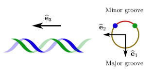
Figure 1: DNA can be represented as an inextensible, twistable, elastic rod. Its conformation is described by a local orthonormal frame, associated with every point along the molecule. $\mathbf{\widehat{e}}_{3}$ is the unit tangent vector, whereas $\mathbf{\widehat{e}}_{1}$ is chosen to lie on the symmetry plane of the grooves. The third vector is given by $\mathbf{\widehat{e}}_{2}=\mathbf{\widehat{e}}_{3}\times\mathbf{\widehat{e}}_{1}$.

Any local deformation of the curve induces a rotation of the frame $\{\mathbf{\widehat{e}}_{1},\mathbf{\widehat{e}}_{2},\mathbf{\widehat{e}}_{3}\}$ from $s$ to $s+ds$, which can be described by the following differential equation

$$\frac{\mathrm{d}\mathbf{\widehat{e}}_{\mu}}{\mathrm{d}s}=(\mathbf{\Omega}+\omega_{0}\mathbf{\widehat{e}}_{3})\times\mathbf{\widehat{e}}_{\mu},$$ (1)

where $\mu=1,2,3$, and $\omega_{0}$ is the intrinsic twist density of the DNA double helix. The vector $\mathbf{\Omega}+\omega_{0}\mathbf{\widehat{e}}_{3}$ is parallel to the axis of rotation from $\mathbf{\widehat{e}}_{\mu}(s)$ to $\mathbf{\widehat{e}}_{\mu}(s+ds)$. Note that in general $\mathbf{\Omega}(s)$ depends on the coordinate $s$. Decomposing this vector along the local frame, we define its three components as $\Omega_{\mu}(s)\equiv\mathbf{\Omega}\cdot\mathbf{\widehat{e}}_{\mu}(s)$. The case $\mathbf{\Omega}=|\mathbf{\Omega}|\mathbf{\widehat{e}}_{3}$ corresponds to a pure twist deformation, whereas $\mathbf{\Omega}=|\mathbf{\Omega}|\mathbf{\widehat{e}}_{1}$ and $\mathbf{\Omega}=|\mathbf{\Omega}|\mathbf{\widehat{e}}_{2}$ express bending in the planes defined by $\mathbf{\widehat{e}}_{1}$ and $\mathbf{\widehat{e}}_{2}$, respectively.

The lowest-energy configuration of the system is that of zero mechanical stress $\Omega_{1}=\Omega_{2}=\Omega_{3}=0$, which corresponds to a straight rod with an intrinsic twist angle per unit length equal to $\omega_{0}$. Expanding around this ground state, one obtains the elastic energy to lowest order in the deformation parameters $\Omega_{\mu}$ as

$$\beta E=\frac{1}{2}\int_{0}^{L}\sum_{\mu,\nu=1}^{3}\Omega_{\mu}(s)M_{\mu\nu}\Omega_{\nu}(s)ds,$$ (2)

where $\beta\equiv 1/k_{\mathrm{B}}T$ is the inverse temperature. The $3\times 3$ symmetric matrix $M_{\mu\nu}$, which we refer to as the stiffness matrix, contains the elastic constants. Note that from Eq. (1) the $\Omega$’s have the dimension of inverse length. As the left-hand side of Eq. (2) is dimensionless, the elements of the stiffness matrix have the dimension of length. In this work sequence-dependent effects will be neglected, therefore $\mathbf{M}$ will not depend on $s$.

Marko and Siggia ¹² argued that, due to the asymmetry introduced by the major and minor grooves, the elastic energy of DNA should be invariant only under the transformation $\Omega_{1}\to-\Omega_{1}$. This implies that $\Omega_{2}\Omega_{3}$ is the only cross-term allowed by symmetry, therefore the stiffness matrix in the Marko-Siggia (MS) model becomes

$$\mathbf{M}_{\text{MS}}=\begin{pmatrix}A_{1}&0&0\\[4.0pt] 0&A_{2}&G\\[4.0pt] 0&G&C\end{pmatrix},$$ (3)

where $A_{1}\equiv M_{11}$, $A_{2}\equiv M_{22}$, $C\equiv M_{33}$ and $G\equiv M_{23}=M_{32}$. $A_{1}$ and $A_{2}$ express the energetic cost of a bending deformation about the local axes $\mathbf{\hat{e}}_{1}$ and $\mathbf{\hat{e}}_{2}$, respectively ¹⁷. $C$ is the intrinsic torsional stiffness, whereas $G$ quantifies the twist-bend coupling interaction. Note that $G\neq 0$ is a direct consequence of the groove asymmetry in the DNA double helix. If one neglects this asymmetry, the MS model reduces to the TWLC model ($G=0$), and the corresponding stiffness matrix becomes diagonal ¹²

$$\mathbf{M}_{\text{TWLC}}=\begin{pmatrix}A_{1}&0&0\\[4.0pt] 0&A_{2}&0\\[4.0pt] 0&0&C\end{pmatrix}.$$ (4)

Most studies ⁵ model DNA as an isotropic TWLC, for which $A_{1}=A_{2}$.

2.2 Computer simulations with oxDNA

In this paper we investigate the elastic properties of oxDNA, which is a model for coarse-grained computer simulations of both single- and double-stranded DNA ¹⁵. The model describes double-stranded DNA as two intertwined strings of rigid nucleotides, with pairwise interactions modeling the backbone covalent bonds, the hydrogen bonding, the stacking, cross-stacking and excluded-volume interactions. oxDNA has been used in the past for the study of a variety of DNA properties ^{15, 18, 16, 19}.

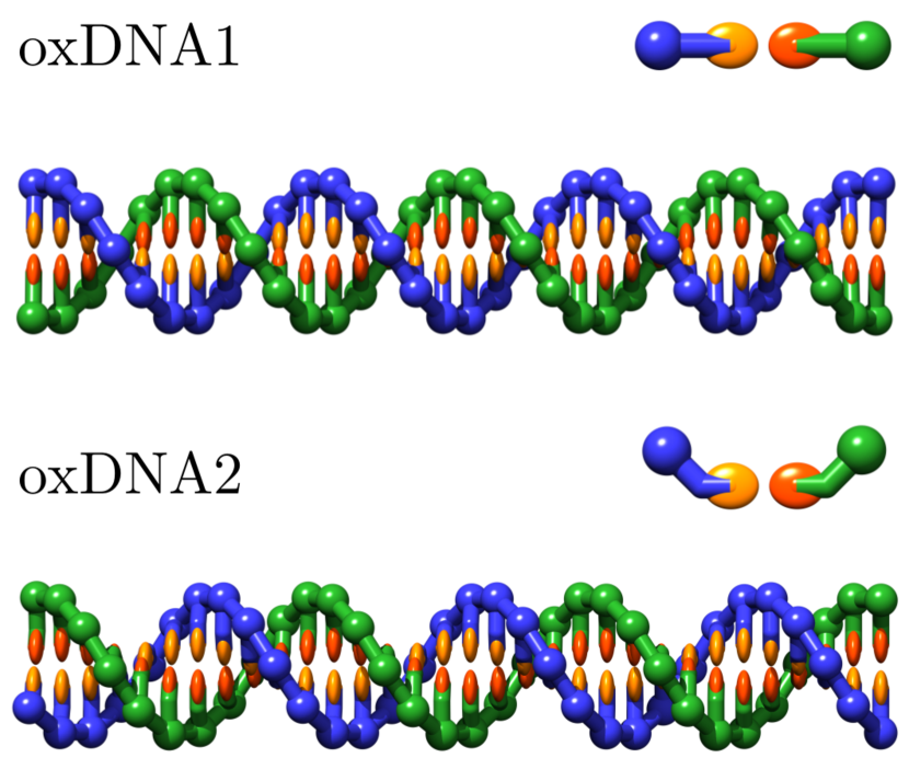
Figure 2: Snapshots of configurations of oxDNA1 (top) and oxDNA2 (bottom), including a cross-section view of the helix. While the grooves are symmetric in oxDNA1, distinct major and minor grooves are present in oxDNA2.

We performed simulations using two available versions of the model. The first version (oxDNA1) describes DNA as a molecule with no distinction between major and minor grooves ¹⁸, while the second (oxDNA2) introduces distinct grooving asymmetry ¹⁶. Figure 2 illustrates molecular conformations of the two models, including a cross-sectional view of a single base pair. As discussed above, the presence of distinct major and minor grooves breaks a molecular symmetry, so we expect that oxDNA1 and oxDNA2 will be mapped onto the TWLC (Eq. (4)) and the MS model (Eq. (3)), respectively.

To sample equilibrium fluctuations, molecular dynamics simulations in the NVE ensemble with an Anderson-like thermostat were used. This is implemented in repeated cycles in which the system is first evolved by integrating Newton’s equations of motion in time for a given number of steps. Then the momenta of some randomly selected particles are chosen from a Maxwell distribution with a desired simulation temperature ($T=295$ K in our case). The cycle then repeats itself a large number of times.

Molecular dynamics simulations were performed on 150 base pair molecules using averaged base pair interaction coefficients. A total of $5\times 10^{10}$ time steps were sampled using a numerical integration time step of $15.2$ fs, and the trajectories were recorded every $5\times 10^{4}$ time steps. For all simulations the salt concentration was set to $0.5$ M. In oxDNA1 this value is fixed, since the electrostatic interactions are implemented through excluded-volume potentials, parametrized to mimic high salt concentration (i.e. $0.5$ M). oxDNA2 improved upon this approach by switching to a Debye-Hückel potential, which models the ionic screening of electrostatic interactions. This allows for the explicit selection of a salt concentration, which we set to $0.5$ M, in order to achieve optimal comparability between the two models.

2.3 Extraction of elastic parameters

The pivotal objective of the extraction of elastic parameters is to map oxDNA onto the described elastic model in such a way, that both the elastic properties at the base pair level as well as long range behavior, such as bending and torsional persistence lengths, are captured as accurately as possible. Establishing an appropriate one-to-one correspondence requires the reduction of both models to the same level of complexity. For the continuous elastic model this implies the discretization of the elastic free energy functional Eq. (2) to the base pair level

$$\beta E = \frac{a}{2}\sum_{n=1}^{N}\left(\sum_{\mu,\nu=1}^{3}\Omega_{\mu}^{(n)}M_{\mu\nu}\Omega_{\nu}^{(n)}\right),$$ (5)

where $a=0.34$ nm is the mean distance between successive base pairs and $\Omega_{\mu}^{(n)}\equiv\Omega_{\mu}(na)$. In the discrete case the finite rotation of a local frame of reference (triad) $\{\mathbf{\widehat{e}}_{1}(n),\mathbf{\widehat{e}}_{2}(n),\mathbf{\widehat{e}}_{3}(n)\}$, associated with the spatial orientation of the $n$-th base pair of the molecule, into the sequentially adjacent triad $\{\mathbf{\widehat{e}}_{1}(n+1),\mathbf{\widehat{e}}_{2}(n+1),\mathbf{\widehat{e}}_{3}(n+1)\}$, can be represented by a rotation vector $\mathbf{\Theta}^{(n)}$. The deformation parameters $\Omega_{\mu}^{(n)}$ can then be defined as the deviations of the components of $\mathbf{\Theta}^{(n)}/a$ from their respective mean values

$$a\Omega_{\mu}^{(n)}\equiv\Theta_{\mu}^{(n)}-\left\langle\Theta_{\mu}^{(n)}\right\rangle.$$ (6)

For oxDNA1 the mean twist angle $a\omega_{0}=\langle\Theta_{3}^{(n)}\rangle$ is found to be $34.8^{\circ}$, whereas for oxDNA2 we find $34.1^{\circ}$.

Accordingly, an appropriate triad has to be assigned to each base pair of the oxDNA model. The particular choice of those triads contains a certain degree of ambiguity, resulting in different mappings for different triads. Such an ambiguity regarding the definition of the tangent vector $\mathbf{\widehat{e}}_{3}$ in coarse-grained simulations of DNA and the related implications for the extraction of the bending persistence length have for instance been discussed by Fathizadeh et al. ²⁰, who showed that, when considering short length scales, different definitions of the local tangent vector will usually yield significantly different results for the bending persistence length. However, when considering longer length scales, i.e. comparing more distant tangent vectors, those discrepancies vanish asymptotically.
For a detailed discussion of different triad definitions we refer to the Supplementary Material. All results presented in the main text are calculated with a triad definition employing local tangents $\mathbf{\widehat{e}}_{3}$ obtained from the mean vector of the intrinsic orientation of the two nucleotides in each basepair, provided by the oxDNA output. The unit vector $\mathbf{\widehat{e}}_{2}$ is obtained from the projection of the connecting vector between the centers of the two nucleotides $\mathbf{y}$, onto the orthogonal space of $\mathbf{\widehat{e}}_{3}$. Having identified $\mathbf{\widehat{e}}_{3}$ and $\mathbf{\widehat{e}}_{2}$ the remaining vector in the right-handed triad is now uniquely defined as $\mathbf{\widehat{e}}_{1}=\mathbf{\widehat{e}}_{2}\times\mathbf{\widehat{e}}_{3}$. This corresponds to Triad II in the Supplementary Material.

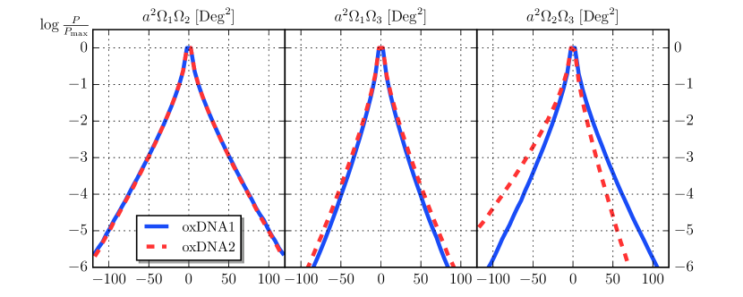
Figure 3: Histograms of cross-diagonal terms $\Omega_{\mu}\Omega_{\nu}$ for oxDNA1 and oxDNA2. The histograms for $\Omega_{1}\Omega_{2}$ and $\Omega_{1}\Omega_{3}$ are quite similar for the two models, while there is a marked difference for $\Omega_{2}\Omega_{3}$. The asymmetric shape of the histogram in oxDNA2 is a signature of the presence of twist-bend coupling.

In order to infer the stiffness matrix from simulations, we used the standard procedure (see e.g. Ref. 13) which relies on the equipartition theorem ²¹

$$\left\langle\Omega_{\mu}^{(n)}\,\frac{\partial\beta E}{\partial\Omega_{\nu}^{(n)}}\right\rangle=\delta_{\mu\nu},$$ (7)

where $\langle\cdot\rangle$ indicates the thermal average. Then we introduced the $3\times 3$ covariance matrix with elements

$$\Lambda_{\mu\nu}\equiv\left\langle\Omega_{\mu}^{(n)}\,\Omega_{\nu}^{(n)}\right\rangle,$$ (8)

where the index $n$ was dropped from $\Lambda$, as we neglect sequence-dependent effects. Combining (5) and (7) we get

$$\mathbf{M}=\frac{1}{a}\mathbf{\Lambda}^{-1}.$$ (9)

Thus, the stiffness parameters contained in $\mathbf{M}$ can be extracted from the correlation matrix $\mathbf{\Lambda}$, obtained from equilibrium fluctuations (Eq. (8)).

This procedure is based on the elastic energy being given by Eq. (5), which in turn assumes that there are no correlations between different sets of $\Omega$’s. To investigate the effect of correlations we introduce the matrix

$$\Xi_{\mu\nu}(m)\equiv\left\langle\left[\sum_{k=n}^{n+m-1}\Omega_{\mu}^{(k)}\right]\left[\sum_{l=n}^{n+m-1}\Omega_{\nu}^{(l)}\right]\right\rangle.$$ (10)

If correlations beyond neighboring bases are weak, the cross-terms in the previous expression can be neglected and we obtain

$$\Xi_{\mu\nu}(m)\approx\sum_{k=n}^{n+m-1}\left\langle\Omega_{\mu}^{(k)}\Omega_{\nu}^{(k)}\right\rangle=m\Lambda_{\mu\nu}.$$ (11)

Finally we define the $m$-step stiffness matrix as

$$\mathbf{M}(m)\equiv\frac{m}{a}\left[\mathbf{\Xi}(m)\right]^{-1},$$ (12)

from which the $m$-step elastic constants can be obtained. In absence of correlations, this matrix will not depend on $m$.

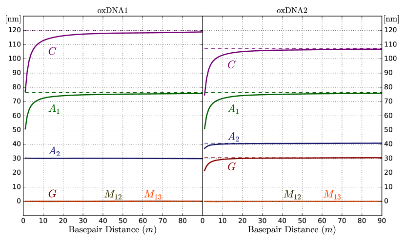
Figure 4: Elastic parameters, obtained from the $m$-step stiffness matrix, as a function of the base pair distance $m$. The remarkable difference between these two sets is the appearance of a significant twist-bend coupling term $G$ for oxDNA2, in contrast to its negligible value in oxDNA1. This is in agreement with the original prediction of Marko and Siggia ¹².

3 Results

We present here the results of the simulations highlighting the differences in elastic properties between oxDNA1 and oxDNA2.

Probability Distributions

Qualitative evidence of the presence of a non-zero twist-bend coupling in the energy functionals can already be inferred from the distribution of the off-diagonal terms $\Omega_{\mu}^{(n)}\Omega_{\nu}^{(n)}$ with $\mu\neq\nu$. Figure 3 shows histograms of these quantities, obtained from simulations of oxDNA1 and oxDNA2. The data are averaged over all base pairs along the DNA contour, hence we drop the position index $n$. While the distribution of $\Omega_{1}\Omega_{2}$ and $\Omega_{1}\Omega_{3}$ is symmetric and very similar in oxDNA1 and oxDNA2, there is a marked difference between the two models in the histogram of $\Omega_{2}\Omega_{3}$. In oxDNA1 the distribution appears to be symmetric, whereas in oxDNA2 there is a clear asymmetry, suggesting the existence of a coupling between those deformation parameters.

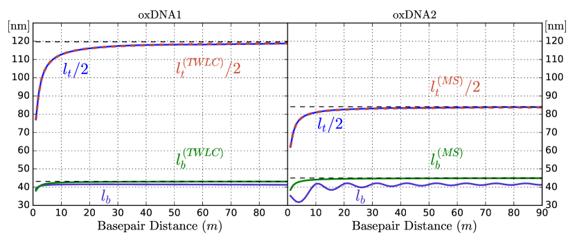
Figure 5: Blue lines: plots of $l_{\text{b}}$ and $l_{\text{t}}/2$ obtained from oxDNA simulations using Eqs. (14) and (15). Orange and green lines: analytical predictions for the same quantities in the TWLC (Eqs. (16) and (17)) and in the MS model (Eqs. ((18) and (19)), where the $m$-dependent stiffnesses of Fig. 4 were used.The values obtained from the plateau values of the elastic parameters are indicated by the dashed black lines.

Stiffness Matrix

In order to quantify the observed twist-bend coupling interaction, we computed the $m$-step stiffness matrix $\mathbf{M}(m)$, as defined in Eq. (12), for both models and for different summation lengths $m$. At both chain-ends 5 base pairs were excluded from this calculation, since those boundary segments are found to exhibit a significantly higher flexibility than segments located in the center of the chain. The results are shown in Fig. 4, where the elements of $\mathbf{M}(m)$ are plotted as a function of $m$. In both models the diagonal elements $A_{1}$, $A_{2}$ and $C$, as defined in Eqs. (3) and (4), have distinct, non-vanishing values. There is, however, a remarkable difference between oxDNA1 and oxDNA2 in the values of the off-diagonal elements $G$, $M_{12}$ and $M_{13}$. In particular, all off-diagonal elements in oxDNA1 are orders of magnitude smaller than the diagonal ones. On the other hand, although $M_{12}$ and $M_{13}$ remain negligibly small, the twist-bend coupling $G$ in oxDNA2 becomes comparable in magnitude to the diagonal terms, which clearly has to be attributed to the asymmetry of the helical grooves. These results are in line with the predictions of Marko and Siggia ¹² and remain valid regardless of the exact choice of coordinate systems (see Supplementary Material).

Table 1: Values of the stiffness coefficients for oxDNA1 and oxDNA2 obtained in this work (expressed in nm). The last line shows the values obtained from fitting the MS model to magnetic tweezers data.

	$A_{1}$	$A_{2}$	C	G
oxDNA1	84(14)	29(2)	118(1)	0.1(0.2)
oxDNA2	81(10)	39(2)	105(1)	30(1)
Nomidis et al. 11	66	46	110(5)	40(10)

As discussed in the previous section, in absence of correlations between different sets of $\Omega$’s, the elements of $\mathbf{M}(m)$ are expected to be independent of $m$. The results of Fig. 4, however, show that this is not exactly true, which is a signature of the influence of correlations between base pairs separated by more than one nucleotide (though the convergence to a limiting value for increasing $m$ is quite rapid).

When comparing the results among different choices of frames, we find that, despite the different values for $m=1$, at large $m$ all values are close to each other (see Supplementary Material). We, thus, consider these limiting values to be good estimates for the stiffness parameters of the elastic model, onto which oxDNA is mapped. Table 1 summarizes the estimated values of the elastic parameters, averaged over the different choices of local frames, where the error bars reflect the uncertainty from estimates obtained from four different definitions of frames. The first two rows in Table 1 are data obtained from oxDNA simulations in this work, while the last row shows the parametrization obtained from fits of the MS model to magnetic tweezers data ¹¹. oxDNA2 data for $C$ and $G$ are consistent with the latter, while some differences are found in $A_{1}$ and $A_{2}$. It should be noted, however, that the fitting procedure used in Ref. 11 was not very sensitive to the specific choice of $A_{1}$ and $A_{2}$, as other choices fitted the experimental data equally well. The overall quantitative agreement between the oxDNA2 parameters and those from this recent study supports the choice of the plateau values in Fig. 4 as an estimate for the elastic parameters.

The value obtained for $C$ is in general good agreement with previous estimates for oxDNA, which were obtained from methods not involving the calculation of the stiffness matrix. From two independent measurements ^{22, 23} the value $C=115$ nm was reported for oxDNA1. In oxDNA2 a fit of torsional stiffness data ¹⁶ gives $C=93-98$ nm, which is slightly lower than our current estimate.

Persistence lengths

Any twistable polymer model is characterized by two distinct persistence lengths, related to bending and twisting fluctuations. The bending persistence length can be obtained from the decay of the correlation between tangent vectors

$$\left\langle\mathbf{\widehat{e}}_{3}(n)\cdot\mathbf{\widehat{e}}_{3}(n+m)\right\rangle\equiv\langle\cos\theta(m)\rangle\sim e^{-ma/l_{\text{b}}},$$ (13)

where $\theta(m)$ is the angle formed by the two vectors. As the exponential decay is valid asymptotically in $m$, we can estimate the bending persistence length from the extrapolation at large $m$ of the quantity

$$l_{\text{b}}(m)\equiv-\frac{ma}{\log\left\langle\cos\theta(m)\right\rangle}.$$ (14)

Analogously, we can define the twisting persistence length from the decay of the average twist angle

$$l_{\text{t}}(m)\equiv-\frac{ma}{\log\left\langle\cos\sum_{k=n}^{n+m-1}\Omega_{3}^{(k)}\right\rangle}.$$ (15)

Equations (14) and (15) can be compared to some analytical expressions. In the TWLC the bending persistence length $l_{\text{b}}$ is the harmonic mean of the two bending stiffnesses ^{24, 25}:

$$l_{\text{b}}=\frac{2A_{1}A_{2}}{A_{1}+A_{2}}$$ (16)

while the twist persistence length is just twice the torsional stiffness (see e.g. Ref. 26)

$$l_{\text{t}}=2C.$$ (17)

The same quantities have been calculated for the MS model ¹¹

$$l_{\text{b}}=2A_{1}\frac{A_{2}-G^{2}/C}{A_{1}+A_{2}-G^{2}/C}$$ (18)

and

$$l_{\text{t}}=2C\left(1-\frac{G^{2}}{A_{2}C}\right).$$ (19)

From the last two expressions one recovers the TWLC limit upon setting $G=0$.

Table 2: Elements of the stiffness matrix (expressed in nm) for different base pairs, obtained from all-atom simulations (courtesy of F. Lankaš and T. Dršata). In order to facilitate the readout, we have included the tilt, roll and twist nomenclature, which corresponds to our definition of $\Omega_{1}$, $\Omega_{2}$ and $\Omega_{3}$, respectively.

		CG	CA	TA	AG	GG	AA	GA	AT	AC	GC	average
$A_{1}$	(tilt-tilt)	47.6	50.6	44.5	67.3	70.7	60.9	69.9	73.6	75.0	70.0	63.0
$A_{2}$	(roll-roll)	27.7	31.4	24.5	41.0	44.4	42.2	38.7	45.1	46.1	47.3	38.8
$C$	(twist-twist)	32.7	34.0	57.6	57.9	58.9	49.5	46.6	77.7	65.1	51.7	53.2
$G$	(roll-twist)	3.7	5.8	14.1	6.7	7.4	10.5	15.7	11.9	13.4	13.0	10.2
$M_{12}$	(tilt-roll)	2.8	1.3	0.1	-5.3	-1.7	3.6	-0.2	0.4	4.0	-0.5	0.4
$M_{13}$	(tilt-twist)	4.4	-1.5	-1.1	-3.9	0.9	6.7	0.0	-0.7	-0.6	-0.7	0.4

Figure 5 shows a comparison of the persistence lengths, as obtained from Eq. (14) and (15), with the analytical expressions of the TWLC (Eqs. (16) and (17)) and the MS model (Eqs. (18) and (19)). There is a good overall agreement between the direct computation of the persistence lengths and Eqs. (18) and (19) (with the plateau values of Fig. 4), for both oxDNA1 and oxDNA2. In particular, the prediction of the twisting persistence length is excellent in both models, whereas some small deviations are observed for $l_{\text{b}}$ (smaller than 10 %). This suggests that there are some features of oxDNA which are not fully captured by the “projection” to an inextensible elastic model, as described by Eq. (2). Note that $l_{\text{b}}$ in oxDNA2 exhibits a damped oscillatory behaviour at short lengths $m$ with the helix periodicity, suggesting that the tangent vectors are systematically misaligned. The value of the bending persistence length calculated here is in agreement with previous published oxDNA1 and oxDNA2 data ^{22, 23, 16}.

4 Discussion

Owing to its chirality, DNA has been found to possess some remarkable mechanical properties, such as twist-bend ¹² and twist-stretch coupling ²⁷. Although the latter has been investigated in several studies ^{28, 29, 30, 31, 32}, the effect of twist-bend coupling remains to date largely unexplored. Motivated by some recently resurgent interest ¹¹, we have investigated the origin of this interaction in oxDNA, a coarse-grained model of nucleic acids. Twist-bend coupling is a cross-interaction between twist and bending degrees of freedom. In the context of DNA, the existence of such an interaction was predicted by Marko and Siggia ¹², who argued that twist-bend coupling follows from the groove asymmetry, a characteristic of the DNA molecular structure.

OxDNA is particularly suited to investigate the origin of twist-bend coupling, as it comes in two different versions (oxDNA1 and oxDNA2). The double helical grooves are symmetric in oxDNA1 and asymmetric in oxDNA2, with widths reproducing the average B-DNA geometry. Our simulations, sampling equilibrium conformations of both oxDNA1 and oxDNA2, show that only the latter model has a significant twist-bend coupling term (Fig. 4). This is in agreement with the symmetry argument by Marko and Siggia ¹².

The estimated twist-bend coupling coefficient from oxDNA2 is $G=30\pm 1$ nm, which agrees with the value $G=40\pm 10$ nm, obtained from fitting magnetic tweezers data ¹¹. An earlier estimate of $G\approx 25$ nm was obtained from the analysis of structural correlations of DNA wrapped around histone proteins ¹⁴. It is worth noting that all-atom simulations also support the existence of a twist-bend coupling term ^{13, 24, 33}, although those studies are restricted to short fragments ($\approx 20$ bp). Table 2 contains the elements of one-step stiffness matrices, obtained by Lankaš et al. ²⁴ from all-atom simulations.

Although the original analysis included various stretching deformations, here we only show the rotational coordinates, while the translational degrees of freedom are integrated out. The data in Table 2 refer to deformations between neighboring base pairs, hence they are the counterparts of the $m=1$ data of Fig. 4 and cannot be used as reliable estimates of asymptotic values of the elastic parameters. Nonetheless, the averages over all possible sequence combinations (last column of Table 2) show that twist-bend coupling is much larger than the other off-diagonal terms, i.e. $G\gg M_{12},M_{13}$.

One of the most remarkable effects of twist-bend coupling in DNA is the appearance of a novel twist length scale ¹¹ (Eq. (19)) with an associated twist stiffness $\kappa_{\text{t}}=l_{\text{t}}/2$, which differs from the intrinsic value $C$. We refer to $\kappa_{\text{t}}$ as the renormalized twist stiffness. In the MS and TWLC models a pure twist deformation ($\Omega_{1}=\Omega_{2}=0$, $\Omega_{3}\neq 0$) has an associated intrinsic stiffness $C$. In the presence of bending fluctuations ($\langle\Omega_{1}^{2}\rangle$, $\langle\Omega_{2}^{2}\rangle>0$), however, the two models behave differently. While the torsional stiffness of the TWLC remains the same, in the MS model twist deformations are governed by a lower stiffness $\kappa_{\text{t}}<C$. In other words, in the presence of bending fluctuations, twist-bend coupling makes the DNA molecule torsionally softer. From oxDNA2 simulations we estimate $\kappa_{\text{t}}=l_{\text{t}}/2\approx 83$ nm (see Fig. 5). This is close to the value $\kappa_{\text{t}}=75$ nm, recently obtained from fitting the MS model to magnetic tweezers data ¹¹. The above effect naturally explains ¹¹ some reported discrepancies in the experimental determination of $C$.

Having shown that the twist-bend coupling is a relevant interaction in DNA, one can ask in which limits and for which quantities the TWLC can still be considered a good DNA model. Our work shows that one can map freely fluctuating DNA onto a TWLC using $C\approx 80$ nm as twist elastic parameter, which incorporates the effect of twist-bend coupling. However some care needs to be taken in the presence of a stretching force, as the suppression of bending fluctuation will influence the twist stiffness. At high forces DNA will then be mapped onto an effective TWLC with a higher value of $C$. Finally, it will be important to investigate the effect of twist-bend coupling in cases where DNA behavior is influenced by its mechanics as in DNA supercoiling ^{34, 35} or in DNA-protein interactions ^{36, 37}.

5 Supplementary Material

In the Supplementary Material the different triads are defined and the corresponding stiffness parameters are presented. Furthermore we elaborate on how to obtain the rotation vector $\mathbf{\Omega}$ from subsequent triads. Moreover, we explored sequence-dependent effects, by investigating some specific sequences with oxDNA. Finally, we extended the analysis of the main text to oxRNA.

Discussions with F. Kriegel, F. Lankaš, J. Lipfert, C. Matek and W. Vanderlinden are gratefully acknowledged. We thank T. Dršata for analyzing the all-atom simulation trajectories ²⁴, from which stiffness data in Table 2 were obtained. We acknowledge financial support from KU Leuven grant IDO/12/08, and from the Research Funds Flanders (FWO Vlaanderen) grant VITO-FWO 11.59.71.7N

Supporting Information for “DNA elasticity from coarse-grained simulations: the effect of groove asymmetry"

This document contains additional information and results in support of the main manuscript.

Triad Definitions

Continuous Chain

In order to describe any local deformations of an inextensible, elastic rod, onto which DNA can be mapped, one has to introduce a local frame of reference $\{\mathbf{\widehat{e}}_{1}(s),\mathbf{\widehat{e}}_{2}(s),\mathbf{\widehat{e}}_{3}(s)\}$ (triad) to every point along the rod. The deformations can thus be determined from the rotation of one triad into the next one. In the case of a continuous chain, the following differential equation will hold

$$\frac{\mathrm{d}\mathbf{\widehat{e}}_{\mu}}{\mathrm{d}s}=(\mathbf{\Omega}+\omega_{0}\mathbf{\widehat{e}}_{3})\times\mathbf{\widehat{e}}_{\mu}$$ (20)

and this frame of reference can be unambiguously defined: $\mathbf{\widehat{e}}_{3}$ may be taken to be the tangent to the curve, $\mathbf{\widehat{e}}_{1}$ pointing along the symmetry axis of the two grooves (oriented towards the major groove) and $\mathbf{\widehat{e}}_{2}$ simply given by $\mathbf{\widehat{e}}_{2}=\mathbf{\widehat{e}}_{3}\times\mathbf{\widehat{e}}_{1}$.

oxDNA

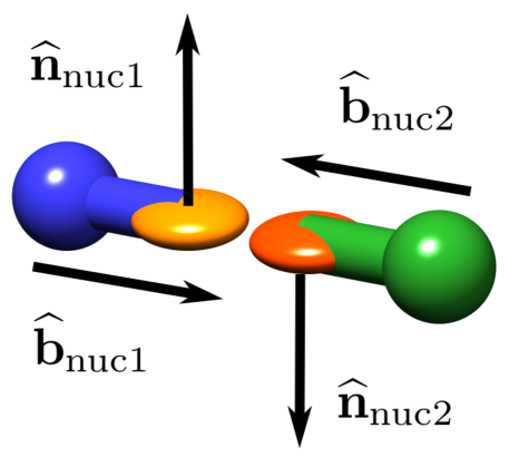
Figure 6: Besides the center-of-mass position, oxDNA stores two vectors for each nucleotide. A unit vector $\mathbf{\widehat{b}}$ connects the backbone with the base, and a normal vector $\mathbf{\widehat{n}}$ defines the plane of the base. The blue and green spheres represent the backbone sites, whereas the yellow and orange ones correspond to the base planes.

In the discrete case of oxDNA, different triads can be defined using the few reference points provided by the coarse-grained model. In particular, oxDNA consists of rigid nucleotides represented by three interactions sites: the hydrogen-bonding, stacking and backbone sites (T. Ouldridge, PhD Thesis, University of Oxford (2011)). The orientation of each nucleotide is given by a normal vector $\mathbf{\widehat{n}}$, specifying the plane of the base, and a vector $\mathbf{\widehat{b}}$ pointing from the stacking site to the hydrogen-bonding site (as in Fig. 6). For oxDNA1 all three sites lie on the same straight line, while in oxDNA2 the position of the backbone site is changed, thus inducing the grooving asymmetry (B.E. Snodin et al. J. Chem. Phys. 142, 234901 (2015)). Hence each base-pair comes with 2 intrinsic triads (one per nucleotide), with the normal vectors pointing in the respective 5’-3’ direction of the strands. The interactions are designed such that in the minimum energy configuration the vectors $\mathbf{\widehat{b}}_{\text{nuc1}}$ and $\mathbf{\widehat{b}}_{\text{nuc2}}$, attached to the two nucleotides of the same base-pair, point directly towards each other.

In what follows we present the four different choices of triads we have tested.

Triad I.

The aforementioned intrinsic nucleotide triads present a natural definition for the triad attached to a base pair. The base-pair normal vector can be constructed as the average vector of the nucleotide normal vectors

$$\mathbf{\widehat{e}}_{3}=\frac{\mathbf{\widehat{n}}_{\text{nuc1}}-\mathbf{\widehat{n}}_{\text{nuc2}}}{\left\lVert\mathbf{\widehat{n}}_{\text{nuc1}}-\mathbf{\widehat{n}}_{\text{nuc2}}\right\rVert}.$$ (21)

The mean vector of $\mathbf{\widehat{b}}_{\text{nuc1}}$ and $\mathbf{\widehat{b}}_{\text{nuc2}}$

$$\mathbf{\widehat{y}}=\frac{\mathbf{\widehat{b}}_{\text{nuc1}}-\mathbf{\widehat{b}}_{\text{nuc2}}}{\left\lVert\mathbf{\widehat{b}}_{\text{nuc1}}-\mathbf{\widehat{b}}_{\text{nuc2}}\right\rVert}$$ (22)

can be approximately identified with $\mathbf{\widehat{e}}_{2}$, however in general it will fail to be orthogonal to $\mathbf{\widehat{e}}_{3}$. This can easily be rectified by projecting it onto the orthogonal space of $\mathbf{\widehat{e}}_{3}$

$$\mathbf{\widehat{e}}_{2}=\frac{\mathbf{\widehat{y}}-(\mathbf{\widehat{y}}\cdot{\mathbf{\widehat{e}}_{3})\mathbf{\widehat{e}}_{3}}}{\left\lVert\mathbf{\widehat{y}}-(\mathbf{\widehat{y}}\cdot{\mathbf{\widehat{e}}_{3})\mathbf{\widehat{e}}_{3}}\right\rVert}.$$ (23)

The last vector is simply given by $\mathbf{\widehat{e}}_{1}=\mathbf{\widehat{e}}_{2}\times\mathbf{\widehat{e}}_{3}$.

Triad II.

Alternatively, $\mathbf{\widehat{e}}_{2}$ can be obtained from connecting the centers of mass $\mathbf{r}_{\text{nuc1}}$ and $\mathbf{r}_{\text{nuc2}}$ of the two nucleotides

$$\mathbf{\widehat{y}}=\frac{\mathbf{r}_{\text{nuc1}}-\mathbf{r}_{\text{nuc2}}}{\left\lVert\mathbf{r}_{\text{nuc1}}-\mathbf{r}_{\text{nuc2}}\right\rVert}$$ (24)

and the complete triad can be found in a completely analogous way as for Triad I. This particular choice of triad was used in the main article, as it appeared to be the most robust (i.e. it yielded the smallest correlations between consecutive $\Omega_{\mu}$).

Triad III.

The tangent vector can also be constructed using the center of mass of the nucleotides. The center of mass of the i-th basepair can be defined as

$$\mathbf{R_{\text{bp}}}(i)=\frac{\mathbf{r}_{\text{nuc1}}(i)+\mathbf{r}_{\text{nuc2}}(i)}{2}.$$ (25)

Identifying the normalized connectors of consecutive $\mathbf{R_{\text{bp}}}(i)$ with $\mathbf{\widehat{e}}_{3}$ would result in a directionally-dependent definition, therefore $\mathbf{\widehat{e}}_{3}$ was chosen as the connector between the center of masses of the previous and next basepair

$$\mathbf{\widehat{e}}_{3}(i)=\frac{\mathbf{R_{\text{bp}}}(i+1)-\mathbf{R_{\text{bp}}}(i-1)}{\left\lVert\mathbf{R_{\text{bp}}}(i+1)-\mathbf{R_{\text{bp}}}(i-1)\right\rVert}.$$ (26)

The definition of the remaining triad versors is identical to the one used for Triad II.

Triad IV.

Instead of selecting one vector as the arithmetic mean and projecting the others on its orthogonal space, one can attempt to treat them on a more equal footing. By placing the 3 nucleotide triad vectors in the columns of a matrix one obtains a rotation matrix

$$\mathbf{T}_{\text{nuc}}=[\mathbf{\widehat{t}}_{\text{nuc}},\mathbf{\widehat{b}}_{\text{nuc}},\mathbf{\widehat{n}}_{\text{nuc}}]\in SO(3),$$ (27)

with $\mathbf{\widehat{t}}_{\text{nuc}}=\mathbf{\widehat{b}}_{\text{nuc}}\times\mathbf{\widehat{n}}_{\text{nuc}}$. The arithmetic mean $\overline{\mathbf{T}}=\frac{1}{2}\left(\mathbf{T}_{\text{nuc1}}+\mathbf{T}_{\text{nuc2}}\right)$ will generally not be a rotation matrix itself, it is however possible to orthogonally project $\overline{\mathbf{T}}$ onto $SO(3)$. It can be shown that this projection is given by (M. Moakher, SIAM J. Matrix Anal. Appl. 24, 1 (2002))

$$\mathbf{T}=\overline{\mathbf{T}}\mathbf{U}\;\text{diag}\left(\frac{1}{\sqrt{\Lambda_{1}}}\text{,}\frac{1}{\sqrt{\Lambda_{2}}}\text{,}\frac{s}{\sqrt{\Lambda_{3}}}\right)\mathbf{U}^{\intercal},$$ (28)

where $\overline{\mathbf{T}}=\frac{1}{N}\sum_{k=1}^{N}T^{(k)}$, $\Lambda_{1}\geq\Lambda_{2}\geq\Lambda_{3}\geq 0$ are the eigenvalues of $\mathbf{M}=\overline{\mathbf{T}}^{\intercal}\overline{\mathbf{T}}$ and the matrix $\mathbf{U}$ is defined so that $\mathbf{U}^{\intercal}\mathbf{M}\mathbf{U}=\text{diag}(\Lambda_{1},\Lambda_{2},\Lambda_{3})$. The variable $s$ satisfies $s=1$ if $\det\overline{\mathbf{T}}>0$ and $s=-1$ if $\det\overline{\mathbf{T}}<0$.

Calculation of $\Omega$

Eq. (20) (valid for infinitesimal rotations) can be generalized for finite rotations. According to Rodrigues’ rotation formula, the rotation of a vector $\mathbf{v}$ about an axis $\mathbf{\widehat{\Theta}}$ by an angle $\Theta$ is given by

$$\mathbf{v}_{\text{rotated}} = \mathbf{v}\cos\Theta+\left(\mathbf{\widehat{\Theta}}\times\mathbf{v}\right)\sin\Theta+$$ (29)

$$\mathbf{\widehat{\Theta}}\left(\mathbf{\widehat{\Theta}}\cdot\mathbf{v}\right)\left(1-\cos\Theta\right).$$

From each triad one can construct an orthogonal matrix, by placing the triad vectors in the columns of a $3\times 3$ matrix

$$\mathbf{T}(i)=[\mathbf{\widehat{e}}_{1}(n),\mathbf{\widehat{e}}_{2}(n),\mathbf{\widehat{e}}_{3}(n)]\in SO(3).$$ (30)

This matrix is exactly the rotation matrix, transforming the canonical frame into the frame of the respective triad. The matrix rotating $\mathbf{T}(n)$ into $\mathbf{T}(n+1)$ with respect to the coordinate system of the $n$-th triad is given by

$$\mathbf{R}=\mathbf{T}^{\intercal}(n)\mathbf{T}(n+1).$$ (31)

It is straightforward to show that in this frame the rotation matrix $\mathbf{R}$ can by written in terms of the components of the rotation vector $\mathbf{\Theta}=\left(\Theta_{1}\;\Theta_{2}\;\Theta_{3}\right)^{\intercal}$

$$\mathbf{R}(\mathbf{\Theta})=\begin{pmatrix}\cos\Theta+\left(\frac{\Theta_{1}}{\Theta}\right)^{2}\left(1-\cos\Theta\right)&\frac{\Theta_{1}\Theta_{2}}{\Theta^{2}}\left(1-\cos\Theta\right)-\frac{\Theta_{3}}{\Theta}\sin\Theta&\frac{\Theta_{1}\Theta_{3}}{\Theta^{2}}\left(1-\cos\Theta\right)+\frac{\Theta_{2}}{\Theta}\sin\Theta\\[4.0pt] \frac{\Theta_{1}\Theta_{2}}{\Theta^{2}}\left(1-\cos\Theta\right)+\frac{\Theta_{3}}{\Theta}\sin\Theta&\cos\Theta+\left(\frac{\Theta_{2}}{\Theta}\right)^{2}\left(1-\cos\Theta\right)&\frac{\Theta_{2}\Theta_{3}}{\Theta^{2}}\left(1-\cos\Theta\right)-\frac{\Theta_{1}}{\Theta}\sin\Theta\par\\[4.0pt] \frac{\Theta_{1}\Theta_{3}}{\Theta^{2}}\left(1-\cos\Theta\right)-\frac{\Theta_{2}}{\Theta}\sin\Theta&\frac{\Theta_{2}\Theta_{3}}{\Theta^{2}}\left(1-\cos\Theta\right)+\frac{\Theta_{1}}{\Theta}\sin\Theta&\cos\Theta+\left(\frac{\Theta_{3}}{\Theta}\right)^{2}\left(1-\cos\Theta\right)\end{pmatrix}.$$ (32)

The components of $\mathbf{\Theta}$ can now be extracted by equating Eqs. (31) and (32) and solving for $\Theta_{1}$, $\Theta_{2}$ and $\Theta_{3}$. A simple way to do this is by noticing that

$$\text{tr}(\mathbf{R})=1+2\cos\Theta.$$ (33)

Moreover, one can also verify that the following relation holds

$$\mathbf{\Theta}=\frac{\Theta}{2\sin\Theta}\begin{pmatrix}R_{32}-R_{23}\\[4.0pt] R_{13}-R_{31}\\[4.0pt] R_{21}-R_{12}\end{pmatrix}.$$ (34)

Note that the sign ambiguity presented in Eq. (33) is completely inconsequential for Eq. (34).

We define the deformation parameters $\Omega_{\mu}$ as the deviations of the components of $\mathbf{\Theta}/a$ from their respective mean value

$$a\Omega_{\mu}\equiv\Theta_{\mu}-\left\langle\Theta_{\mu}\right\rangle.$$ (35)

For an ideal triad definition, the mean values of $\Theta_{1}$ and $\Theta_{2}$ are expected to be zero, while $\left\langle\Theta_{3}\right\rangle/a$ should be equal to the intrinsic twist $\omega_{0}$. In the case of oxDNA2, the mean value of $\Theta_{2}$ is in fact distinctly non-zero (about $2.6^{\circ}$ for Triad II and very similar for the other triads), resulting in the oscillatory behavior of the persistence length shown in Fig. 5 of the main text. All triad definitions consistently yield $\left\langle\Theta_{3}\right\rangle\approx 34.8^{\circ}$ and $\left\langle\Theta_{3}\right\rangle\approx 34.1^{\circ}$ for oxDNA1 and oxDNA2 respectively.

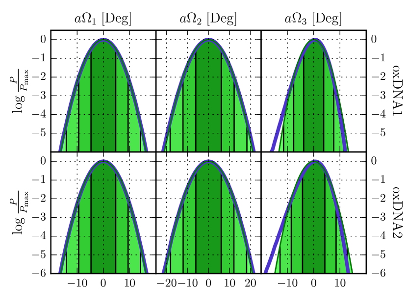
Figure 7: Probability distribution of $\Omega_{\mu}$ for oxDNA1 and oxDNA2 in logscale, using Triad II. The distributions coincide very well with Gaussian distributions, validating the use of a quadratic form for the free energy. Analogous distributions are found for the other choices of triads.

Distributions of $\Omega$’s

The approximation of the free energy by a quadratic form

$$\beta E = \frac{a}{2}\sum_{n=1}^{N}\left(\sum_{\mu,\nu=1}^{3}\Omega_{\mu}^{(n)}M_{\mu\nu}\Omega_{\nu}^{(n)}\right)$$ (36)

implicitly assumes that the deformation parameters follow a Gaussian distribution. Figure 7 shows the distributions of $\Omega_{1}$, $\Omega_{2}$ and $\Omega_{3}$ (blue lines) as obtained from equilibrium simulations. For a clear comparison, the distributions are shown in logarithmic scale. The fitted Gaussian curves (green lines) indicate that the quadratic approximation is excellent for $\Omega_{1}$ and $\Omega_{2}$, while some small deviations are observed in the distributions of $\Omega_{3}$ (noticeable for angles larger than $15$ degrees). The distributions of $\Omega_{3}$ are slightly asymmetric, which is a consequence of the intrinsic twist $\omega_{0}$ (different response of DNA to under- and over-twisting).

Stiffness parameters for alternative triads definitions

The extracted stiffness parameters for the 4 different triads are summarized in Fig. 8 and Table 3. The plateau values (large $m$) are quite consistent among the different triad definitions, with the exception of $A_{1}$ and $A_{2}$ obtained from Triad III. On the other hand, the values obtained for $m=1$ are significantly more diverse.

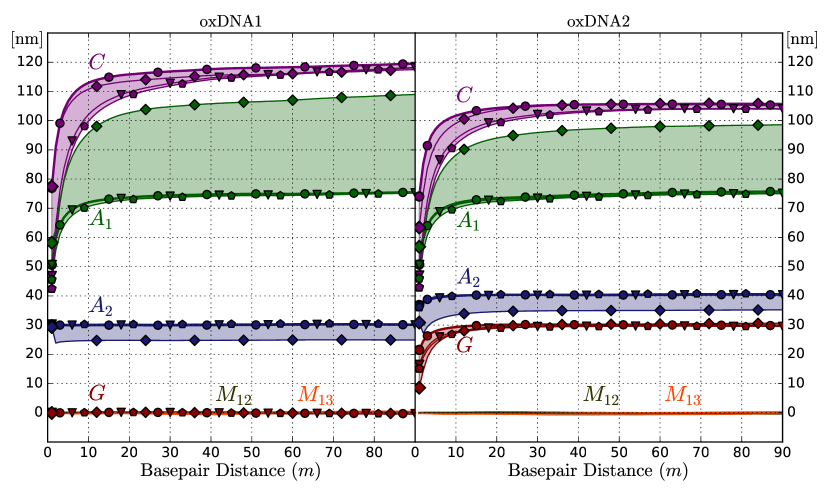
Figure 8: Elements of the $m$-step stiffness matrix as a function of the base-pair distance $m$, extracted from 4 different triad definitions. Data based on Triad I, II, III and IV are shown with triangles, circles, diamonds and pentagons, respectively. Note that the spread in the plateau values of $G$ and $C$ is remarkably small, despite the large differences at $m=1$. For the bending stiffness parameters $A_{1}$ and $A_{2}$, Triads I, II and IV practically yield the same plateau values, while Triad III tends to give quite different values. This is probably due to the fundamentally different definition of the tangent vector in Triad III.

Table 3: Values of the stiffness coefficients (expressed in nm) for oxDNA1 and oxDNA2 for different Triad definitions. The values given here correspond to the plateau values of Fig. 8.

	oxDNA1				oxDNA2
	$A_{1}$	$A_{2}$	C	G	$A_{1}$	$A_{2}$	C	G
Triad I	76	30	120	0.1	76	40	105	29.8
Triad II	75	30	118	0.2	75	40	104	29.6
Triad III	109	25	118	-0.3	99	35	106	30.7
Triad IV	75	30	118	0.1	75	41	104	29.6

Sequence Dependence

So far we have ignored any sequence-dependent effects in oxDNA by considering average base-pair interaction coefficients. This is expected to be a valid approximation for typical and sufficiently long DNA sequences (i.e. consisting of hundreds of base pairs), for which such effects are averaged out.

In order to explore the impact of sequence-dependent interactions, we have repeated the analysis of the main text for some special choices of sequences. The results, for both oxDNA1 and oxDNA2, are summarized in Fig. 9 and Table 4. All parameters exhibit relatively small variations (within 15 %), and $G$ remains significantly non-zero in all cases for oxDNA2.

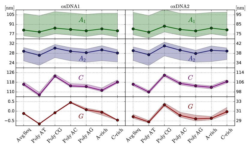
Figure 9: Plateau values of the elastic constants, calculated in the same way as described in the main text, for some specific sequences of dsDNA. The indicated values are the mean values over the 4 different triad definitions, while the shaded region indicates the range of observed values. From these plots it is clear that the interaction parameters are only weakly sequence-dependent. Furthermore, we see again that only for oxDNA2 the coupling term $G$ is significantly non-zero. A-rich and C-rich indicate sequences which contained approximately 83% of A and C respectively. The ‘Poly’-sequences consisted out of repetitions of two bases. Numerical values can be found in Table 4. For comparison we included the values found with the averaged sequence parameters.

Table 4: The elastic constants for some specific sequences of dsDNA. These are the numerical values of the quantities plotted in Fig. 9, averaged over all four triad definitions. More information can be found in the caption of Fig. 9

	oxDNA1				oxDNA2
	$A_{1}$	$A_{2}$	C	G	$A_{1}$	$A_{2}$	C	G
AvgSeq	82.7	28.9	116.3	-0.12	80.3	39.1	104.4	29.9
Poly AT	80.0	27.2	107.6	-0.65	76.9	37.4	097.9	28.8
Poly CG	85.6	30.2	123.0	-0.08	83.1	41.1	111.9	32.3
Poly AC	83.6	28.9	115.0	-0.45	79.8	39.3	105.1	30.2
Poly AG	81.6	28.3	114.5	-0.08	78.2	37.9	103.0	29.4
A-rich	84.5	29.4	111.3	-0.05	81.1	39.3	101.9	29.5
C-rich	81.6	28.1	118.1	-0.46	79.3	38.9	106.6	30.9

oxRNA

Finally one could wonder about the magnitude of twist-bend coupling for dsRNA, a double-helical molecule with major and minor grooves. However, this double helix is in A-form, which differs from the B-form dsDNA studied in the main text. One of the differences is that the A-form has larger grooves, but there are more structural differences between the two. This makes the effect of the larger grooves on the magnitude of the twist-bend coupling hard to predict. Here we only confirmed that symmetry breaking results in a non-zero coupling, but it is not a priori clear which factors or structural parameters influence its magnitude.

To address this question more carefully, we again resort to computer simulations. This could be done quite easily, since the authors of oxDNA also provide a simulation code for RNA, called oxRNA. In Fig. 10 the interaction parameters from these simulations are presented. It is important to note here that both oxRNA1 and oxRNA2 have major and minor grooves, and the difference between the two is in modelling of electrostatic effects. For both models it is clear that $G$ is manifestly non-zero, while the other two off-diagonal terms, $M_{12}$ and $M_{13}$, lie very close to zero. This is a signature of the existence of major and minor grooves. The value of $G$ lies around $10$ nm, which is smaller than the one found for oxDNA. In Fig. 11 the bending and twisting persistence length of RNA ($l_{\text{b}}$ and $l_{\text{t}}$, respectively) are shown. Although the magnitude of $l_{\text{b}}$ and $l_{\text{t}}/2$ (34 nm and 73 nm for oxRNA2, respectively) are lower than the experimentally determined ones (J. Lipfert et al. PNAS 111, 15408 (2014)), they are in line with previous estimates in oxRNA (C. Matek et al. J. Chem. Phys. 143, 243122 (2015)).

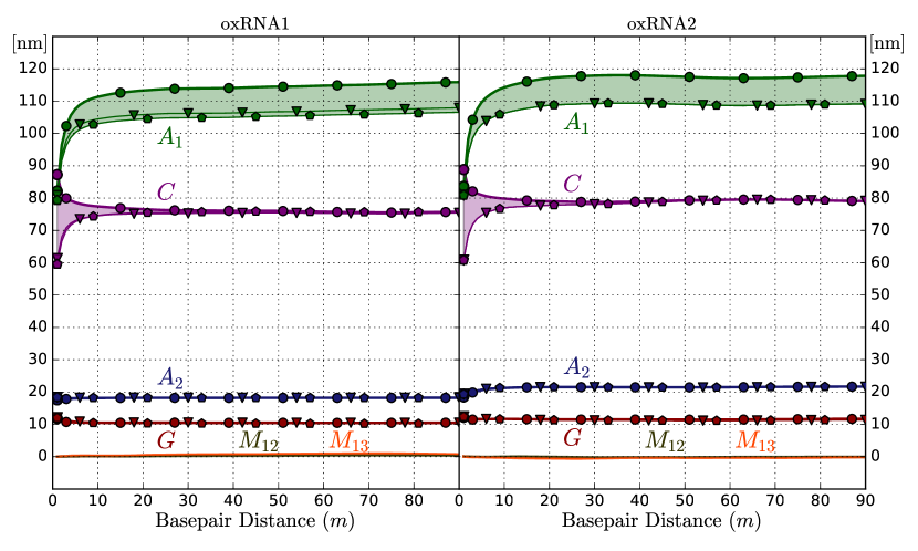
Figure 10: The elastic constants obtained from oxRNA, similar to Fig. 8. The simulation and extraction scheme was the same as in the main text. dsRNA has major and minor grooves, and again we observe that $G$ is non-zero, while the other two mixed interaction parameters ($M_{12}$ and $M_{23}$) are very close to zero. It is important to note that both oxRNA1 and oxRNA2 have major and minor grooves, but have different implementations of the electrostatic interactions. Note that, to enhance the readability of the plot, we have omitted the data from Triad III, as they yielded significantly different plateau values ($A_{1}=103$ nm, $A_{2}=45$ nm, $C=50$ nm and $G=31$ nm, but still $M_{12},M_{13}\approx 0$, for oxRNA2). This is likely due to the tilted base-pair planes with respect to the helical axis of the A-form helix, which affects this particular choice of the tangents.

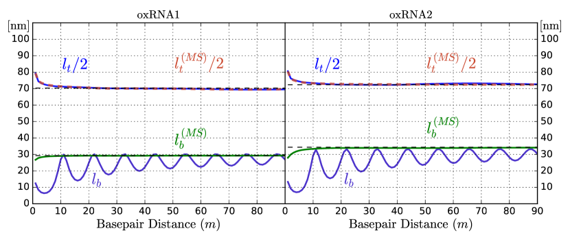
Figure 11: The bending and twisting persistence length of dsRNA, similar to Fig. 5 of the main text, as obtained from oxRNA. The values agree well with the ones reported for oxRNA.

References

- Bryant, Oberstrass, and Basu 2012 Z. Bryant, F. C. Oberstrass, and A. Basu, “Recent developments in single-molecule DNA mechanics,” Curr. Opin. Struct. Biol. 22, 304–312 (2012).
- Marko and Siggia 1995 J. F. Marko and E. D. Siggia, “Stretching DNA,” Macromolecules 28, 8759–8770 (1995).
- Moroz and Nelson 1998 J. D. Moroz and P. Nelson, “Entropic elasticity of twist-storing polymers,” Macromolecules 31, 6333–6347 (1998).
- Ubbink and Odijk 1999 J. Ubbink and T. Odijk, “Electrostatic-undulatory theory of plectonemically supercoiled DNA,” Biophys. J. 76, 2502–2519 (1999).
- Nelson, Radosavljevic, and Bromberg 2002 P. Nelson, M. Radosavljevic, and S. Bromberg, Biological physics: energy, information, life (W.H. Freeman and Co., New York, 2002).
- Bustamante, Bryant, and Smith 2003 C. Bustamante, Z. Bryant, and S. B. Smith, “Ten years of tension: single-molecule DNA mechanics,” Nature 421, 423–427 (2003).
- Marko and Siggia 1994a J. F. Marko and E. D. Siggia, “Fluctuations and supercoiling of DNA,” Science 265, 506–508 (1994a).
- Strick et al. 1996 T. Strick, J.-F. Allemand, D. Bensimon, A. Bensimon, and V. Croquette, “The elasticity of a single supercoiled DNA molecule,” Science 271, 1835–1837 (1996).
- Lipfert et al. 2010 J. Lipfert, J. W. Kerssemakers, T. Jager, and N. H. Dekker, “Magnetic torque tweezers: measuring torsional stiffness in DNA and PRecA-DNA filaments,” Nat. Methods 7, 977–980 (2010).
- Lipfert et al. 2011 J. Lipfert, M. Wiggin, J. W. Kerssemakers, F. Pedaci, and N. H. Dekker, “Freely orbiting magnetic tweezers to directly monitor changes in the twist of nucleic acids,” Nat. Commun. 2, 439 (2011).
- Nomidis et al. 2017 S. K. Nomidis, F. Kriegel, W. Vanderlinden, J. Lipfert, and E. Carlon, “Twist-bend coupling and the torsional response of double-stranded DNA,” Phys. Rev. Lett. 118, 217801 (2017).
- Marko and Siggia 1994b J. Marko and E. Siggia, “Bending and twisting elasticity of DNA,” Macromolecules 27, 981–988 (1994b).
- Lankaš et al. 2000 F. Lankaš, J. Šponer, P. Hobza, and J. Langowski, “Sequence-dependent elastic properties of DNA,” J. Mol. Biol. 299, 695–709 (2000).
- Mohammad-Rafiee and Golestanian 2005 F. Mohammad-Rafiee and R. Golestanian, “Elastic correlations in nucleosomal DNA structure,” Phys. Rev. Lett. 94, 238102 (2005).
- Ouldridge, Louis, and Doye 2010 T. E. Ouldridge, A. A. Louis, and J. P. Doye, “DNA nanotweezers studied with a coarse-grained model of DNA,” Phys. Rev. Lett. 104, 178101 (2010).
- Snodin et al. 2015 B. E. Snodin, F. Randisi, M. Mosayebi, P. Šulc, J. S. Schreck, F. Romano, T. E. Ouldridge, R. Tsukanov, E. Nir, and A. A. Louis, “Introducing improved structural properties and salt dependence into a coarse-grained model of DNA,” J. Chem. Phys. 142, 234901 (2015).
- Salari et al. 2015 H. Salari, B. Eslami-Mossallam, S. Naderi, and M. Ejtehadi, “Extreme bendability of DNA double helix due to bending asymmetry,” J. Chem. Phys. 143, 104904 (2015).
- Šulc et al. 2012 P. Šulc, F. Romano, T. E. Ouldridge, L. Rovigatti, J. P. K. Doye, and A. A. Louis, “Sequence-dependent thermodynamics of a coarse-grained DNA model,” \bibfield journal \bibinfo journal J. Chem. Phys.\ \textbf \bibinfo volume 137,\ \bibinfo eid 135101 (\bibinfo year 2012).
- Sutthibutpong et al. 2016 T. Sutthibutpong, C. Matek, C. Benham, G. G. Slade, A. Noy, C. Laughton, J. P. Doye, A. A. Louis, and S. A. Harris, “Long-range correlations in the mechanics of small DNA circles under topological stress revealed by multi-scale simulation,” Nucl. Acids Res. 44, 9121–9130 (2016).
- Fathizadeh, Eslami-Mossallam, and Ejtehadi 2012 A. Fathizadeh, B. Eslami-Mossallam, and M. R. Ejtehadi, “Definition of the persistence length in the coarse-grained models of DNA elasticity,” \bibfield journal \bibinfo journal Phys. Rev. E\ \textbf \bibinfo volume 86,\ \bibinfo pages 051907 (\bibinfo year 2012).
- Huang 1987 K. Huang, Statistical Mechanics (J. Wiley, 1987).
- Ouldridge, Louis, and Doye 2011 T. E. Ouldridge, A. A. Louis, and J. P. Doye, “Structural, mechanical, and thermodynamic properties of a coarse-grained DNA model,” J. Chem. Phys. 134, 085101 (2011).
- Matek et al. 2015 C. Matek, T. E. Ouldridge, J. P. Doye, and A. A. Louis, “Plectoneme tip bubbles: Coupled denaturation and writhing in supercoiled DNA,” Scientific Reports 5, 7655 (2015).
- Lankaš et al. 2003 F. Lankaš, J. Šponer, J. Langowski, and T. E. Cheatham, “DNA basepair step deformability inferred from molecular dynamics simulations,” Biophys. J. 85, 2872–2883 (2003).
- Eslami-Mossallam and Ejtehadi 2009 B. Eslami-Mossallam and M. Ejtehadi, “Asymmetric elastic rod model for DNA,” Phys. Rev. E 80, 011919 (2009).
- Brackley, Morozov, and Marenduzzo 2014 C. Brackley, A. Morozov, and D. Marenduzzo, “Models for twistable elastic polymers in brownian dynamics, and their implementation for LAMMPS,” J. Chem. Phys. 140, 135103 (2014).
- Marko 1997 J. Marko, “Stretching must twist DNA,” EPL 38, 183 (1997).
- Gore et al. 2006 J. Gore, Z. Bryant, M. Nöllmann, M. U. Le, N. R. Cozzarelli, and C. Bustamante, “DNA overwinds when stretched,” Nature 442, 836–839 (2006).
- Lionnet and Lankaš 2007 T. Lionnet and F. Lankaš, “Sequence-dependent twist-stretch coupling in DNA,” Biophys. J. 92, L30–L32 (2007).
- Upmanyu et al. 2008 M. Upmanyu, H. Wang, H. Liang, and R. Mahajan, “Strain-dependent twist–stretch elasticity in chiral filaments,” J. R. Soc. Interface 5, 303–310 (2008).
- Sheinin and Wang 2009 M. Y. Sheinin and M. D. Wang, “Twist–stretch coupling and phase transition during DNA supercoiling,” Phys. Chem. Chem. Phys. 11, 4800–4803 (2009).
- Lipfert et al. 2014 J. Lipfert, G. M. Skinner, J. M. Keegstra, et al., “Double-stranded RNA under force and torque: Similarities to and striking differences from double-stranded DNA,” PNAS 111, 15408–15413 (2014).
- Dršata et al. 2014 T. Dršata, N. Špačková, P. Jurečka, M. Zgarbová, J. Šponer, and F. Lankaš, “Mechanical properties of symmetric and asymmetric DNA A-tracts: implications for looping and nucleosome positioning,” Nucl. Acids Res. 42, 7383–7394 (2014).
- Lepage, Képès, and Junier 2015 T. Lepage, F. Képès, and I. Junier, “Thermodynamics of Long Supercoiled Molecules: Insights from Highly Efficient Monte Carlo Simulations,” \bibfield journal \bibinfo journal Biophys. J.\ \textbf \bibinfo volume 109,\ \bibinfo pages 135–143 (\bibinfo year 2015).
- Fathizadeh, Schiessel, and Ejtehadi 2015 A. Fathizadeh, H. Schiessel, and M. Ejtehadi, “Molecular dynamics simulation of supercoiled DNA rings,” Macromolecules 48, 164–172 (2015).
- Becker and Everaers 2009 N. B. Becker and R. Everaers, “DNA nanomechanics: How proteins deform the double helix,” J. Chem. Phys. 130, 04B602 (2009).
- Marko 2015 J. F. Marko, “Biophysics of protein-DNA interactions and chromosome organization,” Physica A 418, 126–153 (2015).