Evaluation of DVFS techniques on modern HPC processors and accelerators for energy-aware applications

Abstract

Energy efficiency is becoming increasingly important for computing systems, in particular for large scale HPC facilities. In this work we evaluate, from an user perspective, the use of Dynamic Voltage and Frequency Scaling (DVFS) techniques, assisted by the power and energy monitoring capabilities of modern processors in order to tune applications for energy efficiency. We run selected kernels and a full HPC application on two high-end processors widely used in the HPC context, namely an NVIDIA K80 GPU and an Intel Haswell CPU. We evaluate the available trade-offs between energy-to-solution and time-to-solution, attempting a function-by-function frequency tuning. We finally estimate the benefits obtainable running the full code on a HPC multi-GPU node, with respect to default clock frequency governors. We instrument our code to accurately monitor power consumption and execution time without the need of any additional hardware, and we enable it to change CPUs and GPUs clock frequencies while running. We analyze our results on the different architectures using a simple energy-performance model, and derive a number of energy saving strategies which can be easily adopted on recent high-end HPC systems for generic applications.

1 Introduction

The performances of current HPC systems are increasingly bounded by their energy consumption, and one expects this trend to continue in the foreseeable future. On top of technical issues related to power supply and thermal dissipation, ownership costs for large computing facilities are increasingly dominated by the electricity bill. Indeed computing centers are considering the option to charge not only running time, but also energy dissipation, in order to encourage users to optimize their applications for energy efficiency.

For HPC users there are different approaches to reduce the energy cost of a given application. One may adjust available power-related parameters of the systems on which applications run [1, 2], or one may decide to tune codes in order to improve their energy efficiency [3]. Following the former approach, recent processors support Dynamic Voltage and Frequency Scaling (DVFS) techniques, making it possible to tune the processor clock frequency. The software approach, on the other side, may be a winner in the long run, but it involves large programming efforts and also depends on reliable and user-friendly tools to monitor the energy costs of each kernel of a possibly large code.

This papers offers a contribution in the first direction, but also, while not discussing in details the software approach to energy optimizations, considers several reliable and user-friendly software tools and performance models which may eventually support the second direction too.

We focus on simple techniques to monitor the energy costs of key functions of large HPC programs, assessing the energy saving and the corresponding performance cost that one can expect – for a given application code – by a careful tuning of processor (i.e. CPU and GPU) clocks on a function-by-function basis. In other words, we explore the energy-optimization space open in a situation in which – due to code complexity, or for other reasons – one would like to leave the running code unchanged, or – at most – annotate it.

1.1 Related Works

Processors power accounts for most of the power drained by computing systems [4] and DVFS techniques were introduced to tailor a processor clock and its supply voltage. This approach has an immediate impact on the processor drained power, since – to first approximation – the power dissipation of gates is given by:

$$P_{avg}=fCV^{2}+P_{static}$$

where $P_{avg}$ is the average total power, $f$ the working frequency, $C$ the capacitance of the transistor gates, $V$ the supply voltage, while $P_{static}$ is the static power, drained also while idle, accounting for example for leakage currents.

Power reduction does not automatically translate to energy saving, since the average power drain of the system has to be integrated over the application execution time (or time-to-solution, $T_{S}$) to obtain the energy consumed by the application (or energy-to-solution, $E_{S}$):

$$E_{s}=T_{s}\times P_{avg}$$

so an increase in $T_{S}$ may actually increase $E_{S}$, in spite of a lower average power drain $P_{avg}$. This is a well known phenomenon motivating the convenience in some cases to run at maximum clock frequency, no matter the power needed, in order to reach the solution as soon as possible and then enter a low power idle state: this is the so called “Race-to-idle”.

Nowadays DVFS is routinely used to ensure that processors stay within an allowed power budget, in order to run applications without over-heating the processor, and allowing short frequency bursts when possible. The potential of DVFS to reduce energy-to-solution for a complete application has been questioned with several arguments [5], e.g. since DVFS acts mainly on dynamic power, the trend of increasing ratio between static vs dynamic power drain reduces its effectiveness in lowering energy-to-solution. However, DVFS techniques have recently gained fresh attention in various research works especially in the context of large parallel HPC contexts [6], where saving even a small fraction of a very large energy budget may have a significant impact.

Research work has focused in particular on communication phases, when processes within large parallel MPI applications stop their execution, waiting for data exchanges. These phases are indeed the best candidates to lower the CPU clock with minimal impact on overall performance [7, 8]. However, from the point of view of performances, it is good practice to overlap communication and computation whenever possible [9]. Consequently, in several applications, in particular lattice based computations (such as the one we adopt as a benchmark in this paper), communication phases are often fully overlapped with computation, making this strategy less effective.

Other research works focused on the possibility to reduce the clock frequency in the case of an imbalance between the computational load of multi-task applications, allowing to reduce the clock frequency only for idle ranks [10]. But again, for the broad range of massively parallel computations, one tries to balance the computational load evenly on each of the computing threads or processes, reducing the impact of this opportunity.

Finally, the widespread adoption of accelerators in HPC systems means that the largest fraction of the power drained by computing systems is no more ascribable to CPUs. For instance, with the advent of multi-GPU compute nodes, where up to 8 dual GPU boards are hosted on a single computing node, up to $\simeq 75\%$ of the power could be drained by GPUs, with CPUs accounting for only $5-10\%$ of the total energy budget . Consequently, as recent GPUs improve their support of DVFS, in many cases allowing for a fine grained frequency selection [2, 11, 12], various studies focused on the optimization space made available by tuning GPU clock frequencies.

1.2 Contributions

In a previous work [13] we analyzed the tradeoff between computing performance and energy efficiency for a typical HPC workload on selected low-power systems. We considered low-power Systems on a Chip (SoCs) since they are intended for mobile applications, so they provide several advanced power monitoring and power saving features, but also in view of a prospective usage as building blocks for future HPC systems [14]. Given the increasing interest in controlling and reducing energy dissipation, recent high-end processors have started to support advanced power-saving and power-monitoring technologies, similar to those early adopted in low-power processors  [15, 16].

In this paper we perform a similar analysis on state-of-the-art HPC compute engines (hi-end processors and accelerators) addressing energy-performance tradeoffs for typical HPC workloads. For this purpose, we compare different architectures from the energy efficiency point of view, adopting some workload benchmarks that we had used earlier to compare CPUs and various accelerators from the sole point of view of performances [17, 18]. We use the same application benchmark as in [13], a Lattice Boltzmann code, widely used in CFD and optimized for several architectures [19, 20, 21], this workload is well suited for benchmarking purposes because its two most critical functions are respectively strongly memory- and compute-bound. Lattice Boltzmann implementations were recently used in other works, e.g. in [22] presenting a similar analysis for the Intel Sandy Bridge processor.

At variance with previous works such as [8, 10], we do not attempt to provide an automatic tuning of processors frequencies nor an automatic tool able to identify where to apply frequency scaling. As it is the case for various widely known “computational challenges” applications, we assume the users to already know the code functions where most of the computing time is spent and moreover to already know which are the compute- or memory-bound parts. This knowledge is assumed to derive e.g. from a previous performance optimization, which could be complemented with an additional optimization towards energy efficiency. We aim therefore with this work to offer an in-depth overview of possible energy optimization steps available on recent common HPC architectures, exploitable by HPC users that are already familiar with performance optimizations of their codes.

In this paper we follow an approach close to the one presented in [1] for an Intel CPU, exploring the optimization space for all possible CPU frequencies, but considering a more recent Intel Haswell architecture and without utilizing custom power measurement hardware. We also take into account GPU architectures, as recently done also in [2], but using the more recent K80 architecture and a larger set of frequencies.

Our hardware testbed is a high-end HPC node of the COKA (COmputing on Kepler Architecture) Cluster, hosted at the University of Ferrara. Each node in this cluster has 2 $\times$ Intel Haswell CPUs and 8 $\times$ dual GPU NVIDIA K80 boards. We use two implementations of the same algorithm, previously optimized respectively for CPUs and GPUs [20, 23], with different configurations and compilation options.

We make an extensive set of power and performance measurements of the critical kernels of the code, varying clock parameters for the hardware systems that we test. Using this information we assess the available optimization space in terms of energy and performance, and the best trade-off points between these conflicting requirements. We do so for individual critical routines, as we try to understand the observed behavior using some simple but useful combined models of performance, power and energy.

We then investigate the possibility of tuning the clock frequency on a function by function basis, while running a full simulation, in order to run each function as energy-efficiently as possible. We discuss our findings with respect to a simple energy-performance model. Finally, we demonstrate the actual energy saving potential, measuring the different energy consumptions of a whole computing node, while performing a full simulation at different GPU clock frequencies.

2 The application benchmark

Lattice Boltzmann methods (LB) are widely used in computational fluid dynamics, to describe flows in two and three dimensions. LB methods – discrete in position and momentum spaces – are based on the synthetic dynamics of populations sitting at the sites of a discrete lattice. At each time step, populations hop from lattice-site to lattice-site and then incoming populations collide among one another, that is, they mix and their values change accordingly. LB models in $n$ dimensions with $p$ populations are labeled as $DnQp$; we consider a $D2Q37$ model describing the thermo-hydrodynamical evolution of a fluid in two dimensions, and enforcing the equation of state of a perfect gas ($p=\rho T$) [24, 25]; this model has been used for large scale simulations of convective turbulence (see e.g., [26, 27]). A set of populations ($f_{l}({\bm{x}},t)~{}l=1\cdots 37$), defined at the points of a discrete and regular lattice and each having a given lattice velocity $\bm{c}_{l}$, evolve in (discrete) time according to the following equation:

$$f_{l}({\bm{x}},t+{\Delta t})=f_{l}({\bm{x}}-{\bm{c}}_{l}{\Delta t},t)-\frac{{\Delta t}}{\tau}\left(f_{l}({\bm{x}}-{\bm{c}}_{l}{\Delta t},t)-f_{l}^{(eq)}\right)$$ (1)

The macroscopic variables, density $\rho$, velocity $\bm{u}$ and temperature $T$ are defined in terms of the $f_{l}(x,t)$ and of the $\bm{c}_{l}$s; the equilibrium distributions (${f}_{l}^{(eq)}$) are themselves a function of these macroscopic quantities [28]. In words, populations drift from different lattice sites (propagation), according to the value of their velocities and, on arrival at point ${\bm{x}}$, they change their values according to Eq. 1 (collision). One can show that, in suitable limiting cases, the evolution of the macroscopic variables obeys the thermo-hydrodynamical equations of motion of the fluid. Inspection of Eq. 1 shows that the algorithm offers a huge degree of easily identifiable parallelism; this makes LB algorithms popular HPC massively-parallel applications.

An LB simulation starts with an initial assignment of the populations, in accordance with a given initial condition at $t=0$ on some spatial domain, and iterates Eq. 1 for each point in the domain and for as many time-steps as needed. At each iteration two critical kernel functions are executed: i) propagate moves populations across lattice sites collecting at each site all populations that will interact at the next phase (collide). Consequently, propagate moves blocks of memory locations allocated at sparse addresses, corresponding to populations of neighbor cells; ii) collide performs all mathematical steps associated to Eq. 1 in order to compute the population values at each lattice site at the next time step. Input data for collide are the populations just gathered by propagate. collide is the floating point intensive step of the code.

It is very helpful for our purposes that propagate, involving a large number of sparse memory accesses, is strongly memory-bound; collide, on the other hand, is strongly compute-bound, and the performance of the floating-point unit of the processor is here the ultimate bottleneck.

3 Experimental setup

All our tests were run on a single node of the COKA Cluster at the University of Ferrara. Each node has 2 $\times$ Intel Haswell E5-2630v3 CPUs and 8 $\times$ dual GPU NVIDIA K80 Boards.

We use processor-specific implementations of the LB algorithm of Sec. 2, exploiting a large fraction of the available parallelism of the targeted architectures. On the GPU we run an optimized CUDA code, developed for large scale CFD simulations [17, 18], while on the CPU we run an optimized C version [29, 30] using AVX2 intrinsics exploiting the vector units of the processor and OpenMP for multi-threading within the cores.

For all codes and for each critical kernel we perform runs at varying values of the clock frequencies, and log power measurements on a fine-grained time scale. For both of our target processors we read specific hardware registers/counters able to provide energy or power readings. This simple approach has been validated with hardware power meters by third parties studies for recent NVIDIA GPUs and Intel CPUs [15], showing that it produces accurate results [16, 31]. In this approach we cannot monitor the power drain of the motherboard and other ancillary hardware; recent studies have shown however that the power drain of those components is approximately constant in time and weakly correlated with code execution [15, 32]. In-band measurements may also introduce overheads, which in turn may affect our results. In this regard, we checked that performance degradation due to power measurements is negligible and measured the power dissipation of the sole measurement code, verifying that it is less than +5% of the baseline power dissipation.

We developed a custom library to manage power/energy data acquisition from hardware registers; it allows benchmarking codes to directly start and stop measurements, using architecture specific interfaces, such as the Running Average Power Limit (RAPL) for the Intel CPU and the NVIDIA Management Library (NVML) for the NVIDIA GPU. Our library also lets benchmarking codes to place markers in the data stream in order to have an accurate time correlation between the running kernels and the acquired power/energy values. For added portability of the instrumentation code, we exploited the PAPI Library [31] as a common API for energy/power readings for the different processors, partially hiding architectural details. The wrapper code, exploiting the PAPI library, is available for download as Free Software [33].

Our benchmark codes are also able to change the processor clock frequencies from within the application. The code version for Intel CPUs uses the acpi_cpufreq driver of the Linux kernel , able to set a specific frequency on each CPU core by calling the cpufreq_set_frequency() function. The Userspace cpufreq governor has to be loaded in advance, in order to disable dynamic frequency scaling and to be able to manually select a fixed CPU frequency. As shown later, we also tested other clock governors in our benchmarks, such as the Performance, Powersave and Ondemand ones. The NVIDIA GPUs code changes the GPU processor and memory frequency, using the NVML library and in particular the nvmlDeviceSetApplicationsClocks() function.

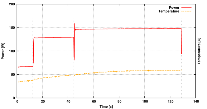
(a) Power drain while executing 1000 iterations of the propagate function, followed by 1000 iterations of the collide function on one of the two GPUs of an NVIDIA K80 accelerator at a requested GPU clock frequency of 875MHz. As power exceeds the designed TDP (150W), frequency is automatically reduced to limit the power drain. The plot also shows the processor temperature.

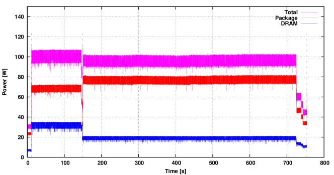
(b) Power drain on one of the two CPUs at a fixed CPU clock frequency of 2.4GHz for the same tests as in the previous panel; in this case we show separately the power drained by the processor and by the memory system and their sum.

Figure 1: Plot of the power drain during the run of the two critical kernels (propagate and collide) of our benchmark code; GPU data at top, CPU data at bottom.

The computationally critical section of a production run of our code performs subsequent iterations of: the propagate function, the application of boundary conditions and then the collide function as described in Sec. 2. Boundary conditions depending on the details of the specific simulation, have a marginal computational cost in typical simulations (of the order of $1-2\%$), so we neglect this computational phase in our detailed analysis (but the corresponding routines are included in the full code).

We have instrumented the two critical functions and performed several test runs, monitoring the power/energy consumption. All tests adopt double precision for floating point data, the same lattice size ($1024\times 8192$) and the same number of iterations ($1000$).

Fig. 1 shows a sample of our typical raw data; Fig. 1a shows the measured power drain on one of the 2 GPUs of an NVIDIA K80 board at a fixed GPU frequency of 875MHz; additionally, GPU temperature during the run is obtainable (and plotted in the figure). Fig. 1b shows the same data for one Intel CPU at a fixed CPU frequency of 2.4GHz. On the Haswell CPU we have two energy readings [16]: the Package Energy (that we divide by the elapsed time to convert to power and plot in red) and the DRAM Energy (again converted to power and plotted in blue). The sum of the two readings – the total power drained during the run – is plotted in magenta.

The patterns shown in Fig. 1 are qualitatively easy to understand: we see a power surge during the execution of propagate and a further large power figure during the execution of collide; Fig. 1a tells us that on GPUs collide is more power intensive than propagate while Fig. 1b informs us that in the latter routine the power drain of the memory system is comparatively larger, as expected in a memory-bound section of the code. As code execution ends, power drain quickly plummets. An interesting feature in Fig. 1a is the short power spike as collide starts executing: in this case power briefly exceeds the TDP for this processor (150W) and a self-preservation mechanism reduces frequency to bring power down to acceptable levels; this mechanism will have an impact on our analysis, as discussed later.

CPU data has larger fluctuations than GPU data, since samples for the former are collected at 100Hz, while for the latter we have averages of longer time series, collected at 10Hz, since for higher sample frequency, the NVML component of the PAPI library starts to return repeated samples. However, in both cases, time accuracy is enough to capture all interesting details.

We recorded data for all values of the clock frequency of the processor at a fixed memory frequency of 2133 MHz (CPU) and 2505 MHz (GPU): indeed – at variance with low-power processors [13] – the systems that we test run at a fixed frequency of the memory interface. This data is the starting point for the analysis shown in the following .

4 Performance and Energy models

In this section, we consider figures-of-merit useful to assess the energy cost of a computation and to develop some models that will guide us in the analysis of our experimental data.

We consider the time-to-solution ($T_{S}$) and energy-to-solution ($E_{S}$, in Joule, defined as the average power $P_{avg}$ multiplied by $T_{S}$) metrics and their correlations as relevant and interesting parameters when looking for tradeoffs between conflicting energy and performance targets. Other quantities – e.g. the energy-delay product (EDP) – have been proposed in the literature, in an attempt to define a single figure-of-merit; however we think that correlations between several parameters better highlight the underlying mechanisms; other authors share this attitude (see for instance [22]).

We adopt a simple model that links $E_{S}$ and $T_{S}$, combining the Roofline Model [34], with a simple power model for a generic processor. The Roofline Model identifies in any processor based on the Von Neumann architecture two different subsystems, working together to perform a given computation: a compute subsystem with a given computational performance $C$ in operations-per-second or FLOPS/s (if the workload is mostly floating-point) and a memory subsystem, providing a bandwidth $B$ in words- or bytes-per-seconds, between processor and memory. The ratio $M_{b}=C/B$, specific of each hardware architecture, is the machine-balance [35]. Looking now at a generic target application, the Roofline Model considers that every computational task performs a certain number of operations $O$, operating on $D$ data items to be fetched/written from/onto memory. For any software function, the corresponding ratio $I=O/D$ is the arithmetic intensity, computational intensity or operational intensity [34].

The Roofline Model derives performance estimations combining arithmetic intensity and machine-balance. Using a notation slightly different from the one of the original paper [34], one obtains that to first approximation – e.g., neglecting scheduling details –

$$T_{S}\approx max[T_{c},T_{m}]=max[\frac{O}{C},\frac{D}{B}]=\frac{O}{C}max[1,\frac{DC}{OB}]=\frac{O}{C}max[1,\frac{M_{b}}{I}].$$ (2)

Eq. 2 tells us that $T_{S}$ is a decreasing functions of $C$, as naively expected, but only as long as $M_{b}/I\leq 1$; if this condition is not fulfilled, $T_{S}$ stays constant (and we say that the task is memory-bound). To very good approximation, $C$ is proportional to the processor frequency $f$, so, varying $f$ also modulates $M_{b}$ and one derives that

$$T_{S}(f)\propto\frac{1}{f}max[1,\alpha f]$$ (3)

with an appropriate constant $\alpha$.

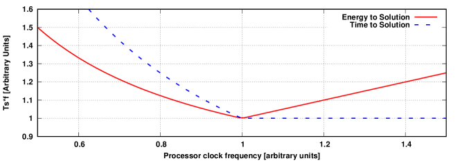
Figure 2: Sketchy behavior of $E_{S}$ and $T_{S}$ as predicted by Eqs. 5 and 3. All quantities in arbitrary units; the frequency value at which $I=M_{b}$ is normalized to 1.

To relate power dissipation $P$ and $f$ we assume a simple linear behavior, ignoring more complex effects such as the leakage current increase with temperature and the voltage change often associated with frequency scaling:

$$P(f)\approx m~{}f+P_{s}$$ (4)

where $P_{s}$ accounts for leakage currents and for the static power drained by parts of the system not used in the specific task.

Combining Eq. 3 and Eq. 4, we have:

$$E_{S}=P(f)\times T_{S}(f)\propto(m+\frac{P_{s}}{f})~{}max[1,\alpha~{}f]$$ (5)

This equation shows that, as we increase $f$, $T_{S}$ and $E_{S}$ both decrease provided that $\alpha f\leq 1$; however, as soon as $\alpha f>1$, increasing $f$ becomes useless, as $E_{S}$ starts to increase again while $T_{S}$ remains constant.

This behavior, sketchly shown in Fig. 2, tells us that the matching of $M_{b}$ and $I$, that in the Roofline Model is relevant for performance, is an equally critical parameter for energy efficiency, as noticed also in [36] and in [37]: indeed, $M_{b}/I\approx 1$ gives the best performance and at the same time the lowest energy dissipation.

Seen from a different perspective we have a duality between complementary approaches: software optimizations for a specific architecture change $I$ to adapt to a given $M_{b}$ while, changing clock frequencies we try to match $M_{b}$ to a given $I$.

5 Data analysis

We plot our results for $E_{S}$ vs. $T_{S}$ in Figs. 3 and 4, showing experimental values for the propagate and collide kernels, for both processors and for all available clock frequencies.

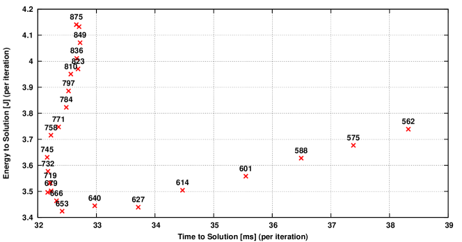
(a) Propagate

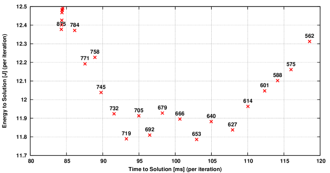
(b) Collide

Figure 3: $E_{S}$ vs $T_{S}$ for the propagate and collide functions, measured on the GPU; labels are the corresponding clock frequencies $f$ in MHz.

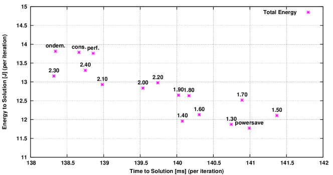
(a) Propagate

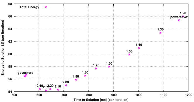
(b) Collide

Figure 4: $E_{S}$ vs $T_{S}$ for the propagate and collide functions, measured on the CPU; labels are the corresponding clock frequencies $f$ in GHz.

At the qualitative level, the results of Figs. 3 and 4 have a slightly diverging behavior across the two architectures; GPU data show a correlated decrease of $E_{S}$ and $T_{S}$ till, at some $E_{S}$, the trend reverses, with $E_{S}$ sharply rising again.

CPU data for propagate on the other hand shows that $T_{S}$ is almost constant ($T_{S}$ changes by $\approx~{}4\%$, while the clock frequency changes by a factor 2), while $E_{S}$ increases by $\simeq 10\%$ as $T_{S}$ decreases. On the same processor, collide shows a gentle correlated decrease of $E_{S}$ and $T_{S}$ for all frequencies that we are able to control. The best $T_{S}$ values shown in the plot are obtained using default cpufreq governors: Performance, Ondemand and Conservative. These default governors allows the processor to use so-called Turbo Boost frequencies, enabling the processor to run above its nominal operating frequency, but this happens at a significant energy cost.

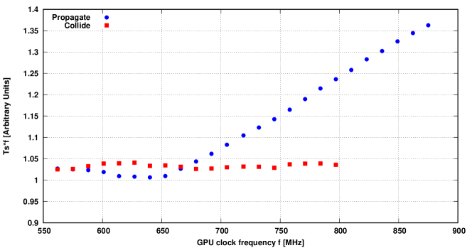
Figure 5: $(f~{}T_{S})$ as a function of $f$ for propagate and collide, running on a GPU. $(f~{}T_{S})$ is constant as long as $M_{b}/I\leq 1$, corresponding to a compute-bound regime; increasing values of $(f~{}T_{S})$ indicate a memory-bound regime.

We now compare our data with the model of the previous section, starting from an analysis of GPU data. A qualitative comparison of data with the model suggests that both routines become memory-bound at some value of the clock frequency; we check this assumption in Fig. 5 where we show (in arbitrarily rescaled units) the product $(f~{}T_{S})$ as a function of $f$ for both kernels: as long as $T_{S}$ scales as $1/f$, $(f~{}T_{S})$ has to take a constant value. We see that for collide this is true up to $f<800$ MHz while for propagate the change happens already at $f\simeq 650$ MHz. Our model would then imply that at those frequencies the two functions become respectively memory-bound.

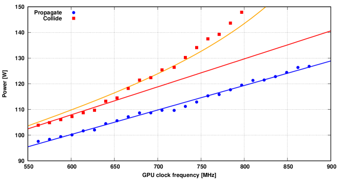
Figure 6: Power measurements on a GPU, running the propagate and collide kernels. the straight lines are the corresponding linear fits (Eqs. 6 and 7), while the curve is a fit of the non-linear power drain for collide at $f\geq 650$ MHz (see text for details).

This analysis justifies the very good agreement of propagate with our model: $E_{S}$ and $T_{S}$ decrease as we increase frequency and then (in our case at $f\geq 650$ MHz) increasing frequency further does not improve $T_{S}$ but increases $E_{S}$. The same behavior is qualitatively similar for collide but not exactly as predicted. To further clarify the situation, we plot in Fig. 6 the power drained by the processor as a function of $f$. For propagate, we observe a linear behavior over the whole frequency range:

$$P(W)=42.94+0.096~{}f.$$ (6)

For collide, the linear behavior is valid only for frequencies $f<650$ Mhz. In this range a fit analogous to the previous one yields

$$P(W)=42.50+0.109~{}f.$$ (7)

As the clock frequency increases beyond $\simeq 650$ MHz, power drain for the collide kernel grows much faster (we model the behavior in this range on purely phenomenological grounds as an additional contribution $P(f)(W)=0.005~{}e^{0.0099f}$); finally, the points on the plot at $f\simeq 800$ MHz and beyond do not describe correctly the actual situation, as the clock governor takes over frequency control, trying to keep the processor within the allowed power budget; as a consequence the actual operating clock frequency is most probably not the one requested by our code. This suggests that collide data points in Fig. 5 beyond $800$ MHz do not reflect a memory-bound regime.

Summing up, we conclude that our model describes accurately the behavior of the propagate kernel while for collide we cannot be conclusive, as we enter a power regime at which we are unable to control the clock frequency before we enter the memory-bound regime. This is related to the fact that collide has a particularly high operational intensity: $I\approx 13.3$, while the two architectures have a theoretical maximum (i.e. computed taking into account maximum Turbo/Auto -boost frequencies) $M_{b}$ of $5.61$ for the CPU and $8.08$ for the GPU.

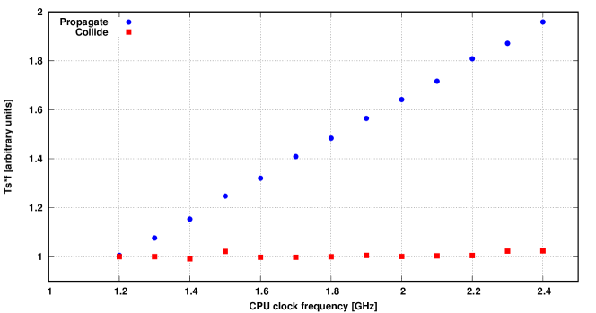
Figure 7: $(f~{}T_{S})$ as a function of $f$ for propagate and collide, running on a CPU, suggesting a memory-bound regime for propagate and a compute-bound regime for collide on the whole $f$ range.

Applying the same line of reasoning to our CPU data, our initial prediction is that propagate is memory-bound on the whole allowed frequency range (since $T_{S}$ is approximately constant) while collide is not, in the frequency range that we control (since we see a constant correlated decrease of $E_{S}$ and $T_{S}$). We check that this is true in Fig. 7, showing again the behavior of $(f~{}T_{S})$ as a function of $f$: we see that this quantity is linearly increasing for propagate and approximately constant for collide. Note that the best option to obtain the highest performance for collide is to let the clock governor free to select the operating frequency; this presumably allow the system to enter Turbo Boost mode, when the power budget permits it, increasing $f$ up to $3.2$ GHz . This comes with some associated $E_{S}$ costs. However, the same strategy for propagate has no advantage in performance while it still has some moderate $E_{S}$ cost. Finally we see that, for both routines, asking the clock governor to apply the powersave strategy, enabling the namesake governor, has an adverse effect on both $T_{S}$ and $E_{S}$.

6 Results and Discussion

Our results allow to draw some preliminary conclusions on possible hardware approaches to energy optimization; from Figs. 3 and 4 one can identify the performance-vs-energy tradeoff made possible by varying the processor frequencies. The first two lines of Table 1 recap this information, listing the best energy saving made possible by these techniques for the two analyzed functions, alongside with the corresponding performance drop that one has to discount. Gains are not large but not negligible either; a simple lesson is that fair energy savings are possible by tuning the processor clock to lower values in all cases in which the code is memory-bound. Many HPC codes today are memory-bound, thus this simple recipe could be usable in a wide range of applications.

An aside result is a direct comparison between the two architectures: for example taking into account the best $E_{S}$ values, the CPU is $\approx 4.5$ times more energy demanding despite being $\approx 6.5$ times slower than the GPU to compute the collide function. This obviously refers only to this code, which is well suited for parallelization on GPU cores.

6.1 Function by function tuning

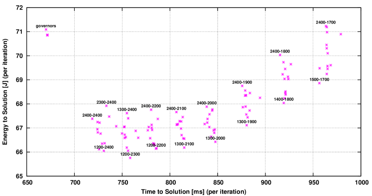
(a) Propagate followed by Collide, CPU.

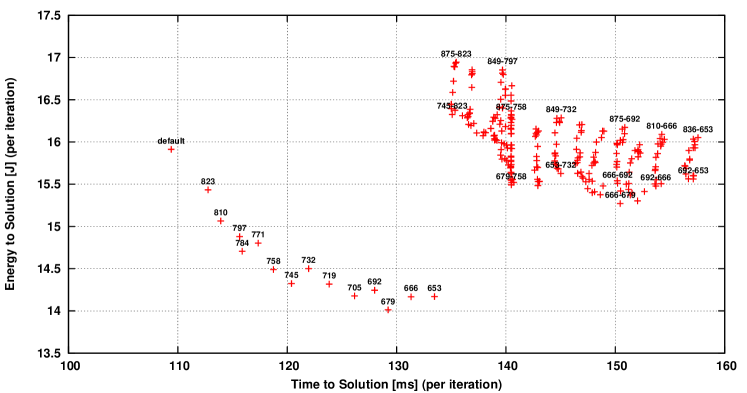
(b) Propagate followed by Collide, GPU.

Figure 8: $E_{S}$ vs $T_{S}$ for the propagate function followed by the collide function, changing the clock frequency on-the-fly. Points are labeled with the used frequencies in MHz: left and right digits represents respectively the frequency set while running the propagate kernel and the collide kernel. A single frequency is reported if the same clock was used for both the functions.

We now consider a further optimization step: one may try to select for each routine the optimal processor frequency, changing it on-the-fly before entering each kernel; this approach may fail if tuning the clock introduces significant additional delays and/or energy costs. Results are shown in Fig. 8, plotting our measured values of $E_{S}$ vs $T_{S}$ for the same combination of the two routines that would apply in a production run, as the processor clocks are set to all possible values before entering each routine; for CPUs this approach is indeed viable, as the overhead associated to on-the-fly clock adjustments is negligible. This is consistent with our independent measurement of the time cost of each clock change ($\approx 10\mu s$) in agreement with similar measurements on Intel Xeon architectures [38]. An interesting feature of the plot is that data points organize in vertical clusters, corresponding to sub-optimal clock frequencies for propagate and clearly showing the adverse effects of a poor frequency match.

For GPUs we see immediately that this technique is not applicable with the available clock adjustment routines, as the time cost of each clock change ($\approx 10ms$) is not negligible w.r.t. the average iteration time. We can anyway select a single clock frequency which is optimal (according to the desired metric) for the whole code.

Table 1 summarizes costs and benefits comparing our best results (in terms of $E_{S}$ minimization) with the corresponding figures related to the default clock governors of the two processors; we see that limited but non-negligible improvements are possible for $E_{S}$ with a fair drop of the code performance.

	GPU		CPU
Routine	$E_{S}$ saving	$T_{S}$ cost	$E_{S}$ saving	$T_{S}$ cost
propagate	$18\%$	$0$	$9\%$	$3\%$
collide	$6\%$	$10\%$	$4\%$	$4\%$
Full code	$11\%$	$10\%$	$7\%$	$8\%$

Table 1: Approximate $E_{S}$ gains made possible by clock tuning and corresponding $T_{S}$ costs.
Percentages referred to $E_{S}$ optimal frequencies.

6.2 Full code on multi-GPUs

The adopted application, given its higher performance on these systems, is commonly run on GPU based HPC clusters. Therefore it may be interesting to measure how much the proposed energy-optimizations could impact on the energy consumption of a whole GPU-based compute node while running a real simulation.

With this aim, we run the original full code without any instrumentation on the 16 GPUs hosted on a single node of the COKA Cluster while measuring its power consumption during the simulation execution. The simulation was run on a $16384\times 8192$ lattice for $10,000$ iterations.

Power measurements, in this case, were performed using the IPMI protocol, in order to acquire data directly from the sensors embedded in the power supplies of the Supermicro SYS-4028GR-TR system. The full node maximum declared power consumption is $3.2$kW. It hosts 8 NVIDIA K80 board accounting for a maximum of $300$W each and thus $2.4$kW in total, giving a $75\%$ of the maximum power drained possibly only by GPUs.

Given that we demonstrated that clock tuning on a function-by-function basis is not convenient for GPUs at this stage, we run the full simulation at different fixed GPU clock frequencies, including one run with the default frequency governor with Autoboost enabled.

Power readings for the full node are reported in Fig. 9a, while the corresponding $E_{S}$ for the application run are reported in Fig. 9b.

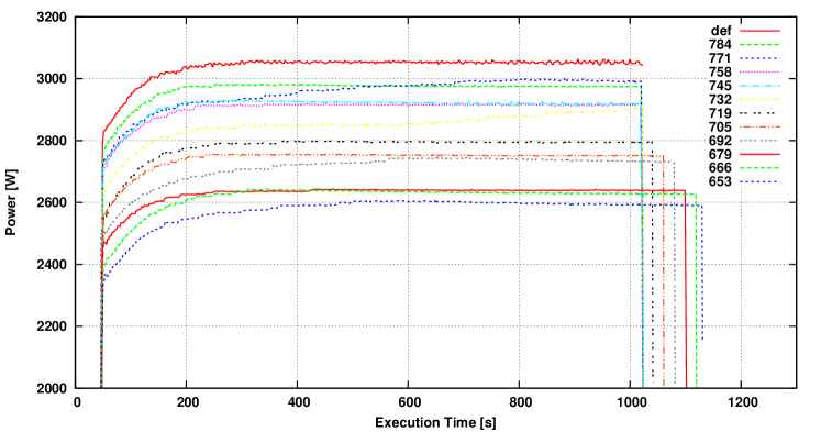
(a) Full node power drain, setting all the GPUs at the same clock frequency, for different clock frequencies. Power drain measured by the power supplies through IPMI.

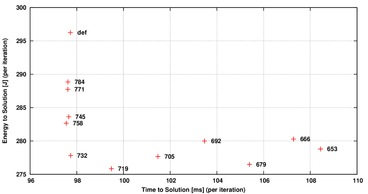
(b) Energy derived from average power drained and execution time, normalized per iteration. GPU clock frequencies as labels in MHz.

Figure 9: Running 10k iterations of a complete Lattice Boltzmann simulation over a $16384\times 8192$ lattice, on a single cluster node, using 16 GPUs, for different GPU frequencies.

As can be seen from Fig. 9b at a specific frequency (i.e. 732MHz) $\approx 7\%$ of the total consumed energy of the computing node can be saved, with respect to the default behavior, without impacting performances.

7 Conclusions

In this paper we have analyzed the potential for energy optimization of an accurate selection of the processor clock, tuning machine balance of the processor to operational intensity of the application. We applied this method to a typical HPC workload on state-of-the-art architectures, discussing the corresponding possible performance costs.

Our approach yields sizeable energy savings for typical HPC workloads with a simple and fast tuning effort; the associated performance costs are easily manageable. The main advantage of this approach is that it can be applied to any production program with a limited amount of easily-applied measurements, not involving additional hardware, or expensive program adjustments.

Some further remarks are in order:

• It is relatively easy to instrument application codes to have accurate energy measurements of key application kernels, using hardware counters and minimally disrupting the behavior and performance of the original code.

• Simple theoretical models – while admittedly unable to capture all details of the $E_{S}$ and $T_{S}$ behavior – still provide a level of understanding that is sufficient to guide optimization strategies.

• An important result is that the best practice for both performance and energy efficiency is to look at the $I$ and $M_{b}$ parameters: if $I\leqslant M_{b}$, reducing $M_{b}$ (e.g. lowering the clock frequency) will reduce $E_{S}$ with a negligible impact on performance; in other words, for compute-bound codes the best strategy is to run the code at the highest sustained processor frequency while, for memory-bound code, decreasing the clock frequency usually reduces $E_{S}$ with essentially no impact on performance. Since many real-life HPC codes today are memory-bound, this practice could be useful for many applications.

• Default frequency governors usually yield the best performances, but do not minimize energy costs; on the other hand, using the lowest frequencies (such as prescribed by the powersave cpufreq governor), is in general a bad choice, from the point of view of both $E_{S}$ and $T_{S}$.

• “on-the-fly” clock adjustment is a viable strategy on recent Xeon processors, while on NVIDIA GPUs the overheads of the clock management libraries makes this strategy hardly useful.

• Highest frequencies, in particular the ones enabled by Auto/Turbo -boost mechanisms, let power drain increase superlinearly with respect to $f$ causing a systematic divergence from our predictions. This may be due to higher current values within the processor at higher operating temperatures, making modeling and predictions less solid, but also puts a question mark on operating HPC machines at high temperatures in an attempt to reduce cooling costs.

We plan additional experiments in this direction for multi-node implementations in order to estimate the energy-saving potentials at the cluster level, taking into account also communications costs. We also plan to develop more detailed power-performance-energy model able to predict more precisely the behavior of these variables on modern architectures.

Acknowledgements

This work was done in the framework of the COKA, COSA and Suma projects of INFN. We would like to thank all developers of the PAPI library (and especially V. M. Weaver) for the support given through their mailing-list. All benchmarks were run on the COKA Cluster, operated by Università degli Studi di Ferrara and INFN Ferrara. A. G. has been supported by the European Union Horizon 2020 Research and Innovation Programme under the Marie Sklodowska-Curie grant agreement No. 642069.

References

- [1] Dick, Björn and Vogel, Andreas and Khabi, Dmitry and Rupp, Martin and Küster, Uwe and Wittum, Gabriel. Utilization of empirically determined energy-optimal CPU-frequencies in a numerical simulation code. Computing and Visualization in Science 2015; 17(2):89–97, 10.1007/s00791-015-0251-1.
- [2] Coplin J, Burtscher M. Energy, Power, and Performance Characterization of GPGPU Benchmark Programs. 12th IEEE Workshop on High-Performance, Power-Aware Computing (HPPAC’16), 2016.
- [3] Coplin J, Burtscher M. Effects of source-code optimizations on GPU performance and energy consumption. Proceedings of the 8th Workshop on General Purpose Processing Using GPUs, GPGPU 2015, 2015; 48–58, 10.1145/2716282.2716292.
- [4] Ge R, Feng X, Song S, Chang HC, Li D, Cameron KW. Powerpack: Energy profiling and analysis of high-performance systems and applications. IEEE Transactions on Parallel and Distributed Systems 2010; 21(5):658–671, 10.1109/TPDS.2009.76.
- [5] Le Sueur E, Heiser G. Dynamic voltage and frequency scaling: The laws of diminishing returns. Proceedings of the 2010 international conference on Power aware computing and systems, 2010; 1–8.
- [6] Etinski M, Corbalán J, Labarta J, Valero M. Understanding the future of energy-performance trade-off via DVFS in HPC environments. Journal of Parallel and Distributed Computing 2012; 72(4):579–590, 10.1016/j.jpdc.2012.01.006.
- [7] Lim MY, Freeh VW, Lowenthal DK. Adaptive, transparent CPU scaling algorithms leveraging inter-node MPI communication regions. Parallel Computing 2011; 37(10–11):667 – 683, 10.1016/j.parco.2011.07.001.
- [8] Sundriyal V, Sosonkina M, Zhang Z. Automatic runtime frequency-scaling system for energy savings in parallel applications. The Journal of Supercomputing 2014; 68(2):777–797, 10.1007/s11227-013-1062-0.
- [9] Calore E, Marchi D, Schifano SF, Tripiccione R. Optimizing communications in Multi-GPU lattice Boltzmann simulations. High Performance Computing Simulation (HPCS), 2015 International Conference on, 2015; 55–62, 10.1109/HPCSim.2015.7237021.
- [10] Peraza J, Tiwari A, Laurenzano M, Carrington L, Snavely A. PMaC’s green queue: a framework for selecting energy optimal DVFS configurations in large scale MPI applications. Concurrency and Computation: Practice and Experience 2013; 10.1002/cpe.3184.
- [11] Abe Y, Sasaki H, Kato S, Inoue K, Edahiro M, Peres M. Power and Performance Characterization and Modeling of GPU-Accelerated Systems. Parallel and Distributed Processing Symposium, 2014 IEEE 28th International, 2014; 113–122, 10.1109/IPDPS.2014.23.
- [12] Ge R, Vogt R, Majumder J, Alam A, Burtscher M, Zong Z. Effects of Dynamic Voltage and Frequency Scaling on a K20 GPU. Proceedings of the 2013 42nd International Conference on Parallel Processing, ICPP ’13, IEEE Computer Society: Washington, DC, USA, 2013; 826–833, 10.1109/ICPP.2013.98.
- [13] Calore E, Schifano SF, Tripiccione R. Energy-performance tradeoffs for HPC applications on low power processors. Lecture Notes in Computer Science (including subseries Lecture Notes in Artificial Intelligence and Lecture Notes in Bioinformatics) 2015; 9523:737–748, 10.1007/978-3-319-27308-2_59.
- [14] Choi J, Dukhan M, Liu X, Vuduc R. Algorithmic time, energy, and power on candidate HPC compute building blocks. Parallel and Distributed Processing Symposium, IEEE 28th Int., 2014; 447–457, 10.1109/IPDPS.2014.54.
- [15] Hackenberg D, Ilsche T, Schone R, Molka D, Schmidt M, Nagel W. Power measurement techniques on standard compute nodes: A quantitative comparison. Performance Analysis of Systems and Software (ISPASS), 2013 IEEE International Symposium on, 2013; 194–204, 10.1109/ISPASS.2013.6557170.
- [16] Hackenberg D, Schone R, Ilsche T, Molka D, Schuchart J, Geyer R. An Energy Efficiency Feature Survey of the Intel Haswell Processor. Parallel and Distributed Processing Symposium Workshop (IPDPSW), 2015 IEEE International, 2015; 896–904, 10.1109/IPDPSW.2015.70.
- [17] Kraus J, Pivanti M, Schifano SF, Tripiccione R, Zanella M. Benchmarking GPUs with a parallel Lattice-Boltzmann code. Computer Architecture and High Performance Computing (SBAC-PAD), 25th International Symposium on, IEEE, 2013; 160–167, 10.1109/SBAC-PAD.2013.37.
- [18] Calore E, Schifano SF, Tripiccione R. On portability, performance and scalability of an MPI OpenCL lattice Boltzmann code. Euro-Par 2014: Parallel Processing Workshops: Euro-Par 2014 International Workshops, Porto, Portugal, August 25-26, 2014, Revised Selected Papers, Part II, Lopes L, Žilinskas J, Costan A, Cascella RG, Kecskemeti G, Jeannot E, Cannataro M, Ricci L, Benkner S, Petit S, et al. (eds.). Lecture Notes in Computer Science, Springer International Publishing: Cham, 2014; 438–449, 10.1007/978-3-319-14313-2_37.
- [19] Biferale L, Mantovani F, Pivanti M, Pozzati F, Sbragaglia M, Scagliarini A, Schifano SF, Toschi F, Tripiccione R. An optimized D2Q37 lattice Boltzmann code on GP-GPUs. Computers & Fluids 2013; 80:55 – 62, 10.1016/j.compfluid.2012.06.003.
- [20] Calore E, Kraus J, Schifano SF, Tripiccione R. Accelerating lattice boltzmann applications with OpenACC. Euro-Par 2015: Parallel Processing: 21st International Conference on Parallel and Distributed Computing, Vienna, Austria, August 24-28, 2015, Proceedings, Träff LJ, Hunold S, Versaci F (eds.). Lecture Notes in Computer Science, Springer Berlin Heidelberg: Berlin, Heidelberg, 2015; 613–624, 10.1007/978-3-662-48096-0_47.
- [21] Calore E, Gabbana A, Kraus J, Schifano SF, Tripiccione R. Performance and portability of accelerated lattice boltzmann applications with OpenACC. Concurrency and Computation: Practice and Experience 2016; 28(12):3485–3502, 10.1002/cpe.3862.
- [22] Wittmann M, Hager G, Zeiser T, Treibig J, Wellein G. Chip-level and multi-node analysis of energy-optimized lattice Boltzmann CFD simulations. Concurrency and Computation: Practice and Experience 2015; 10.1002/cpe.3489.
- [23] Calore E, Demo N, Schifano SF, Tripiccione R. Experience on vectorizing lattice boltzmann kernels for multi- and many-core architectures. Parallel Processing and Applied Mathematics: 11th International Conference, PPAM 2015, Krakow, Poland, September 6-9, 2015. Revised Selected Papers, Part I, Wyrzykowski R, Deelman E, Dongarra J, Karczewski K, Kitowski J, Wiatr K (eds.). Lecture Notes in Computer Science, Springer International Publishing: Cham, 2016; 53–62, 10.1007/978-3-319-32149-3_6.
- [24] Sbragaglia M, Benzi R, Biferale L, Chen H, Shan X, Succi S. Lattice Boltzmann method with self-consistent thermo-hydrodynamic equilibria. Journal of Fluid Mechanics 2009; 628:299–309, 10.1017/S002211200900665X.
- [25] Scagliarini A, Biferale L, Sbragaglia M, Sugiyama K, Toschi F. Lattice Boltzmann methods for thermal flows: Continuum limit and applications to compressible Rayleigh–Taylor systems. Physics of Fluids (1994-present) 2010; 22(5):055 101, 10.1063/1.3392774.
- [26] Biferale L, Mantovani F, Sbragaglia M, Scagliarini A, Toschi F, Tripiccione R. Second-order closure in stratified turbulence: Simulations and modeling of bulk and entrainment regions. Physical Review E 2011; 84(1):016 305, 10.1103/PhysRevE.84.016305.
- [27] Biferale L, Mantovani F, Sbragaglia M, Scagliarini A, Toschi F, Tripiccione R. Reactive Rayleigh-Taylor systems: Front propagation and non-stationarity. EPL 2011; 94(5):54 004, 10.1209/0295-5075/94/54004.
- [28] Succi S. The Lattice-Boltzmann Equation. Oxford university press, Oxford, 2001.
- [29] Mantovani F, Pivanti M, Schifano SF, Tripiccione R. Performance issues on many-core processors: A D2Q37 lattice Boltzmann scheme as a test-case. Computers & Fluids 2013; 88:743 – 752, 10.1016/j.compfluid.2013.05.014.
- [30] Crimi G, Mantovani F, Pivanti M, Schifano SF, Tripiccione R. Early experience on porting and running a lattice Boltzmann code on the Xeon-phi co-processor. Procedia Computer Science 2013; 18:551–560, 10.1016/j.procs.2013.05.219.
- [31] Weaver V, Johnson M, Kasichayanula K, Ralph J, Luszczek P, Terpstra D, Moore S. Measuring energy and power with PAPI. Parallel Processing Workshops (ICPPW), 2012 41st International Conference on, 2012; 262–268, 10.1109/ICPPW.2012.39.
- [32] Khabi D, Küster U. Sustained Simulation Performance 2013: Proceedings of the joint Workshop on Sustained Simulation Performance, chap. Power Consumption of Kernel Operations. Springer, 2013; 27–45, 10.1007/978-3-319-01439-5_3.
- [33] URL https://baltig.infn.it/COKA/PAPI-power-reader.
- [34] Williams S, Waterman A, Patterson D. Roofline: An insightful visual performance model for multicore architectures. Commun. ACM Apr 2009; 52(4):65–76, 10.1145/1498765.1498785.
- [35] McCalpin JD. Memory bandwidth and machine balance in current high performance computers. IEEE Technical Committee on Computer Architecture (TCCA) Newsletter Dec 1995; .
- [36] Choi JW, Bedard D, Fowler R, Vuduc R. A roofline model of energy. Proceedings of the 2013 IEEE 27th International Symposium on Parallel and Distributed Processing, IPDPS ’13, 2013; 661–672, 10.1109/IPDPS.2013.77.
- [37] Nugteren C, van den Braak GJ, Corporaal H. Roofline-aware DVFS for GPUs. Proceedings of International Workshop on Adaptive Self-tuning Computing Systems, ACM, 2014; 8, 10.1145/2553062.2553067.
- [38] Mazouz A, Laurent A, Pradelle B, Jalby W. Evaluation of CPU frequency transition latency. Computer Science - Research and Development 2014; 29(3):187–195, 10.1007/s00450-013-0240-x.