The galaxy count correlation function in redshift space revisited

Abstract

In the near future, cosmology will enter the wide and deep galaxy survey era, enabling high-precision studies of the large-scale structure of the universe in three dimensions. To test cosmological models and determine their parameters accurately, it is necessary to use data with exact theoretical expectations expressed in the observational parameter space (angles and redshift). The data-driven, galaxy number count fluctuations on redshift shells can be used to build correlation functions $\xi(\theta,z_{1},z_{2})$ on and between shells to probe the baryonic acoustic oscillations and distance-redshift distortions, as well as gravitational lensing and other relativistic effects. To obtain a numerical estimation of $\xi(\theta,z_{1},z_{2})$ from a cosmological model, it is typical to use either a closed form derived from a tripolar spherical expansion or to compute the power spectrum $C_{\ell}(z_{1},z_{2})$ and perform a Legendre polynomial $P_{\ell}(\cos\theta)$ expansion. Here, we present here a new derivation of a $\xi(\theta,z_{1},z_{2})$ closed form using the spherical harmonic expansion and proceeding to an infinite sum over multipoles thanks to an addition theorem. We demonstrate that this new expression is perfectly compatible with the existing closed forms but is simpler to establish and manipulate. We provide formulas for the leading density and redshift-space contributions, but also show how Doppler-like and lensing terms can be easily included in this formalism. We have implemented and made publicly available a software for computing those correlations efficiently, without any Limber approximation, and validated this software with the CLASSgal code. It is available at https://gitlab.in2p3.fr/campagne/AngPow.

1. Introduction

In the near future, wide and deep surveys of galaxies, performed with, for instance, the Dark Energy Spectroscopic Instrument (DESI) (Levi et al., 2013), the Large Synoptic Survey Telescope (LSST) (Ivezic et al., 2008), and the Euclid satellite (Laureijs et al., 2011), will map the galaxy density field with unprecedented precision. They will produce catalogs containing information on the large-scale structure of the universe in three dimensions: the angular position $\mathbf{n}$ and the redshift $z$ of each galaxy. Most of the cosmological information in clustering studies is contained within two-point functions of matter overdensities, o,r equivalently, their Fourier power spectra. Data are most easily analyzed and understood in the real space, but in linear perturbation theory, models are expressed in the Fourier space (where perturbation modes evolve independently).

When observing galaxies, one does not really have a direct measurement of the three $(x,y,z)$ Euclidean coordinates: redshifts must be translated into positions, which requires a fiducial cosmological model that introduces theory within observations. Furthermore, the model neglects the peculiar velocities of galaxies and produces the so-called ”redshift-space distortions” (RSDs), which have been better expressed in the Fourier space, following the pioneering work of Kaiser (1987).

On the theory side, thanks to the work of Durrer (2008); Yoo et al. (2009); Yoo (2010); Challinor & Lewis (2011); Bonvin & Durrer (2011), a complete gauge-invariant formalism exists that includes all the linear contributions affecting overdensities measured at a given redshift. This formalism allows us to compute the power spectra on and between spherical ”shells” at a given redshift possibly smeared by some selection function.

The use of redshift-dependent angular correlation functions on and between two redshift shells as an ensemble average,

$$\xi(\theta,z_{1},z_{2})=\langle\Delta(\mathbf{n}_{1},z_{1})\Delta(\mathbf{n}_{2},z_{2})\rangle\quad\mathrm{with}\quad{\mathbf{n}_{1}.\mathbf{n}_{2}=\cos\theta}$$ (1)

then looks appealing both for theoretical and experimental reasons. More precisely, Equation (1) is computed using the galaxy number count perturbation in a 3D spherical volume $\Delta(\mathbf{n},z)=(N(\mathbf{n},z)-\langle N\rangle(z))/\langle N\rangle(z)$ in two directions ($\textbf{n}_{1},\textbf{n}_{2}$) at two different redshifts ($z_{1},z_{2}$) under the constraint $\mathbf{n}_{1}.\mathbf{n}_{2}=\cos\theta$.

To get a compact expression of the $\xi(\theta,z_{1},z_{2})$ function that is numerically tractable, one can express $\Delta(\mathbf{n},z)$ in the Fourier space, and use the $\xi$ symmetry to perform a tripolar spherical harmonics expansion, which is simplified in specific coordinate systems. This is the path followed, for instance, in Szalay et al. (1998); Szapudi (2004); Pápai & Szapudi (2008); Montanari & Durrer (2012); Bertacca et al. (2012). This approach has also been followed in the context of two-point correlation functions between two different populations of galaxies (e.g. Bonvin et al., 2014; Bonvin, 2014).

Alternatively, to obtain numerical values of $\xi(\theta,z_{1},z_{2})$, one may also proceed first by expanding $\Delta(\mathbf{n},z)$ at a fixed redshift $z$ on a spherical harmonic basis to determine an angular power spectrum $C_{\ell}(z_{1},z_{2})$ between two shells at $z_{1}$ and $z_{2}$, and secondly by computing

$$\xi(\theta,z_{1},z_{2})=\frac{1}{4\pi}\sum_{\ell=0}^{\infty}(2\ell+1)P_{\ell}(\cos\theta)C_{\ell}(z_{1},z_{2}),$$ (2)

with $P_{\ell}(x)$ being the $\ell$th Legendre polynomial. This is the path followed, for instance, in references Di Dio et al. (2013, 2014); Montanari & Durrer (2015); Lepori et al. (2017). In practice, the sum in Equation (2) must be truncated at some $\ell=\ell_{\mathrm{max}}$ value, which leads to spurious oscillations and requires some classically smooth windowing (”apodization”).

Looking at the two methods, it is legitimate to ask whether one can obtain a compact expression of $\xi(\theta,z_{1},z_{2})$ using Equation (2) and bypassing the intermediate computation of $C_{\ell}$. It is the purpose of this article to show that such a direct method can be set up efficiently as a point-to-point equivalent to the previously existing tripolar spherical expansion, and be suitable for numerical implementation. From this perspective, we have released the Angpow code (Campagne et al., 2017) to proceed with some numerical tests and a comparison with the publicly available code CLASSgal (Di Dio et al., 2013).

In the following sections, after a brief review of the computation of $\xi(\theta,z_{1},z_{2})$, with RSD included by tripolar spherical expansion, we proceed to the derivation of the power spectrum $C_{\ell}(z_{1},z_{2})$ and then expose in detail our new procedure of expansion. We show that both compact expressions agree point-to-point and discuss the advantage of the new expression. Some extensions that include other effects such as redshift selection functions and physics processes like sub-leading RSD (or with similar expression) and matter lensing, are also discussed. Then, the new computation is validated within the framework of the Angpow code against the CLASSgal code using RSD contribution and Gaussian redshift selection functions. We show some results of the $\xi(\theta,z_{1},z_{2})$ computation in the measurement space ($\theta$, $z_{2}-z_{1}$).

2. Galaxy count correlation function

The two-point correlation function is defined as an ensemble average

$$\xi(\mathbf{n}_{1},\mathbf{n}_{2},z_{1},z_{2})=\langle\Delta(\mathbf{n}_{1},z_{1})\Delta(\mathbf{n}_{2},z_{2})\rangle$$ (3)

with the constraint $\mathbf{n}_{1}.\mathbf{n}_{2}=\cos\theta$ as we assume a homogeneous and isotropic background. $\Delta(\mathbf{n},z)$ is the galaxy fractional number overdensity in an elementary volume pointed by the observer in the direction $\mathbf{n}$ at the redshift $z$ (using $\mathbf{r}=r(z)\ \mathbf{n}$).

2.1. The relativistic linear theory

Linear approximation perturbation theory (Durrer, 2008; Yoo et al., 2009; Yoo, 2010; Challinor & Lewis, 2011; Bonvin & Durrer, 2011) gives the different contributions to $\Delta(\mathbf{n},z)$, among them the density fluctuations and the redshift RSD that we consider here for simplicity (see Section 3.3 for the introduction of other effects). It yields

$$\Delta(\mathbf{n},z)=D(\mathbf{n},z)-\frac{1}{{\cal H}(z)}\partial_{r}(\mathbf{V}(\mathbf{n},z).\mathbf{n}).$$ (4)

The Fourier transform of this equation reads ($\mathbf{k}=k\ \hat{\mathbf{k}}$)

$$\Delta(\mathbf{k},z)=D(\mathbf{k},z)-\frac{k}{{\cal H}(z)}\ (\hat{\mathbf{k}}.\mathbf{n})^{2}\ V(\mathbf{k},z).$$ (5)

with $D(\mathbf{k},z)$ as the density fluctuation contribution in the comoving gauge and $V(\mathbf{k},z)$ as the velocity potential in the longitudinal gauge such that $\mathbf{V}(\mathbf{k})=-i\hat{\mathbf{k}}V(\mathbf{k})$, and ${\cal H}(z)=a(z)H(z)$ is the comoving Hubble parameter. To alleviate the notations, we have only shown the redshift $z$, while the $z$ dependence is given through the conformal time $\tau(z)$ (Bonvin & Durrer, 2011; Di Dio et al., 2013), defined as $\tau(z)=\tau_{0}-r(z)$, with $r(z)$ being the radial comoving distance at redshift $z$ and $\tau_{0}$ being the conformal age of the universe.

The $D(\mathbf{k},z)$ and $V(\mathbf{k},z)$ perturbations are related by transfer functions to some random metric perturbation that we take to be the initial Bardeen potential $\Psi_{\mathrm{in}}$ such that

$$D(\mathbf{k},z) =T_{D}(k,z)\Psi_{in}(\mathbf{k})$$

$$D(\mathbf{k},z) =T_{V}(k,z)\Psi_{in}(\mathbf{k})$$ (6)

The continuity equation gives the following relation between the matter density and the velocity transfer functions:

$$T_{V}(k,z)=-\frac{{\cal H}(z)}{k}f_{a}(z)T_{D}(k,z)$$ (7)

with

$$f_{a}(z)\equiv d\log G(a(z))/d\log a(z)\qquad a(z)=1/(1+z).$$

For simplicity, we have set the linear redshift-dependant bias $b(z)$ to 1. Equation (5) yields

$$\Delta(\mathbf{k},z)=\Psi_{in}(\mathbf{k})T_{D}(k,z)\left(1+f_{a}(z)(\hat{\mathbf{k}}.\mathbf{n})^{2}\right).$$ (8)

One defines the primordial power spectrum $P_{\mathrm{in}}(k)$ according to the statistical property of the $\Psi_{\mathrm{in}}(\mathbf{k})$ field (Durrer, 2008; Bonvin & Durrer, 2011)

$$\langle\Psi_{\mathrm{in}}(\mathbf{k})\Psi_{\mathrm{in}}(\mathbf{k}^{\prime})\rangle=P_{\mathrm{in}}(k)\delta(\mathbf{k}+\mathbf{k}^{\prime})$$ (9)

Finally, we introduce the approximation valid at low redshift but compatible with the next generation of galaxy surveys, using the growth factor $G(z)$ and the power spectrum $P|_{z=0}(k)$ at $z=0$

$$P|_{z=0}(k)G(z_{1})G(z_{2})\approx P_{\mathrm{in}}(k)T_{D}(k,z_{1})T_{D}(k,z_{2}).$$ (10)

We recall in the next section how a closed form of the two-point correlation function using tripolar spherical expansion has been derived.

2.2. Tripolar spherical harmonics expansion

The correlation function is the Fourier transform of the power spectrum:

$$\begin{split}\xi(\mathbf{n}_{1},\mathbf{n}_{2},z_{1},z_{2})&=G(z_{1})G(z_{2})\int\frac{\mathtt{d}\mathbf{k}}{(2\pi)^{2/3}}\ e^{-i\mathbf{k}.(\mathbf{r}_{2}-\mathbf{r}_{1})}P|_{z=0}(k)\\ &\times\left\{1+f_{a}(z_{1})(\hat{\textbf{k}}.\mathbf{n}_{1})^{2}\right\}\left\{1+f_{a}(z_{2})(\hat{\textbf{k}}.\mathbf{n}_{2})^{2}\right\}.\end{split}$$ (11)

Using the Legendre polynomial expansion of $x^{2}$, i.e. $x^{2}=1/3+2/3P_{2}(x)$, one finds the following expression ($\mathbf{R}\equiv\mathbf{r}_{2}-\mathbf{r}_{1}\equiv R\ \mathbf{n_{12}}$):

$$\begin{split}\xi(\mathbf{n}_{1},\mathbf{n}_{2},z_{1},z_{2})&=G(z_{1})G(z_{2})\int\frac{\mathtt{d}\mathbf{k}}{(2\pi)^{2/3}}\ e^{-i\ (kR)\ \hat{\mathbf{k}}.\mathbf{R}}P|_{z=0}(k)\\ &\times\left\{1+\frac{f_{a}(z_{1})}{3}+\frac{2f_{a}(z_{1})}{3}P_{2}(\hat{\textbf{k}}.\mathbf{n}_{1})\right\}\\ &\times\left\{1+\frac{f_{a}(z_{2})}{3}+\frac{2f_{a}(z_{2})}{3}P_{2}(\hat{\textbf{k}}.\mathbf{n}_{2})\right\}.\end{split}$$ (12)

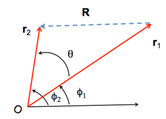
Figure 1.— Definition of the coordinate system used by observer O to point in two directions, $\mathbf{r}_{1}$ and $\mathbf{r}_{2}$, which form a plane. Here we assume $\phi_{1}\leq\phi_{2}$. Implicitly $\phi_{1}$ ($\phi_{2}$) depends on $r_{1}$ $(r_{2})$, $R$ and $\theta=\phi_{2}-\phi_{1}$. $\mathbf{R}$ is parallel to the reference axis of the $\phi$ angles.

Closed forms were established, e.g., in reference Szalay et al. (1998) when $z_{1},z_{2}\ll 1$ and without this restriction, as well as and more generally in the context of wide-angle surveys (Matsubara et al., 2000; Matsubara, 2004; Szapudi, 2004; Pápai & Szapudi, 2008; Raccanelli et al., 2010; Bertacca et al., 2012; Montanari & Durrer, 2012). Exploiting the invariance of $\xi$ with respect to the rotation of the triangle $(\mathbf{r}_{1},\mathbf{r_{2}},\mathbf{R})$, one can get an expansion on the orthogonal basis of the tripolar spherical harmonic functions defined as (Varshalovich et al., 1988; Szapudi, 2004; Pápai & Szapudi, 2008; Raccanelli et al., 2010)

$$S_{\ell_{1}\ell_{2}\ell}(\mathbf{n}_{1},\mathbf{n}_{2},\mathbf{n}_{12}) = \sum_{m_{1},m_{2},m}\begin{pmatrix}\ell_{1}&\ell_{2}&\ell\\ m_{1}&m_{2}&m\end{pmatrix}$$ (13)

$$\times C_{\ell_{1}m_{1}}(\mathbf{n}_{1})C_{\ell_{2}m_{2}}(\mathbf{n}_{2})C_{\ell m}(\mathbf{n}_{12}),$$

with the Wigner 3-j symbol in parentheses and

$$C_{\ell m}(\mathbf{n}_{12})=\sqrt{\frac{4\pi}{2\ell+1}}Y_{\ell m}(\mathbf{n}_{12}).$$

Using a specific coordinate system (Figure 1), the tripolar spherical expansion reduces to a compact form (Szapudi, 2004; Pápai & Szapudi, 2008; Montanari & Durrer, 2012)

$$\begin{split}\xi(z_{1},z_{2},\phi_{1},\phi_{2})=&G(z_{1})G(z_{2})\\ \times\sum_{m_{1}m_{2}=\ 0,1,2}&\left[a_{m_{1}m_{2}}\cos(m_{1}\phi_{1})\cos(m_{2}\phi_{2})\right.\\ &+\left.b_{m_{1}m_{2}}\sin(m_{1}\phi_{1})\sin(m_{2}\phi_{2})\right]\\ \end{split}$$ (14)

The $a_{m_{1}m_{2}}$ and $b_{m_{1}m_{2}}$ coefficients (see Appendix A) depend on

1. $f_{a}(z_{1})$, $f_{a}(z_{2})$ and

2. $\zeta_{\ell}^{m}(R)$, integral functions defined as

   $$\zeta_{\ell}^{m}(R)=\int\frac{\mathtt{d}k}{2\pi^{2}}k^{m}j_{\ell}(kR)P_{z=0}(k)$$ (15)

   with $j_{\ell}(x)$ as the spherical Bessel function of order $\ell$, and

   $$R(r_{1},r_{2},\theta)=\sqrt{r_{1}^{2}+r_{2}^{2}-2r_{1}r_{2}\cos\theta}.$$ (16)

   In the case of matter density and RSD contributions one needs to compute $\zeta_{m}^{2}(R)$ with $m=0,2,4$, exhibiting an integrand proportional to $k^{2}\ P_{z=0}(k)$.

One can define $\phi_{1}$ and $\phi_{2}$ as functions of $r_{1}$, $r_{2}$ and $\theta$ as

$$\phi_{1} = \arcsin\left(\frac{r_{2}}{R}\sin\theta\right)$$

$$\phi_{2} = \phi_{1}+\theta=\arcsin\left(\frac{r_{1}}{R}\sin\theta\right)$$ (17)

so that it is justified to consider $\xi$ as function of $(z_{1},z_{2},\theta)$.

3. Spherical harmonic space

We present now a new derivation of a closed form of the two-point correlation function using the spherical harmonic expansion of the galaxy count.

3.1. The power spectrum $C_{\ell}(z_{1},z_{2})$

At fixed redshift value $z$, the function $\Delta(\mathbf{n},z)$ (4) can be expanded using spherical harmonic functions as

$$\Delta(\mathbf{n},z)=\sum_{\ell=0}^{\infty}a_{\ell m}(z)Y_{\ell m}(\mathbf{n})$$ (18)

The $a_{\ell m}(z)$ coefficients are related to the Fourier transform of $\Delta(\mathbf{n},z)$ by the following relation:

$$a_{\ell m}(z)=i^{\ell}\sqrt{\frac{2}{\pi}}\int d\mathbf{k}\ \Delta(\mathbf{k},z)j_{\ell}(kr(z))Y^{\ast}_{\ell m}(\hat{\mathbf{k}}).$$ (19)

Using the identity (Yoo et al., 2009)

$$i\,(\hat{\mathbf{k}}.\mathbf{n})\ e^{i\ kr\ (\hat{\mathbf{k}}.\mathbf{n})}=\frac{\partial}{\partial(kr)}e^{i\ kr\ (\hat{\mathbf{k}}.\mathbf{n})}\;,$$ (20)

then the spherical harmonic contributions from the density fluctuation and the velocity gradient read

$$a_{\ell m}^{D}(z) = i^{\ell}\sqrt{\frac{2}{\pi}}\int\mathrm{d}\mathbf{k}\ D(\mathbf{k},z)j_{\ell}(kr(z))Y^{\ast}_{\ell m}(\hat{\mathbf{k}})$$

$$a_{\ell m}^{\partial V}(z) = i^{\ell}\sqrt{\frac{2}{\pi}}\int\mathrm{d}\mathbf{k}\ kV(\mathbf{k},z)j_{\ell}^{\prime\prime}(kr(z))Y^{\ast}_{\ell m}(\hat{\mathbf{k}}).$$ (21)

The $j_{\ell}^{\prime\prime}(x)$ is the second derivative of the $j_{\ell}(x)$ function. The spherical harmonics expansion of Equation (4) reads

$$\begin{split}a_{\ell m}(z)=i^{\ell}\sqrt{\frac{2}{\pi}}&\int d\mathbf{k}\Psi_{in}(\mathbf{k})T_{D}(k,z)\\ &\times\left[j_{\ell}(kr(z))-f_{a}(z)j_{\ell}^{\prime\prime}(kr(z))\right]Y^{\ast}_{\ell m}(\hat{\mathbf{k}}).\end{split}$$ (22)

The angular power spectrum $C_{\ell}(z_{1},z_{2})$ is obtained as an ensemble average of the correlation between two $a_{\ell m}(z)$

$$\begin{split}C_{\ell}(z_{1},z_{2})&=\langle a_{\ell m}(z_{1})a_{\ell m}^{\ast}(z_{2})\rangle\\ &=G(z_{1})G(z_{2})\frac{2}{\pi}\int\mathrm{d}k\ k^{2}\ P|_{z=0}(k)\\ &\times\left\{j_{\ell}(kr_{1})-f_{a}(z_{1})j_{\ell}^{\prime\prime}(kr_{1})\right\}\left\{j_{\ell}(kr_{2})-f_{a}(z_{2})j_{\ell}^{\prime\prime}(kr_{2})\right\}.\end{split}$$ (23)

where $r_{i}=r(z_{i})$.

3.2. The new $\xi$ expansion

Using the statistical isotropy of our universe, the correlation function $\xi$ may be computed by summing up the $C_{\ell}$’s (Durrer, 2008; Di Dio et al., 2013, 2014; Lepori et al., 2017) according to Equation (2). The expression of the $\xi$ function reads

$$\begin{split}\xi(\theta,&z_{1},z_{2})=G(z_{1})G(z_{2})\frac{1}{2\pi^{2}}\int\mathrm{d}k\ k^{2}P|_{z=0}(k)\\ &\times\left\{\sum_{\ell=0}^{\infty}(2\ell+1)P_{\ell}(\cos\theta)j_{\ell}(kr_{1})j_{\ell}(kr_{2})\right.\\ &-f_{a}(z_{2})\sum_{\ell=0}^{\infty}(2\ell+1)P_{\ell}(\cos\theta)j_{\ell}(kr_{1})j^{\prime\prime}_{\ell}(kr_{2})\\ &-f_{a}(z_{1})\sum_{\ell=0}^{\infty}(2\ell+1)P_{\ell}(\cos\theta)j_{\ell}(kr_{2})j^{\prime\prime}_{\ell}(kr_{1})\\ &\left.+f_{a}(z_{1})f_{a}(z_{2})\sum_{\ell=0}^{\infty}(2\ell+1)P_{\ell}(\cos\theta)j^{\prime\prime}_{\ell}(kr_{1})j^{\prime\prime}_{\ell}(kr_{2})\right\}.\end{split}$$ (24)

We define the function $A(x_{1},x_{2},\theta)$ by the following result (Abramowitz & Stegun, 1964, Equation (10.1.45))

$$\begin{split}A(x_{1},x_{2},\theta)&=\sum_{\ell=0}^{\infty}(2\ell+1)P_{\ell}(\cos\theta)j_{\ell}(x_{1})j_{\ell}(x_{2})\\ &=\textrm{sinc}(R(x_{1},x_{2},\theta))\end{split}$$ (25)

where $\mathrm{sinc}(x)=\sin(x)/x=j_{0}(x)$ and $x_{i}=kr_{i}$. It yields that the $\xi$ function can be expressed as the following expansion:

$$\begin{split}\xi(\theta,&z_{1},z_{2})=G(z_{1})G(z_{2})\frac{1}{2\pi^{2}}\int\mathrm{d}k\ k^{2}\ P|_{z=0}(k)\\ &\times\left\{A(x_{1},x_{2},\theta)-f_{a}(z_{2})\frac{\partial^{2}A(x_{1},x_{2},\theta)}{\partial x_{2}^{2}}-f_{a}(z_{1})\frac{\partial^{2}A(x_{1},x_{2},\theta)}{\partial x_{1}^{2}}\right.\\ &\left.+f_{a}(z_{1})f_{a}(z_{2})\frac{\partial^{4}A(x_{1},x_{2},\theta)}{\partial x_{1}^{2}\partial x_{2}^{2}}\right\}\end{split}$$ (26)

which establishes our main result. The $A$-function and its derivatives depend on $kr_{1}$, $kr_{2}$ and $\cos\theta$ and on the derivative of $\mathrm{sinc}(x)$ (Appendix B).

Equations (14) and (26) are two expansions that are in principle of the same $\xi$ function, and indeed in Appendix C we demonstrate formally that it is case. However, we find that our formulation is more straightforward and we provide a public implementation within the Angpow software, which will be discussed in Section 4. It also provides a natural framework to incorporate the relativistic terms, as exemplified next.

3.3. Beyond the Kaiser RSD contribution to galaxy count

So far, we have only considered the matter density fluctuation and the main RSD contributions that lead to expression (4). Durrer (2008), Yoo et al. (2009), Yoo (2010), Challinor & Lewis (2011) and Bonvin & Durrer (2011) described in detail other expressions. It is not the purpose of this section to review all of them but rather to show with two examples how expression (26) can be extended.

3.3.1 Doppler-like term

The first case concerns terms proportional to $\mathbf{V}(\mathbf{n},z).\mathbf{n}$, e.g. a sub-dominant RSD (except at low redshift), a boost term or a selection function as considered, for instance, in Pápai & Szapudi (2008); Raccanelli et al. (2010); Montanari & Durrer (2012); Di Dio et al. (2013); Raccanelli et al. (2016). The perturbation can be described with a generic $\alpha(z)$ function as

$$\Delta_{\mathbf{V.n}}(\mathbf{n},z)=-\frac{\alpha(z)}{r(z)}\mathbf{V}(\mathbf{n},z).\mathbf{n}$$ (27)

Such a contribution in Fourier space gives rise to a term proportional to $\hat{\mathbf{k}}.\mathbf{n}$

$$\Delta_{\mathbf{V.n}}(\mathbf{k},z)=i\frac{\alpha(z)}{r(z)}(\hat{\mathbf{k}}.\mathbf{n})V(\mathbf{k},z)$$ (28)

and leads to contributions to expansion (14) discussed in Montanari & Durrer (2012). However, using the identity (20), one can deduce that in spherical harmonic space it yields a contribution to Equation (22) of the form

$$\begin{split}a_{\ell m}^{\mathbf{V.n}}(z)=-i^{\ell}\sqrt{\frac{2}{\pi}}&\int d\mathbf{k}\Psi_{in}(\mathbf{k})T_{D}(k,z)Y^{\ast}_{\ell m}(\hat{\mathbf{k}})\\ &\times\frac{\alpha(z){\cal H}(z)f_{a}(z)}{kr(z)}j_{\ell}^{\prime}(kr(z))\end{split}$$ (29)

which exhibit a $j_{\ell}^{\prime}(x)$ factor. Then, correspondingly, this leads to contributions to expression (26) due to sums over $\ell$ similar to those shown in Equation (24) which may be expressed as derivatives of the $A$ function (25) as

$$\sum_{\ell=0}^{\infty}(2\ell+1)P_{\ell}(\cos\theta)j_{\ell}^{\prime}(x_{i})j^{(n)}_{\ell}(x_{j})=\frac{\partial^{n+1}A}{\partial x_{i}\partial^{n}x_{j}}$$ (30)

with $j^{(n)}_{\ell}(x)$ the $n$-th derivative of $j_{\ell}(x)$ with respect to $x$. This result can be generalized to any power of $(\hat{\mathbf{k}}.\mathbf{n})^{p}$ that is converted to a $p$-th derivative of the $A(x_{i},x_{j},\theta)$ function with respect to $x_{i}$ (and $x_{j}$).

3.3.2 Lensing term

The second case concerns integral terms as the solid angle distortion generated by gravitation lensing (e.g., Bonvin & Durrer 2011; Bonvin 2014; Montanari & Durrer 2015) which reads

$$\begin{split}\Delta_{\mathrm{lens}}(\mathbf{n},z)=-\frac{1}{r(z)}\int_{0}^{r(z)}\mathrm{d}r^{\prime}&\left(\frac{r(z)-r^{\prime}}{r^{\prime}}\right)\\ &\times\Delta_{\Omega}\left[(\Psi+\Phi)(r^{\prime}\mathbf{n},\tau_{0}-r^{\prime})\right]\end{split}$$ (31)

with $\Psi$ and $\Phi$ as the Bardeen fields (Bardeen, 1980) corresponding to the temporal and spatial metric perturbations in the longitudinal gauge, and

$$\Delta_{\Omega}\equiv\left(\cot\theta\frac{\partial}{\partial\theta}+\frac{\partial^{2}}{\partial\theta^{2}}\right)+\left(\frac{1}{\sin^{2}\theta}\frac{\partial}{\partial\phi}\right)\equiv\Delta_{\theta}+\Delta_{\phi}$$ (32)

as the angular Laplacian operator in spherical coordinates. In harmonic space, Equation (31) gives a new contribution to $a_{\ell m}(z)$ (Equation (22)), which for simplicity, can be written here using the equality between the $\Psi$ and $\Phi$ fields in linear theory in case of $\Lambda$CDM:

$$\begin{split}a_{\ell m}^{\mathrm{lens}}(z)&=i^{\ell}\ell(\ell+1)\sqrt{\frac{8}{\pi}}\int_{0}^{r(z)}\mathrm{d}r^{\prime}\left(\frac{r(z)-r^{\prime}}{r(z)r^{\prime}}\right)\\ &\times\int\mathrm{d}\mathbf{k}\ Y^{\ast}_{\ell m}(\hat{\mathbf{k}})\ \Psi(\mathbf{k},z^{\prime})j_{\ell}(kr^{\prime})\end{split}$$ (33)

where we have used the property $\Delta_{\Omega}Y^{\ast}_{\ell m}=-\ell(\ell+1)Y^{\ast}_{\ell m}$. Using the result given in Bonvin (2014), the transfer function $T_{\Psi}(k,z)$ associated with the $\Psi$ field is related to $T_{D}(k,z)$ (Equation (6)) as

$$\begin{split}\Psi(\mathbf{k},z)&=T_{\Psi}(k,z)\Psi_{\mathrm{in}}(\mathbf{k})\\ T_{\Psi}(k,z)&=-\frac{3}{2}\Omega_{m}(1+z)\left(\frac{H_{0}}{k}\right)^{2}T_{D}(k,z)\,\end{split}$$ (34)

with $\Omega_{m}$ as the present matter density parameter and $H_{0}$ as the present Hubble parameter. It yields

$$\begin{split}a_{\ell m}^{\mathrm{lens}}(z)&=i^{\ell}\ell(\ell+1)(-3\Omega_{m}H_{0}^{2})\sqrt{\frac{2}{\pi}}\\ &\times\int_{0}^{z}\frac{\mathrm{d}z^{\prime}}{H(z^{\prime})}\left(\frac{r(z)-r(z^{\prime})}{r(z)r(z^{\prime})}\right)(1+z^{\prime})\\ &\times\int\frac{\mathrm{d}\mathbf{k}}{k^{2}}\ Y^{\ast}_{\ell m}(\hat{\mathbf{k}})\ \Psi_{\mathrm{in}}(\mathbf{k})T_{D}(k,z^{\prime})j_{\ell}(kr(z^{\prime}))\end{split}$$ (35)

where we have changed the integration variable $r^{\prime}$ to $z^{\prime}$.

Combining this result with the density and RSD contributions of Equation (22) and the extension given by Equation (29), the expression of $\xi(\theta;z_{1},z_{2})$ leads to new infinite $\ell$-sums of two types:

$$S_{\mathrm{lens-cross}} = \sum_{\ell=0}^{\infty}(2\ell+1)P_{\ell}(\cos\theta)j_{\ell}^{(n)}(x)\ell(\ell+1)j_{\ell}(x^{\prime})\quad$$ (36)

$$S_{\mathrm{lens-lens}} = \sum_{\ell=0}^{\infty}(2\ell+1)P_{\ell}(\cos\theta)\ell^{2}(\ell+1)^{2}j_{\ell}(x)j_{\ell}(x^{\prime})\quad.$$ (37)

The first equation type comes from the cross-correlation of the lensing term with the density or RSD terms, as well as those concerned by the $\mathbf{V.n}$ contribution, leading to a $j_{\ell}^{(n)}(x)$ factor ($x=kr(z)$ and similarly $x^{\prime}=kr(z^{\prime})$). The second equation is the autocorrelation of the lensing term.

These two equation types can be handled with the following Legendre polynomial property

$$\Delta_{\theta}P_{\ell}(\cos\theta)=-\ell(\ell+1)P_{\ell}(\cos\theta),$$ (38)

which yields to the following derivative operator actions on the $A(x,x^{\prime},\theta)$ function:

$$\begin{split}S_{\mathrm{lens-cross}}&=-\left(\frac{\partial^{n}}{\partial x^{n}}\Delta_{\theta}\right)A(x,x^{\prime},\theta)\\ S_{\mathrm{lens-lens}}&=\left(\Delta_{\theta}^{2}\right)A(x,x^{\prime},\theta),\end{split}$$ (39)

where the $\Delta_{\theta}$ operator acts on $\theta$ in $R(x,x^{\prime},\theta)$ (see Appendix B). With these results we can include the lensing terms in the computation of $\xi(\theta,z_{1},z_{2})$ using the method developed in Section 3.

4. Implementation in Angpow

The formalism we developed is very suitable to implementation within our public code Angpow (Campagne et al., 2017), which performs fast and accurate computations of such highly oscillating integrals. The latest version now includes the computation of $\xi(\theta,z_{1},z_{2})$ with density, RSD, and Doppler terms .

In practice, we compute

$$\bar{\xi}(\theta,z_{1},z_{2})=\iint\mathrm{d}z\ \mathrm{d}z^{\prime}W_{1}(z,z_{1},\sigma_{1})W_{2}(z^{\prime},z_{2},\sigma_{2})\ \xi(\theta,z,z^{\prime})$$ (40)

with $W_{i}(z,z_{i},\sigma_{i})$ $(i=1,2)$, a user-defined redshift selection function of typical $\sigma_{i}$ width centered around $\langle z\rangle=z_{i}$ (class RadSelectBase). For this release the $\xi(\theta,z,z^{\prime})$ function includes the density, RSD contributions developed in Section 3.2, and the $\mathbf{V.n}$ (Doppler-like) contribution introduced in Section 3.3.1.

Gathering the different contributions, one can write

$$\xi(\theta,z,z^{\prime})=\frac{G(z)G(z^{\prime})}{2\pi^{2}}\int\mathrm{d}k\ k^{2}\ P|_{z=0}(k)\ f(k;\theta,z,z^{\prime})$$ (41)

with $P|_{z=0}(k)$ determined from the concrete implementation of the class PowerSpecBase to read an external $(k,P(k))$-tuple saved by the CLASSgal output. The default growth factor $G(z)$ is taken from Lahav et al. (1991) and Carroll et al. (1992), from which we compute the $f_{a}(z)$ function. The $f(k;\theta,z,z^{\prime})$ implementation reads

$$\begin{split}f(&k;\theta,z,z^{\prime})\\ &=bb^{\prime}A-bf_{a}^{\prime}\partial^{2}_{x^{\prime 2}}A-b^{\prime}f_{a}\partial^{2}_{x^{2}}A+f_{a}f_{a}^{\prime}\partial^{4}_{x^{2}x^{\prime 2}}A\\ &-b\frac{\tilde{\alpha}^{\prime}}{x^{\prime}}\,\partial_{x^{\prime}}A-b^{\prime}\frac{\tilde{\alpha}}{x}\,\partial_{x}A+\frac{\tilde{\alpha}f_{a}^{\prime}}{x}\partial^{3}_{x\,x^{\prime 2}}A\\ &+\frac{\tilde{\alpha}^{\prime}f_{a}}{x^{\prime}}\partial^{3}_{x^{2}\,x^{\prime}}A+\frac{\tilde{\alpha}\tilde{\alpha}^{\prime}}{x\,x^{\prime}}\partial^{2}_{x\,x^{\prime}}A\end{split}$$ (42)

where we have explicitly exhibited the bias $b=b(z)$ factor, $f_{a}=f_{a}(z)$, and $A$ stands for $A(\theta,x,x^{\prime})$ with $x=kr(z)$. We have contracted the notation of the $A$-function derivatives as $\partial^{n}_{x^{p}\,x^{\prime q}}A=\partial^{n}A/(\partial x^{p}\partial x^{\prime q})$, with $p+q=n$. The $\tilde{\alpha}(z)$ function is defined from $\alpha(z)$ (Equation (27)) as $\alpha(z){\cal H}(z)f_{a}(z)$. The sub-leading term of the RSD leads to $\tilde{\alpha}(z)=2f_{a}(z)$ (Montanari & Durrer, 2012). The prime stands for the $z^{\prime}$ dependence of the different terms. In Equation (42) note the density contribution autocorrelation at the first line, the density-RSD cross-correlation and RSD autocorrelation at the second line, the density-Doppler cross-correlation at the third line, the RSD-Doppler cross-correlation at the fourth line, and the Doppler autocorrelation at the last line. As an illustration, the Figure 2 shows the behaviors of the different pieces entering Equations (40-42), taking into account the density and main RSD terms, and Dirac selection functions at $z_{1}=1$ and $z_{2}$ such that $r(z_{2})-r(z_{1})=50$ Mpc, and different $\theta$ values: 0 mrad in panel (a), 20 mrad in panel (b), and 40 mrad in panel (c).

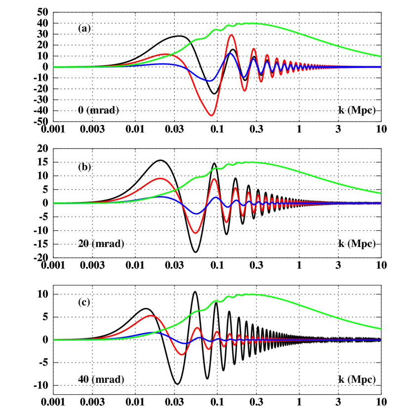
Figure 2.— Behaviors of the different contributions to the $\xi(\theta,z_{1},z_{2})$ integral described in Equations (40-42) with $z_{1}=1$, $z_{2}$ corresponding to $r(z_{2})-r(z_{1})=50$ Mpc and $\theta=$ 0 mrad in panel (a), 20 mrad in panel (b), and 40 mrad in panel (c). The matter density and the main RSD contributions and their interference are represented by black, blue, and red curves, respectively. In each panel, the $k^{2}P|_{z=0}(k)$ function is shown in green in arbitrary units from a standard $\Lambda$CDM cosmology.

The $\xi(\theta,z,z^{\prime})$ function can be computed thanks to the 3C-algorithm developed for Angpow and described in Campagne et al. (2017). In brief, this algorithm proceeds as follows:

1. the total integration $k$ interval (e.g., $[k_{\mathrm{min}},k_{\mathrm{max}}]$) in Equation (41) is cut on several $k$-sub-intervals;

2. on each sub-interval the functions

   $$f_{1}(k)=G(z)G(z^{\prime})/(2\pi^{2})\times k^{2}\ P|_{z=0}(k)$$

   and schematically

   $$f_{2}(k)=f(k;\theta,z,z^{\prime})$$

   are projected onto Chebyshev series of order $2^{N}$;

3. the product of the two Chebyshev series is performed with a $2^{2N}$ Chebyshev series;

4. then, the integral on the sub-interval is computed thanks to the Clenshaw-Curtis quadrature.

All the Chebyshev expansions and the Clenshaw-Curtis quadrature are performed via the DCT-I fast transform of FFTW.

5. Numerical results

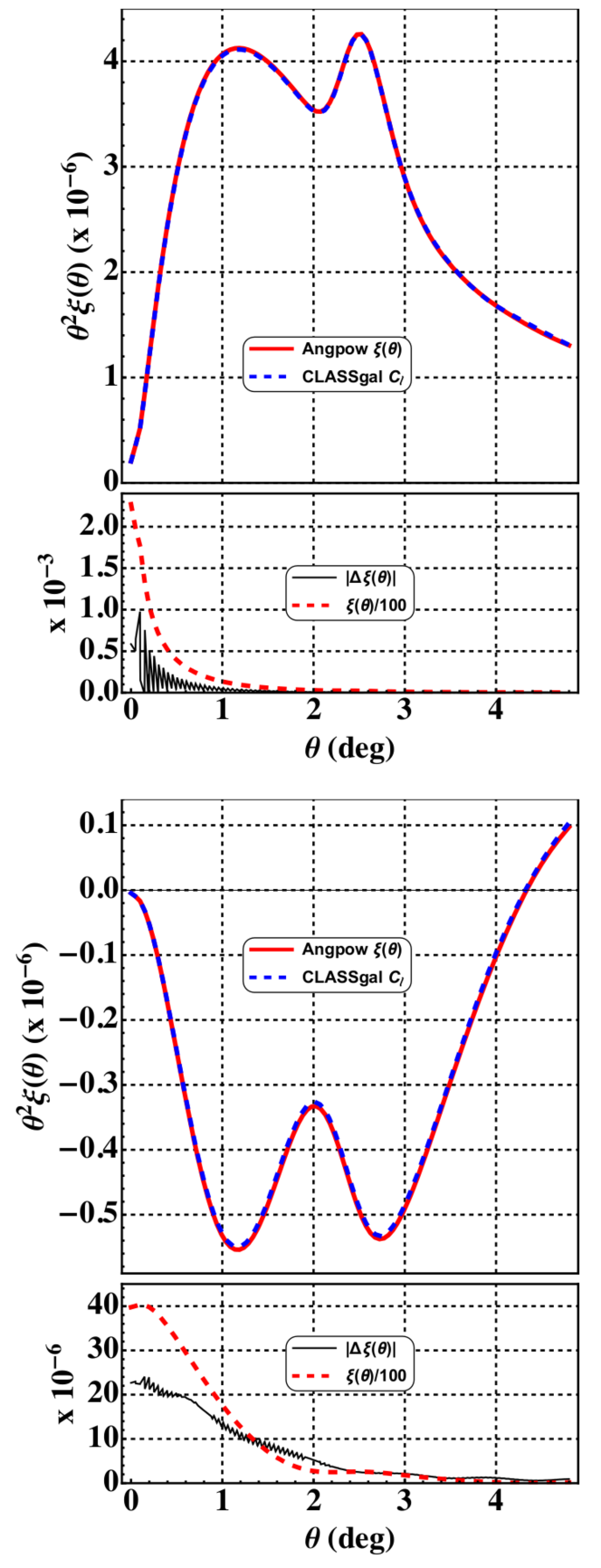
Figure 3.— Top panel: the $\theta^{2}\xi(\theta,z_{1},z_{2})$ computations with $z_{1}=z_{2}=1.00$ and a Gaussian selection function of width $\sigma=0.01$, with redshift-space distortions included. The red curve is the result of the present paper (Equations (26) and (41)), while the blue dashed curves displays the CLASSgal result given by the $C_{\ell}$ summation. Shown in the bottom panel is the absolute differences $\Delta\xi$ between the present paper and the CLASSgal results (black curve). As a matter of scale, we also display the $\xi(\theta,z_{1},z_{2})$ spectrum downscaled by a factor 100. Bottom panel(s): with the same color conventions and code parameters we display the results of the cross-correlation between two shells centered at $z_{1}=1.00$ and $z_{2}=1.05$ ($\sigma=0.01$).

To test and benchmark our $\xi$ closed form implementation, we have chosen to compare its output to the flexible, publicly and well established available software that performs similar computations, CLASSgal (Di Dio et al., 2013). Note that the CAMBsource (Challinor & Lewis, 2011) code is in principle able to perform the same computation. We have chosen a standard cosmology (for instance we set $h=0.679$, $\Omega_{\mathrm{b}}=0.0483$, $\Omega_{\mathrm{m}}=0.2582$ and $\Omega_{\mathrm{k}}=\Omega_{\mathrm{fld}}=0$). We compute with each code the density+RSD correlation functions in and between two shells at redshifts of $z_{1}=1$ and $z_{2}=1.05$, and a common Gaussian redshift selection width of $\sigma=0.01$. For a proper comparison we turned off the Limber approximations in CLASSgal. We set a cut on the $k$ integral at $k_{\texttt{max}}=1~{}\mathrm{Mpc}^{-1}$ because of memory overload with CLASSgal for larger values. In contrast our implementation is not memory-limited. Since the CLASSgal code only computes the $C_{\ell}(z_{1},z_{2})$ power spectra, afterward we perform the Equation (2) transform. We emphasize that in our formalism the $\ell$ sum in Equation (25) is performed formally up to infinity, so for comparison with a $C_{\ell}$-based approach we need to go to very high multipoles. Fortunately, any $k_{\mathtt{max}}$ cut that anyhow always exists in real survey analysis also limits the power in harmonic space to roughly $\ell_{\mathtt{max}}\simeq\langle r(z)\rangle\,k_{\mathtt{max}}$, where $\langle r(z)\rangle$ is the mean comobile distance to the shells. Since in our benchmark setup $\langle r(z)\rangle\simeq 3300$ Mpc, we compute multipoles up to $\ell_{\mathtt{max}}=3500$ and no extra apodizing smoothing is necessary to wash out the $\ell_{\mathtt{max}}$ cut effect, since the $C_{\ell}$ spectrum decreases quickly enough to 0 at $\ell=\ell_{\mathtt{max}}$.

A comparison between both computations of the correlation functions is shown in Figure 3. They agree at the percent level. The main difference is in the CPU time and Random Access Memory (RAM) used. While CLASSgal runs on 8 threads lasting around $3$ min and requires 50GB of RAM, our computation is performed in 30 s using 500 MB of RAM. On 16 threads, the wall time with CLASSgal is essentially unchanged but requires 100 GB of RAM, while our implementation runs in 18 s with 1 GB of RAM.

With such performances we can also display the full anisotropic $\xi(\theta,z_{1},z_{2})$ function in the observable space ($\theta$, $\Delta z=z_{2}-z_{1}$). With this purpose we fix $z_{1}$ to 1 and vary $\theta$ and $z_{2}$. This is similar to the figures displayed in reference Matsubara (2004), but we can show the effect of the redshift selection function. In the upper left plot of Figure 4, obtained without RSD and Dirac radial selection functions (panel (a)), one can discern the isotropic BAO wiggle corresponding to a comoving sound horizon scale of about 150 Mpc. Switching to a Gaussian redshift selection function ($\sigma=0.01$, panel (b)) stretches out the central peak along the $\Delta z$ axis (note that no angular resolution has been taken into account) and the BAO wiggle is washed out along $\theta\approx 0$, while it is preserved at higher angles for close $z$-shells ($\Delta z\approx 0)$. Turning on the RSD contributions, i.e., both the density-RSD cross-correlation and the RSD self-correlation (panel (c) for Dirac selection and panel (d) for Gaussian selection), tends to shrink the central correlation peak along the $\Delta z$ axis and to also develop a negative correlation for $\theta\approx 0$ and $\Delta z=\pm 0.05$ corresponding approximately to where the BAO peak sits in the Dirac-w/o RSD case (panel (a)). The effect of the Gaussian redshift selection function in the presence of RSD is identical that in the Dirac case.

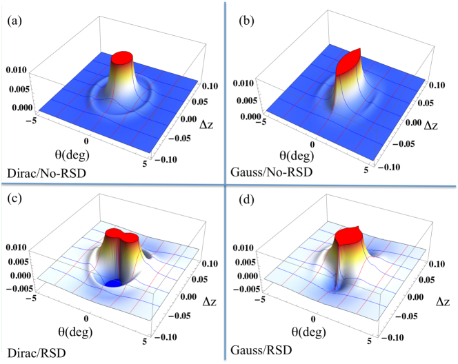
Figure 4.— Values of $\xi(\theta,z_{1},z_{2})$ presented as surface plots depending on $\theta$ and $\Delta z=z_{2}-z_{1}$ with $z_{1}=1$, using Dirac (a), (c) or Gaussian (b), (d) redshift selection functions and without (a), (b) or with (c), (d) RSD terms. For Gaussian selection we have used $\sigma=0.01$ and a $5\sigma$ cut. The color scheme is just a one-to-one correspondence of the vertical scale, but it allows one to appreciate the relief of the surface.

6. Summary and Outlooks

We have described a straightforward method to obtain a closed form for the angular correlation function of galaxy counts $\xi(\theta,z_{1},z_{2})$ (Equation (26)). The main ingredient to derive it was a reformulation of the problem in harmonic space and an addition theorem (Equation (25)), which lead to the simple analytic functions presented in Appendix B. The closed form determined with our approach has been checked to correspond to a previous one after identifying the different expansion coefficients.

The 3C-algorithm detailed in reference Campagne et al. (2017) and our compact form of $\xi(\theta,z_{1},z_{2})$ offer a fast and accurate way to compute such correlation functions. We have implemented, tested, and benchmarked it within our Angpow public code. We have presented and discussed the full angular correlation functions in 2D space involving the density-density correlation as well as the RSD-RSD and the RSD-density terms, and compare the accuracy and speed to the public code CLASSgal.

Our approach can also include other terms from the relativistic linear perturbation theory, such as the Doppler effect, which implies some simple extra derivatives, or the lensing effects, which requires the angular derivatives of the Laplacian operator.

Our code is fast enough to transform each model into configuration space and to allow us to perform some clean parameter inference as if using a Monte-Carlo Markov Chain procedure. Since it works directly in the observable space, observers are not forced any more to inject some fiducial cosmology into their large-scale structure data analyses to convert angles and redshift into distances. Data could then be independent of cosmological assumptions and be freely used to test the $\Lambda$CDM-General Relativity paradigm, which has been assumed in the derivation of the $\xi(\theta,z_{1},z_{2})$ close form expression of this work.

Appendix A $a_{m_{1}m_{2}}$ and $b_{m_{1}m_{2}}$ coefficients

Here are the expressions of the $a_{m_{1}m_{2}}$ and $b_{m_{1}m_{2}}$ coefficients used in Equation (14) from reference Montanari & Durrer (2012), where we have replaced $\beta_{i}$ by $f_{a}(z_{i})$ and $r$ by $R$ according to our definitions:

$$a_{00} = \left(1+\frac{1}{3}\left(f_{a}(z_{1})+f_{a}(z_{2})\right)+\frac{2}{15}f_{a}(z_{1})f_{a}(z_{2})\right)\zeta_{0}^{2}(R)-\left(\frac{1}{6}\left(f_{a}(z_{1})+f_{a}(z_{2})\right)+\frac{2}{21}f_{a}(z_{1})f_{a}(z_{2})\right)\zeta_{2}^{2}(R)+\frac{3}{140}f_{a}(z_{1})f_{a}(z_{2})\;\zeta_{4}^{2}(R)\;,$$

$$a_{20} = -\left(\frac{1}{2}f_{a}(z_{1})+\frac{3}{14}f_{a}(z_{1})f_{a}(z_{2})\right)\zeta_{2}^{2}(R)+\frac{1}{28}f_{a}(z_{1})f_{a}(z_{2})\;\zeta_{4}^{2}(R)\;,$$

$$a_{02} = -\left(\frac{1}{2}f_{a}(z_{2})+\frac{3}{14}f_{a}(z_{1})f_{a}(z_{2})\right)\zeta_{2}^{2}(R)+\frac{1}{28}f_{a}(z_{1})f_{a}(z_{2})\;\zeta_{4}^{2}(R)\;,$$

$$a_{22} = \frac{1}{15}f_{a}(z_{1})f_{a}(z_{2})\;\zeta_{0}^{2}(R)-\frac{1}{21}f_{a}(z_{1})f_{a}(z_{2})\;\zeta_{2}^{2}(R)+\frac{19}{140}f_{a}(z_{1})f_{a}(z_{2})\;\zeta_{4}^{2}(R)\;,$$

$$b_{22} = \frac{1}{15}f_{a}(z_{1})f_{a}(z_{2})\;\zeta_{0}^{2}(R)-\frac{1}{21}f_{a}(z_{1})f_{a}(z_{2})\;\zeta_{2}^{2}(R)-\frac{4}{35}f_{a}(z_{1})f_{a}(z_{2})\;\zeta_{4}^{2}(R)\;,$$

Appendix B Details on $R(x_{1},x_{2},\theta)$ and $A(x_{1},x_{2},\theta)$ function derivatives

In this Appendix we provide the detailed expressions for the derivative functions involved in Equation (26) and also first-order derivatives that can be used in other use cases. To stabilize the oscillation behavior of these functions, it is convenient to perform the derivation with respect to the square of the $R$ function. In the following, we define $x\equiv x_{2}-x_{1}$ and $T\equiv\theta/2$. We start with the derivatives of the $R^{2}$ function, which yield

$$\frac{\partial R^{2}}{\partial x_{1}}=-2x+4x_{2}\sin^{2}T,\qquad\frac{\partial R^{2}}{\partial x_{2}}=2x+4x_{1}\sin^{2}T,\qquad\frac{\partial^{2}R^{2}}{\partial x_{1}\partial x_{2}}=-2+4\sin^{2}T,\qquad\frac{\partial^{2}R^{2}}{\partial x_{1}^{2}}=\frac{\partial^{2}R^{2}}{\partial x_{2}^{2}}=2$$ (B1)

The higher-order derivatives with respect to $x_{1}$ or $x_{2}$ are null. Considering the derivatives of the $R$ function itself yields

$$\frac{\partial R}{\partial x_{1}} =\frac{1}{2R}\ \frac{\partial R^{2}}{\partial x_{1}} \frac{\partial R}{\partial x_{2}} =\frac{1}{2R}\ \frac{\partial R^{2}}{\partial x_{2}}$$

$$\frac{\partial^{2}R}{\partial x_{1}^{2}} =\frac{1}{4R^{3/2}}\left[-\left(\frac{\partial R^{2}}{\partial x_{1}}\right)^{2}+4R^{2}\right] \frac{\partial^{2}R}{\partial x_{2}^{2}} =\frac{1}{4R^{3/2}}\left[-\left(\frac{\partial R^{2}}{\partial x_{2}}\right)^{2}+4R^{2}\right]$$

$$\frac{\partial^{2}R}{\partial x_{1}\partial x_{2}} =\frac{1}{4R^{3/2}}\left[-\frac{\partial R^{2}}{\partial x_{1}}\frac{\partial R^{2}}{\partial x_{2}}+2R^{2}\frac{\partial^{2}R^{2}}{\partial x_{1}\partial x_{2}}\right] \frac{\partial^{3}R}{\partial x_{1}^{2}\partial x_{2}} =\frac{1}{8R^{5/2}}\left[\frac{\partial R^{2}}{\partial x_{2}}\left(3\left(\frac{\partial R^{2}}{\partial x_{1}}\right)^{2}-4R^{2}\right)-4R^{2}\frac{\partial R^{2}}{\partial x_{1}}\frac{\partial^{2}R^{2}}{\partial x_{1}\partial x_{2}}\right]$$

$$\frac{\partial^{3}R}{\partial x_{1}\partial x_{2}^{2}} =\frac{1}{8R^{5/2}}\left[\frac{\partial R^{2}}{\partial x_{1}}\left(3\left(\frac{\partial R^{2}}{\partial x_{2}}\right)^{2}-4R^{2}\right)-4R^{2}\frac{\partial R^{2}}{\partial x_{2}}\frac{\partial^{2}R^{2}}{\partial x_{1}\partial x_{2}}\right] \frac{\partial^{3}R}{\partial x_{1}\partial x_{2}^{2}} =\frac{1}{8R^{5/2}}\left[\frac{\partial R^{2}}{\partial x_{1}}\left(3\left(\frac{\partial R^{2}}{\partial x_{2}}\right)^{2}-4R^{2}\right)-4R^{2}\frac{\partial R^{2}}{\partial x_{2}}\frac{\partial^{2}R^{2}}{\partial x_{1}\partial x_{2}}\right]$$

$$\frac{\partial^{4}R}{\partial x_{1}^{2}\partial x_{2}^{2}} =\frac{1}{16R^{7/2}}\left[-15\left(\frac{\partial R^{2}}{\partial x_{1}}\right)^{2}\left(\frac{\partial R^{2}}{\partial x_{2}}\right)^{2}+12R^{2}\left\{\left(\frac{\partial R^{2}}{\partial x_{1}}\right)^{2}\right.\right.$$

$$\left.\left.+\left(\frac{\partial R^{2}}{\partial x_{2}}\right)^{2}+2\frac{\partial R^{2}}{\partial x_{1}}\frac{\partial R^{2}}{\partial x_{2}}\frac{\partial^{2}R^{2}}{\partial x_{1}\partial x_{2}}\right\}-8R^{4}\left\{2+\left(\frac{\partial^{2}R^{2}}{\partial x_{1}\partial x_{2}}\right)^{2}\right\}\right]$$ (B2)

For the sake of completeness, the derivatives of $\mathrm{sinc}(x)=j_{0}(x)$ using $\cos(x)$ and $\mathrm{sinc}(x)$ functions read

$$\mathrm{sinc}^{(1)}(x) =\frac{1}{x}\left(\cos x-\ \mathrm{sinc}\ x\right), \mathrm{sinc}^{(2)}(x) =-\frac{1}{x^{2}}\left(2\cos x+(x^{2}-2)\ \mathrm{sinc}\ x\right)$$

$$\mathrm{sinc}^{(3)}(x) =\frac{1}{x^{3}}\left(-(x^{2}-6)\cos x+3(x^{2}-2)\ \mathrm{sinc}\ x\right), \mathrm{sinc}^{(4)}(x) =\frac{1}{x^{4}}\left(4(x^{2}-6)\cos x+(x^{4}-12x^{2}+24)\ \mathrm{sinc}\ x\right)$$ (B3)

Note that the Taylor expansions at $x=0$ of these derivative functions are

$$\mathrm{sinc}^{(1)}(x) \approx-\frac{1}{3}x+\frac{1}{30}x^{3}-\frac{1}{840}x^{5}+\dots, \mathrm{sinc}^{(2)}(x) \approx-\frac{1}{3}+\frac{1}{10}x^{2}-\frac{1}{168}x^{4}+\dots$$

$$\mathrm{sinc}^{(3)}(x) \approx\frac{1}{5}x-\frac{1}{42}x^{3}+\frac{1}{1080}x^{5}+\dots, \mathrm{sinc}^{(4)}(x) \approx\frac{1}{5}-\frac{1}{14}x^{2}+\frac{1}{216}x^{4}+\dots$$ (B4)

Using the above results, the expressions of the $A$-function derivatives used in Equation (26) and also used in case to add $j^{\prime}(x)$ contributions to Equation (30), are

$$\frac{\partial A}{\partial x_{1}} =\mathrm{sinc}^{(1)}(R)\frac{\partial R}{\partial x_{1}}, \frac{\partial A}{\partial x_{2}} =\left.\frac{\partial A}{\partial x_{1}}\right|_{x_{1}\rightarrow x_{2}}$$

$$\frac{\partial^{2}A}{\partial x_{1}^{2}} =\mathrm{sinc}^{(2)}(R)\left(\frac{\partial R}{\partial x_{1}}\right)^{2}+\mathrm{sinc}^{(1)}(R)\frac{\partial^{2}R}{\partial x_{1}^{2}}, \frac{\partial^{2}A}{\partial x_{2}^{2}} =\left.\frac{\partial^{2}A}{\partial x_{1}^{2}}\right|_{x_{1}\rightarrow x_{2}}$$

$$\frac{\partial^{2}A}{\partial x_{1}\partial x_{2}} =\mathrm{sinc}^{(2)}(R)\frac{\partial R}{\partial x_{1}}\frac{\partial R}{\partial x_{2}}+\mathrm{sinc}^{(1)}(R)\frac{\partial^{2}R}{\partial x_{1}\partial x_{2}}, \frac{\partial^{3}A}{\partial x_{1}\partial x_{2}^{2}} =\frac{\partial R}{\partial x_{1}}\left\{\mathrm{sinc}^{(3)}(R)\left(\frac{\partial R}{\partial x_{2}}\right)^{2}+\mathrm{sinc}^{(2)}(R)\frac{\partial^{2}R}{\partial x_{2}^{2}}\right\}$$

$$+2\ \mathrm{sinc}^{(2)}(R)\frac{\partial R}{\partial x_{2}}\frac{\partial^{2}R}{\partial x_{1}\partial x_{2}}+\mathrm{sinc}^{(2)}(R)\frac{\partial^{3}R}{\partial x_{1}\partial x_{2}^{2}}$$

$$\frac{\partial^{3}A}{\partial x_{1}^{2}\partial x_{2}} =\left.\frac{\partial^{3}A}{\partial x_{1}\partial x_{2}^{2}}\right|_{x_{1}\rightarrow x_{2}}, \frac{\partial^{4}A}{\partial x_{1}^{2}\partial x_{2}^{2}} =\mathrm{sinc}^{(4)}(R)\left(\frac{\partial R}{\partial x_{1}}\right)^{2}\left(\frac{\partial R}{\partial x_{2}}\right)^{2}$$

$$+\mathrm{sinc}^{(3)}(R)\left\{\left(\frac{\partial R}{\partial x_{1}}\right)^{2}\frac{\partial^{2}R}{\partial x_{2}^{2}}+4\frac{\partial R}{\partial x_{1}}\frac{\partial R}{\partial x_{2}}\frac{\partial^{2}R}{\partial x_{1}\partial x_{2}}+\left(\frac{\partial R}{\partial x_{2}}\right)^{2}\frac{\partial^{2}R}{\partial x_{1}^{2}}\right\}$$

$$+\mathrm{sinc}^{(2)}(R)\left\{2\left(\frac{\partial^{2}R}{\partial x_{1}\partial x_{2}}\right)^{2}+2\frac{\partial R}{\partial x_{1}}\frac{\partial^{3}R}{\partial x_{1}\partial x_{2}^{2}}+\frac{\partial^{2}R}{\partial x_{1}^{2}}\frac{\partial^{2}R}{\partial x_{2}^{2}}\right.$$

$$\left.+2\frac{\partial R}{\partial x_{2}}\frac{\partial^{3}R}{\partial x_{1}^{2}\partial x_{2}}\right\}+\mathrm{sinc}^{(1)}(R)\frac{\partial^{4}R}{\partial x_{1}^{2}\partial x_{2}^{2}}$$ (B5)

The $\Delta_{\theta}$ operator action on the $A$-function involved in the lensing term (Section 3.3) reads

$$\begin{split}\Delta_{\theta}(A(x_{1},x_{2},\theta))&=\left(\cot\theta\frac{\partial R}{\partial\theta}+\frac{\partial^{2}R}{\partial\theta^{2}}\right)\mathrm{sinc}^{(1)}(R)+\left(\frac{\partial R}{\partial\theta}\right)^{2}\mathrm{sinc}^{(2)}(R)\\ \Delta_{\theta}^{2}(A(x_{1},x_{2},\theta))&=\left(\cot\theta\csc^{2}\theta\frac{\partial R}{\partial\theta}-(1+\csc^{2}\theta)\frac{\partial^{2}R}{\partial\theta^{2}}+2\cot\theta\frac{\partial^{3}R}{\partial\theta^{3}}+\frac{\partial^{4}R}{\partial\theta^{4}}\right)\mathrm{sinc}^{(1)}(R)\\ &+\left(-(1+\csc^{2}\theta)\left(\frac{\partial R}{\partial\theta}\right)^{2}+3\left(\frac{\partial^{2}R}{\partial\theta^{2}}\right)^{2}+\frac{\partial R}{\partial\theta}\left[6\cot\theta\frac{\partial^{2}R}{\partial\theta^{2}}+4\frac{\partial^{3}R}{\partial\theta^{3}}\right]\right)\mathrm{sinc}^{(2)}(R)\\ &+2\left(\cot\theta\frac{\partial R}{\partial\theta}+3\frac{\partial^{2}R}{\partial\theta^{2}}\right)\left(\frac{\partial R}{\partial\theta}\right)^{2}\mathrm{sinc}^{(3)}(R)\\ &+\left(\frac{\partial R}{\partial\theta}\right)^{4}\mathrm{sinc}^{(4)}(R)\end{split}$$ (B6)

with the derivatives of the $R(x_{1},x_{2},\theta)$ function with respect to $\theta$

$$\begin{split}R\frac{\partial R}{\partial\theta}&=4x_{1}x_{2}\cos\theta\sin\theta\\ R^{3}\frac{\partial^{2}R}{\partial\theta^{2}}&=2x_{1}x_{2}\left(2(x_{1}+x_{2})^{2}\cos 2\theta-x_{1}x_{2}(3+\cos 4\theta)\right)\\ R^{5}\frac{\partial^{3}R}{\partial\theta^{3}}&=-4x_{1}x_{2}\sin 2\theta\left(2(x_{1}^{4}+x_{2}^{4})+8x_{1}x_{2}(x_{1}^{2}+x_{2}^{2})+7x_{1}^{2}x_{2}^{2}+x_{1}x_{2}(x_{1}x_{2}\cos 4\theta-2\cos 2\theta\,(x_{1}+x_{2})^{2})\right)\\ R^{7}\frac{\partial^{4}R}{\partial\theta^{4}}&=-2x_{1}x_{2}\left(4\left(x_{1}+x_{2}\right){}^{2}\left(2x_{1}^{4}+8x_{1}^{3}x_{2}+11x_{1}^{2}x_{2}^{2}+8x_{1}x_{2}^{3}+2x_{2}^{4}\right)\cos 2\theta\right.\\ &+\left.x_{1}x_{2}\left(4\left(x_{1}^{4}+4x_{1}^{3}x_{2}-5x_{1}^{2}x_{2}^{2}+4x_{1}x_{2}^{3}+x_{2}^{4}\right)\cos 4\theta-7\left(4x_{1}^{4}+16x_{1}^{3}x_{2}+13x_{1}^{2}x_{2}^{2}+16x_{1}x_{2}^{3}+4x_{2}^{4}\right)\right.\right.\\ &+\left.\left.x_{1}x_{2}\left(-x_{1}x_{2}\cos 8\theta+4\left(x_{1}+x_{2}\right){}^{2}\cos 6\theta\right)\right)\right)\end{split}$$ (B7)

Appendix C Equality between the tripolar and harmonic result

We demonstrate here that both approaches in Sections 2.2 and 3.2 lead to equivalent results, although in different forms. We take Equation (26) as the initial expansion and identify the coefficients proportional to $f_{a}(z_{1})$ ($f_{a}(z_{2}))$ and $f_{a}(z_{1})f_{a}(z_{2})$. Note that the first term of expression (26) is easily identified as the $a_{00}$ one in the expression (14) just simply because $A(x_{1},x_{2},\theta)=j_{0}(kR)$, as a result of Equation (25) (note that $x_{i}=kr_{i}$). Thus, using a symbolic algebra package we can show that the term proportional to $f_{a}(z_{1})$ can be expanded as

$$\frac{\partial^{2}A}{\partial x_{1}^{2}}=-\frac{1}{3}j_{0}(kR)+\frac{1}{6}j_{2}(kR)+\frac{1}{2}j_{2}(kR)\cos 2\phi_{1}$$ (C1)

One identifies the corresponding factors of $a_{00}$ and $a_{20}$ thanks to the minus sign of Equation (26), as the $\zeta_{\ell}^{2}$ expansion can be interpreted as $j_{\ell}$ expansion. By the same method one can identify at which $a_{00}$ and $a_{20}$ factors correspond to $\partial^{2}A/\partial x_{2}^{2}$.

To get the corresponding $j_{\ell}$ expansion of the $\partial^{4}A/\partial x_{1}^{2}\partial x_{2}^{2}$ term (B5) we use the following identities:

$$\begin{split}\left(\frac{\partial R}{\partial x_{1}}\right)^{2}\left(\frac{\partial R}{\partial x_{2}}\right)^{2}&=\frac{1}{4}\left(\vphantom{\frac{1}{4}}1+\cos 2\phi_{1}\right)\left(\vphantom{\frac{1}{4}}1+\cos 2\phi_{2}\right)\\ (kR)\left\{\left(\frac{\partial R}{\partial x_{1}}\right)^{2}\frac{\partial^{2}R}{\partial x_{2}^{2}}+4\frac{\partial R}{\partial x_{1}}\frac{\partial R}{\partial x_{2}}\frac{\partial^{2}R}{\partial x_{1}\partial x_{2}}+\left(\frac{\partial R}{\partial x_{2}}\right)^{2}\frac{\partial^{2}R}{\partial x_{1}^{2}}\right\}&=\frac{1}{2}\left(\vphantom{\frac{1}{2}}1-\cos 2\phi_{1}\cos 2\phi_{2}+2\sin 2\phi_{1}\sin 2\phi_{2}\right)\\ (kR)^{2}\left\{2\left(\frac{\partial^{2}R}{\partial x_{1}\partial x_{2}}\right)^{2}+2\frac{\partial R}{\partial x_{1}}\frac{\partial^{3}R}{\partial x_{1}\partial x_{2}^{2}}+\frac{\partial^{2}R}{\partial x_{1}^{2}}\frac{\partial^{2}R}{\partial x_{2}^{2}}+2\frac{\partial R}{\partial x_{2}}\frac{\partial^{3}R}{\partial x_{1}^{2}\partial x_{2}}\right\}&=-\frac{1}{4}\left(\vphantom{\frac{1}{4}}1+3(\cos 2\phi_{1}+\cos 2\phi_{2})-7\cos 2\phi_{1}\cos 2\phi_{2}\right.\\ &\phantom{-\frac{1}{4}\left(1+3(\cos 2\phi_{1}+\cos 2\phi_{2})-\right.}\left.\vphantom{\frac{1}{4}}+8\sin 2\phi_{1}\sin 2\phi_{2}\right)\\ &=-(kR)^{3}\frac{\partial^{4}R}{\partial x_{1}^{2}\partial x_{2}^{2}}\end{split}$$ (C2)

while the derivatives of the $\mathrm{sinc}(x)$ can be expanded as a linear combination of $j_{\ell}(x)$ with $\ell=0,2,4$ according to:

$$\begin{split}\mathrm{sinc}^{(4)}(x)&=\frac{1}{5}j_{0}(x)-\frac{4}{7}j_{2}(x)+\frac{8}{35}j_{4}(x)\\ \frac{\mathrm{sinc}^{(3)}(x)}{x}&=\frac{1}{5}j_{0}(x)+\frac{1}{7}j_{2}(x)-\frac{2}{35}j_{4}(x)\\ -\frac{\mathrm{sinc}^{(1)}(x)}{x^{3}}+\frac{\mathrm{sinc}^{(2)}(x)}{x^{2}}&=\frac{1}{15}j_{0}(x)+\frac{2}{21}j_{2}(x)+\frac{1}{35}j_{4}(x).\end{split}$$ (C3)

Then, gathering the different $j_{\ell}$ factors of the combination of Equations (C2) and (C3), we recover the contributions to $a_{00}$, $a_{20}$, $a_{02}$, $a_{22}$, and $b_{22}$. So, we find that the Equations (14) and (26) match perfectly, as expected.

References

• Abramowitz & Stegun (1964) Abramowitz, M., & Stegun, I. A. 1964, Handbook of Mathematical Functions with Formulas, Graphs, and Mathematical Tables, ninth dover printing, tenth gpo printing edn. (New York: Dover)
• Bardeen (1980) Bardeen, J. M. 1980, Phys. Rev. D, 22, 1882
• Bertacca et al. (2012) Bertacca, D., Maartens, R., Raccanelli, A., & Clarkson, C. 2012, J. Cosmology Astropart. Phys, 10, 025
• Bonvin (2014) Bonvin, C. 2014, Classical and Quantum Gravity, 31, 234002
• Bonvin & Durrer (2011) Bonvin, C., & Durrer, R. 2011, Phys. Rev. D, 84, 063505
• Bonvin et al. (2014) Bonvin, C., Hui, L., & Gaztañaga, E. 2014, Phys. Rev. D, 89, 083535
• Campagne et al. (2017) Campagne, J.-E., Neveu, J., & Plaszczynski, S. 2017, to be published to A&A, arXiv:1701.03592
• Carroll et al. (1992) Carroll, S. M., Press, W. H., & Turner, E. L. 1992, ARA&A, 30, 499
• Challinor & Lewis (2011) Challinor, A., & Lewis, A. 2011, Phys. Rev. D, 84, 043516
• Di Dio et al. (2014) Di Dio, E., Montanari, F., Durrer, R., & Lesgourgues, J. 2014, J. Cosmology Astropart. Phys, 1, 042
• Di Dio et al. (2013) Di Dio, E., Montanari, F., Lesgourgues, J., & Durrer, R. 2013, J. Cosmology Astropart. Phys, 11, 044
• Durrer (2008) Durrer, R. 2008, The Cosmic Microwave Background (Cambridge University Press)
• Ivezic et al. (2008) Ivezic, Z., Tyson, J. A., Abel, B., et al. 2008, ArXiv e-prints, arXiv:0805.2366
• Kaiser (1987) Kaiser, N. 1987, MNRAS, 227, 1
• Lahav et al. (1991) Lahav, O., Lilje, P. B., Primack, J. R., & Rees, M. J. 1991, MNRAS, 251, 128
• Laureijs et al. (2011) Laureijs, R., Amiaux, J., Arduini, S., et al. 2011, ArXiv e-prints, arXiv:1110.3193
• Lepori et al. (2017) Lepori, F., Di Dio, E., Viel, M., Baccigalupi, C., & Durrer, R. 2017, J. Cosmology Astropart. Phys, 2, 020
• Levi et al. (2013) Levi, M., Bebek, C., Beers, T., et al. 2013, ArXiv e-prints, arXiv:1308.0847
• Matsubara (2004) Matsubara, T. 2004, ApJ, 615, 573
• Matsubara et al. (2000) Matsubara, T., Szalay, A. S., & Landy, S. D. 2000, ApJ, 535, L1
• Montanari & Durrer (2012) Montanari, F., & Durrer, R. 2012, Phys. Rev. D, 86, 063503
• Montanari & Durrer (2015) —. 2015, J. Cosmology Astropart. Phys, 10, 070
• Pápai & Szapudi (2008) Pápai, P., & Szapudi, I. 2008, MNRAS, 389, 292
• Raccanelli et al. (2016) Raccanelli, A., Bertacca, D., Jeong, D., Neyrinck, M. C., & Szalay, A. S. 2016, ArXiv e-prints, arXiv:1602.03186
• Raccanelli et al. (2010) Raccanelli, A., Samushia, L., & Percival, W. J. 2010, MNRAS, 409, 1525
• Szalay et al. (1998) Szalay, A. S., Matsubara, T., & Landy, S. D. 1998, ApJ, 498, L1
• Szapudi (2004) Szapudi, I. 2004, ApJ, 614, 51
• Varshalovich et al. (1988) Varshalovich, D. A., Moskalev, A. N., & Khersonsky, V. K. 1988, Quantum Theory of Angular Momentum: Irreducible Tensors, Spherical Harmonics, Vector Coupling Coefficients, 3nj Symbols (Singapore: World Scientific)
• Yoo (2010) Yoo, J. 2010, Phys. Rev. D, 82, 083508
• Yoo et al. (2009) Yoo, J., Fitzpatrick, A. L., & Zaldarriaga, M. 2009, Phys. Rev. D, 80, 083514