Kohn–Sham decomposition in real-time time-dependent density-functional theory:
An efficient tool for analyzing plasmonic excitations

Abstract

The real-time-propagation formulation of time-dependent density-functional theory (RT-TDDFT) is an efficient method for modeling the optical response of molecules and nanoparticles. Compared to the widely adopted linear-response TDDFT approaches based on, e.g., the Casida equations, RT-TDDFT appears, however, lacking efficient analysis methods. This applies in particular to a decomposition of the response in the basis of the underlying single-electron states. In this work, we overcome this limitation by developing an analysis method for obtaining the Kohn–Sham electron-hole decomposition in RT-TDDFT. We demonstrate the equivalence between the developed method and the Casida approach by a benchmark on small benzene derivatives. Then, we use the method for analyzing the plasmonic response of icosahedral silver nanoparticles up to Ag₅₆₁. Based on the analysis, we conclude that in small nanoparticles individual single-electron transitions can split the plasmon into multiple resonances due to strong single-electron–plasmon coupling whereas in larger nanoparticles a distinct plasmon resonance is formed.

I Introduction

Time-dependent density-functional theory (TDDFT) Runge and Gross (1984) built on top of Kohn–Sham (KS) density-functional theory (DFT) Hohenberg and Kohn (1964); Kohn and Sham (1965) is a powerful tool in computational physics and chemistry for accessing the optical properties of matter. Marques et al. (2012); Ullrich (2012) Starting from seminal works on jellium nanoparticles, Ekardt (1984); Puska et al. (1985); Beck (1987) TDDFT has become a standard tool for modeling plasmonic response from a quantum-mechanical perspective, Morton et al. (2011); Varas et al. (2016) and proven to be useful for calculating the response of individual nanoparticles, Prodan et al. (2003); Aikens et al. (2008); Zuloaga et al. (2010); Weissker and Mottet (2011); Li et al. (2013); Piccini et al. (2013); Burgess and Keast (2014); Barcaro et al. (2014); Weissker and Lopez-Lozano (2015); Bae and Aikens (2015); Zapata Herrera et al. (2016) and their compounds Zuloaga et al. (2009); Song et al. (2011, 2012); Marinica et al. (2012); Zhang et al. (2014); Varas et al. (2015); Barbry et al. (2015); Kulkarni and Manjavacas (2015); Rossi et al. (2015a); Marchesin et al. (2016); Lahtinen et al. (2016) as well as other plasmonic materials. Manjavacas et al. (2013); Andersen and Thygesen (2013); Andersen et al. (2014); Lauchner et al. (2015) Additionally, a number of models and concepts have been developed for quantifying and understanding plasmonic character within the TDDFT framework. Gao and Yuan (2005); Yan et al. (2007); Bernadotte et al. (2013); Malola et al. (2013); Guidez and Aikens (2012, 2014); Yasuike et al. (2011); Casanova et al. (2016); Townsend and Bryant (2012, 2014); Ma et al. (2015); Bursi et al. (2016) Thus, in conjunction with other theoretical and computational methods Esteban et al. (2012); Stella et al. (2013); Chen et al. (2015); Yan et al. (2015); Teperik et al. (2016); Ciracì and Della Sala (2016); David et al. (2016); Christensen et al. and experimental developments, Ciracì et al. (2012); Scholl et al. (2012); Haberland (2013); Savage et al. (2012); Banik et al. (2012, 2013); Scholl et al. (2013); Tan et al. (2014); Zhang et al. (2016); Sanders et al. (2016); Mertens et al. (2016) TDDFT is a valuable tool for understanding quantum effects within the nanoplasmonics field. Tame et al. (2013); Zhu et al. (2016) Recent methodological advances and a steady increase in computational power have extended the system size that can be treated at the TDDFT level, enabling the computational modeling of plasmonic phenomena in noble metal nanoparticles of several nanometers in diameter. Iida et al. (2014); Kuisma et al. (2015); Baseggio et al. (2015, 2016); Koval et al. (2016)

TDDFT in the linear-response regime is usually formulated in frequency space Casida (1995); Petersilka et al. (1996) in terms of the Casida matrix expressed in the Kohn–Sham electron-hole space. Casida (1995, 2009) The calculations are commonly performed by diagonalizing the Casida matrix directly or by solving the equivalent problem with different iterative subspace algorithms. Bauernschmitt and Ahlrichs (1996); Stratmann et al. (1998); Walker et al. (2006); Andrade et al. (2007) The real-time-propagation formulation of TDDFT (RT-TDDFT) Yabana and Bertsch (1996); Yabana et al. (2006) is a computationally efficient alternative to frequency-space approaches with favorable scaling with respect to system size, Sander and Kresse (2017) and has the additional advantage of being also applicable to the non-linear regime. However, RT-TDDFT results are often limited to absorption spectra or to analyses of transition densities, apart from a few exceptions focusing on characterizing plasmonic Townsend and Bryant (2012, 2014); Ma et al. (2015); Yan et al. (2016) or other electronic excitations. Li and Ullrich (2011, 2015); Repisky et al. (2015); Kolesov et al. (2016) In contrast, the Casida approach directly enables an extensive analysis in terms of the KS electron-hole decomposition of the excitations and thereby readily yields quantum-mechanical understanding of the plasmonic response. Yasuike et al. (2011); Guidez and Aikens (2012, 2014); Bernadotte et al. (2013); Malola et al. (2013, 2014, 2015); Baseggio et al. (2015, 2016); Casanova et al. (2016)

In this work, we remedy the lack of analysis tools in RT-TDDFT and demonstrate that the decomposition of the electronic excitations in terms of the underlying KS electron-hole space can be obtained within RT-TDDFT, in equivalent fashion to the Casida approach. We have combined the analysis method with a recent RT-TDDFT implementation Kuisma et al. (2015) based on the linear combination of atomic orbitals (LCAO) method Larsen et al. (2009) that is part of the open source gpaw code. Mortensen et al. (2005); Enkovaara et al. (2010); GPA

By using the developed method, we perform a KS decomposition analysis of the plasmon formation in a series of icosahedral silver nanoparticles comprising Ag55, Ag147, Ag309, and Ag561. We observe that while in Ag147 and larger nanoparticles a distinct plasmon resonance is formed from the superposition of single-electron transitions, in the small Ag55 nanoparticle individual single-electron transitions still have a strong effect on the plasmonic response and cause the splitting of the plasmon resonance.

The structure of the article is as follows. In Sec. II we derive the linear response of the time-dependent density matrix in the KS electron-hole space. We review the formulation of the same quantity in the Casida approach and describe the decomposition of the photo-absorption spectrum in KS electron-hole contributions. In Sec. III we benchmark the numerical accuracy of the implemented method by analyzing the KS decomposition of small benzene derivatives using both the real-time-propagation and the Casida method. This is followed by an analysis of the plasmonic response of large silver nanoparticles, which yields microscopic insight into the plasmon formation in nanoparticles. In Sec. IV we discuss the general features of the presented methodology. Our work is concluded in Sec. V.

II Methods

II.1 Linear response of the density matrix in the real-time propagation method

The time-dependent Kohn–Sham equation is defined as

$$i\frac{\partial}{\partial t}\psi_{n}(\boldsymbol{r},t)=H_{\text{KS}}(t)\psi_{n}(\boldsymbol{r},t),$$ (1)

where $H_{\text{KS}}(t)$ is the time-dependent KS Hamiltonian and $\psi_{n}(\boldsymbol{r},t)$ is a KS wave function. The density matrix operator is defined as

$$\rho(t)=\sum_{n}\ket{\psi_{n}(t)}f_{n}\bra{\psi_{n}(t)},$$ (2)

where $f_{n}$ is an occupation factor of the $n$th KS state. In order to proceed with KS decomposition, we express the density matrix in the KS basis, spanned by the ground-state KS orbitals $\psi_{n}^{(0)}(\boldsymbol{r})$, which fulfill the ground-state KS equation

$$H_{\text{KS}}^{(0)}\psi_{n}^{(0)}(\boldsymbol{r})=\epsilon_{n}\psi_{n}^{(0)}(\boldsymbol{r}),$$ (3)

where $H_{\text{KS}}^{(0)}$ is the ground-state KS Hamiltonian and $\epsilon_{n}$ the KS eigenvalue of $n$th state. The density matrix can be written in this KS basis as

$$\rho_{nn^{\prime}}(t) =\braket{\psi^{(0)}_{n}}{\rho(t)}{\psi^{(0)}_{n^{\prime}}}$$

$$=\sum_{m}\braket{\psi^{(0)}_{n}}{\psi_{m}(t)}f_{m}\braket{\psi_{m}(t)}{\psi^{(0)}_{n^{\prime}}}.$$ (4)

This equation establishes a link between a time-dependent density matrix and the usual KS (electron-hole) basis set used in linear-response calculations, see Sec. II.2. Previously, similar or related quantities have been used within the real-time propagation method for analysing the response. Li and Ullrich (2011, 2015); Townsend and Bryant (2012, 2014); Ma et al. (2015); Repisky et al. (2015); Yan et al. (2016)

When the real-time propagation method is applied in the linear-response regime, the usual approach is to use a $\delta$-pulse perturbation. Yabana and Bertsch (1996); Yabana et al. (2006) This corresponds to the Hamiltonian

$$H_{\text{KS}}(t)=H^{(0)}_{\text{KS}}+zK_{z}\delta(t),$$ (5)

where the interaction with external electromagnetic radiation is taken within the dipole approximation. The electric field is assumed to be aligned along the $z$ direction and the constant $K_{z}$ is proportional to the external electric field strength, which is assumed to be small enough to induce only negligible non-linear effects. After the perturbation by the $\delta$-pulse at $t=0$, Eq. (1) is propagated in time and the quantities of interest are recorded during the propagation. As a post-processing step time-domain quantities, e.g., $\rho_{nn^{\prime}}(t)$, can be Fourier transformed into the frequency domain.

It is important to note that the size of the density matrix $\rho_{nn^{\prime}}(t)$ can be significantly reduced since only its electron-hole part is required in linear-response theory. Casida (1995, 2009) It is thus sufficient to consider only $\rho_{ia}(t)$, where $i$ and $a$ represent occupied and unoccupied KS states, respectively. Then, we obtain the linear-response of the density matrix in electron-hole space as

$$\delta\rho^{z}_{ia}(\omega)=\frac{1}{K_{z}}\int_{0}^{\infty}\left[\rho^{z}_{ia}(t)-\rho_{ia}(0^{-})\right]e^{i\omega t}\text{d}t+\mathcal{O}(K_{z}),$$ (6)

where $\rho_{ia}(0^{-})$ is the initial density matrix before the $\delta$-pulse perturbation and the superscript $z$ indicates the direction of the perturbation.

In common TDDFT implementations, there is no mechanism for energy dissipation and the lifetime of excitations is infinite. A customary way to restore a finite lifetime is to apply the substitution $\omega\to\omega+i\eta$, where the parameter $\eta$ is small. This leads to an exponentially decaying term in the integrand in Eq. (6), i.e., $e^{i\omega t}\to e^{i\omega t}e^{-\eta t}$, and to the Lorentzian line shapes in the frequency domain. The decaying integrand also means that a finite propagation time is sufficient in practical calculations. The Gaussian line shapes can be obtained by replacing the Lorentzian decay $e^{-\eta t}$ with the Gaussian decay function $e^{-(\sigma t)^{2}/2}$, where the parameter $\sigma$ determines the spectral line width.

Implementation

We have implemented the density matrix formalism outlined above in the RT-TDDFT code Kuisma et al. (2015) that is part of the open source gpaw package Mortensen et al. (2005); Enkovaara et al. (2010); GPA . Our implementation uses the LCAO basis setLarsen et al. (2009) and the projector-augmented wave (PAW) Blöchl (1994) method. In the LCAO method the wave function $\psi_{n}(\boldsymbol{r},t)$ is expanded in localized basis functions $\phi_{\mu}(\boldsymbol{r})$ centered at atomic coordinates

$$\psi_{n}(\boldsymbol{r},t)=\sum_{\mu}\phi_{\mu}(\boldsymbol{r})C_{\mu n}(t)$$ (7)

with expansion coefficients $C_{\mu n}(t)$. The density matrix is reads in the LCAO basis set as

$$\rho_{\mu\nu}(t)=\sum_{n}C_{\mu n}(t)f_{n}C_{\nu n}^{*}(t).$$ (8)

Then, Eq. (4) can be written in LCAO formalism as (using implied summation over repeated indices)

$$\rho_{nn^{\prime}}(t)=C^{(0)*}_{\mu n}S_{\mu\mu^{\prime}}\rho_{\mu^{\prime}\nu^{\prime}}(t)S^{*}_{\nu\nu^{\prime}}C^{(0)}_{\nu n^{\prime}},$$ (9)

where $S_{\mu\mu^{\prime}}=\int\phi^{*}_{\mu}(\boldsymbol{r})\phi_{\mu^{\prime}}(\boldsymbol{r})\text{d}\boldsymbol{r}$ is the overlap integral of the basis functions. A detailed derivation of Eq. (9) is given in Appendix, in which it is shown that the PAW transformation affects only the evaluation of the overlap integral.

The emphasis in our implementation is to minimize the computational footprint of the analysis methods. Thus, instead of calculating Eq. (9) at every time step during the time propagation, we only store the already-calculated matrix $C^{z}_{\mu n}(t)$ at every time step. Then, as a post-processing step, we calculate $\rho^{z}_{\mu\nu}(t)$ with Eq. (8) and Fourier transform the result to obtain $\delta\rho^{z}_{\mu\nu}(\omega)$. The latter quantity can be subsequently transformed to $\delta\rho^{z}_{ia}(\omega)$ via Eq. (9) keeping only the electron-hole part. Thus, in practical implementation, the linearity of the equations allows exchanging the order of Fourier transformation and matrix multiplications.

Finally, we note that in our experience it is advantageous to store the whole time-dependent evolution of the system, i.e., $C^{z}_{\mu n}(t)$, as done in the present implementation. While alternative on-the-fly Fourier or other transformations would reduce the amount of required storage space, they would restrict the analysis to the set of parameters specified at the outset of the calculation.

II.2 Linear response of the density matrix in the Casida method

In Casida’s linear-response formulation of TDDFT Casida (1995, 2009) the response is obtained by solving the matrix eigenvalue equation

$${\bf\Omega}{\bf F}_{I}=\omega_{I}^{2}{\bf F}_{I}$$ (10)

yielding excitation energies $\omega_{I}$ and corresponding Casida eigenvectors ${\bf F}_{I}$. The matrix ${\bf\Omega}$ is constructed in the KS electron-hole space. Using a double-index $ia$ ($jb$) to denote a KS excitation from an occupied state $i$ ($j$) to an unoccupied state $a$ ($b$), the elements of the matrix can be written as

$$\Omega_{ia,jb}=\omega_{ia}^{2}\delta_{ia,jb}+2\sqrt{f_{ia}\omega_{ia}}K_{ia,jb}\sqrt{f_{jb}\omega_{jb}},$$ (11)

where $f_{ia}=f_{a}-f_{i}$ is the occupation number difference, $\omega_{ia}=\epsilon_{a}-\epsilon_{i}$ is the KS eigenvalue difference, see Eq. (3), and the matrix $K_{ia,jb}$ represents the coupling between the excitations $i\to a$ and $j\to b$. Casida (1995)

The linear response of the density matrix at frequency $\omega$ can be obtained as Casida (1995)

$$\delta\rho^{z}_{ia}(\omega)=\sum_{jb}^{\text{eh}}\sqrt{f_{ia}\omega_{ia}}\,\left({\bf\Omega}-\omega^{2}{\bf 1}\right)^{-1}_{ia,jb}\,\sqrt{f_{jb}\omega_{jb}}\mu^{z}_{jb},$$ (12)

where the summation runs over electron-hole pairs (eh) and involves the dipole matrix elements $\mu^{z}_{jb}=-\int\psi^{(0)*}_{b}(\boldsymbol{r})z\psi^{(0)}_{j}(\boldsymbol{r})\,\text{d}\boldsymbol{r}$. Using the spectral decomposition Casida (1995) $\left({\bf\Omega}-\omega^{2}{\bf 1}\right)^{-1}_{ia,jb}=\sum_{I}F_{I,ia}G_{I}(\omega)F_{I,jb}^{*}$, where $G_{I}(\omega)=1/(\omega_{I}^{2}-\omega^{2})$, allows us to write Eq. (12) as

$$\delta\rho^{z}_{ia}(\omega)=\sqrt{f_{ia}\omega_{ia}}\sum_{I}F_{I,ia}G_{I}(\omega)\sum_{jb}^{\text{eh}}F_{I,jb}^{*}\sqrt{f_{jb}\omega_{jb}}\mu^{z}_{jb}.$$ (13)

The term $G_{I}(\omega)$ is divergent at excitation energies $\omega_{I}$ in the common TDDFT implementations due to the infinite lifetime of the excitations. Analogously to the time domain, a finite lifetime for the excitations can be restored by the substitution $\omega\to\omega+i\eta$, where the arbitrary parameter $\eta$ determines the lifetime. This leads to a Lorentzian line shape and the imaginary part is given by

$$\text{Im}\left[G_{I}(\omega)\right]=\frac{\pi}{2\omega_{I}}\left[L(\omega)-L(-\omega)\right],$$ (14)

where $L(\omega)=1/\pi\cdot\eta/[(\omega-\omega_{I})^{2}+\eta^{2}]$ is the Lorentzian function. Alternatively, the Gaussian line shape can be obtained by using the Gaussian function $g(\omega)=1/\sqrt{2\pi}\sigma\cdot\exp[-(\omega-\omega_{I})^{2}/2\sigma^{2}]$ instead of the Lorentzian function $L(\omega)$ in Eq. (14).

II.3 Kohn–Sham decomposition

The linear response of the density matrix in the KS electron-hole space, $\delta\rho^{z}_{ia}(\omega)$, can be calculated equivalently using both the real-time propagation [Eq. (6)] and the Casida approach [Eq. (13)]. While this quantity would already allow the analysis of the response at frequency $\omega$ in terms of its components in the KS electron-hole space, a more intuitive analysis can be obtained by connecting $\delta\rho^{z}_{ia}(\omega)$ to an observable photo-absorption cross-section describing the resonances of the system. First, the dynamical polarizability is given byCasida (1995)

$$\alpha_{xz}(\omega) =2\sum_{ia}^{\text{eh}}\mu^{x*}_{ia}\delta\rho^{z}_{ia}(\omega).$$ (15)

and the photo-absorption is described the dipole strength function

$$S_{z}(\omega)=\frac{2\omega}{\pi}\text{Im}\left[\alpha_{zz}(\omega)\right],$$ (16)

which is normalized to integrate to the number of electrons in the system $N_{e}$, i.e., $\int_{0}^{\infty}S_{z}(\omega)\text{d}\omega=N_{e}$. This is similar to the sum rule $\sum_{I}f^{z}_{I}=N_{e}$, where $f^{z}_{I}=2\left|\sum_{ia}\mu^{z*}_{ia}\sqrt{f_{ia}\omega_{ia}}F_{I,ia}\right|^{2}$ is the oscillator strength of the discrete excitation $I$. Casida (1995)

By comparing Eqs. (15) and (16), we can now define the KS decomposition of the absorption spectrum as

$$S^{z}_{ia}(\omega)=\frac{4\omega}{\pi}\text{Im}\left[\mu^{z*}_{ia}\delta\rho^{z}_{ia}(\omega)\right].$$ (17)

This quantity is used to analyze the response of silver nanoparticles in Sec. III.2 below. Previously, similar photo-absorption decompositions have been used in the electron-hole space Repisky et al. (2015) and based on, e.g., spatial location Koval et al. (2016); Kolesov et al. (2016) or angular momentum. Koval et al. (2016)

III Results

III.1 Benzene derivatives

To benchmark the presented methods and their computational implementation, we now analyze the optical response of the molecular systems benzene (C6H6), naphthalene (C10H8), and anthracene (C14H10) using both the RT-TDDFT and Casida implementations in gpaw package. Mortensen et al. (2005); Enkovaara et al. (2010); GPA ; Walter et al. (2008) These characteristic conjugated molecules are suited for the present benchmark as they have well-defined $\pi\rightarrow\pi^{*}$ transitions that exhibit a systematic red-shift as the extent of the conjugated $\pi$-system increases. Wilkinson (1956); Ferguson et al. (1957)

As the real-time propagation uses the full time-dependent Hamiltonian matrices, the end result includes contributions from all electron-hole pairs and the limit of the full KS space is automatically achieved by propagating only the occupied orbitals. This is in contrast to the gpaw implementation of the Casida approach, Walter et al. (2008) which commonly requires setting an energy cut-off that determines the KS transitions included in the calculation of the Casida matrix. In order to ensure comparability of the results, we have included in the calculation of the Casida matrix all the transitions that are possible within the KS electron-hole space spanned by the orbitals.

Both the RT-TDDFT and Casida calculations were carried out using the default PAW data sets and the default double-$\zeta$ polarized (dzp) basis sets within the LCAO description. While these dzp basis sets might not be sufficient for yielding numerical values at the complete-basis-set limit, Larsen et al. (2009); Rossi et al. (2015b) they are suitable for qualitative analyses and for the benchmarking study presented here. The Perdew-Burke-Ernzerhof (PBE) Perdew et al. (1996); *Perdew1997 exchange-correlation functional was employed in the adiabatic limit. A coarse grid spacing of $0.3$ Å was chosen to represent densities and potentials and the molecules were surrounded by a vacuum region of at least 6 Å. The Hartree potential was evaluated with a multigrid Poisson solver using the monopole and dipole corrections for the potential.

For the RT-TDDFT calculations, we used a small time step of $\Delta t=5\,\text{as}$ in order to achieve high numerical accuracy. The total propagation time was $T=30\,\text{fs}$, which is sufficient for the used Gaussian broadening with $\sigma=0.07\,\text{eV}$ corresponding to a full width at half-maximum (FWHM) of $0.16\,\text{eV}$.

The calculated photo-absorption spectra of the benzene derivatives are shown in Fig. 1. The Casida and RT-TDDFT methods yield virtually indistinguishable spectra. For conciseness, we only present an analysis for excitations along the long axis ($x$) of the molecules. Note, however, that the response in the other directions can be analyzed in similar fashion.

Casida approach

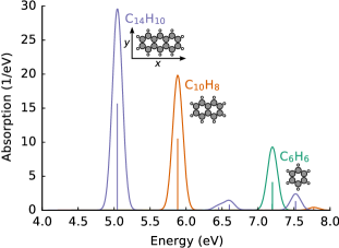
Figure 1: Photo-absorption spectra $S_{x}(\omega)$ along the long axis ($x$) of the benzene derivatives.

The response of each of the molecules is dominated by a single absorption peak (see Fig. 1), which results from discrete excitations. In Table 1, we show the KS decomposition of these excitations as described by the components of the normalized Casida eigenvectors $F_{I,ia}$. Due to the normalization, $\sum_{ia}F_{I,ia}^{2}=1$ for each excitation $I$.

For benzene (C6H6, point group $\text{D}_{6\text{h}}$) the excitation at 7.2 eV corresponds to the first $\text{E}_{\text{1u}}$ transition from the doubly degenerate highest occupied molecular orbital (HOMO; $\text{E}_{\text{1g}}$) to the doubly degenerate lowest unoccupied molecular orbital (LUMO; $\text{E}_{\text{2u}}$). In the present calculations the symmetry of the molecule has not been enforced and the orbitals $\pi_{-0/1}$ and $\pi^{*}_{+0/1}$ span the $\text{E}_{\text{1g}}$ and $\text{E}_{\text{2u}}$ symmetries, respectively. Implementation-dependent numerical factors slightly lift their degeneracy and determine the exact unitary rotation between the states.

Table 1: Casida analysis of the most prominent excitations of benzene (C6H6), naphthalene (C10H8), and naphthalene (C14H10). Orbitals are enumerated with respect to HOMO ($\pi_{-0}$) and LUMO ($\pi^{*}_{+0}$). The orbital characters are given in brackets based on the point groups $\text{D}_{\text{6h}}$ (benzene) and $\text{D}_{\text{2h}}$ (naphthalene, anthracene).

Molecule	$\omega_{I}$ (eV)	$f_{I}^{x}$	$i\,\to\,a$	$F^{2}_{I,ia}$
C6H6	$7.198$	$0.2784$	$\pi_{-1}(\text{E}_{\text{1g}})\,\to\,\pi^{*}_{+1}(\text{E}_{\text{2u}})$	0.31430
			$\pi_{-0}(\text{E}_{\text{1g}})\,\to\,\pi^{*}_{+0}(\text{E}_{\text{2u}})$	0.31254
			$\pi_{-1}(\text{E}_{\text{1g}})\,\to\,\pi^{*}_{+0}(\text{E}_{\text{2u}})$	0.16863
			$\pi_{-0}(\text{E}_{\text{1g}})\,\to\,\pi^{*}_{+1}(\text{E}_{\text{2u}})$	0.16833
	$7.199$	$1.3546$	$\pi_{-1}(\text{E}_{\text{1g}})\,\to\,\pi^{*}_{+0}(\text{E}_{\text{2u}})$	0.31362
			$\pi_{-0}(\text{E}_{\text{1g}})\,\to\,\pi^{*}_{+1}(\text{E}_{\text{2u}})$	0.31325
			$\pi_{-1}(\text{E}_{\text{1g}})\,\to\,\pi^{*}_{+1}(\text{E}_{\text{2u}})$	0.16895
			$\pi_{-0}(\text{E}_{\text{1g}})\,\to\,\pi^{*}_{+0}(\text{E}_{\text{2u}})$	0.16793
C10H8	$5.883$	$3.4839$	$\pi_{-0}(\text{A}_{\text{u}})\,\to\,\pi^{*}_{+1}(\text{B}_{\text{3g}})$	0.48451
			$\pi_{-1}(\text{B}_{\text{2u}})\,\to\,\pi^{*}_{+0}(\text{B}_{\text{1g}})$	0.47748
C14H10	$5.044$	$5.2000$	$\pi_{-0}(\text{B}_{\text{3g}})\,\to\,\pi^{*}_{+1}(\text{A}_{\text{u}})$	0.50237
			$\pi_{-1}(\text{B}_{\text{2g}})\,\to\,\pi^{*}_{+0}(\text{B}_{\text{1u}})$	0.45773
			$\pi_{-4}(\text{B}_{\text{1u}})\,\to\,\pi^{*}_{+2}(\text{B}_{\text{2g}})$	0.01049

Naphthalene (C10H8) and anthracene (C14H10) belong to the $\text{D}_{2\text{h}}$ symmetry point group. In both molecules the most prominent excitation is the $\text{B}_{\text{3u}}$ transition, which is mainly composed of transitions from HOMO to LUMO$+1$ and HOMO$-1$ to LUMO. While in naphthalene the other contributions amount to less than 1%, in anthracene, a minor contribution originates also from a transition from HOMO$-4$ to LUMO$+2$.

RT-TDDFT approach

The Casida eigenvector $F_{I,ia}$ considered in Table 1 is directly related to the linear response of the density matrix, see Eq. (13), and is employed here for benchmarking the RT-TDDFT methodology described Sec. II.1. In order to proceed with comparison, consider a discrete excitation $J$ that is energetically separated from other excitations. Since $\text{Im}[G_{I}(\omega_{J})]$ in Eq. (14) is approximately zero when $I\neq J$, only the excitation $J$ contributes in Eq. (13). This implies that $\text{Im}[\rho^{x}_{ia}(\omega_{J})]\approx A\sqrt{f_{ia}\omega_{ia}}F_{J,ia}$, where $A$ is a constant independent of index $ia$. Thus, after normalization, $\text{Im}[\rho^{x}_{ia}(\omega_{J})]/\sqrt{f_{ia}\omega_{ia}}\equiv F^{x}_{ia}(\omega_{J})$ yields the components of the Casida eigenvector $F_{J,ia}$. This connection allows us to calculate the Casida eigenvector also from the RT-TDDFT approach. This is demonstrated in Table 2, in which we show the calculated KS decompositions at the peak energies of the photo-absorption spectrum (Fig. 1).

Table 2: RT-TDDFT analysis at the peak energies $\omega$ of benzene (C6H6), naphthalene (C10H8), and naphthalene (C14H10). The intensities $S_{x}(\omega)$ have been multiplied with the area under the peak to facilitate a comparison with the oscillator strengths $f^{x}_{I}$ shown in Table 1. The last column shows for reference $[F^{x}_{ia}(\omega)]^{2}$ as calculated with the Casida approach.

Molecule	$\omega$ (eV)	$S_{x}(\omega)$	$i\,\to\,a$	$[F^{x}_{ia}(\omega)]^{2}$	Casida
C6H6	$7.20$	$1.6283$	$\pi_{-1}\,\to\,\pi^{*}_{+0}$	0.46184	0.46186
			$\pi_{-0}\,\to\,\pi^{*}_{+1}$	0.46126	0.46126
			$\pi_{-1}\,\to\,\pi^{*}_{+1}$	0.02045	0.02043
			$\pi_{-0}\,\to\,\pi^{*}_{+0}$	0.02032	0.02030
C10H8	$5.88$	$3.4776$	$\pi_{-0}\,\to\,\pi^{*}_{+1}$	0.48472	0.48451
			$\pi_{-1}\,\to\,\pi^{*}_{+0}$	0.47728	0.47748
C14H10	$5.04$	$5.1903$	$\pi_{-0}\,\to\,\pi^{*}_{+1}$	0.50277	0.50241
			$\pi_{-1}\,\to\,\pi^{*}_{+0}$	0.45745	0.45777
			$\pi_{-4}\,\to\,\pi^{*}_{+2}$	0.01044	0.01049

In the case of benzene (C6H6), we inevitably obtain a superposition of the two underlying degenerate excitations (see Table 1). We can, however, calculate the equivalent superimposed $F^{x}_{ia}(\omega)$ eigenvector also from the Casida approach (shown in the last column of Table 2). For this quantity, we obtain an excellent match between the RT-TDDFT and Casida approaches.

For naphthalene (C10H8) and anthracene (C14H10), a single excitation dominates the response and $F_{I,ia}^{2}$ and $[F^{x}_{ia}(\omega)]^{2}$ should yield the same decomposition as discussed above. Indeed, we observe that the RT-TDDFT calculations of the decomposition $[F^{x}_{ia}(\omega)]^{2}$ reproduce the discrete Casida eigenvector $F_{I,ia}^{2}$ with very good numerical accuracy. When both $F_{I,ia}^{2}$ and $[F^{x}_{ia}(\omega)]^{2}$ are calculated with the Casida approach, their values should be identical if the excitation is completely isolated. While for naphthalene, these quantities are exactly the same up to the shown number of digits (compare the last columns of Tables 1 and 2), for anthracene, the numerical values differ slightly. This deviation is due to a small contribution from a weak excitation that is close in energy ($\omega_{I}=5.051\,\text{eV}$, $f^{x}_{I}=5\cdot 10^{-4}$) to the dominant excitation of the anthracene molecule.

III.2 Silver nanoparticles

TDDFT calculations of noble metal nanoparticles up to diameters of several nanometers are computationally demanding, but the have become feasible with recent developments. Iida et al. (2014); Kuisma et al. (2015); Baseggio et al. (2015, 2016); Koval et al. (2016) Here, we focus on silver nanoparticles as prototypical nanoplasmonic systems with a strong plasmonic response in the visible–ultraviolet light regime. Scholl et al. (2012); Haberland (2013) Using the methodology described above in conjunction with a recent RT-TDDFT implementation Kuisma et al. (2015), we can analyze the response of silver nanoparticles with reasonable computational resources. For illustration, a full real-time propagation of 3000 time steps for Ag561 can be realized in 110 hours using 144 cores on an Intel Haswell based architecture. Not (a)

Kuisma et al. have previously studied icosahedral silver nanoparticles composed of 55, 147, 309, and 561 atoms corresponding to diameters ranging from $1.1$ nm to $2.7$ nm Kuisma et al. (2015). Here, we consider the same nanoparticle series and use the same geometries and computational parameters as in Ref. Kuisma et al., 2015. We employ optimized LCAO basis sets Kuisma et al. (2015) and the orbital-dependent Gritsenko-van Leeuwen-van Lenthe-Baerends (GLLB) Gritsenko et al. (1995) exchange-correlation potential with the solid-state modification by Kuisma et al. (GLLB-SC) Kuisma et al. (2010), which yields an accurate description of the $d$ electron states in noble metals. Yan et al. (2011, 2012); Kuisma et al. (2015)

The calculated photo-absorption spectra of the nanoparticles are shown in Fig. 2. The non-interacting-electron spectra calculated from the KS eigenvalue differences $\omega_{ia}$ and transition dipole matrix elements $\mu^{x}_{ia}$ are also shown to facilitate the discussion below. In Ref. Kuisma et al., 2015 it was observed that the plasmon resonance is well-formed in Ag147 and in larger nanoparticles, whereas the response of Ag55 consists of multiple peaks, the origin of which cannot be readily resolved. In the following, we analyze the response of nanoparticles in terms of the KS decomposition, which enables us to shed light on the response of the Ag55 nanoparticle.

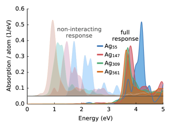
Figure 2: Photo-absorption spectra of icosahedral silver nanoparticles. The non-interacting-electron spectra shown for comparison are vertically shifted and scaled by a factor of $0.2$.

Transition contribution maps

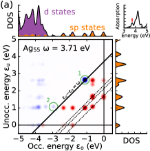
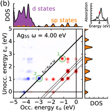
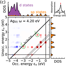
(a)

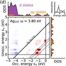
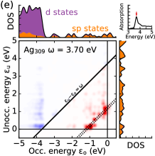
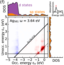
(b)

Figure 3: Transition contribution maps for the photo-absorption decomposition of Ag55 at different resonance energies $\omega$ (a–c), and those of Ag147 (d), Ag309 (e), and Ag561 (f) at the respective plasmon resonance energies. The KS eigenvalues are given with respect to the Fermi level. The constant transition energy lines $\varepsilon_{\text{u}}-\varepsilon_{\text{o}}=\omega$ are superimposed at the analysis energy (solid line) and at the resonance energies of the non-interacting-electron spectra (dashed lines, see Fig. 2). Red and blue colors indicate positive and negative values of the photo-absorption decomposition, respectively. The inset of each panel shows the absorption spectrum with the arrow pointing at the analysis frequency $\omega$. The densities of states (DOS) have been colored to indicate $sp$ and $d$ character of the states. The transitions marked with green circles in panels (a–c) are discussed in the text.

In order to analyze the response in terms of the Kohn–Sham decomposition, we present the decomposition as a transition contribution map (TCM; see Fig. 3 below) Malola et al. (2013); He and Zeng (2010), which is an especially useful representation for plasmonic systems in which resonances are typically superpositions of many electron-hole excitations. The TCM represents the KS decomposition weight $w_{ia}(\omega)$ at a fixed $\omega$ in the two-dimensional (2D) plane spanned by the energy axes for occupied and unoccupied states. More specifically, the 2D plot is defined by

$$M^{\text{TCM}}_{\omega}(\varepsilon_{\text{o}},\varepsilon_{\text{u}})=\sum_{ia}w_{ia}(\omega)g_{ia}(\varepsilon_{\text{o}},\varepsilon_{\text{u}}),$$ (18)

where $g_{ia}$ is a 2D broadening function of the discrete KS states. Here, we employ the Gaussian function

$$g_{ia}(\varepsilon_{\text{o}},\varepsilon_{\text{u}})=({\sqrt{2\pi}\sigma})^{-2}e^{{-\frac{(\varepsilon_{\text{o}}-\epsilon_{i})^{2}+(\varepsilon_{\text{u}}-\epsilon_{a})^{2}}{2\sigma^{2}}}}$$ (19)

with $\sigma=0.07\,\text{eV}$. The same $\sigma$ parameter is also used in the spectral broadening. For the weight $w_{ia}(\omega)$, we use the absorption decomposition of Eq. (17) normalized by the total absorption, i.e.,

$$w_{ia}(\omega)=S^{x}_{ia}(\omega)/S_{x}(\omega).$$ (20)

Due to the icosahedral symmetry of the nanoparticles their response is isotropic, $S_{x}(\omega)=S_{y}(\omega)=S_{z}(\omega)$, and the decomposition is degenerate (compare the case of benzene in Sec. III.1).

Alternatively, instead of Eq. (20) one could use, e.g., the normalized transition density matrix ($w_{ia}(\omega)=|\rho^{x}_{ia}(\omega)|^{2}$) as the weight. Equation (20), however, has the advantage that it retains the information about the sign of the response in the KS decomposition and has a physically sound interpretation as the photo-absorption decomposition.

TCMs of the nanoparticles at different resonance energies are shown in Fig. 3 along with the density of states (DOS), which has been colored to indicate the $sp$ and $d$ character of the states. The latter decomposition is based on the angular momentum quantum number $l_{\mu}$ of the LCAO basis functions indexed by $\mu$. For example, the $d$ character of the $n$th state is estimated as $\sum_{\mu:l_{\mu}=2}|C^{(0)}_{\mu n}|^{2}$, where the coefficients are normalized such that $\sum_{\mu}|C^{(0)}_{\mu n}|^{2}=1$.

Analysis of Ag₁₄₇, Ag₃₀₉, and Ag₅₆₁

First, we consider the largest nanoparticles Ag147, Ag309, and Ag561, the TCMs of which are shown in Figs. 3(d–f). The TCMs highlight two major features in their response. First, there is a strong positive constructive contribution Guidez and Aikens (2012) (red features in Fig. 3) from the KS transitions whose eigenvalue differences are significantly lower than the plasmon resonance energy $\omega$. The same low-energy $sp$ transitions are responsible for the strong peaks in the non-interacting-electron spectra (see Fig. 2), which are indicated in Fig. 3 by dashed lines. Thus, TCM shows how the resonance energy is blue-shifted as the interaction is turned on from the non-interacting case ($\lambda=0$) to the fully interacting one ($\lambda=1$). This demonstrates the plasmonic nature of the excitation in the so-called $\lambda$-scaling approach for plasmon identification, Bernadotte et al. (2013); Krauter et al. (2015) and illustrates the importance of low-energy transitions for plasmon formation. Ma et al. (2015) Another prominent feature in the response is the damping due to $d$ electrons, which is seen in the TCMs as large negative contributions from occupied $d$ states into unoccupied states (blue features at $\varepsilon_{\text{o}}\approx-4\,\text{eV}$ in Fig. 3). Interestingly, the plasmon peak appears close to the onset of $d$ electron transitions, corresponding to the intersection of the line $\varepsilon_{\text{u}}-\varepsilon_{\text{o}}=\omega$ and the horizontal Fermi level line. Generally, with increasing nanoparticle size the DOS becomes increasingly continuous, which is also visible in the increasing uniformity of the TCMs.

In Ref. Baseggio et al., 2016, TCMs for charged silver nanoparticles up to Ag309 have been studied. The two main features in Fig. 3, the low-energy $sp$ transitions and the $d$ electron damping, are in agreement with these TCMs reported earlier. In contrast to Fig. 3, the TCMs in Ref. Baseggio et al., 2016 show, however, also a significant contribution from $sp$ transitions close to the $\varepsilon_{\text{u}}-\varepsilon_{\text{o}}=\omega$ line. We consider this to be due to the different choice of the TCM weight $w_{ia}(\omega)$ in Ref. Baseggio et al., 2016. In the absorption decomposition we used in Fig. 3 [Eqs. (17) and (20)] the KS components are essentially weighted with the dipole matrix element $\mu^{x}_{ia}$, which affects the relative magnitudes observed in TCM.

Analysis of Ag₅₅

Next, we consider the Ag55 nanoparticle that exhibits multiple strong peaks in the absorption spectrum, resulting in difficulties in identifying the plasmon resonance. The TCM analyses for the three prominent peak energies are shown in Figs. 3(a–c). Due to its small size, Ag55 has well defined, discrete KS states as visible in DOS. The overall features in TCMs are similar to those of the larger nanoparticles, i.e., the low-energy $sp$ transitions and the $d$ electron transitions yield positive and negative contributions, respectively, though the low-energy transitions that form the plasmon are energetically clearly separated.

In contrast to the larger nanoparticles, in the Ag55 nanoparticle some of the strongly contributing $sp$ transitions are located close to the peak frequencies, i.e., close to the $\varepsilon_{\text{u}}-\varepsilon_{\text{o}}=\omega$ lines in the TCMs. These excitations are marked in Figs. 3(a–c) by green circles numbered as 1 and 2. By examining these KS transitions as a function of frequency $\omega$ (TCMs with the 0.01 eV resolution are provided as Supplemental Material Not (b)), we note that the first transition changes its sign at $\omega=3.85$ eV, close to the minimum between the peak maxima at 3.71 eV [Fig. 3(a)] and 4.00 eV (b). Similarly, the second transition changes its sign at $\omega=4.06$ eV between the maxima at 4.00 eV (b) and 4.20 eV (c). At the same time, the low-energy transitions forming the plasmon remain mainly unchanged over this frequency window. Thus, the presence of multiple peaks in the Ag55 spectrum seems to correspond to a strong coupling between the marked KS transitions and the plasmon. This is seen as the splitting of the plasmon into multiple resonances with antisymmetric and symmetric combinations of the KS transition and the plasmonic transitions. In the larger nanoparticles, the interaction between the plasmon and the nearby KS transitions is weak and the coupling is merely seen as a broadening of the plasmon peak.

A detailed inspection reveals that some $d$ electron transitions also change their sign in the frequency range where the peak splitting occurs. The changes in their sign, however, do not match the maxima and minima of the absorption spectrum like in the case of the marked KS transitions. Thus, we expect the marked $sp$ transitions to be the major cause for the plasmon splitting.

In the literature, Ag55 has been reported to have slightly varying spectra depending, e.g., on the exact geometry, the exchange-correlation functional, and the numerical parameters used. Weissker and Mottet (2011); Bae and Aikens (2012); Rabilloud (2014); Rossi et al. (2015b); Ma et al. (2015); Baseggio et al. (2016); Koval et al. (2016) Correspondingly, the electronic structures are different and the Ag55 spectra have single or multiple peaks. We expect, however, that the splitting behavior observed here can be a useful general concept for understanding the response of small plasmonic nanoparticles.

IV Discussion

The RT-TDDFT approach provides a more favorable scaling with the system size than the Casida approach. The latter, however, achieves a smaller pre-factor, especially when using non-local (e.g., hybrid exchange-correlation functionals) Sander and Kresse (2017), which renders it computationally more efficient for small and moderately-sized systems. In contrast, the RT-TDDFT approach becomes very attractive for systems comprising thousands of electrons (and typically hundreds of atoms) such as the silver nanoparticles considered in the present work. Previously, the lack of a decomposition scheme on par with the Casida method has been identified as a drawback of the RT-TDDFT approach. Sander and Kresse (2017) Here, we have introduced and demonstrated the performance of a method that overcomes this limitation and represents an efficient tool for analyzing electronic excitations within RT-TDDFT in general, and plasmonic response in particular.

It should be noted that in the RT-TDDFT approach the observable response is sensitive to the external perturbation used to initialize the time propagation. If the perturbation is chosen to be, say, a dipole perturbation along the $x$ direction, only excitations with a dipole component parallel to $x$ are observable in the response. By combining at most three separate time-propagation calculations (possibly even less in the cases of higher symmetry) with dipole perturbations along the $x$, $y$, and $z$ axes, one can recover the full dynamical polarizability tensor. However, for obtaining optically dark (dipole-forbidden) excitations from RT-TDDFT calculations, one would need to run the time propagation with different initial perturbations. This is in contrast to the Casida approach, where also dipole-forbidden excitations are obtained by diagonalizing the ${\bf\Omega}$ matrix.

It was illustrated in Sec. III.1 that the RT-TDDFT method does not yield direct access to the discrete spectrum, but rather allows an analysis at chosen frequencies yielding the combined response coming from all the contributing discrete excitations. Usually, this is not a significant restriction as in experimental measurements the energy resolution is limited by instrumental broadening and the excitation lifetimes. Computationally, the energy resolution is determined by the broadening parameter, which can be always reduced by increasing the propagation time. Furthermore, for larger systems that are the primary application area for RT-TDDFT, the electronic spectrum becomes increasingly dense and the distinction of individual excitations is less relevant.

V Conclusions

In this work we have presented that the linear response of the density matrix in the Kohn–Sham electron-hole basis can be obtained from real-time propagation TDDFT via a basis transformation. The methodology has been implemented in a recent RT-TDDFT code Kuisma et al. (2015) and is to be made publicly available as a part of the open source electronic structure code gpaw. Mortensen et al. (2005); Enkovaara et al. (2010); GPA

The present approach provides access to the same information via RT-TDDFT that is usually available only with the Casida approach. This was specifically demonstrated by a careful comparison of the results for benzene derivatives, which were shown to be numerically almost identical for the Casida and RT-TDDFT calculations.

Using the presented methodology, we analyzed the plasmonic response of icosahedral silver nanoparticles in the Kohn–Sham electron-hole space. The Ag55 nanoparticle was considered in detail and the multiple resonances in its response were shown to reflect the splitting of the plasmon due to the strong coupling between the plasmon and individual single-electron transitions. In the larger Ag147, Ag309, and Ag561 nanoparticles, the interaction between plasmon and individual single-electron transitions close to the resonance is weaker and a distinct plasmon resonance emerges from the constructive superposition of the low-energy Kohn–Sham transitions Bernadotte et al. (2013); Krauter et al. (2015); Ma et al. (2015) accompanied by the damping due to $d$ electron transitions.

In summary, the present work raises the analysis capabilities of the RT-TDDFT to the same level as with the Casida approach, without compromising the computational benefits of RT-TDDFT.

*

Appendix A Derivation of Eq. (9) within the PAW formalism

Within the PAW formalism, Eq. (1) reads

$$i\mathcal{T}^{\dagger}\mathcal{T}\frac{\partial}{\partial t}\widetilde{\psi}_{n}(\boldsymbol{r},t)=\mathcal{T}^{\dagger}H_{\text{KS}}(t)\mathcal{T}\widetilde{\psi}_{n}(\boldsymbol{r},t),$$ (21)

where $\widetilde{\psi}_{n}(\boldsymbol{r},t)$ is a pseudo wave function and $\mathcal{T}$ denotes the PAW transformation operator Blöchl (1994).

In the LCAO method, the pseudo wave function $\widetilde{\psi}_{n}(\boldsymbol{r},t)$ is expanded in localized basis functions $\widetilde{\phi}_{\mu}(\boldsymbol{r})$ centered at atomic coordinates

$$\widetilde{\psi}_{n}(\boldsymbol{r},t)=\sum_{\mu}\widetilde{\phi}_{\mu}(\boldsymbol{r})C_{\mu n}(t),$$ (22)

with expansion coefficients $C_{\mu n}(t)$. The corresponding all-electron wave function is given by [compare to Eq. (7)]

$$\psi_{n}(\boldsymbol{r},t)=\mathcal{T}\widetilde{\psi}_{n}(\boldsymbol{r},t)=\sum_{\mu}\phi_{\mu}(\boldsymbol{r})C_{\mu n}(t),$$ (23)

where the all-electron basis functions have been defined as $\phi_{\mu}=\mathcal{T}\widetilde{\phi}_{\mu}$.

The time-dependent all-electron real-space density matrix can be obtained as

$$\rho(\boldsymbol{r},\boldsymbol{r}^{\prime},t)=\sum_{\mu\nu}\phi_{\mu}(\boldsymbol{r})\rho_{\mu\nu}(t)\phi_{\nu}^{*}(\boldsymbol{r}^{\prime}),$$ (24)

where the density matrix in the LCAO basis $\rho_{\mu\nu}(t)$ is given by Eq. (8).

The transformation of the real-space density matrix to the basis defined by the ground-state KS orbitals $\psi_{n}^{(0)}(\boldsymbol{r})$, see Eq. (3), is given by

$$\rho_{nn^{\prime}}(t)=\int{\rm d}\boldsymbol{r}\int{\rm d}\boldsymbol{r}^{\prime}\psi_{n}^{(0)*}(\boldsymbol{r})\rho(\boldsymbol{r},\boldsymbol{r}^{\prime},t)\psi_{n^{\prime}}^{(0)}(\boldsymbol{r}^{\prime}).$$ (25)

By expanding $\psi_{n}^{(0)}(\boldsymbol{r})$ in the LCAO basis as in Eq. (23) and inserting Eq. (24) into Eq. (25), we obtain after reordering the integrals

$$\rho_{nn^{\prime}}(t) =\sum_{\mu}C^{(0)*}_{\mu n}\sum_{\mu^{\prime}}\underbrace{\int\text{d}\boldsymbol{r}\phi_{\mu}^{*}(\boldsymbol{r})\phi_{\mu^{\prime}}(\boldsymbol{r})}_{S_{\mu\mu^{\prime}}}$$

$$\cdot\sum_{\nu^{\prime}}\rho_{\mu^{\prime}\nu^{\prime}}(t)\sum_{\nu}\underbrace{\int\text{d}\boldsymbol{r}^{\prime}\phi_{\nu^{\prime}}^{*}(\boldsymbol{r}^{\prime})\phi_{\nu}(\boldsymbol{r}^{\prime})}_{S^{*}_{\nu\nu^{\prime}}}C^{(0)}_{\nu n^{\prime}}.$$ (26)

Here, we have isolated the overlap integrals $S_{\mu\mu^{\prime}}$ used regularly in LCAO calculations, i.e.,

$$S_{\mu\mu^{\prime}}=\int\text{d}\boldsymbol{r}\phi^{*}_{\mu}(\boldsymbol{r})\phi_{\mu^{\prime}}(\boldsymbol{r})=\int\text{d}\boldsymbol{r}\widetilde{\phi}^{*}_{\mu}(\boldsymbol{r})\mathcal{T}^{\dagger}\mathcal{T}\widetilde{\phi}_{\mu^{\prime}}(\boldsymbol{r}).$$ (27)

After simplifying the overlap integrals in Eq. (26), we obtain Eq. (9). We note that the PAW transformation affects only the evaluation of the overlap integrals $S_{\mu\mu^{\prime}}$, see Eq. (27).

References

- Runge and Gross (1984) E. Runge and E. K. U. Gross, Phys. Rev. Lett. 52, 997 (1984).
- Hohenberg and Kohn (1964) P. Hohenberg and W. Kohn, Phys. Rev. 136, B864 (1964).
- Kohn and Sham (1965) W. Kohn and L. J. Sham, Phys. Rev. 140, A1133 (1965).
- Marques et al. (2012) M. A. L. Marques, N. T. Maitra, F. M. S. Nogueira, E. K. U. Gross, and A. Rubio, eds., Fundamentals of Time-Dependent Density Functional Theory, Lecture Notes in Physics, Vol. 837 (Springer, 2012).
- Ullrich (2012) C. A. Ullrich, Time-Dependent Density-Functional Theory: Concepts and Applications (Oxford University Press, 2012).
- Ekardt (1984) W. Ekardt, Phys. Rev. Lett. 52, 1925 (1984).
- Puska et al. (1985) M. J. Puska, R. M. Nieminen, and M. Manninen, Phys. Rev. B 31, 3486 (1985).
- Beck (1987) D. E. Beck, Phys. Rev. B 35, 7325 (1987).
- Morton et al. (2011) S. M. Morton, D. W. Silverstein, and L. Jensen, Chem. Rev. 111, 3962 (2011).
- Varas et al. (2016) A. Varas, P. García-González, J. Feist, F. García-Vidal, and A. Rubio, Nanophotonics 5, 409 (2016).
- Prodan et al. (2003) E. Prodan, P. Nordlander, and N. J. Halas, Nano Lett. 3, 1411 (2003).
- Aikens et al. (2008) C. M. Aikens, S. Li, and G. C. Schatz, J. Phys. Chem. C 112, 11272 (2008).
- Zuloaga et al. (2010) J. Zuloaga, E. Prodan, and P. Nordlander, ACS Nano 4, 5269 (2010).
- Weissker and Mottet (2011) H.-C. Weissker and C. Mottet, Phys. Rev. B 84, 165443 (2011).
- Li et al. (2013) J.-H. Li, M. Hayashi, and G.-Y. Guo, Phys. Rev. B 88, 155437 (2013).
- Piccini et al. (2013) G. Piccini, R. W. A. Havenith, R. Broer, and M. Stener, J. Phys. Chem. C 117, 17196 (2013).
- Burgess and Keast (2014) R. W. Burgess and V. J. Keast, J. Phys. Chem. C 118, 3194 (2014).
- Barcaro et al. (2014) G. Barcaro, L. Sementa, A. Fortunelli, and M. Stener, J. Phys. Chem. C 118, 12450 (2014).
- Weissker and Lopez-Lozano (2015) H.-C. Weissker and X. Lopez-Lozano, Phys. Chem. Chem. Phys. 17, 28379 (2015).
- Bae and Aikens (2015) G.-T. Bae and C. M. Aikens, J. Phys. Chem. C 119, 23127 (2015).
- Zapata Herrera et al. (2016) M. Zapata Herrera, J. Aizpurua, A. K. Kazansky, and A. G. Borisov, Langmuir 32, 2829 (2016).
- Zuloaga et al. (2009) J. Zuloaga, E. Prodan, and P. Nordlander, Nano Lett. 9, 887 (2009).
- Song et al. (2011) P. Song, P. Nordlander, and S. Gao, J. Chem. Phys. 134, 074701 (2011).
- Song et al. (2012) P. Song, S. Meng, P. Nordlander, and S. Gao, Phys. Rev. B 86, 121410 (2012).
- Marinica et al. (2012) D. Marinica, A. Kazansky, P. Nordlander, J. Aizpurua, and A. G. Borisov, Nano Lett. 12, 1333 (2012).
- Zhang et al. (2014) P. Zhang, J. Feist, A. Rubio, P. García-González, and F. J. García-Vidal, Phys. Rev. B 90, 161407 (2014).
- Varas et al. (2015) A. Varas, P. García-González, F. J. García-Vidal, and A. Rubio, J. Phys. Chem. Lett. 6, 1891 (2015).
- Barbry et al. (2015) M. Barbry, P. Koval, F. Marchesin, R. Esteban, A. G. Borisov, J. Aizpurua, and D. Sánchez-Portal, Nano Lett. 15, 3410 (2015).
- Kulkarni and Manjavacas (2015) V. Kulkarni and A. Manjavacas, ACS Photonics 2, 987 (2015).
- Rossi et al. (2015a) T. P. Rossi, A. Zugarramurdi, M. J. Puska, and R. M. Nieminen, Phys. Rev. Lett. 115, 236804 (2015a).
- Marchesin et al. (2016) F. Marchesin, P. Koval, M. Barbry, J. Aizpurua, and D. Sánchez-Portal, ACS Photonics 3, 269 (2016).
- Lahtinen et al. (2016) T. Lahtinen, E. Hulkko, K. Sokolowska, T.-R. Tero, V. Saarnio, J. Lindgren, M. Pettersson, H. Hakkinen, and L. Lehtovaara, Nanoscale 8, 18665 (2016).
- Manjavacas et al. (2013) A. Manjavacas, F. Marchesin, S. Thongrattanasiri, P. Koval, P. Nordlander, D. Sánchez-Portal, and F. J. García de Abajo, ACS Nano 7, 3635 (2013).
- Andersen and Thygesen (2013) K. Andersen and K. S. Thygesen, Phys. Rev. B 88, 155128 (2013).
- Andersen et al. (2014) K. Andersen, K. W. Jacobsen, and K. S. Thygesen, Phys. Rev. B 90, 161410 (2014).
- Lauchner et al. (2015) A. Lauchner, A. E. Schlather, A. Manjavacas, Y. Cui, M. J. McClain, G. J. Stec, F. J. García de Abajo, P. Nordlander, and N. J. Halas, Nano Lett. 15, 6208 (2015).
- Gao and Yuan (2005) S. Gao and Z. Yuan, Phys. Rev. B 72, 121406 (2005).
- Yan et al. (2007) J. Yan, Z. Yuan, and S. Gao, Phys. Rev. Lett. 98, 216602 (2007).
- Bernadotte et al. (2013) S. Bernadotte, F. Evers, and C. R. Jacob, J. Phys. Chem. C 117, 1863 (2013).
- Malola et al. (2013) S. Malola, L. Lehtovaara, J. Enkovaara, and H. Häkkinen, ACS Nano 7, 10263 (2013).
- Guidez and Aikens (2012) E. B. Guidez and C. M. Aikens, Nanoscale 4, 4190 (2012).
- Guidez and Aikens (2014) E. B. Guidez and C. M. Aikens, Nanoscale 6, 11512 (2014).
- Yasuike et al. (2011) T. Yasuike, K. Nobusada, and M. Hayashi, Phys. Rev. A 83, 013201 (2011).
- Casanova et al. (2016) D. Casanova, J. M. Matxain, and J. M. Ugalde, J. Phys. Chem. C 120, 12742 (2016).
- Townsend and Bryant (2012) E. Townsend and G. W. Bryant, Nano Lett. 12, 429 (2012).
- Townsend and Bryant (2014) E. Townsend and G. W. Bryant, J. Opt. 16, 114022 (2014).
- Ma et al. (2015) J. Ma, Z. Wang, and L.-W. Wang, Nat. Commun. 6, 10107 (2015).
- Bursi et al. (2016) L. Bursi, A. Calzolari, S. Corni, and E. Molinari, ACS Photonics 3, 520 (2016).
- Esteban et al. (2012) R. Esteban, A. G. Borisov, P. Nordlander, and J. Aizpurua, Nat. Commun. 3, 825 (2012).
- Stella et al. (2013) L. Stella, P. Zhang, F. J. García-Vidal, A. Rubio, and P. García-González, J. Phys. Chem. C 117, 8941 (2013).
- Chen et al. (2015) X. Chen, J. E. Moore, M. Zekarias, and L. Jensen, Nat. Commun. 6, 8921 (2015).
- Yan et al. (2015) W. Yan, M. Wubs, and N. Asger Mortensen, Phys. Rev. Lett. 115, 137403 (2015).
- Teperik et al. (2016) T. V. Teperik, A. K. Kazansky, and A. G. Borisov, Phys. Rev. B 93, 155431 (2016).
- Ciracì and Della Sala (2016) C. Ciracì and F. Della Sala, Phys. Rev. B 93, 205405 (2016).
- David et al. (2016) C. David, J. Christensen, and N. A. Mortensen, Phys. Rev. B 94, 165410 (2016).
- (56) T. Christensen, W. Yan, A.-P. Jauho, M. Soljacic, and N. A. Mortensen, Phys. Rev. Lett., in press (2017). arXiv:1608.05421v2.
- Ciracì et al. (2012) C. Ciracì, R. T. Hill, J. J. Mock, Y. Urzhumov, A. I. Fernández-Domínguez, S. A. Maier, J. B. Pendry, A. Chilkoti, and D. R. Smith, Science 337, 1072 (2012).
- Scholl et al. (2012) J. A. Scholl, A. L. Koh, and J. A. Dionne, Nature 483, 421 (2012).
- Haberland (2013) H. Haberland, Nature 494, E1 (2013).
- Savage et al. (2012) K. J. Savage, M. M. Hawkeye, R. Esteban, A. G. Borisov, J. Aizpurua, and J. J. Baumberg, Nature 491, 574 (2012).
- Banik et al. (2012) M. Banik, P. Z. El-Khoury, A. Nag, A. Rodriguez-Perez, N. Guarrottxena, G. C. Bazan, and V. A. Apkarian, ACS Nano 6, 10343 (2012).
- Banik et al. (2013) M. Banik, V. A. Apkarian, T.-H. Park, and M. Galperin, J. Phys. Chem. Lett. 4, 88 (2013).
- Scholl et al. (2013) J. A. Scholl, A. García-Etxarri, A. L. Koh, and J. A. Dionne, Nano Lett. 13, 564 (2013).
- Tan et al. (2014) S. F. Tan, L. Wu, J. K. Yang, P. Bai, M. Bosman, and C. A. Nijhuis, Science 343, 1496 (2014).
- Zhang et al. (2016) C. Zhang, H. Zhao, L. Zhou, A. E. Schlather, L. Dong, M. J. McClain, D. F. Swearer, P. Nordlander, and N. J. Halas, Nano Lett. 16, 6677 (2016).
- Sanders et al. (2016) A. Sanders, R. W. Bowman, and J. J. Baumberg, Sci. Rep. 6, 32988 (2016).
- Mertens et al. (2016) J. Mertens, A. Demetriadou, R. W. Bowman, F. Benz, M.-E. Kleemann, C. Tserkezis, Y. Shi, H. Y. Yang, O. Hess, J. Aizpurua, and J. J. Baumberg, Nano Lett. 16, 5605 (2016).
- Tame et al. (2013) M. S. Tame, K. R. McEnery, S. K. Ozdemir, J. Lee, S. A. Maier, and M. S. Kim, Nat. Phys. 9, 329 (2013).
- Zhu et al. (2016) W. Zhu, R. Esteban, A. G. Borisov, J. J. Baumberg, P. Nordlander, H. J. Lezec, J. Aizpurua, and K. B. Crozier, Nat. Commun. 7, 11495 (2016).
- Iida et al. (2014) K. Iida, M. Noda, K. Ishimura, and K. Nobusada, J. Phys. Chem. A 118, 11317 (2014).
- Kuisma et al. (2015) M. Kuisma, A. Sakko, T. P. Rossi, A. H. Larsen, J. Enkovaara, L. Lehtovaara, and T. T. Rantala, Phys. Rev. B 91, 115431 (2015).
- Baseggio et al. (2015) O. Baseggio, G. Fronzoni, and M. Stener, J. Chem. Phys. 143, 024106 (2015).
- Baseggio et al. (2016) O. Baseggio, M. De Vetta, G. Fronzoni, M. Stener, L. Sementa, A. Fortunelli, and A. Calzolari, J. Phys. Chem. C 120, 12773 (2016).
- Koval et al. (2016) P. Koval, F. Marchesin, D. Foerster, and D. Sánchez-Portal, J. Phys.: Condens. Matter 28, 214001 (2016).
- Casida (1995) M. E. Casida, in Recent Advances in Density Functional Methods, Part I, edited by D. P. Chong (World Scientific, Singapore, 1995) p. 155.
- Petersilka et al. (1996) M. Petersilka, U. J. Gossmann, and E. K. U. Gross, Phys. Rev. Lett. 76, 1212 (1996).
- Casida (2009) M. E. Casida, J. Mol. Struct. THEOCHEM 914, 3 (2009).
- Bauernschmitt and Ahlrichs (1996) R. Bauernschmitt and R. Ahlrichs, Chem. Phys. Lett. 256, 454 (1996).
- Stratmann et al. (1998) R. E. Stratmann, G. E. Scuseria, and M. J. Frisch, J. Chem. Phys. 109, 8218 (1998).
- Walker et al. (2006) B. Walker, A. M. Saitta, R. Gebauer, and S. Baroni, Phys. Rev. Lett. 96, 113001 (2006).
- Andrade et al. (2007) X. Andrade, S. Botti, M. A. L. Marques, and A. Rubio, J. Chem. Phys. 126, 184106 (2007).
- Yabana and Bertsch (1996) K. Yabana and G. F. Bertsch, Phys. Rev. B 54, 4484 (1996).
- Yabana et al. (2006) K. Yabana, T. Nakatsukasa, J.-I. Iwata, and G. F. Bertsch, Phys. Status Solidi B 243, 1121 (2006).
- Sander and Kresse (2017) T. Sander and G. Kresse, J. Chem. Phys. 146, 064110 (2017).
- Yan et al. (2016) L. Yan, F. Wang, and S. Meng, ACS Nano 10, 5452 (2016).
- Li and Ullrich (2011) Y. Li and C. A. Ullrich, Chem. Phys. 391, 157 (2011).
- Li and Ullrich (2015) Y. Li and C. A. Ullrich, J. Chem. Theory Comput. 11, 5838 (2015).
- Repisky et al. (2015) M. Repisky, L. Konecny, M. Kadek, S. Komorovsky, O. L. Malkin, V. G. Malkin, and K. Ruud, J. Chem. Theory Comput. 11, 980 (2015).
- Kolesov et al. (2016) G. Kolesov, O. Grånäs, R. Hoyt, D. Vinichenko, and E. Kaxiras, J. Chem. Theory Comput. 12, 466 (2016).
- Malola et al. (2014) S. Malola, L. Lehtovaara, and H. Häkkinen, J. Phys. Chem. C 118, 20002 (2014).
- Malola et al. (2015) S. Malola, M. J. Hartmann, and H. Häkkinen, J. Phys. Chem. Lett. 6, 515 (2015).
- Larsen et al. (2009) A. H. Larsen, M. Vanin, J. J. Mortensen, K. S. Thygesen, and K. W. Jacobsen, Phys. Rev. B 80, 195112 (2009).
- Mortensen et al. (2005) J. J. Mortensen, L. B. Hansen, and K. W. Jacobsen, Phys. Rev. B 71, 035109 (2005).
- Enkovaara et al. (2010) J. Enkovaara, C. Rostgaard, J. J. Mortensen, J. Chen, M. Dułak, L. Ferrighi, J. Gavnholt, C. Glinsvad, V. Haikola, H. A. Hansen, H. H. Kristoffersen, M. Kuisma, A. H. Larsen, L. Lehtovaara, M. Ljungberg, O. Lopez-Acevedo, P. G. Moses, J. Ojanen, T. Olsen, V. Petzold, N. A. Romero, J. Stausholm-Møller, M. Strange, G. A. Tritsaris, M. Vanin, M. Walter, B. Hammer, H. Häkkinen, G. K. H. Madsen, R. M. Nieminen, J. K. Nørskov, M. Puska, T. T. Rantala, J. Schiøtz, K. S. Thygesen, and K. W. Jacobsen, J. Phys.: Condens. Matter 22, 253202 (2010).
- (95) “GPAW: DFT and beyond within the projector-augmented wave method,” https://wiki.fysik.dtu.dk/gpaw/.
- Blöchl (1994) P. E. Blöchl, Phys. Rev. B 50, 17953 (1994).
- Walter et al. (2008) M. Walter, H. Häkkinen, L. Lehtovaara, M. Puska, J. Enkovaara, C. Rostgaard, and J. J. Mortensen, J. Chem. Phys. 128, 244101 (2008).
- Wilkinson (1956) P. G. Wilkinson, Can. J. Phys. 34, 596 (1956).
- Ferguson et al. (1957) J. Ferguson, L. W. Reeves, and W. G. Schneider, Can. J. Chem. 35, 1117 (1957).
- Rossi et al. (2015b) T. P. Rossi, S. Lehtola, A. Sakko, M. J. Puska, and R. M. Nieminen, J. Chem. Phys. 142, 094114 (2015b).
- Perdew et al. (1996) J. P. Perdew, K. Burke, and M. Ernzerhof, Phys. Rev. Lett. 77, 3865 (1996).
- Perdew et al. (1997) J. P. Perdew, K. Burke, and M. Ernzerhof, Phys. Rev. Lett. 78, 1396 (1997).
- Not (a) The timing was performed on the Taito supercluster of CSC – IT Center for Science, Finland. Each computing node has Intel Haswell E5-2690v3 processors and the nodes are connected with Infiniband FDR interconnect. For further details of the hardware, see https://research.csc.fi/taito-supercluster (9th Feb 2017).
- Gritsenko et al. (1995) O. Gritsenko, R. van Leeuwen, E. van Lenthe, and E. J. Baerends, Phys. Rev. A 51, 1944 (1995).
- Kuisma et al. (2010) M. Kuisma, J. Ojanen, J. Enkovaara, and T. T. Rantala, Phys. Rev. B 82, 115106 (2010).
- Yan et al. (2011) J. Yan, K. W. Jacobsen, and K. S. Thygesen, Phys. Rev. B 84, 235430 (2011).
- Yan et al. (2012) J. Yan, K. W. Jacobsen, and K. S. Thygesen, Phys. Rev. B 86, 241404 (2012).
- He and Zeng (2010) Y. He and T. Zeng, J. Phys. Chem. C 114, 18023 (2010).
- Krauter et al. (2015) C. M. Krauter, S. Bernadotte, C. R. Jacob, M. Pernpointner, and A. Dreuw, J. Phys. Chem. C 119, 24564 (2015).
- Not (b) See Supplemental Material for additional transition contribution maps for the Ag55 nanoparticle.
- Bae and Aikens (2012) G.-T. Bae and C. M. Aikens, J. Phys. Chem. C 116, 10356 (2012).
- Rabilloud (2014) F. Rabilloud, J. Chem. Phys. 141, 144302 (2014).