Discretized Keiper/Li approach
to the Riemann Hypothesis

Abstract

The Keiper–Li sequence $\{\lambda_{n}\}$ is most sensitive to the Riemann Hypothesis asymptotically ($n\to\infty$), but highly elusive both analytically and numerically. We deform it to fully explicit sequences, simpler to analyze and to compute (up to $n=5\cdot 10^{5}$ by G. Misguich). This also works on the Davenport–Heilbronn counterexamples, thus we can demonstrate explicit tests that selectively react to zeros off the critical line.

The present text develops our computations announced from 2015 [36] on a novel type of explicit sequential criteria for the Riemann Hypothesis.

The Riemann zeta function $\zeta(x):$ e.g., [32][11, chaps. 8, 15], has countably many zeros $\rho$ in the upper half-plane $\{\mathop{\rm Im\,}\nolimits\rho>0\}$, which accumulate to $+{\rm i}\infty$ (and their complex-conjugates, which we will not count). The Riemann Hypothesis (RH) [27] states that all those zeros lie on the critical line ${\{\mathop{\rm Re\,}\nolimits\rho={\textstyle{1\over 2}}\}}$, and this remains a major open conjecture.

Within bounded heights $T=\mathop{\rm Im\,}\nolimits\rho$ on the other hand, direct tests have always validated $\mathop{\rm Re\,}\nolimits\rho\equiv{\textstyle{1\over 2}}$, now up to the $10^{13}$-th zero [16]. If $T_{0}$ denotes the highest $T$ up to which RH is verified (at a given time), that roughly sets

$$T_{0}\approx 2.4\cdot 10^{12}\quad\mbox{currently (as of 2004)}.$$ (1)

We will examine how novel sequential criteria might probe RH further, i.e., sense any zeros $\rho^{\prime}={\textstyle{1\over 2}}+t+{\rm i}T$ with $t>0$ (violating RH) and $T>T_{0}$.

First (§ 1) we review the usual Keiper–Li constants $\{\lambda_{n}\}_{n\geq 1}$. Their (real-valued) sequence is RH-sensitive and could detect such $\rho^{\prime}$ for ${n\gtrsim T^{2}/t}$ (currently: above $\approx 10^{25}$). But the $\lambda_{n}$ involve derivatives of $\log\zeta$ to any orders, which are most elusive both analytically and numerically (in which case the difficulty steeply rises with $n:$ only recently was $n=10^{5}$ reached).

We propose instead (§ 2) to modify the Keiper–Li definition, by discretizing the above derivatives to finite differences while retaining RH-sensitivity. We thus obtain a variant sequence $\{\Lambda_{n}\}$ in the elementary explicit form (36), also more expedient to encode numerically (G. Misguich reached $n=5\cdot 10^{5}$).

In § 3 we confirm analytically that the sequence $\{\Lambda_{n}\}$ is RH-sensitive, in its asymptotic tail like $\{\lambda_{n}\}$, just a bit less simply; we also extend the framework to certain Dirichlet L-series.

In § 4 we initiate quantitative and numerical studies. We find two main thresholds for the visibility of the above $\rho^{\prime}$ through $\{\Lambda_{n}\}:$ for $n\gtrsim T^{1+2/t}$ (currently: above $\approx 10^{60}$) detection is certain; inversely for $n\lesssim{\textstyle{1\over 2}}T\mathop{\rm e}\nolimits^{1/t}$ (currently $\approx 10^{13}$ or higher) detection is outright barred by an uncertainty principle. Somewhere in-between, achievable sensitivity will depend on how deeply $\{\Lambda_{n}\}$ can be described and processed in the future. In any case and like $\{\lambda_{n}\}$, $\{\Lambda_{n}\}$ probes RH in a complementary manner to the classic direct methods (Riemann–Siegel based), currently more efficient but strictly local in $T$. Thanks to the Davenport–Heilbronn counterexamples, we can concretely demonstrate how a (generalized) $\Lambda_{n}$-sequence signals $\mathop{\rm Re\,}\nolimits\rho^{\prime}\neq{\textstyle{1\over 2}}$.

We finally analyze in detail the loss of precision in the numerical calculation of $\Lambda_{n}$. It grows linearly with $n$, being on average twice that for $\lambda_{n}$, but for $\Lambda_{n}$ that is the sole computational stumbling block, and a purely logistic one (arbitrary-precision programs are fully ready, only computing power has to rise to the task). Hence overall, $\{\Lambda_{n}\}$ is easier to calculate, has a lower uncertainty-principle barrier, and its study only begins. This discretized version of the Keiper–Li sequence thus ought to be more efficient in the long run than the original $\{\lambda_{n}\}$ for testing RH further.

An Appendix describes a similar discretization for a variant (more symmetrical) Keiper–Li sequence.

1 Main notations and background

$\bullet\ 2\xi(\cdot):$ a completed zeta function, obeying Riemann’s Functional Equation,

$$2\xi(x)\stackrel{{\scriptstyle\rm def}}{{=}}x(x-1)\pi^{-x/2}\,\Gamma(x/2)\,\zeta(x)\equiv 2\xi(1-x):$$ (2)

$2\xi$ is better normalized for us than Riemann’s $\xi$-function: $2\xi(0)=2\xi(1)=1$.

The symmetry in (2) makes us also denote $x={\textstyle{1\over 2}}+t+{\rm i}T\$ ($t,T$ real).

$\bullet\ \{\rho\}:$ the set of zeros of $\xi$ (the nontrivial zeros of $\zeta$ or Riemann zeros, counted with multiplicities if any); this set has the symmetry axes $\mathbb{R}$ and ${L\stackrel{{\scriptstyle\rm def}}{{=}}\{\mathop{\rm Re\,}\nolimits x={\textstyle{1\over 2}}\}}$ (the critical line), it lies in the critical strip ${\{0<\mathop{\rm Re\,}\nolimits x<1\}}$, and its ordinate-counting function $N(T)\stackrel{{\scriptstyle\rm def}}{{=}}\#\{\rho\mid 0\leq\mathop{\rm Im\,}\nolimits\rho\leq T\}$ has the Riemann–von Mangoldt asymptotic form:

$$N(T)=\overline{N}(T)+O(\log T)\quad\mbox{for }T\to+\infty,\quad\mbox{with }\overline{N}(T)=\frac{T}{2\pi}\log\frac{T}{2\pi{\rm e}}\,;$$ (3)

infinite summations over zeros are meant to be ordered symmetrically, as

$$\sum_{\rho}\stackrel{{\scriptstyle\rm def}}{{=}}\lim_{T\to\infty}\sum_{|\mathop{\rm Im\,}\nolimits\rho|\leq T}.$$ (4)

We will dub $\rho^{\prime}$ any zeros for which we assume $\mathop{\rm Re\,}\nolimits\rho^{\prime}>{\textstyle{1\over 2}}$ (violating RH).

$\bullet\ \zeta(x,w)\stackrel{{\scriptstyle\rm def}}{{=}}\sum\limits_{k=0}^{\infty}(k+w)^{-x}:$ the Hurwitz zeta function.

$\bullet\ \Gamma(\cdot):$ the Euler Gamma function,  $\gamma:$ Euler’s constant ($\approx 0.5772156649$).

$\bullet\ k!!:$ the double factorial, used here for odd integers $k$ only, in which case

$$k!!\!\!\! \stackrel{{\scriptstyle\rm def}}{{=}} \!\!\!k(k-2)\cdots 1\qquad\qquad\quad\mbox{for odd }k>0,$$

$$\stackrel{{\scriptstyle\rm def}}{{=}} \!\!\!2^{(k+1)/2}\,\Gamma({\textstyle{1\over 2}}k+1)/\sqrt{\pi}\quad\mbox{for odd }k\gtrless 0\quad(e.g.,\ (-1)!!=1,\ (-3)!!=-1).$$

$\bullet\ (j,k,\ell)!\stackrel{{\scriptstyle\rm def}}{{=}}(j+k+\ell)!\,/\,(j!\,k!\,\ell!)$  (3-index multinomial coefficients).

$\bullet\ B_{2m}:$ Bernoulli numbers, $B_{2m}(\cdot):$ Bernoulli polynomials  ($m=0,1,2,\ldots$).

1.1 The Keiper and Li coefficients

In 1992 Keiper [19] considered a real sequence $\{\lambda_{n}\}$ of generating function

$$\varphi(z)\stackrel{{\scriptstyle\rm def}}{{=}}\log 2\xi(M(z))\equiv\sum_{n=1}^{\infty}\lambda^{\rm K}_{n}\,z^{n},\qquad M(z)\stackrel{{\scriptstyle\rm def}}{{=}}\frac{1}{1-z},$$ (5)

(we write $\lambda^{\rm K}_{n}$ for Keiper’s $\lambda_{n}$), deduced that

$$\lambda^{\rm K}_{n}\equiv n^{-1}\sum_{\rho}\bigl{[}1-(1-1/\rho)^{n}\bigr{]},$$ (6)

and that RH $\Rightarrow\ \lambda^{\rm K}_{n}>0\ (\forall n)$, then wrote (without proof nor elaboration): “In fact, if we assume the Riemann hypothesis, and further that the zeros are very evenly distributed, we can show that

$$\lambda_{m}\approx\frac{\log m}{2}-\frac{\log(2\pi)+1-\gamma}{2}.\,{"\atop}\quad\mbox{[for $\lambda^{\rm K}_{m}\,$; \ $m\to\infty$ seems implied.}]$$ (7)

In (5), the conformal mapping $M:z\mapsto x$ acts to pull back each zero $\rho$ to

$$z_{\rho}\stackrel{{\scriptstyle\rm def}}{{=}}M^{-1}(\rho)=1-1/\rho,$$ (8)

and the critical line $L$ to the unit circle $\{|z|=1\}$, ensuring that (Fig. 1):

$$\mbox{RH}\iff|z_{\rho}|\equiv 1\ (\forall\rho)\iff\varphi\mbox{ is \emph{regular in the whole disk} }\{|z|<1\}.$$ (9)

In 1997 Li [21] independently introduced another sequence $\{\lambda_{n}\}$, through

$$\lambda^{\rm L}_{n}=\frac{1}{(n-1)!}\,\frac{{\rm d}^{n}}{{\rm d}x^{n}}\bigl{[}x^{n-1}\log 2\xi(x)\bigr{]}_{x=1},\quad n=1,2,\ldots,$$ (10)

(we write $\lambda^{\rm L}_{n}$ for Li’s $\lambda_{n}$), and proved the sharp equivalence (Li’s criterion):

$$\mbox{RH}\quad\iff\quad\lambda^{\rm L}_{n}\geq 0\mbox{ for all }n.$$ (11)

He also obtained $\lambda^{\rm L}_{n}\equiv\sum\limits_{\rho}\bigl{[}1-(1-1/\rho)^{n}\bigr{]}$, which in view of (6) entails

$$\lambda^{\rm L}_{n}\equiv n\,\lambda^{\rm K}_{n}\qquad\mbox{for all }n=1,2,\ldots;$$ (12)

our superscripts K vs L will disambiguate $\lambda_{n}$ whenever the factor $n$ matters.

1.2 Probing RH through the Keiper–Li constants $\lambda_{n}$

Li’s criterion (11) makes it clear that the Keiper–Li sequence is RH-sensitive: how efficiently can it then serve to test RH?

Known results actually imply that, beyond the present frontier (1), the sequence $\{\lambda_{n}\}$ may effectively probe RH only in its tail $n\gg 1$ and via its asymptotic form for $n\to\infty$.

In 2000 Oesterlé [26, prop. 2] proved (but left unpublished [6, § 2.3]) that

$$\mathop{\rm Re\,}\nolimits\rho={\textstyle{1\over 2}}\mbox{ for all zeros with }|\mathop{\rm Im\,}\nolimits\rho|\leq T_{0}\ \ \Longrightarrow\ \ \lambda_{n}\geq 0\mbox{ for all }n\leq T_{0}^{\,2},$$ (13)

and that under RH, [26, § 2]

$$\lambda^{\rm L}_{n}=n({\textstyle{1\over 2}}\log n+c)+o(n)_{n\to\infty}\quad\mbox{with }c={\textstyle{1\over 2}}(\gamma-\log 2\pi-1),$$ (14)

which concurs with Keiper’s formula (7) but now assuming RH alone.

In 2004 Maślanka [22][23] computed a few thousand $\lambda^{\rm L}_{n}$-values numerically and inferred asymptotic conjectures on them for the case RH true.

In 2004–2006, inspired by the latter (but unaware of [26]), we used the saddle-point method to draw an asymptotic criterion for RH [33]: as $n\to\infty$,

$$\bullet\ \mbox{RH false:}\!\!\! \!\!\!\lambda^{\rm L}_{n}\sim-\!\sum_{\mathop{\rm Re\,}\nolimits\rho^{\prime}>\frac{1}{2}}z_{\rho^{\prime}}^{\,-n}\pmod{o(r^{-n})\ \forall r<1}$$

(exponentially growing oscillations with both signs);

$$\bullet\ \mbox{RH true: }\!\!\! \!\!\!\lambda^{\rm L}_{n}\sim n({\textstyle{1\over 2}}\log n+c)\pmod{o(n)}$$

(implying asymptotic positivity).

Note: the remainder term $o(n)$ in (14) got improved to $O(\sqrt{n}\log n)$ by Lagarias [20] (2007), and to $ny_{n}$ with $\{y_{n}\}\in\ell^{2}$ by Arias de Reyna [1] (2011).

Then, either (13) or (1.2)–(1.2) make searches through $\{\lambda_{n}\}$ for violations of RH increasingly harder as the floor height $T_{0}$ (currently (1)) goes higher.

First, Li’s sign test (11) cannot, by (13), operate below $n=T_{0}^{\,2}$ to the least (${\approx 5\cdot 10^{24}}$ today). As for the asymptotic test (1.2)–(1.2): if a zero $\rho^{\prime}={\textstyle{1\over 2}}+t+{\rm i}T$ violates RH (thus $|T|\geq T_{0}\gg 1$), then its imprint $z_{\rho^{\prime}}^{\,-n}$ in (1.2) grows detectable against the background (1.2) only for $n\gtrsim T^{2}/|t|$ [34, § 11.3]. Seen in the $z$-plane, that RH-violation is measured by $\delta|z|=|z_{\rho^{\prime}}|-1$ (Fig. 1 right); now $\delta|z|/|z_{\rho^{\prime}}|\approx-t/T^{2}$ as $|T|\gg 1$, therefore $n\gtrsim T^{2}/|t|$ means $n\,|\delta\log|z_{\rho^{\prime}}||\gtrsim 1$; which is no less than the uncertainty principle, as $({\rm i}\log z)$ and $n$ are Fourier-conjugate variables in (5) (cf. also (21) below, where $\theta\equiv{\rm i}^{-1}\log z$; simply, holomorphy as in $\varphi(z)$ implies $2\pi$-periodicity in this variable $\theta$, and a power series in $z$ such as (5) is but a Fourier series in $\theta$). Now the uncertainty principle is universal, implying that actually any detection scheme of $\rho^{\prime}$ through $\lambda_{n}$ will require

$$n\gtrsim T^{2}/|t|.$$ (17)

With $|t|<{\textstyle{1\over 2}}$, the most favorable case ($t={\textstyle{1\over 2}}-0,\ T=T_{0}$) then necessitates

$$n\gtrsim 2T_{0}^{\,2},\quad\mbox{currently implying}\ \ n\gtrsim 10^{25}.$$ (18)

It is then no wonder that published $\lambda_{n}$-plots (having $n\lesssim 7000$) solely reflect the RH-true pattern (1.2) (already from $n\approx 30$) [19][22].

So, whether one would take (11) or (1.2)–(1.2) to track violations of RH, the Keiper–Li sequence $\{\lambda_{n}\}$ only matters in its asymptotic tail ${\{n\gg 1\}}$, where the alternative (1.2)–(1.2) rules (and enacts Li’s sign property as well).

At the same time, the $\lambda_{n}$ are quite elusive analytically [8][10]. Numerically too (see Maślanka [22][23] and Coffey [9]), their evaluation requires a recursive machinery, of intricacy blowing up with $n$; [23, fig. 6] moreover reports a loss of precision of $\approx 0.2$ decimal place per step $n$ (when working ex nihilo - i.e., using no Riemann zeros in input); only $\lambda_{n}$-values up to $n\approx 4000$ were accessed that way until recently, with $n=10^{5}$ attained by Johansson [18, § 4.2] (who states a loss of 1 bit $\approx$ 0.3 decimal place per step $n$). Still, the range (18) needed for new tests of RH stays far out of reach. All that motivates quests for simpler realizations of the Keiper–Li idea.

But first, as the asymptotic sensitivity to RH is the main property we will prove to generalize, we review that feature for $\{\lambda_{n}\}$ itself.

Figure 1: Riemann zeros (•) depicted schematically in the $x$ (left) and $z$ (right) upper half-planes (at mock locations, including a putative pair off the critical line $L$). Symmetrical lower half-planes, and the zeros therein, are implied. In the $z$-plane (right), we also plot the contour deformation used by Darboux’s method upon the integral (20) for $n\to\infty$.

1.3 Asymptotic analysis of $\{\lambda_{n}\}$ (to be generalized)

The following derivation of the large-$n$ alternative (1.2)–(1.2) for $\lambda_{n}$ readily settles the RH-false case (1.2), then needs one more step for the RH-true formula (1.2). (In [33] we obtained both cases in parallel by the saddle-point method used on a single integral, but this approach does not yet extend.)

In this problem of large-order asymptotics, we can initially stick to Darboux’s basic idea [13, § 7.2]: for a sequence like (5), its $n\to\infty$ form is ruled by the singularities of its generating function $\varphi(z)$, through the integral formula (equivalent to (5) by the residue theorem)

$$\lambda^{\rm K}_{n}=\frac{1}{2\pi{\rm i}}\oint_{C}\frac{{\rm d}z}{z^{n+1}}\varphi(z),\qquad\varphi(z)\equiv\log 2\xi\Bigl{(}\frac{1}{1-z}\Bigr{)},$$ (19)

where $C$ is a positive contour close to $z=0$ leaving all other singularities (namely, those of $\varphi(z)$) outside.

1.3.1 Darboux’s method does the RH false case

Solely for this stage, it is worth integrating (19) by parts first, to

$$\lambda^{\rm L}_{n}=(2\pi{\rm i})^{-1}\oint_{C}z^{-n}\,\frac{{\rm d}\varphi}{{\rm d}z}\,{\rm d}z:$$ (20)

being meromorphic, ${\rm d}\varphi/{\rm d}z$ will be simpler to use than the multiply-valued $\varphi$.

Since the integrand in (20) has the large-$n$ form $\mathop{\rm e}\nolimits^{\Omega_{n}(z)}$ where $\Omega_{n}$ tends to $\infty$ with $n$ ($\Omega_{n}(z)\sim-n\log z$), we may use the steepest-descent method [14, § 2.5] to deform the contour $C$ toward decreasing $\mathop{\rm Re\,}\nolimits(-n\log z)$, i.e., as a circle of radius $r$ growing toward 1 (Fig. 1 right); then, by the residue theorem, each singularity of ${\rm d}\varphi/{\rm d}z$ swept in turn, namely a simple pole $z_{\rho^{\prime}}$ per RH-violating zero $\rho^{\prime}$ on the $\{\mathop{\rm Re\,}\nolimits x>{\textstyle{1\over 2}}\}$ side, yields an asymptotic contribution $(-z_{\rho^{\prime}}^{\,-n})$ in descending order, and these altogether add up to (1.2) [33].

If now RH is true, then as the radius of the contour attains $r=1^{-}$, (1.2) reaches no better than $\lambda^{\rm L}_{n}=o(r^{-n})\ (\forall r<1)$; only a finer analysis of the limiting integral at $r=1^{-}$ pins down an asymptotic form for $\lambda^{\rm L}_{n}$, see next.

1.3.2 Oesterlé’s argument for the RH true case [26]

(reworded by us). Its starting point will be a real-integral form which comes from letting the contour in (19) go up to $\{|z|=1^{-}\}$ (unobstructed, under RH true), making the change of variable $z=\mathop{\rm e}\nolimits^{{\rm i}\theta}$, and reducing to an integral over real $\theta$ with the help of the Functional Equation (2): namely, [26]

$$\lambda^{\rm K}_{n}=2\int_{0}^{\pi}\sin n\theta\ N({\textstyle{1\over 2}}\cot{\textstyle{1\over 2}}\theta)\,{\rm d}\theta.$$ (21)

Now, $\theta$ real $\iff M(z)={\textstyle{1\over 2}}+{\rm i}T$ with real $T\equiv{\textstyle{1\over 2}}\cot{\textstyle{1\over 2}}\theta$, so $\theta$ is also the angle subtended by the real vector $(\overrightarrow{01})$ from the point ${\textstyle{1\over 2}}+{\rm i}T$ (Fig. 1 left); the counting function condenses to the critical line: $N(T)\equiv\#\{\rho\in[{\textstyle{1\over 2}},{\textstyle{1\over 2}}+{\rm i}T]\}$. An alternative validation of (21) is that its (Stieltjes) integral by parts $n^{-1}\!\int_{0}^{\pi}2(1-\cos n\theta)\,{\rm d}N$ at once yields the sum formula (6) under RH.

The $n\to\infty$ form mod $o(1)$ of (21) now directly stems from the Riemann–von Mangoldt large-$T$ form (3) which, by virtue of $T\sim 1/\theta$, amounts to

$$N({\textstyle{1\over 2}}\cot{\textstyle{1\over 2}}\theta)=-\frac{1}{2\pi\theta}\log(2\pi{\rm e}\,\theta)+O(|\log\theta|)_{\theta\to 0^{+}},$$ (22)

that we plug into (21).

1) $O(|\log\theta|)_{\theta\to 0^{+}}$ is integrable in $\theta$ up to $\theta=0:$ by the Riemann–Lebesgue lemma [17, § 12.511] its integral against $\sin n\theta$ in (21) is $o(1)$, i.e., negligible;

2) as for the main term $-\int_{0}^{\pi}\sin n\theta\ (\pi\theta)^{-1}\log(2\pi{\rm e}\,\theta)\,{\rm d}\theta$ in (21), we change to the variable $\Theta_{n}\equiv n\theta$, and then can push the new upper integration limit $n\pi$ to $+\infty$, mod $o(1)$ because the resulting integral is semiconvergent, to get

$$\int_{0}^{\infty}\sin\Theta_{n}\,\frac{n}{\pi\Theta_{n}}(\log n-\log 2\pi{\rm e}\Theta_{n})\frac{{\rm d}\Theta_{n}}{n}.$$

Now this is just $\frac{\mbox{\small$1$}}{\mbox{\small$\pi$}}[(\log n-\log 2\pi{\rm e})I_{0}-I_{1}]$, in terms of the classic integrals

$$I_{0}=\int_{0}^{\infty}\sin\Theta\,\frac{{\rm d}\Theta}{\Theta}={\textstyle{1\over 2}}\pi,\qquad I_{1}=\int_{0}^{\infty}\sin\Theta\,\log\Theta\,\frac{{\rm d}\Theta}{\Theta}=-{\textstyle{1\over 2}}\pi\gamma$$ (23)

[17, eqs. (3.721(1)), (4.421(1))]. So that all in all,

$$\lambda^{\rm K}_{n}={\textstyle{1\over 2}}\log n+c+o(1),\quad c={\textstyle{1\over 2}}(\gamma-\log 2\pi-1)\qquad\mbox{(under RH true)},$$ (24)

amounting to (14). $\square$

2 An explicit variant to the sequence $\{\lambda^{\rm K}_{n}\}$

To alleviate the difficulties met with the original sequence $\{\lambda_{n}\}$ (§ 1.2), we propose to deform it (specifically, Keiper’s form (5)) into a simpler one, still RH-sensitive but of elementary closed form.

While the original specification (5) for $\lambda_{n}$ looks rigid, this is only due to an extraneous assumption implied on the mapping $M$: that the origin $z=0$ has to map to $x=1$ (the pole of $\zeta$). Indeed, (5) at once built $\{\lambda_{n}\}$ upon the germ of $\log 2\xi(x)$ at $x_{0}\stackrel{{\scriptstyle\rm def}}{{=}}M(0)$ (the “basepoint” for $\{\lambda_{n}\}$), and asserted $M(0)\equiv 1$ but this was totally optional. To wit, (5) with a conformal mapping changed to $\widetilde{M}\neq M$ gives RH-sensitivity just as well provided (9) holds, and this only needs $\widetilde{M}^{-1}(\{\rho\}\cap L)\subset\{|z|=1\}$ which nowhere binds the basepoint $x_{0}\ (=\widetilde{M}(0)$ now). Prime examples are all $\widetilde{M}=M\circ H_{\tilde{z}}$, where $H_{\tilde{z}}$ conformally maps the unit circle onto itself as

$${z\mapsto H_{\tilde{z}}(z)}\stackrel{{\scriptstyle\rm def}}{{=}}{(z-\tilde{z})/(1-\tilde{z}^{\ast}z)}\qquad(\tilde{z}\in{\mathbb{C}},\ |\tilde{z}|\neq 1);$$ (25)

those $\widetilde{M}$, for which $x_{0}=(1+\tilde{z})^{-1}$, yield parametric coefficients $\lambda_{n}(x_{0})$ in terms of the derivatives $(\log\xi)^{(m)}(x_{0})$; for real $x_{0}$ excluding ${\textstyle{1\over 2}}$, these $\lambda_{n}(x_{0})$ reproduce Sekatskii’s “generalized Li’s sums” $k_{n,1-x_{0}}$ [29]. Independently, different (double-valued) conformal mappings $\widetilde{M}$ generate “centered” $\lambda^{0}_{n}$ of basepoint precisely $x_{0}={\textstyle{1\over 2}}$, the symmetry center for $\xi(x)$ ([35, § 3.4], and Appendix).

But to attain truly simpler and explicit results, neither of those alterations goes far enough. As a further step, rather than keeping a single basepoint (except, in a loose sense, $x_{0}=\infty\,$?), we will crucially discretize the derivatives of $\log\xi$ within the original $\lambda_{n}$ into selected finite differences (and likewise in the Appendix for our centered $\lambda^{0}_{n}$).

2.1 Construction of a new sequence $\{\Lambda_{n}\}$

The $\lambda_{n}$ are quite elusive as they involve derivatives of $\log 2\xi$ (and worse, to any order), cf. (10). On the integral form (19), that clearly ties to the denominator $z^{n+1}$ having its zeros degenerate (all at $z=0$, see fig. 2 left).

Figure 2: As Fig. 1 right, but now showing the multiple pole $z=0$ (left plot) split into simple ones (right plot) without disrupting the large-$n$ analysis of § 1.3.

Now at given $n$, if we split those zeros apart as $0,z_{1},\ldots,z_{n}$ (all distinct, and still inside the contour: fig. 2 right), then by the residue theorem, (19) will simplify to a linear combination of the $\varphi(z_{m})$, i.e., a finite difference. Doing so by plain shifts of the factors ($z\mapsto z-z_{m}$) would also split their unit disks apart, and thus ruin the setting of § 1.3 for asymptotic RH-sensitivity. So to fix $\{|z|\leq 1\}$, we use hyperbolic shifts, i.e., again (25) (now with $|\tilde{z}|<1$), but differing on each factor: $z\mapsto H_{z_{m}}(z)$ instead of one $H_{\tilde{z}}$ on all of $z^{n+1}$ previously (which left $\log 2\xi$ differentiated all the same, only elsewhere).

The origin $z=0$ has then lost all special status, hence so does the particular mapping $M$ (selected to send $z=0$ to the pole $x=1$); thereupon the variable $x$, natural for the $\zeta$-function, is the simplest to use here as well. With everything rewritten in the variable $x$, (19) reads as

$$\lambda^{\rm K}_{n}=\frac{1}{2\pi{\rm i}}\oint\frac{{\rm d}x}{x(x-1)}\Bigl{(}\frac{x}{x-1}\Bigl{)}^{n}\,\log 2\xi(x)\quad(\mbox{integrated around }x=1),$$ (26)

and the deformations just introduced have the form

$$\frac{1}{2\pi{\rm i}}\oint_{{\cal C}_{n}}\frac{{\rm d}x}{x(x-1)}\frac{1}{h_{x_{1}}(x)\ldots h_{x_{n}}(x)}\log 2\xi(x),\ \quad h_{\tilde{x}}(x)\equiv\frac{\tilde{x}^{\ast}}{\tilde{x}}\,\frac{x-\tilde{x}}{x+\tilde{x}^{\ast}-1},$$ (27)

($h_{\tilde{x}}\equiv H_{\tilde{z}}\circ M^{-1},\ \tilde{x}\equiv M(\tilde{z})$); the contour ${\cal C}_{n}$ encircles the set $\{1,x_{1},\ldots,x_{n}\}$ positively (and may as well depend on $n$). Then the integral in (27) readily evaluates to

$$\sum_{m=1}^{n}\mathop{\rm Res}\nolimits_{x=x_{m}}f_{n}(x)\log 2\xi(x_{m}),\qquad f_{n}(x)\stackrel{{\scriptstyle\rm def}}{{=}}\frac{1}{x(x-1)}\,\frac{1}{[h_{x_{1}}\ldots h_{x_{n}}](x)},$$ (28)

by the residue theorem ($x=1$ contributes zero thanks to $\log 2\xi(1)=0$).

Now, we pick ${x_{m}\equiv 2m}$ for $m=1,2,\ldots$ (independently of $n$), to later benefit from the known values $\zeta(2m)$. That fixes

$$f_{n}(x)\!\!\! = \!\!\!\frac{g_{n}(x)}{x(x-1)}\qquad(\sim 1/x^{2}\quad\mbox{for }x\to\infty),$$ (29)

$$g_{n}(x)\!\!\! \stackrel{{\scriptstyle\rm def}}{{=}} \!\!\!\prod_{m=1}^{n}\frac{x+2m-1}{x-2m}\equiv\frac{\Gamma({\textstyle{1\over 2}}x-n)\,\Gamma({\textstyle{1\over 2}}(x\!+\!1)+n)}{\Gamma({\textstyle{1\over 2}}x)\,\Gamma({\textstyle{1\over 2}}(x\!+\!1))}$$ (30)

$$\equiv \!\!\!g(x)(-1)^{n}\frac{\Gamma({\textstyle{1\over 2}}(x\!+\!1)+n)}{\Gamma(1-{\textstyle{1\over 2}}x+n)},\qquad g(x)\stackrel{{\scriptstyle\rm def}}{{=}}\frac{\sqrt{\pi}\,2^{x-1}}{\sin(\pi x/2)\,\Gamma(x)}$$ (31)

(by the duplication and reflection formulae for $\Gamma$; we refer to § 1 for all current notations). The resulting residues of $f_{n}$ are

$$\mathop{\rm Res}\nolimits_{x=1}f_{n}=-\frac{(-1)^{n}}{A_{n0}},\quad\mathop{\rm Res}\nolimits_{x=2m}f_{n}=(-1)^{n+m}A_{nm}\quad(m=0,1,\ldots,n),$$

$$A_{nm}=2^{-2n}\frac{(n\!+\!m,n\!-\!m,2m)!}{2m-1}\equiv\frac{1}{(2m\!-\!1)\,(n\!-\!m)!\,m!}\,\frac{\Gamma(n\!+\!m\!+\!1/2)}{\Gamma(m\!+\!1/2)}.$$ (32)

Later we will need the partial fraction decomposition itself,

$$f_{n}(x)=(-1)^{n}\biggl{[}\frac{-1}{A_{n0}}\,\frac{1}{x-1}+\sum_{m=0}^{n}\frac{(-1)^{m}A_{nm}}{x-2m}\biggr{]}:$$ (33)

enforcing $f_{n}(x)\mathop{\sim}\limits_{x\to\infty}1/x^{2}$ from (29) first bars any additive constant but 0 in the right-hand side of (33), as shown, then yields two more identities:

$$\sum_{m=0}^{n}(-1)^{m}A_{nm}\equiv\frac{1}{A_{n0}},\quad\mbox{resp.}\quad 2\sum_{m=1}^{n}(-1)^{m}A_{nm}m\equiv(-1)^{n}+\frac{1}{A_{n0}},$$ (34)

to be useful in § 2.2 (these also exemplify sums of all the residues being $\equiv 0$ for meromorphic functions on the Riemann sphere: here $f_{n}(x)$, resp. $xf_{n}(x)$).

Next, for each $n$ we select a positive contour ${\cal C}_{n}$ that wraps around the real interval $[1,2n]$ (the subinterval $[2,2n]$ would suffice, but here it will always prove beneficial to dilate, not shrink, ${\cal C}_{n}$). Our final result is then

$$\Lambda_{n}\!\!\! \stackrel{{\scriptstyle\rm def}}{{=}} \!\!\!\frac{1}{2\pi{\rm i}}\oint_{{\cal C}_{n}}f_{n}(x)\log 2\xi(x)\,{\rm d}x\qquad\mbox{(with $f_{n}$ from (\ref{F_N}))}$$ (35)

$$\equiv \!\!\!(-1)^{n}\sum_{m=1}^{n}(-1)^{m}A_{nm}\log 2\xi(2m),\qquad\qquad n=1,2,\ldots,$$ (36)

and the latter form is fully explicit: $A_{nm}$ are given by (32), and

$$2\xi(2m)=\frac{(-1)^{m+1}B_{2m}}{(2m-3)!!}\,(2\pi)^{m}\equiv\frac{2(-1)^{m+1}B_{2m}}{\Gamma(m-{\textstyle{1\over 2}})}\,\pi^{m+1/2},\quad m=0,1,\ldots$$ (37)

$$E.g.,\ \Lambda_{1}=\frac{3}{2}\log\frac{\pi}{3}\,,\ \Lambda_{2}=\frac{5}{24}\log\biggl{[}\Bigl{(}\frac{2}{5}\Bigr{)}^{\!7}\frac{3^{11}}{\pi^{4}}\biggr{]},\ \Lambda_{3}=\frac{21}{80}\log\biggl{[}\frac{5^{25}\pi^{8}}{2^{3}(3^{2}\cdot 7)^{11}}\biggr{]}.$$ (38)

So, we deformed Keiper’s $\{\lambda^{\rm K}_{n}\}$ by discretizing the derivatives on $\log 2\xi$ to finite differences anchored at locations $1,\{2m\}$ where $\xi$ has known values, in a canonical way basically dictated by the preservation of RH-sensitivity. This gave $\{\Lambda_{n}\}$ the elementary closed form (36), which is moreover directly computable at any individual $n$ (in welcome contrast to the original $\lambda_{n}$, which need an iterative procedure all the way up from $n=1$).

2.2 Remarks.

1) Thanks to the second sum rule (34), the $(\log 2\pi)$-contributions to (36) from the first expression (37) can be summed, resulting in $\Lambda_{n}\equiv{\textstyle{1\over 2}}\log 2\pi+u_{n}$ with

$$u_{n}\stackrel{{\scriptstyle\rm def}}{{=}}(-1)^{n}\left[\sum_{m=1}^{n}(-1)^{m}A_{nm}\log\frac{|B_{2m}|}{(2m-3)!!}+\frac{1}{2A_{n0}}\log 2\pi\right]:$$ (39)

this sequence $\{u_{n}\}$ is the one used in our first note [36]. Likewise, the rightmost expression (37) and the pair (34) lead to the partially summed form

$$\Lambda_{n}\!\!\! \equiv \!\!\!{\textstyle{1\over 2}}\log\pi+(-1)^{n}\left[\sum_{m=1}^{n}(-1)^{m}A_{nm}\log\frac{|B_{2m}|}{\Gamma(m\!-\!{\textstyle{1\over 2}})}\right.$$ (40)

$$\!\!\!\qquad\qquad\qquad\quad\ \left.+\Bigl{(}\frac{1}{A_{n0}}\!-\!A_{n0}\Bigr{)}\log 2+\Bigl{(}\frac{1}{A_{n0}}\!-\!\frac{A_{n0}}{2}\Bigr{)}\log\pi\vphantom{\sum_{m=1}^{n}}\right],$$

suitable for computer routines able to directly deliver $(\log\Gamma)$.

2) If in place of (37) we evaluate

$$\log 2\xi(2m)=\log[2(2m-1)m!\,\pi^{-m}]+\sum_{p\ \rm prime}\,\sum_{r=1}^{\infty}\frac{p^{-2mr}}{r}$$ (41)

(using (2) and the expanded logarithm of the Euler product for $\zeta$), then (36) gives an arithmetic form for $\Lambda_{n}$, like Bombieri–Lagarias’s for $\lambda^{\rm L}_{n}$ [8, Thm 2]. For numerics moreover, (41) becomes increasingly efficient as $m$ grows, exactly counter to (37). And the corresponding partially summed form is

$$\Lambda_{n}\!\!\! \equiv \!\!\!-{\textstyle{1\over 2}}\log\pi+(-1)^{n}\!\left[\sum_{m=1}^{n}(-1)^{m}A_{nm}\biggl{[}\log((2m\!-\!1)m!)+\!\sum_{p\ \rm prime}\,\sum_{r=1}^{\infty}\frac{p^{-2mr}}{r}\biggr{]}\right.$$ (42)

$$\!\!\!\qquad\qquad\qquad\qquad\qquad\qquad\quad\left.+\Bigl{(}\frac{1}{A_{n0}}\!-\!A_{n0}\Bigr{)}\log 2-\frac{1}{2A_{n0}}\log\pi\vphantom{\sum_{m=1}^{n}}\right].$$

3) Báez-Duarte [3] has an equally explicit sequential criterion for RH in terms of $\{B_{2m}\}$, but its detection domain for RH-violations above $T_{0}$ is exponentially distant, $n\gtrsim\mathop{\rm e}\nolimits^{\pi T_{0}}$ [24, § 4] ([15, § 7] quotes $n\gtrsim 10^{600,000,000}$); for our $\Lambda_{n}$ the corresponding $n$-threshold will prove considerably closer (§ 4.2).

4) The whole scheme will be extended from the Riemann zeta function $\zeta$ to certain Dirichlet L-functions in § 3.5, then to some linear combinations thereof, specifically the Davenport–Heilbronn functions, in § 4.4.

2.3 Expression of $\Lambda_{n}$ in terms of the Riemann zeros

Let the primitive $F_{n}$ of the function $f_{n}$ in (29), (33) be defined by

$$F_{n}(x)\!\!\! \stackrel{{\scriptstyle\rm def}}{{=}} \!\!\!\int_{\infty}^{x}f_{n}(y)\,{\rm d}y\qquad\qquad(\Rightarrow F_{n}(x)\sim-1/x\mbox{ for }x\to\infty)$$ (43)

$$\equiv \!\!\!(-1)^{n}\biggl{[}-\frac{1}{A_{n0}}\log(x-1)+\sum_{m=0}^{n}(-1)^{m}A_{nm}\log(x-2m)\biggr{]}$$

and by single-valuedness in the whole $x$-plane minus the cut $[0,2n]:$ e.g., $F_{1}(x)={{\textstyle{1\over 2}}\log\,[x(x-2)^{3}/(x-1)^{4}]}$.

Then in terms of (43), the $\Lambda_{n}$ are expressible as sums over the Riemann zeros (which converge like $\sum_{\rho}1/\rho$ for any $n$, hence need the rule (4)):

$$\Lambda_{n}\equiv\sum_{\rho}F_{n}(\rho),\qquad n=1,2,\ldots.$$ (44)

(In the original $\lambda^{\rm K}_{n}$, (26) uses $[x/(x-1)]^{n}$ in place of $g_{n}(x)$, which exceptionally yields rational functions $n^{-1}[1-(1-1/(1-x))^{n}]$ in place of the $F_{n}(x)$, for which (44) restores (6).)

Figure 3: As Fig. 1 left, but superposing the deformation of the integration path for the integral (45) in which the function $\frac{\mbox{\small$1$}}{\mbox{\small$\xi$}}\frac{\mbox{\small${\rm d}\xi$}}{\mbox{\small${\rm d}x$}}$ has the Riemann zeros as simple poles. A symmetrical lower half-plane is implied.

Proof of (44) (outlined, see fig. 3): first stretch the contour ${\cal C}_{n}$ in (35) to ${\cal C}_{n}^{\prime}$ fully enclosing the cut $[0,2n]$ of $F_{n}$ (as allowed by $\log 2\xi(0)=0$). As $F_{n}$ is single-valued on ${\mathbb{C}}\setminus[0,2n]$, the so modified (35) can be integrated by parts,

$$\Lambda_{n}\stackrel{{\scriptstyle\rm def}}{{=}}-\frac{1}{2\pi{\rm i}}\oint_{{\mathcal{C}}_{n}^{\prime}}F_{n}(x)\frac{1}{\xi}\frac{{\rm d}\xi}{{\rm d}x}\,{\rm d}x,$$ (45)

then the contour ${\mathcal{C}}_{n}^{\prime}$ can be further deformed into a sum of an outer anticlockwise circle ${\mathcal{C}}_{R}$ centered at ${\textstyle{1\over 2}}$ of radius $R\to\infty$ (not drawn), and of small clockwise circles around the poles of the meromorphic function $\frac{\mbox{\small$1$}}{\mbox{\small$\xi$}}\frac{\mbox{\small${\rm d}\xi$}}{\mbox{\small${\rm d}x$}}$ inside ${\mathcal{C}}_{R}$; these poles are the Riemann zeros $\rho$ therein, and each contributes $F_{n}(\rho)$. By the Functional Equation (2), the integral on ${\mathcal{C}}_{R}$ is also $\oint_{{\mathcal{C}}_{R}}\langle F_{n}(x)\rangle\,\frac{\mbox{\small$1$}}{\mbox{\small$\xi$}}\frac{\mbox{\small${\rm d}\xi$}}{\mbox{\small${\rm d}x$}}\,{\rm d}x$, where $\langle F_{n}(x)\rangle\stackrel{{\scriptstyle\rm def}}{{=}}{{\textstyle{1\over 2}}[F_{n}(x)+F_{n}(1\!-\!x)]}=O(1/x^{2})$; hence this integral tends to 0 if $R\to\infty$ while keeping far enough from ordinates of Riemann zeros in a classic fashion (i.e., so that $\Bigl{|}\frac{\mbox{\small$1$}}{\mbox{\small$\zeta$}}\frac{\mbox{\small${\rm d}\zeta$}}{\mbox{\small${\rm d}x$}}\Bigr{|}(r+{\rm i}R)<K\log^{2}R$ for all $r\in[-1,+2]$, cf. [11, p. 108]), hence (44) results. $\square$

3 Resulting new sequential criterion for RH

Like the elusive Keiper–Li sequence, the fully explicit one $\{\Lambda_{n}\}$ proves RH-sensitive (just slightly differently). The argument will use the function

$$\Phi(X)\!\!\! \stackrel{{\scriptstyle\rm def}}{{=}} \!\!\!X\log\Bigl{(}1-\frac{1}{X^{2}}\Bigr{)}+\log\frac{X+1}{X-1}\equiv\int_{\infty}^{X}\log\Bigl{(}1-\frac{1}{Y^{2}}\Bigr{)}{\rm d}Y$$ (46)

$$\equiv \!\!\!(X+1)\log(X+1)+(X-1)\log(X-1)-2\,X\log X$$ (47)

made single-valued on ${\mathbb{C}}\setminus[-1,1]\cup\{\infty\}$ and odd, so that ${\rm i}^{-1}\Phi$ becomes real on ${\rm i}{\mathbb{R}}$:

$$\Psi(U)\stackrel{{\scriptstyle\rm def}}{{=}}{\rm i}^{-1}\Phi({\rm i}U)\equiv U\log(1+1/U^{2})-2\arctan(1/U),\quad U\in{\mathbb{R}}^{\ast}\cup\{\infty\}.$$ (48)

3.1 Asymptotic criterion

Our main result is an asymptotic sensitivity to RH as $n\to\infty$, through this alternative for $\{\Lambda_{n}\}$ which parallels (1.2)–(1.2) for $\{\lambda_{n}\}:$

$$\bullet\ \mbox{RH false:}\ \Lambda_{n}\!\!\! \sim \!\!\!\sum_{\rho^{\prime}-\frac{1}{2}\,\in\,2n\,{\mathcal{D}}_{R_{0}}}F_{n}(\rho^{\prime})\quad\pmod{o(R^{n})\ \forall R>R_{0}>1},$$ (49)

$$\mbox{where}\quad{\mathcal{D}}_{R_{0}}\!\!\! \stackrel{{\scriptstyle\rm def}}{{=}} \!\!\!\{X\in{\mathbb{C}}\mid\mathop{\rm Re\,}\nolimits\Phi(X)>\log R_{0}\}$$

$$\subset \!\!\!\{\mathop{\rm Re\,}\nolimits X>0\},\mbox{ so the sum (\ref{LNRH}) is a truncation of}\sum_{\mathop{\rm Re\,}\nolimits\rho^{\prime}>\frac{1}{2}},$$

$$\mbox{and}\quad F_{n}(\rho^{\prime})\!\!\! \sim \!\!\!\frac{g(\rho^{\prime})}{\rho^{\prime}(\rho^{\prime}-1)}(-1)^{n}\frac{n^{\rho^{\prime}-\frac{1}{2}}}{\log n}\quad(n\to\infty)\quad\mbox{for each given }\rho^{\prime}$$

(leads to a growing oscillation with both signs, cf. (31));

$$\bullet\ \mbox{RH true:}\ \Lambda_{n}\!\!\! \sim \!\!\!\log n+C\pmod{o(1)},\qquad C={\textstyle{1\over 2}}(\gamma-\log\pi-1)$$

(implying asymptotic positivity)

which, compared with (24), yields $C\equiv c+{\textstyle{1\over 2}}\log 2\ (\approx-0.783757110474)$, and testifies that we kept $\Lambda_{n}$ qualitatively close to $\lambda^{\rm K}_{n}$.

For the RH false case, the pair (49)–(3.1) is formally, in the variable $\log n$, an expansion in exponentials multiplied by divergent power series (i.e., a transseries), to be interpreted with caveats (detailed in § 3.2 below).

The derivation scheme will transpose the arguments of § 1.3 to $\Lambda_{n}$ expressed in an integral form and now in the $x$-plane: by either (35), using the function $g_{n}$, in place of (19); or its integral by parts (45), using $F_{n}$, in place of (20). Two new problems arise here: the large-$n$ forms of $g_{n}(x)$ and $F_{n}(x)$ need to be worked out, and the geometry of the integrands is strongly $n$-dependent hence the relative scales of $n$ and $x$ will matter.

3.1.1 If we need uniform asymptotics in the integrands: we must rescale the geometry as, for instance, $x={\textstyle{1\over 2}}+2nX:$ this condenses the singularities onto the fixed $X$-segment $[0,1]$ as $n\to\infty$. The Stirling formula applied to the ratio of $\Gamma$ functions in (30) then brings in the function (46):

$$g_{n}({\textstyle{1\over 2}}+2nX)\sim\biggl{(}\frac{X+1}{X-1}\biggr{)}^{1/4}\mathop{\rm e}\nolimits^{n\Phi(X)}\qquad\mbox{for }n\to\infty.$$ (52)

Next, integrating for $F_{n}(x)=\displaystyle\int_{\infty}^{x}\frac{g_{n}(y)}{y(y-1)}{\rm d}y$, with $y={\textstyle{1\over 2}}+2nY$ yields

$$F_{n}({\textstyle{1\over 2}}+2nX)\sim\frac{1}{2n}\int_{\infty}^{X}\frac{{\rm d}Y}{Y^{2}}\biggl{(}\frac{Y+1}{Y-1}\biggr{)}^{1/4}\mathop{\rm e}\nolimits^{n\Phi(Y)},$$ (53)

which is a Laplace transform in the integration variable $\Phi$, hence it has an asymptotic power series in $(1/n)$ (usually divergent) starting as [14, eq. 2.2(2)]

$$F_{n}({\textstyle{1\over 2}}+2nX)\!\!\! \sim \!\!\!\frac{1}{2n}\,\frac{1}{X^{2}}\biggl{(}\frac{X+1}{X-1}\biggr{)}^{1/4}\frac{\mathop{\rm e}\nolimits^{n\Phi(X)}}{n\ {\rm d}\Phi/{\rm d}X}$$ (54)

$$= \!\!\!\frac{1}{2n^{2}}\,\frac{1}{X^{2}}\biggl{(}\frac{X+1}{X-1}\biggr{)}^{1/4}\frac{\mathop{\rm e}\nolimits^{n\Phi(X)}}{\log(1-1/X^{2})}$$

3.1.2 Whereas if we let $n\to\infty$ at fixed $x$: (31) at once implies

$$g_{n}(x)\sim g(x)(-1)^{n}n^{x-1/2}\sim g(x)(-1)^{n}\mathop{\rm e}\nolimits^{\log n\,(x-1/2)}.$$ (55)

Here $(\log n)$ replaces $n$ as large parameter, and the same Laplace argument for the integral $F_{n}(x)=\displaystyle\int_{\infty}^{x}\frac{g_{n}(y)}{y(y-1)}{\rm d}y$ now yields an asymptotic series in powers of $(1/\log n)$ (usually divergent), starting as

$$F_{n}(x)\sim\frac{g(x)}{x(x-1)}(-1)^{n}\frac{n^{x-1/2}}{\log n}.$$ (56)

3.2 Details for the case RH false

As in § 1.3.1, we can apply the steepest-descent method to the integral (45) written in the global variable $X$. We rescale the contour ${\mathcal{C}}_{n}^{\prime}$ then deform it toward level contours $\mathop{\rm Re\,}\nolimits\Phi(X)=\Phi_{0}\to 0^{+}$ which thus approach the completed critical line in the $X$-plane, $\{\mathop{\rm Re\,}\nolimits X=0\}\cup\{\infty\}$, from the ${\{\mathop{\rm Re\,}\nolimits X>0\}}$ side (fig. 4). Apart from staying on this side (and being rescaled to the $X$-plane), the contour deformation is isotopic to that used in § 2.3, hence it likewise yields a contribution $F_{n}(\rho^{\prime})$ per RH-violating zero $\rho^{\prime}$ whose rescaled image $X_{\rho^{\prime}}\equiv(\rho^{\prime}-{\textstyle{1\over 2}})/(2n)$ has $\mathop{\rm Re\,}\nolimits\Phi(X_{\rho^{\prime}})>\Phi_{0}>0$; i.e., overall,

$$\sum_{\mathop{\rm Re\,}\nolimits\Phi(X_{\rho^{\prime}})>\Phi_{0}}F_{n}(\rho^{\prime}).$$

(The novelty vs (44) is that now the terms are ordered asymptotically.) For ${X\to\infty}$, $\Phi(X)\sim 1/X$, hence the level curves asymptotically become $\{\mathop{\rm Re\,}\nolimits(1/X)=\Phi_{0}\}$ (circles tangent to the imaginary $X$-axis at 0). Thus the above sum over zeros has a natural cutoff $|\mathop{\rm Im\,}\nolimits\rho^{\prime}|\lesssim\sqrt{n/\Phi_{0}}$, which is the height above which the disk $\{\mathop{\rm Re\,}\nolimits(1/X)>\Phi_{0}\}$ parts from the critical strip.

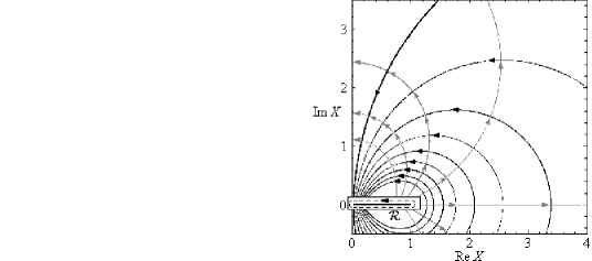
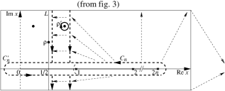
Figure 4: (at right) as fig. 3 but using the global variable $X\stackrel{{\scriptstyle\rm def}}{{=}}(x-{\textstyle{1\over 2}})/(2n)$ in the integral (45) (fig. 3 now fills the rectangle $\mathcal{R}$). Mathematica [37] contour plots for $\Phi(X)$ of (46): in black, deformed integration contours (level curves ${\{\mathop{\rm Re\,}\nolimits\Phi(X)=\Phi_{0}\}}$, $\Phi_{0}\downarrow 0^{+}$); in gray, steepest-descent lines (level curves of $\mathop{\rm Im\,}\nolimits\Phi$).

When zooming in to the $n\to\infty$, fixed-$x$ regime, then by (56) the level curves turn to parallel lines $\{\mathop{\rm Re\,}\nolimits x-{\textstyle{1\over 2}}=t_{0}\}$, and the deformation becomes ${t_{0}\to 0^{+}}$ (fig. 4 left). Only a portion of contour ${\mathcal{C}}_{n}^{\prime}\cap{\{\mathop{\rm Re\,}\nolimits x-{\textstyle{1\over 2}}<\varepsilon\}}$ escapes the deformation, but by (56) its contribution to the integral (45) is $O(n^{\varepsilon})$, ultimately negligible. Therefore, $\Lambda_{n}\pmod{o(R^{n})\ \forall R>\mathop{\rm e}\nolimits^{\Phi_{0}}}$ equals the above sum $\sum_{\rho^{\prime}}F_{n}(\rho^{\prime})$, which proves (49) under the replacement $R_{0}=\mathop{\rm e}\nolimits^{\Phi_{0}}$.

This fixed-$x$ regime actually governs each individual term of the sum (49): $F_{n}(\rho^{\prime})$ is the contribution to $\Lambda_{n}$ by a given zero $\rho^{\prime}$, that lives at a fixed $x$ ($\equiv{\textstyle{1\over 2}}+t+{\rm i}T\ (t>0)$). Therefore, setting $x=\rho^{\prime}$ in (56) directly delivers the asymptotic form (3.1) for $F_{n}(\rho^{\prime})$ which is explicit including the ${n\to\infty}$ dependence, as opposed to the exact $F_{n}(\rho^{\prime})$ specified via (43). Now (49), which is our other asymptotic ($n\to\infty$) statement, still uses exact $F_{n}(\rho^{\prime})$ that cannot be substituted outright by their explicit forms (3.1), because (3.1) is not asymptotic uniformly in $T$; it is nevertheless what describes $F_{n}(\rho^{\prime})$ for $n\to\infty$. Even more explicitly, using $|T|>T_{0}\gg 1$, $g(\rho^{\prime})\approx(2/|T|)^{t}\mathop{\rm e}\nolimits^{-{\rm sign}(T){\rm i}\pi/4}(2{\rm e}/|T|)^{{\rm i}T}$ (from the Stirling formula) leads to

$$F_{n}(\rho^{\prime})\approx\frac{1}{T^{2}\log n}\Bigl{(}\frac{2n}{|T|}\Bigr{)}^{t}(-1)^{n+1}\mathop{\rm e}\nolimits^{-{\rm sign}(T)\,{\rm i}\pi/4}\Bigl{(}\frac{2{\rm e}n}{|T|}\Bigr{)}^{{\rm i}T}\quad\mbox{for }n\gg|T|.$$ (57)

Thus, all in all, we needed two separate asymptotic formulae ((49)–(3.1)) to fully describe $\{\Lambda_{n}\}$ in the RH-false case.

If now RH is true then, as $\Phi_{0}$ attains $0^{+}$, (49) reaches no better than $\Lambda_{n}=o(R^{n})\ (\forall R>1)$, and only a finer analysis of the limiting integral on the critical line $L$ will lead to a definite asymptotic form, as follows.

3.3 Details for the case RH true

Here our quickest path is to adapt Oesterlé’s argument from §1.3.2.

To deform $\{\lambda_{n}\}$ into $\{\Lambda_{n}\}$, we replaced $[x/(x-1)]^{n}$ in (26) by $g_{n}(x)$ from (30). That changes (21) to

$$\Lambda_{n}=2\int_{0}^{\pi}\sin\Theta_{n}(\theta)\ N(T(\theta))\,{\rm d}\theta,\qquad T(\theta)\equiv{\textstyle{1\over 2}}\cot({\textstyle{1\over 2}}\theta),$$ (58)

where $\Theta_{n}(\theta)\in(0,n\pi]$ ($\equiv n\theta$ previously for $\lambda_{n}$) is now the sum of the $n$ angles subtended by the real vectors $(\overrightarrow{1-2m,2m})$ from the point ${\textstyle{1\over 2}}+{\rm i}T(\theta)$, for $m=1,2,\ldots,n$. Namely,

$$\Theta_{n}(\theta)=2\sum_{m=1}^{n}\arctan\Bigl{[}(4m-1)\tan({\textstyle{1\over 2}}\theta)\Bigr{]}:\quad[0,\pi]\mapsto[0,n\pi].$$ (59)

The two endpoint slopes of the function $\Theta_{n}(\theta)$ will then play key roles:

$$\Theta_{n}^{\prime}(0)\!\!\! = \!\!\!\sum_{m=1}^{n}(4m-1)\equiv n(2n+1),$$ (60)

$$\Theta_{n}^{\prime}(\pi)\!\!\! = \!\!\!\sum_{m=1}^{n}(4m-1)^{-1}\equiv{\textstyle{1\over 4}}\bigl{[}\psi(n+{\textstyle{3\over 4}})+\gamma+3\log 2-\pi/2\bigr{]}$$ (61)

$$= \!\!\!\min_{[0,\pi]}\Theta_{n}^{\prime}(\theta)\qquad\mbox{ because }\Theta_{n}^{\prime}(\theta)>0,\ \Theta_{n}^{\prime\prime}(\theta)<0\mbox{ on }[0,\pi]$$ (62)

(all resulting from (59) term by term; we denote ${}^{\prime}\equiv\frac{\mbox{\small${\rm d}$}}{\mbox{\small${\rm d}\theta$}}$, $\psi(x)\equiv\frac{\mbox{\small${\rm d}$}}{\mbox{\small${\rm d}x$}}\log\Gamma(x)$).

We then follow the same steps as with (21) for $\lambda^{\rm K}_{n}$ in § 1.3.2, now plugging $N({\textstyle{1\over 2}}\cot{\textstyle{1\over 2}}\theta)=-(2\pi\theta)^{-1}\log(2\pi{\rm e}\,\theta)+O(|\log\theta|)_{\theta\to 0^{+}}$ from (22) into (58).

1) $O(|\log\theta|)$ will be negligible as before if the derivation of the Riemann–Lebesgue lemma [28, § 5.14] extends so as to prove

$$I_{n}(f)\stackrel{{\scriptstyle\rm def}}{{=}}\int_{0}^{\pi}\sin\Theta_{n}(\theta)\,f(\theta)\,{\rm d}\theta=o(1)_{n\to\infty}\ \mbox{ for any $f$ integrable on }[0,\pi].$$ (63)

Now $C^{1}$ functions are dense in $L^{1}$, [28, thm 3.14] so for any $\varepsilon>0$ there exists ${\mathbf{f}}\in C^{1}[0,\pi]$ such that $\|f-{\mathbf{f}}\|_{L^{1}}<\varepsilon$, then it remains to prove $|I_{n}({\mathbf{f}})|<\varepsilon$ for $n$ large enough, i.e., $I_{n}({\mathbf{f}})=o(1)_{n\to\infty}$. We integrate by parts in the variable $\Theta_{n}$:

$$I_{n}({\mathbf{f}})\!\!\! = \!\!\!\int_{0}^{n\pi}\!\!\sin\Theta_{n}\Bigr{[}{\mathbf{f}}(\theta(\Theta_{n}))\frac{{\rm d}\theta}{{\rm d}\Theta_{n}}\Bigr{]}{\rm d}\Theta_{n}=\Bigr{[}\!\!-\cos\Theta_{n}\,{\mathbf{f}}(\theta(\Theta_{n}))\frac{{\rm d}\theta}{{\rm d}\Theta_{n}}\Bigr{]}_{0}^{n\pi}\!+J_{n},$$ (64)

$$J_{n}\!\!\! \stackrel{{\scriptstyle\rm def}}{{=}} \!\!\!\int_{0}^{n\pi}\!\!\cos\Theta_{n}\,\frac{{\rm d}}{{\rm d}\Theta_{n}}\Bigr{[}{\mathbf{f}}(\theta(\Theta_{n}))\frac{{\rm d}\theta}{{\rm d}\Theta_{n}}\Bigr{]}{\rm d}\Theta_{n}=J_{n}^{(1)}+J_{n}^{(2)},$$

$$J_{n}^{(1)}\!\!\! = \!\!\!\int_{0}^{n\pi}\!\!\cos\Theta_{n}\,{\mathbf{f}}^{\prime}(\theta(\Theta_{n}))\Bigl{(}\frac{{\rm d}\theta}{{\rm d}\Theta_{n}}\Bigr{)}^{\!2}{\rm d}\Theta_{n}\equiv\int_{0}^{\pi}\!\cos\Theta_{n}(\theta)\,{\mathbf{f}}^{\prime}(\theta)\frac{1}{\Theta^{\prime}_{n}(\theta)}\,{\rm d}\theta,$$

$$J_{n}^{(2)}\!\!\! = \!\!\!\int_{0}^{n\pi}\!\!\cos\Theta_{n}\,{\mathbf{f}}(\theta(\Theta_{n}))\frac{{\rm d}^{2}\theta}{{\rm d}\Theta_{n}^{2}}\,{\rm d}\Theta_{n}=\cos\Theta_{n}^{(0)}\,{\mathbf{f}}(\theta(\Theta_{n}^{(0)}))\Bigl{[}\frac{{\rm d}\theta}{{\rm d}\Theta_{n}}\Bigr{]}_{0}^{n\pi}\!,\ \Theta_{n}^{(0)}\in[0,\pi]$$

for some $\Theta_{n}^{(0)}$, by the first mean-value theorem [17, § 12.111] (with ${\rm d}^{2}\theta/{\rm d}\Theta_{n}^{2}\equiv-\Theta_{n}^{\prime\prime}/{\Theta_{n}^{\prime}}^{3}$ not changing sign, from (62)). Now (61) entails $\Theta_{n}^{\prime}(\pi)\sim{\textstyle{1\over 4}}\log n$ upon which (62) implies ${\rm d}\theta/{\rm d}\Theta_{n}\equiv 1/\Theta_{n}^{\prime}(\theta)=O(1/\log n)$ uniformly. Then $J_{n}^{(1)},J_{n}^{((2)}$ are $O(1/\log n)$ from their respective rightmost expressions above, hence so are $J_{n}$ and finally $I_{n}({\mathbf{f}})$ in (64), which ensures $I_{n}({\mathbf{f}})=o(1)$. $\square$

2) For the main term $-\int_{0}^{\pi}\sin\Theta_{n}(\theta)\,(\pi\theta)^{-1}\log(2\pi{\rm e}\,\theta)\,{\rm d}\theta$ in (58): by (63), only the nonintegrable singularity multiplying $\sin\Theta_{n}$ should matter (i.e., ${\theta=0}$); here $\Theta_{n}(\theta)\sim\Theta_{n}^{\prime}(0)\,\theta$, vs $n\theta$ previously, so it must suffice to substitute $\Theta_{n}^{\prime}(0)=n(2n+1)$ for $n$ in the previous result (24) for $\lambda_{n}^{\rm K}$, to get

$$\Lambda_{n}\sim{\textstyle{1\over 2}}\log\Theta_{n}^{\prime}(0)+c={\textstyle{1\over 2}}\log\,[n(2n+1)]+c\sim\log n+(c+{\textstyle{1\over 2}}\log 2).$$ (65)

And the intermediate results to replace (23) must be

$${\mathcal{I}}_{0,n}\!\!\! = \!\!\!\int_{0}^{\pi}\sin\Theta_{n}\frac{{\rm d}\theta}{\theta}={\textstyle{1\over 2}}\pi+o(1)_{n\to\infty}\,,$$ (66)

$${\mathcal{I}}_{1,n}\!\!\! = \!\!\!\int_{0}^{\pi}\sin\Theta_{n}\log\theta\,\frac{{\rm d}\theta}{\theta}=-{\textstyle{1\over 2}}\pi\,(\log\,[n(2n+1)]+\gamma)+o(1)_{n\to\infty}\,,$$ (67)

which can be checked numerically (through nonarithmetical tests), and indeed combine in (58) to yield (65): i.e., the targeted result (3.1).

Now a technicality arises: (30) obviously implies

$$\mathop{\rm e}\nolimits^{-{\rm i}\Theta_{n}(\theta)}\equiv g_{n}({\textstyle{1\over 2}}+{\rm i}T(\theta))\qquad(\mbox{recalling }T(\theta)\equiv{\textstyle{1\over 2}}\cot{\textstyle{1\over 2}}\theta),$$ (68)

so the function $\Theta_{n}$ also has the two disjoint nonuniform $n\to\infty$ regimes of $g_{n}$: (52) for $\theta=O(1/n)$ vs (55) for fixed but nonzero $\theta$, and this complicates a rigorous rewording of the above heuristics, as done next. (We have quicker proofs for (66) alone.)

We then shift focus onto a parametric integral, ${\mathcal{I}}_{n}(\alpha)\stackrel{{\scriptstyle\rm def}}{{=}}\int_{0}^{\pi}\sin\Theta_{n}\,{\rm d}\theta/\theta^{\alpha}$ (for $\alpha<1$), which in the end will restore ${\mathcal{I}}_{q,n}\equiv(-{\rm d}/{\rm d}\alpha)^{q}\,{\mathcal{I}}_{n}(\alpha=1^{-})$ for $q=0,1$. But to better benefit from complex contour deformations, we prefer integrals without endpoints: with $\theta$ being an angle, such are

$${\mathcal{I}}_{\pm,n}(\alpha)\stackrel{{\scriptstyle\rm def}}{{=}}\int_{-\pi}^{\pi}g_{n}({\textstyle{1\over 2}}+{\rm i}T(\theta))(\mathop{\rm e}\nolimits^{\pm{\rm i}\pi/2}\theta)^{-\alpha}\,{\rm d}\theta,$$ (69)

where the standard determination (cut along ${\mathbb{R}}^{-}$) is taken for $v\mapsto v^{-\alpha}$. The identity (68) extends to $[-\pi,\pi]$ with $\Theta_{n}(-\theta)=-\Theta_{n}(\theta)$, which actually makes $\mathop{\rm e}\nolimits^{-{\rm i}\Theta_{n}(\cdot)}$ a regular function of $\theta\in{\mathbb{R}}/2\pi{\mathbb{Z}}$, hence also $g_{n}({\textstyle{1\over 2}}+{\rm i}T(\cdot))$. Then by inspection, ${\mathcal{I}}_{\pm,n}(\alpha)\equiv 2\int_{0}^{\pi}\cos[\Theta_{n}(\theta)\pm{\textstyle{1\over 2}}\pi\alpha]\,{\rm d}\theta/\theta^{\alpha}$, in turn implying

$${\mathcal{I}}_{n}(\alpha)\equiv\frac{1}{4\sin{\textstyle{1\over 2}}\pi\alpha}[{\mathcal{I}}_{-,n}(\alpha)-{\mathcal{I}}_{+,n}(\alpha)].$$ (70)

Now (69) is controllable for $n\to\infty$ by the steepest-descent method: we deform its real integration cycle ($\{|g_{n}|=1\}$) to level lines ${\{|g_{n}|={\rm const.}<1\}}$ in the complex domain, $\{\theta-{\rm i}u_{\theta}\mid\theta\in{\mathbb{R}}/2\pi{\mathbb{Z}}\}$, $u_{\theta}>0$ due to $\Theta^{\prime}_{n}(\theta)>0$. (This is, viewed in the $\theta$-variable, just the deformation of § 3.2 but taken beyond the imaginary $X$-axis.) Since moreover $\Theta^{\prime}_{n}(\theta)\to+\infty$ uniformly, barely deformed level curves (such that $u_{\theta}\sim\sqrt{\log n}/\Theta^{\prime}_{n}(\theta)=o(1)$ uniformly) reach $|g_{n}|=o(1)$ save for obstructions to that lowering of the path, of which there may be three. First, singularities of the function $\Theta_{n}(\theta)$, but the nearest one is $(-2\arctan[1/(4n-1)]\ {\rm i})$, and $|g_{n}|=o(1)$ is achieved far above. Then, the jump we call $h(u)$ of the nonperiodic factor $\theta^{-\alpha}$ in (69) across the line ${\{\pi-{\rm i}u\pmod{2\pi}\mid u\in{\mathbb{R}}\}}$: its contribution to ${\mathcal{I}}_{\pm,n}(\alpha)$ has size $|\!\int_{0}^{u_{\pi}}g_{n}({\textstyle{1\over 2}}+{\rm i}T(\pi-{\rm i}u))\,h(u)\,{\rm d}u\,|\sim|\!\int_{0}^{u_{\pi}}g({\textstyle{1\over 2}}-{\textstyle{1\over 4}}u)\,h(u)\,n^{-u/4}{\rm d}u\,|$ using ${T(\pi-{\rm i}u)}\equiv{\textstyle{1\over 2}}\cot{\textstyle{1\over 2}}(\pi-{\rm i}u)\sim{\textstyle{1\over 4}}{\rm i}u$ then (55) (the regime of § 3.1.2 holds as $T\approx 0$); now both $g(\cdot)$ and $h$ are regular functions in $u$ hence the last integral, by the Laplace method as in § 3.1.2, is $O(1/\log n)=o(1)$. Finally, the sole obstacle of consequence is the cut of $(\pm{\rm i}\theta)^{-\alpha}$ from $\theta=0$ but for $(+{\rm i}\theta)^{-\alpha}$, even that cut goes upwards (out of the way), resulting in ${\mathcal{I}}_{+,n}(\alpha)=o(1)$. Whereas for ${\mathcal{I}}_{-,n}(\alpha)$, the cut is downward: ${\{\theta=-{\rm i}u\mid u>0\}}$, and it contributes

$${\mathcal{I}}_{-,n}(\alpha)\sim(\mathop{\rm e}\nolimits^{+{\rm i}\pi\alpha}-\mathop{\rm e}\nolimits^{-{\rm i}\pi\alpha})\int_{0}^{u_{0}}\mathop{\rm e}\nolimits^{-{\rm i}\Theta_{n}(-{\rm i}u)}\frac{(-{\rm i}\,{\rm d}u)}{u^{\alpha}}=2\sin\pi\alpha\int_{0}^{u_{0}}\mathop{\rm e}\nolimits^{-{\rm i}\Theta_{n}(-{\rm i}u)}\frac{{\rm d}u}{u^{\alpha}}.$$ (71)

Since $|u|\leq u_{0}\sim\frac{\mbox{\small$\sqrt{\log n}$}}{\mbox{\small$n(2n+1)$}}=o(1/n)$, we rescale $\tau\equiv 2nu\ (=o(1))$. Now from (68), $\mathop{\rm e}\nolimits^{-{\rm i}\Theta_{n}(-{\rm i}u)}\sim g_{n}({\textstyle{1\over 2}}-2n/\tau)\sim(\frac{1-\tau}{1+\tau})^{1/4}\mathop{\rm e}\nolimits^{n\Phi(-1/\tau)}$ using $T(-{\rm i}u)\sim{\rm i}/u=2n{\rm i}/\tau$ then (52) (the regime of § 3.1.1 holds as $|T|\gg n$). Add that $\Phi(-1/\tau)\sim-\tau$ ($\tau\approx 0$), and the integrand in (71) begs for the Laplace method as in § 3.1.1. Applied directly on (71), this gives $\int_{0}^{u_{0}}\mathop{\rm e}\nolimits^{-{\rm i}\Theta_{n}(-{\rm i}u)}u^{-\alpha}{\rm d}u\sim\mathop{\rm e}\nolimits^{-{\rm i}\Theta_{n}(0)}\int_{0}^{\infty}\mathop{\rm e}\nolimits^{-\Theta^{\prime}_{n}(0)\,u}[u^{-\alpha}+O(u^{1-\alpha})]{\rm d}u=\Gamma(1-\alpha)\,[n(2n+1)]^{\alpha-1}+O(n^{2(\alpha-2)})$, resulting in

$${\mathcal{I}}_{-,n}(\alpha)=\frac{2\pi}{\Gamma(\alpha)}[n(2n+1)]^{\alpha-1}+O(n^{2(\alpha-2)}).$$ (72)

Finally then, recalling (70) and ${\mathcal{I}}_{+,n}(\alpha)=o(1)$,

$${\mathcal{I}}_{q,n}(\alpha)\sim\Bigl{(}-\frac{{\rm d}}{{\rm d}\alpha}\Bigr{)}^{q}\Bigr{[}\frac{1}{4\sin{\textstyle{1\over 2}}\pi\alpha}\,{\mathcal{I}}_{-,n}(\alpha)\Bigr{]}_{\alpha=1}\pmod{o(1)}$$ (73)

with $q=0$, resp. 1, yield (66), resp. (67), and consequently (65). (All the above remainders are uniform and differentiable in $\alpha$ up to $\alpha=1$.) $\square$

3.4 Asymptotic or full-fledged Li’s criterion for $\{\Lambda_{n}\}$?

(a heuristic parenthesis).

A full Li’s crterion for the new sequence $\{\Lambda_{n}\}$ would be

$$\qquad\mbox{RH}\quad\iff\quad\Lambda_{n}>0\ \mbox{ for all }n\qquad\mbox{(unproven)};$$

while we lack a proof encompassing all $n$, this is not essential in our focus on RH-sensitivity: already for $\{\lambda_{n}\}$, only $n\gg 1$ truly counted (§ 1.2); and likewise here, our criterion (49)–(3.1) entails $\Lambda_{n}>0$ asymptotically if and only if RH holds (fig. 9 will illustrate that on a counterexample to RH).

As for lower $n$, $\Lambda_{n}>0$ will be numerically manifest there (see § 4.1).

All those facts still let us conjecture that Li’s criterion fully holds for the sequence $\{\Lambda_{n}\}$ as well (but we deem it harder to prove than for $\{\lambda_{n}\}$).

3.5 Generalized-RH asymptotic alternative

All previous developments carry over from $\zeta(x)$ to some Dirichlet L-functions: those of the form

$$L_{\chi}(x)\stackrel{{\scriptstyle\rm def}}{{=}}\sum_{k=1}^{\infty}\frac{\chi(k)}{k^{x}}\equiv d^{-x}\sum_{k=1}^{d}\chi(k)\,\zeta(x,k/d),$$ (74)

where $\chi$ is a special type of $d$-periodic function on ${\mathbb{Z}}$ ($d>1$): a real primitive Dirichlet character ($\chi$ then has a definite parity, even or odd) [11, chaps. 5–6]; $\zeta(x,w)$ is the Hurwitz zeta function [11, chap. 9 eq. (16)]). Such $L_{\chi}(x)$ have very close properties to Riemann’s $\zeta(x):$

• Functional equations: [2, App. B, Thm B.7 & eq.(46)] (real primitive $\chi$ are Kronecker symbols, for which the usual Gaussian-sum factor $\varepsilon(\chi)\equiv 1$)

$$\xi_{\chi}(x)\stackrel{{\scriptstyle\rm def}}{{=}}(\pi/d)^{-x/2}\Gamma\bigl{(}{\textstyle{1\over 2}}(x\!+\!b)\bigr{)}\,L_{\chi}(x)\equiv\xi_{\chi}(1-x),\quad b=\biggl{\{}\matrix{0\ \ (\chi\mbox{ even})\cr 1\ \ (\chi\mbox{ odd})\hfill}\biggr{\}}.$$ (75)

• Explicit values at integers, in terms of Bernoulli polynomials: by the classic identities $(\ell+1)\,\zeta(-\ell,a)=-B_{\ell+1}(a)$ ($\ell=0,1,2,\ldots$), (74) makes $L_{\chi}(x)$ explicit at all $x=-\ell$; the functional equation (75) then converts that to explicit values for $L_{\chi}$ (and $\xi_{\chi}$) at all even, resp. odd, positive integers according to the even, resp. odd parity of $\chi$. Moreover, $L_{\chi}(1)$ (hence $\xi_{\chi}(1)$) is explicitly computable also for even parity [11, chap. 1][34, eq.(10.70)].

• Generalized Riemann Hypothesis (GRH): all zeros $\rho$ of $\xi_{\chi}$ have $\mathop{\rm Re\,}\nolimits\rho={\textstyle{1\over 2}}$.

• A Keiper–Li sequence $\{\lambda_{\chi,n}\}$ exists for $\xi_{\chi}$ in full similarity to $\{\lambda_{n}\}$ for $\xi$ (applying [8, Cor. 1]). For GRH, the only change in our asymptotic alternative (1.2)–(1.2) affects the constant $c$ in (1.2) or (24) due to the replacement, in the asymptotic counting function $\overline{N}(T)$ from (3) used in § 1.3.2, of the term $\log(T/\,2\pi{\rm e})$ by $\log(Td/\,2\pi{\rm e})$ [11, chap. 16], which results in

$$\mbox{GRH true: }\quad\lambda^{\rm K}_{\chi,n}\sim{\textstyle{1\over 2}}\log n+c_{d}\pmod{o(1)},\qquad c_{d}=c+{\textstyle{1\over 2}}\log d.$$ (76)

Then as in § 2.1, we can discretize the definition of $\{\lambda^{\rm K}_{\chi,n}\}$ to get an explicit sequence $\{\Lambda_{\chi,n}\}$ involving finite differences of elementary $\log\xi_{\chi}$-values. For even $\chi$, everything stays as in § 2.1 (where even parity is implied throughout), hence $\Lambda_{\chi,n}$ are given by (36) with $2\,\xi(2m)$ simply replaced by $\frac{\mbox{\small$1$}}{\mbox{\small$\xi_{\chi}(1)$}}\,\xi_{\chi}(2m)$. For odd $\chi$ on the other hand, the points $x_{m}$ have to be relocated from $2m$ to $2m+1$, resulting in these main changes:

$$[(\ref{gdf})\to]\qquad g^{\rm odd}_{n}(x)\stackrel{{\scriptstyle\rm def}}{{=}}\prod_{m=1}^{n}\frac{x+2m}{x-2m-1}\!\!\! \equiv \!\!\!g^{\rm odd}(x)(-1)^{n}\frac{\Gamma({\textstyle{1\over 2}}x+1+n)}{\Gamma({\textstyle{1\over 2}}(3\!-\!x)\!+\!n)},$$

$$g^{\rm odd}(x)\!\!\! \stackrel{{\scriptstyle\rm def}}{{=}} \!\!\!\frac{-\sqrt{\pi}\,2^{x-1}}{\cos(\pi x/2)\,\Gamma(x)},$$ (77)

$$[(\ref{Anm})\to]\qquad A^{\rm odd}_{nm}=2^{-2n}(n+m,n-m,2m+1)!\,/(2m+1),\qquad\qquad$$ (78)

$$[(\ref{Fdef})\to]\quad F^{\rm odd}_{n}(x)=(-1)^{n}\biggl{[}\frac{-1}{A^{\rm odd}_{n0}}\log x+\sum_{m=0}^{n}(-1)^{m}A^{\rm odd}_{nm}\log(x\!-\!2m\!-\!1)\biggr{]},$$ (79)

$$[(\ref{EKL})\to]\quad\Lambda_{\chi,n}\equiv(-1)^{n}\sum_{m=1}^{n}(-1)^{m}A^{\rm odd}_{nm}\log\biggl{[}\frac{1}{\xi_{\chi}(1)}\xi_{\chi}(2m\!+\!1)\biggr{]}\ \ (\chi\mbox{ odd}).$$ (80)

All in all, the asymptotic alternative (49)–(3.1) generalizes to one depending on $\chi$, via its parity for GRH false, and period $d$ for GRH true:

$$\bullet\mbox{ GRH false: }\Lambda_{\chi,n}\!\!\! \sim \!\!\!\!\!\sum_{\rho^{\prime}-\frac{1}{2}\,\in\,2n\,{\mathcal{D}}_{R_{0}}}\!\!F^{\#}_{n}(\rho^{\prime})\pmod{o(R^{n})\ \forall R>R_{0}>1}\quad$$ (81)

and, $$\!\!\!\!\!\!\mbox{for each given GRH-violating zero }\rho^{\prime},$$

$$F^{\#}_{n}(\rho^{\prime})\!\!\! \sim \!\!\!\frac{g^{\#}(\rho^{\prime})}{\rho^{\prime}(\rho^{\prime}-1)}(-1)^{n}\frac{n^{\rho^{\prime}-\frac{1}{2}}}{\log n}\quad(n\to\infty),$$ (82)

$$\mbox{with}\quad(F^{\#}_{n},g^{\#})\!\!\! \stackrel{{\scriptstyle\rm def}}{{=}} \!\!\!\biggl{\{}\matrix{(F_{n},\quad g)&\mbox{for $\chi$ even, cf. (\ref{Fdef}), (\ref{gdf})}\cr(F^{\rm odd}_{n},g^{\rm odd})&\mbox{for $\chi$ odd, \ cf. (\ref{Fodd}), (\ref{G-df})}}\biggr{\}};$$ (83)

$$\bullet\mbox{ GRH true: }\Lambda_{\chi,n}\!\!\! \sim \!\!\!\log n+C_{d}\pmod{o(1)},\qquad C_{d}=C+{\textstyle{1\over 2}}\log d$$ (84)

($\equiv c_{d}+{\textstyle{1\over 2}}\log 2$), cf. (3.1), (76).

Remark: for a Siegel zero if any ($T=0$), (82) simply gives $F^{\#}_{n}(\rho^{\prime})\propto\frac{\mbox{\small$(-1)^{n}n^{t}$}}{\mbox{\small$\log n$}}$.

4 Quantitative aspects

We now discuss how the discretized Keiper sequence $\{\Lambda_{n}\}$ vs the Keiper–Li $\{\lambda_{n}\}$ might serve as a practical probe for RH in a complementary perspective to standard tests. (To rigorously (dis)prove RH using $\{\Lambda_{n}\}$ is also a prospect in theory, but we have not explored that.)

4.1 Numerical data in the Riemann case

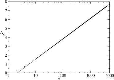
Figure 5: The coefficients $\Lambda_{n}$ computed by (36) up to $n=4000$, on a logarithmic $n$-scale. (On all plots, the line segments in gray connect data points only to aid the eye.) Straight line: the RH-true asymptotic form (3.1), $(\log n+C)$.

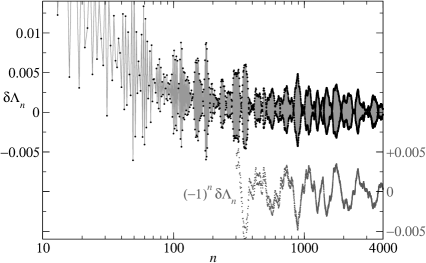
Figure 6: The remainder sequence $\delta\Lambda_{n}=\Lambda_{n}-(\log n+C)$, and a rectified form $(-1)^{n}\delta\Lambda_{n}$ (drawn for $n>300$, shifted downwards for clarity) to cancel the period-2 oscillations of $\delta\Lambda_{n}$ at large $n$.

Low-$n$ calculations of $\Lambda_{n}$ (fig. 5) agree very early with our predicted RH-true behavior (here, (3.1)), just as they did for $\lambda_{n}$ [19][22] and for the same reason: given the current value $T_{0}\approx 2.4\cdot 10^{12}$ up to which RH is verified, an imprint (57) by an RH-violating zero $\rho^{\prime}$ might be of visible size only beyond some much higher $n$-value. Explicit $n$-thresholds as functions of $\rho^{\prime}$ will be tackled below in § 4.2–4.3 (but with no unique answer like (17) for $\{\lambda_{n}\}$).

The remainder term $\delta\Lambda_{n}\stackrel{{\scriptstyle\rm def}}{{=}}\Lambda_{n}-(\log n+C)$ looks compatible with an $o(1)$ bound (fig. 6), albeit less neatly than the analogous $\delta\lambda^{\rm K}_{n}$ [19, fig. 1][22, fig. 6b] (note: even Keiper [19] plotted $\delta\lambda^{\rm L}_{n}=n\ \delta\lambda^{\rm K}_{n}$). For the record,

$$\Lambda_{1}\!\!\! \approx \!\!\!0.069176395771,\ \ \Lambda_{2}\approx 0.22745427267,\ \ \Lambda_{3}\approx 0.45671413349;\ \ (\mbox{cf. }(\ref{ExV}))$$

$$n\!\!\! = \!\!\!\ \ 2000:\quad\Lambda_{n}\approx 6.815360445451163\quad(\delta\Lambda_{n}\approx-0.0017849),$$

$$n\!\!\! = \!\!\!\ 10000:\quad\Lambda_{n}\approx 8.428662659671506\quad(\delta\Lambda_{n}\approx+0.0020794),$$

$$n\!\!\! = \!\!\!\ 20000:\quad\Lambda_{n}\approx 9.119244876955247\quad(\delta\Lambda_{n}\approx-0.000485565),$$ (85)

$$n\!\!\! = \!\!\!100000:\quad\Lambda_{n}\approx 10.729678153023\quad(\delta\Lambda_{n}\approx+0.0005097985),$$

$$n\!\!\! = \!\!\!200000:\quad\Lambda_{n}\approx 11.42244991847\quad(\delta\Lambda_{n}\approx+0.0001343834)$$

$$n\!\!\! = \!\!\!500000:\quad\Lambda_{n}\approx 12.33812102688\quad(\delta\Lambda_{n}\approx-0.0004852401)$$

($n>20000$ samples: courtesy of G. Misguich [25], see § 4.5).

The main oscillation in $(-1)^{n}\delta\Lambda_{n}$ (fig. 6) must come from $F_{n}(\rho_{1})$ in (44) for the lowest Riemann zero $\rho_{1}:$ the $(\log n)$-period agrees with $2\pi/\mathop{\rm Im\,}\nolimits\rho_{1}$ (per the asymptotic form (56)), as $2\pi/14.1347\approx 0.44\,$.

4.2 Putative imprints of zeros violating RH

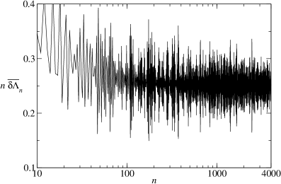
Figure 7: The averaged remainder sequence (88) rescaled by $n$, namely: $n\,\overline{\delta\Lambda}_{n}\,$. (Some further values: $0.27027$ for $n=10000,\ 0.23970$ for $n=20000,\ 0.2559$ for $n=100000,\ 0.2683$ for $n=200000,\ 0.27957$ for $n=500000$ [25].)

RH-violating zeros $\rho^{\prime}$ (if any) seem to enter the picture just as for $\{\lambda_{n}\}$: their contributions (3.1) will asymptotically dominate $\log n$ from (3.1), but numerically they will emerge and take over extremely late. Indeed for such a zero $\rho^{\prime}={{\textstyle{1\over 2}}+t+{\rm i}T}$, with $0<t<{\textstyle{1\over 2}}$ and $T\gtrsim 2.4\cdot 10^{12}$ [16], its contribution (57) scales as $T^{-2}(2n/T)^{t}/\log n$ in modulus. We then get a manifest or “naive” crossover threshold (in order of magnitude, neglecting logarithms and constants against powers) by solving

$$T^{-2}(n/T)^{t}\!\!\! \approx \!\!\!1$$ (86)

$$\Longrightarrow\qquad n\!\!\! \gtrsim \!\!\!T^{1+2/t}\qquad(\mbox{best case: }O(T^{5+0})\mbox{ for }t={\textstyle{1\over 2}}-0).$$ (87)

This is worse than (18) for $\lambda_{n}$, all the more if $\Lambda_{n}<0$ were sought (the right-hand side of (86) should then be $\log^{2}n$). However, (86) is a sufficient but not necessary condition, which leaves room for possible improvement. The core problem is to filter out a weak $\rho^{\prime}$-signal from the given background (3.1), therefore any predictable structure in the latter is liable to boost the gain. For instance, the hyperfine structure of $\delta\Lambda_{n}$ is oscillatory of period 2 (fig. 6); this suggests to average over that period, which empirically discloses a rather neat $(1/n)$-decay trend (fig. 7):

$$\overline{\delta\Lambda}_{n}\stackrel{{\scriptstyle\rm def}}{{=}}{\textstyle{1\over 2}}(\delta\Lambda_{n}+\delta\Lambda_{n-1})\approx 0.25/n.$$ (88)

The same averaging on a $\rho^{\prime}$-signal $F_{n}(\rho^{\prime})$ in (3.1) roughly applies ${\textstyle{1\over 2}}({\rm d}/{\rm d}n)$ to the factor $n^{T}$ therein (again neglecting $t\ll T$ and $\log n$), i.e., multiplies it by ${\textstyle{1\over 2}}(T/n)$. Thus heuristically, i.e., conjecturing the truth of (88) for $n\to\infty$ under RH, the crossover condition improves from (86) to

$$(T/n)\,T^{-2}(n/T)^{t}\!\!\! \approx \!\!\!\overline{\delta\Lambda}_{n}\approx 1/n$$

$$\Longrightarrow\quad n\!\!\! \gtrsim \!\!\!T^{1+1/t}\ (\mbox{best case: }O(T^{3+0})\mbox{ for }t={\textstyle{1\over 2}}-0).\quad$$ (89)

We can hope that more selective signal-extraction schemes may still lower this detection threshold. Even an empirical mindset may be acceptable there: the $\{\Lambda_{n}\}$ (like $\{\lambda_{n}\}$) should anyway work best for global coarse detection of a possible RH-violation (as discussed in more detail in the next §).

4.3 The uncertainty principle for $\{\Lambda_{n}\}$

An absolute detection limit is however provided by the uncertainty principle, and this has to be quantified here. Near the critical line $\{\mathop{\rm Re\,}\nolimits X=0\}$ parametrized by $U\stackrel{{\scriptstyle\rm def}}{{=}}\mathop{\rm Im\,}\nolimits X$, and for large $n$, $\Lambda_{n}$ is an integral of the zeros’ distribution against essentially $\mathop{\rm e}\nolimits^{{\rm i}n\Psi(U)}$ (by (45), (54), (48)): i.e., a high-frequency distorted plane wave. Then, to resolve $t>0$ for a zero $\rho^{\prime}={{\textstyle{1\over 2}}+t+{\rm i}T}\equiv{\textstyle{1\over 2}}+2nX$, the uncertainty principle asks its scale ($\mathop{\rm Re\,}\nolimits X=t/(2n)$ in the $X$-plane) to exceed the inverse of the local wavenumber for $\mathop{\rm e}\nolimits^{{\rm i}n\Psi(U)}$ which is $n\,{\rm d}\Psi/{\rm d}U$, or ${n\log(1+1/U^{2})}$ using (46), with $U=\mathop{\rm Im\,}\nolimits X=T/(2n):$ that means ${{\textstyle{1\over 2}}t\,\log(1+4n^{2}/T^{2})}\gtrsim 1$ or, to a fair approximation when $t<{\textstyle{1\over 2}}$,

$$n\gtrsim{\textstyle{1\over 2}}\,|T|\mathop{\rm e}\nolimits^{1/t}.$$ (90)

Against the corresponding bound (17) for $\{\lambda_{n}\}$ ($n\gtrsim T^{2}/t$), (90) will at any given $t>0$ favor $\{\Lambda_{n}\}$ once $|T|\gtrsim{\textstyle{1\over 2}}t\mathop{\rm e}\nolimits^{1/t}$. E.g., at the current floor height (1), the best possible $n$-threshold (i.e., for $t={\textstyle{1\over 2}}-0$) gets improved to $10^{13}$ (possibly reachable?), from $10^{25}$ for $\{\lambda_{n}\}$ in (18). The bound (90) also allows $n$ to go well below the “naive” detection threshold (87) and even (4.2) - in principle: (90) is a necessary but not sufficient condition, and there still remains to actually see the $\rho^{\prime}$-signal, very weak at such decreased $n$, amidst the “noise” $\delta\Lambda_{n}$ brought into (44) by the many more nearby zeros that are on the critical line.

That $\rho^{\prime}$-signal, precisely (57) plus its complex-conjugate (from ${\rho^{\prime}}^{\ast}$), is $(-1)^{n}\times$ a growing oscillation of frequency $T/\,2\pi$ in the variable ($\log n$) (such as plotted on fig. 9, a later counterexample to $\mathop{\rm Re\,}\nolimits\rho\equiv{\textstyle{1\over 2}}$). From $n$ high enough as in (87) (e.g., $\gtrsim 100$ in fig. 9) this signal will overwhelmingly grow, and a single $\Lambda_{n}$ will (most likely) betray it as evidence of an RH-violating zero somewhere, with only (87) (read backwards) to narrow its localization. Detection by shape-matching with (57) should be more precise, thus permit lower $n$-values (where the $\rho^{\prime}$-signal is weaker) at the cost of using a range of $n$. Better knowledge of the structure and true size of the $o(1)$ “noise” in (3.1) would be a key factor to neater results. Barring that, we only risk highly intuitive and tentative guesswork for a buried $\rho^{\prime}$-signal. The $n$-variable is Fourier-conjugate to the $\Psi$-coordinate on the critical line $\{\mathop{\rm Re\,}\nolimits X=0\}$; then the Heisenberg inequality (again) roughly bounds the localization (uncertainty) on $\Psi$ as $\Delta\Psi\gtrsim 1/\Delta n$ where $\Delta n$ is the $n$-interval on which the signal ($\Lambda_{n}$) is probed; computing as above reduces that to $\Delta U\gtrsim\log(1+1/U^{2})/\Delta n$ or, to a fair approximation under (90),

$$\Delta T\gtrsim 4\log\frac{2n}{T}\,\frac{n}{\Delta n}\quad\Bigl{(}\gtrsim\frac{2T}{t}\,\frac{\mathop{\rm e}\nolimits^{1/t}}{\Delta n}\mbox{ by (\ref{UPL})}\Bigr{)}.$$ (91)

The best localization of $T$ thus improves as the width of the $n$-region grows.

All that is clearly complementary to the direct (Riemann–Siegel based) verification methods, which are local in $T$ [16]. These are fully rigorous, computationally more efficient, but strictly confined to the $T$-region on which they are applied (thus their actual cost of use may still skyrocket if the region to be searched is unbounded). Like $\{\lambda_{n}\}$ but more easily, $\{\Lambda_{n}\}$ offers a “dual” global viewpoint: it could lead in fewer steps to a suspicion of an RH-violating zero (if any) but neither rigorously nor very sharply, nevertheless enough to hint at a smaller region, in which a direct algorithm [16] could then faster and in full rigor confirm (or disprove) that violation of RH.

4.4 The Davenport–Heilbronn counterexamples

More tests of interest require the generalization of § 3.5 to odd parity. Among Dirichlet L-functions we only tested the $\beta$-function (of period 4) and saw no difference of behavior patterns in $\{\Lambda_{\beta,n}\}$ vs $\{\Lambda_{n}\}$. If we then go beyond, there exist special Dirichlet series that are not Dirichlet L-functions, but obey similar functional equations and have many zeros off the critical line $L$ [12][32, § 10.25][31][4][7, § 5]. In those we may seek a testing ground for the RH-false branch of our asymptotic alternative (generalized, as (81)–(82)).

Specifically, for $\phi={\textstyle{1\over 2}}(1+\sqrt{5})$ (the golden ratio), let

$$\tau_{\pm}\stackrel{{\scriptstyle\rm def}}{{=}}-\phi\pm\sqrt{1+\phi^{2}}\quad(\tau_{+}\approx 0.2840790438,\ \ \tau_{-}=-1/\tau_{+}\approx-3.5201470213);$$ (92)

$$\nu_{\pm}(k)\stackrel{{\scriptstyle\rm def}}{{=}}\{1,\tau_{\pm},-\tau_{\pm},-1,0,\ldots\}_{k=1,2,\ldots}\quad\mbox{periodically continued}$$

(an odd function on the integers mod 5); and, similarly to (74),

$$f_{\pm}(x)\stackrel{{\scriptstyle\rm def}}{{=}}\sum_{k=1}^{\infty}\frac{\nu_{\pm}(k)}{k^{x}}\equiv\textstyle 5^{-x}\{\zeta(x,{\textstyle{1\over 5}})+\tau_{\pm}\,[\zeta(x,{\textstyle{2\over 5}})-\zeta(x,\frac{3}{5})]-\zeta(x,\frac{4}{5})\}.$$ (93)

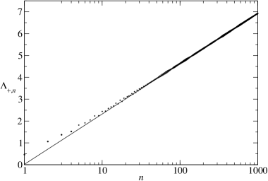
Figure 8: As fig. 5, but for the $\Lambda_{+,n}$ of the Davenport–Heilbronn (DH) function $f_{+}$ as given by (96), up to $n=1000$; e.g., $\Lambda_{+,1}\approx 0.4653858106$, $\Lambda_{+,2}\approx 1.063986745$. Straight line: the GRH-true form $(\log n+C_{5})$ of (97).

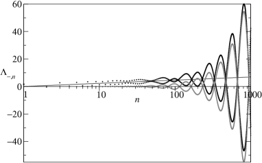
Figure 9: As fig. 8, but for the $\Lambda_{-,n}$ of the DH function $f_{-}$ (vertical scale shrunk); e.g., $\Lambda_{-,1}\approx 1.661697636$, $\Lambda_{-,2}\approx-0.3913729841$ (already $<0$). Straight line: the GRH-true form $(\log n+C_{5})$ as in fig. 8; gray dots: the leading GRH-false form $2\mathop{\rm Re\,}\nolimits F^{\rm odd}_{n}(\rho^{\prime}_{-})$ from (79), (98), with $\rho^{\prime}_{-}\approx 2.30862+8.91836\,{\rm i}$.

These Davenport–Heilbronn (DH) functions $f_{\pm}$ (denoted $f_{1\atop 2}$ in [4], $f(\cdot\,;\tau_{\pm})$ in [7]) obey the functional equation of odd Dirichlet L-functions, namely (75) with the parity $b=1$ and the period $d=5$, up to a ($\pm$) sign: [4][7, § 5]

$$\xi_{\pm}(x)\stackrel{{\scriptstyle\rm def}}{{=}}(\pi/5)^{-x/2}\,\Gamma[{\textstyle{1\over 2}}(1+x)]\,f_{\pm}(x)\equiv\pm\,\xi_{\pm}(1-x).$$ (94)

As in § 3.5, this makes $f_{\pm},\ \xi_{\pm}$ explicit at the positive odd integers:

$$\xi_{\pm}(2m+1)\!\!\! = \!\!\!\mp\frac{2(-1)^{m}}{(2m+1)!!}\,\bigl{[}B_{2m+1}({\textstyle{1\over 5}})+\tau_{\pm}B_{2m+1}({\textstyle{2\over 5}})\bigr{]}\sqrt{\pi}\,(10\,\pi)^{m}\,;$$ (95)

$$e.g.,\quad\xi_{\pm}(1)\!\!\! = \!\!\!\pm{\textstyle{1\over 5}}(3+\tau_{\pm})\sqrt{\pi}\qquad\Bigl{\{}\matrix{\xi_{+}(1)\approx 1.1641757096\cr\xi_{-}(1)\approx 0.1843873182}\Bigr{\}}$$

(we also used $B_{2m+1}(1-a)\equiv-B_{2m+1}(a)$). So, in line with (80) we take

$$\Lambda_{\pm,n}\stackrel{{\scriptstyle\rm def}}{{=}}(-1)^{n}\sum_{m=1}^{n}(-1)^{m}A^{\rm odd}_{mn}\,\log\Biggl{[}\frac{1}{\xi_{\pm}(1)}\xi_{\pm}(2m\!+\!1)\Biggr{]}$$ (96)

as explicit sequences to test our asymptotic criterion for GRH (as (81)–(84) with $\#=$ odd and $d=5$) upon the DH functions $f_{\pm}$ respectively (as instances featuring zeros off the critical line $L$).

Now the numerics break the formal $(\pm)$-symmetry to a surprising extent.

For $\xi_{+}$, the lowest-$T$ zero off the line $L$ is $\rho^{\prime}_{+}\approx 0.808517+85.699348\,{\rm i}$ [31]. Then, for its detection through the sequence $\{\Lambda_{+,n}\}$, our predicted threshold (86) gives $n\approx T^{1+2/t}\approx(85.7)^{7.48}\approx 3\cdot 10^{14}:$ indeed, our low-$n$ data (fig. 8) solely reflect the GRH-true pattern (84) for $d=5$,

$$\Lambda_{+,n}\approx\log n+C_{5},\qquad C_{5}=C+{\textstyle{1\over 2}}\log 5\approx+0.020961845743\,.$$ (97)

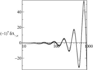
Figure 10: Asymptotics of the deviation (99) from GRH in the case of the DH function $f_{-}$. Black dots: the rectified remainder sequence $(-1)^{n}\delta\Lambda_{-,n}$. Gray dots: the rectified asymptotic form $(-1)^{n}\,2\mathop{\rm Re\,}\nolimits F^{\rm odd}_{n}(\rho^{\prime}_{-})$ from (98). Dashed curve: its large-$(\log n)$ explicit form $2\mathop{\rm Re\,}\nolimits\Bigl{[}\frac{g^{\rm odd}(\rho^{\prime}_{-})}{\rho^{\prime}_{-}(\rho^{\prime}_{-}-1)}n^{\rho^{\prime}_{-}-1/2}\Bigr{]}(\log n)^{-1}$ from (3.5), (82).

Whereas for $\xi_{-}$, the lowest-$T$ zero off $L$ is $\rho^{\prime}_{-}\approx{2.30862+8.91836\,{\rm i}}$ [4]. (Notations therein: $\xi\equiv\tau_{+},\ f_{2}\equiv f_{-}$.) Then, not only is this zero well detached from the next higher one ($\approx 1.94374+18.8994\,{\rm i}$), but above all it gives a detection threshold $n\approx T^{1+2/t}\approx(8.92)^{2.11}\approx 100$, extremely low! Indeed, fig. 9 shows a neat crossover of $\Lambda_{-,n}$ from the GRH-true pattern (97) at low $n$, toward the dominant GRH-false pattern (81) at higher $n$, which is

$$F^{\rm odd}_{n}(\rho^{\prime}_{-})+F^{\rm odd}_{n}({\rho^{\prime}}^{\ast}_{-})\equiv 2\mathop{\rm Re\,}\nolimits F^{\rm odd}_{n}(\rho^{\prime}_{-}).$$ (98)

Even though the form (97) is asymptotically suppressed relatively to (98), in absolute size it remains wholly present in $\Lambda_{-,n}$ which rather follows the straight sum (98)+(97) (fig. 9). Hence to test (98) on $\Lambda_{-,n}$ we first have to subtract (97) from the latter; then just like $\delta\Lambda_{n}$ before (fig. 6), the remainder

$$\delta\Lambda_{-,n}\stackrel{{\scriptstyle\rm def}}{{=}}\Lambda_{-,n}-(\log n+C_{5})$$ (99)

oscillates symmetrically about 0 with period 2, so we rather plot $(-1)^{n}\delta\Lambda_{-,n}$ on fig. 10: we then see a very good fit by $(-1)^{n}\,2\mathop{\rm Re\,}\nolimits F^{\rm odd}_{n}(\rho^{\prime}_{-})$ from (98). In turn, (82) gives the latter an explicit form to first order in ($1/\log n$), which also fits the data well enough (granted that ($1/\log n$) is not so small here).

Thus, numerical data for the sequences $\{\Lambda_{\pm,n}\}$ support our asymptotic alternative in full. We stress that fig. 9 also models how, at some much higher $n$, $\{\Lambda_{n}\}$ itself will blow up if RH (for $\zeta(x)$) is false. Finally, $\{\Lambda_{+,n}\}$ could be a testing ground for any ideas to detect RH-violations earlier with $\{\Lambda_{n}\}$.

4.5 The hitch

We now refocus on the numerical quest for $\{\Lambda_{n}\}$ (the Riemann case), to discuss a major issue. The $(\log n)$-sized values $\Lambda_{n}$ result from alternating summations like (36) over terms growing much faster (exponentially) with $n$: very deep cancellations must then take place, which may explain the sensitivity of $\Lambda_{n}$ (to RH) but also create a computational hurdle for $n\gg 1$, namely a loss of precision growing linearly with $n$. The same issue was seen on $\{\lambda_{n}\}$ empirically [23, fig. 6][18, § 4.2]; here the explicit form of $\Lambda_{n}$ will give us more detailed control over that as well.

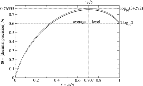
Figure 11: Base decimal precisions needed for the summands of $\Lambda_{n}$ in (36), as estimated by $\log_{10}|A_{nm}\log 2\xi(2m)|$ which is plotted against $m$ in axes rescaled by $1/n$. Dotted curve: the case $n=200$; continuous curve: the $n\to\infty$ limiting form $\varpi=-2\,r\log_{10}r+(1+r)\log_{10}(1+r)-(1-r)\log_{10}(1-r)\quad(r=m/n)$. (Cf. (47) and another, seemingly unrelated, zeta-function calculation [5, § 6.3 & fig. 8].)

For sums $S=\sum s_{m}$ like (36) that come out of order comparable to unity, the slightest end accuracy requires each summand $s_{m}$ to be input with a “base” precision $\approx\log_{10}|s_{m}|$ (working in decimal digits throughout); to which $D$ must be added (uniformly) to aim at $\approx D$ digits of accuracy for $S$.

We can then tune the required precision in (36) for each $m$-value at large given $n$ by using the Stirling formula, to find that $m_{\ast}\approx n/\sqrt{2}$ is where $|s_{m}|$ is largest and the required base precision $\log_{10}|s_{m}|$ culminates, reaching $\log_{10}|A_{nm_{\ast}}\log 2\xi(2m_{\ast})|$ $\sim\log_{10}(3+2\sqrt{2})\,n\approx 0.76555\,n$ digits, see fig. 11 (i.e., $2.5431\,n$ bits, vs $n$ bits for $\lambda_{n}$ [18, § 4.2]). Even then, a crude feed of (36) (or (39), (40)) into a mainstream arbitrary-precision system (Mathematica 10 [37]) suffices to reap the $\Lambda_{n}$-values of § 4.1 effortlessly under $n\approx 20000$. For instance (aiming at $D=13$ digits), the following returns $\Lambda_{10000}$ (but would cater for $n$ of any size in principle, by rewriting the first line only):

In[1]:= n= 10000 ; pr= 7656 + 13 ;
In[2]:= Timing[  Sum[(-1)^m N[ Multinomial[n+m,n-m,2m]/(2m-1)
In[2]:= (Log[ Abs[ BernoulliB[2m]]]-Log[(2m-3)!!]), pr], {m,n}] /(-4)^n
In[2]:= + N[ (1-(-2)^n n!/(2n-1)!!) Log[2 Pi]/2, pr]  ]
Out[2]= {172.295, 8.428662659671506}

coding (39), with a working precision of (7656+13) digits as just argued; all output digits ($16>D=13$) appear to be correct, and CPU time was 172 s. (We used an Intel Xeon E5-2670 0 @ 2.6 GHz processor.) Other samples of computing times we could reach (with some variance between sessions): ca 4 min for $\Lambda_{10000}$, 43 min for $\Lambda_{20000}$ using (40) with targeted precision $D=16$ digits and working precision dynamically adjusted according to fig. 11.

For higher $n$-values, G. Misguich kindly developed a much faster parallel code (available on request), based on the multiple-precision GNU MPFR library [25], and ran it on a 20-core machine still @ 2.6 GHz with 256 Go of memory. He noted that the Bernoulli numbers caused the major part of the workload. He reached CPU times $\approx$ 97 s for $n=20000$, 5.6 h for $n=100000$, 22.7 days for $n=500000$ (without optimizing the precision as in fig. 11; thus $n$ could still be raised, but not so far as to justify the much longer programming and computing times then needed).

Now the true current challenge is to probe $|T|\gtrsim 2.4\cdot 10^{12}$ by (1), hence to reach $n\gtrsim 2\cdot 10^{36}$ (assuming the more favorable estimate (4.2), $10^{60}$ otherwise), which then needs a working precision $\gtrsim 1.6\cdot 10^{36}$ decimal places at times. This need for a huge precision already burdened the original $\lambda_{n}$ but somewhat less and amidst several steeper complexities; now for the $\Lambda_{n}$, the ill-conditioning increased while other difficulties waned. As current status, the $n$-range needed for new tests of RH stays beyond reach for the $\Lambda_{n}$ too.

Still, $\{\Lambda_{n}\}$ has assets to win over $\{\lambda_{n}\}$ in the long run. The $\Lambda_{n}$ are fully explicit; their evaluations are not recursive in $n$, thus very few samples (at high enough $n$, for sure) might suffice to signal that RH is violated somewhere; and the required working precision peaking at $\approx 0.766\,n$ stands as the only stumbling block, but this is a purely logistic barrier, which might be lowered if (36) ever grew better conditioned variants. Already in (39), $\log 2\pi$ needs much less precision ($\propto{\textstyle{1\over 2}}\log_{10}n$) as its coefficient $(2A_{n0})^{-1}\sim-{\textstyle{1\over 2}}\sqrt{\pi n}$ grows negligibly, compared to the ${A_{nm}\log(|B_{2m}|/(2m-3)!!:}$ thus only the latter simpler expressions demand top precision, and mainly for $m\approx n/\sqrt{2}$ (fig. 11); on average over $m$, that demand drops to $(2\log_{10}2)\,n\approx 0.602\ n$ digits ($\equiv 2n$ bits, vs $n$ for $\{\lambda_{n}\}$ [18]). And, to ease the computational burden of the $B_{2m}:$ a) these may be computed just once, to evaluate many $\Lambda_{n}$ in a row; b) only (37) for $2\xi(2m)$ uses $B_{2m}$ but numerically speaking, for large $m$ (41) becomes a much better alternative with its series more and more truncated as $m$ grows. Further improvements of that sort should be pursued in priority to make much higher $n$ accessible. The slow growth of the uncertainty-principle threshold (90) is also an aspect favoring $\{\Lambda_{n}\}$.

Concluding remark and acknowledgments

While other sequences sensitive to RH for large $n$ are known [3][15], not to mention Keiper–Li again, we are unaware of any previous case combining a fully closed form like (36) with a practical sensitivity-threshold of tempered growth $n=O(T^{\nu})$.

We are very grateful to G. Misguich (from our Institute) who wrote and ran a special fast code for numerical calculations reaching $n=500000$ [25]; and to the Referee, for many stimulating comments and suggestions which have helped us to improve this text.

Appendix: Centered variant

We sketch a treatment parallel to the main text for our Li-type sequences using the alternative basepoint $x_{0}={\textstyle{1\over 2}}$, the center for the $\xi$-function [35, §3.4] (and focusing on the Riemann zeros’ case, just for the sake of definiteness).

We recall that the Functional Equation $\xi(1-x)\equiv\xi(x)$ allows us, in place of the mapping $z\mapsto x=(1-z)^{-1}$ within $\xi$ as in (5), to use the double-valued map $y\mapsto x_{\tilde{w}}(y)={\textstyle{1\over 2}}\pm\sqrt{\tilde{w}}\,y^{1/2}/(1-y)$ (parametrized by $\tilde{w}>0$) on the unit disk. That still maps the unit circle ${\{|y|=1\}}$ to the completed critical line $L\cup\{\infty\}$, but now minus its interval $\{|\mathop{\rm Im\,}\nolimits x|<{\textstyle{1\over 2}}\sqrt{\tilde{w}}\}$. As before, we ask all Riemann zeros on $L$ to pull back to ${\{|y|=1\}}$, which imposes $\tilde{w}<\tilde{w}_{0}\stackrel{{\scriptstyle\rm def}}{{=}}4\min_{\rho}|\mathop{\rm Im\,}\nolimits\rho|^{2}\approx 799.1618$. We thus define the parametric sequence $\{\lambda^{0}_{n}(\tilde{w})\}$, for $0<\tilde{w}<\tilde{w}_{0}$, by

$$\log 2\xi\Biggl{(}{\textstyle{1\over 2}}\pm\frac{\sqrt{\tilde{w}}\,y^{1/2}}{1-y}\Biggr{)}\equiv\log 2\xi({\textstyle{1\over 2}})+\sum_{n=1}^{\infty}\frac{\lambda^{0}_{n}(\tilde{w})}{n}\,y^{n}$$ (100)

([35, §3.4] where only the case $\tilde{w}=1$ was detailed, [30]); equivalently,

$$\frac{\lambda^{0}_{n}(\tilde{w})}{n}\equiv\frac{1}{2\pi{\rm i}}\oint\frac{{\rm d}y}{y^{n+1}}\log 2\xi\bigl{(}x_{\tilde{w}}(y)\bigr{)},\qquad n=1,2,\ldots$$ (101)

We now build an explicit variant for this sequence (101), similar to $\{\Lambda_{n}\}$ for $\{\lambda_{n}^{\rm K}\}$. First, the deformations of (101) analogous to those in § 2.1 read as

$$\frac{1}{2\pi{\rm i}}\oint\frac{{\rm d}y}{H_{y_{0}}(y)\cdots H_{y_{n}}(y)}\log 2\xi(x)\qquad(\mbox{here }x\equiv x_{\tilde{w}}(y)),$$ (102)

cf. (25), for which the simplest analytical form we found, mirroring (27), is

$$\frac{1}{2\pi{\rm i}}\oint\frac{2\,{\rm d}r}{(r+1)^{2}}\prod_{m=0}^{n}\frac{r+r_{m}}{r-r_{m}}\,\log 2\xi(x),\qquad r_{m}\stackrel{{\scriptstyle\rm def}}{{=}}\frac{1+y_{m}}{1-y_{m}},$$ (103)

where now $x\equiv x(r)$ with the new variable

$$r\stackrel{{\scriptstyle\rm def}}{{=}}\frac{1+y}{1-y}\equiv\bigl{[}1+(2x-1)^{2}/{\tilde{w}}\bigr{]}^{1/2}\qquad(\mathop{\rm Re\,}\nolimits r>0).$$ (104)

Then with $x_{m}\equiv 2m$ as before (but now including $m=0$), the integral (103) evaluated by the residue theorem yields the result (akin to (36))

$$\Lambda^{0}_{n}(\tilde{w})\stackrel{{\scriptstyle\rm def}}{{=}}\sum_{m=1}^{n}\frac{2}{(r_{m}\!+\!1)^{2}}\frac{\prod\limits_{k=0}^{n}(r_{m}\!+\!r_{k})}{\prod\limits_{k\neq m}(r_{m}\!-\!r_{k})}\log 2\xi(2m),\quad r_{m}\equiv\sqrt{1+(4m\!-\!1)^{2}/{\tilde{w}}}.$$ (105)

These coefficients, while still explicit, are less tractable than the $\Lambda_{n}$ from (36), (32); at the same time their design is more refined in that it captures the Functional Equation (through the $\lambda_{n}^{0}$, and unlike the $\Lambda_{n}$ and $\lambda_{n}$); nevertheless we are yet to see any concrete benefit to using $\{\Lambda^{0}_{n}\}$ over $\{\Lambda_{n}\}$.

Numerical samples (for $\tilde{w}=1$, closest case to $\{\Lambda_{n}\}$; compare with (4.1)):

$$\Lambda^{0}_{1}(1)\approx 0.0881535583,\quad\Lambda^{0}_{2}(1)\approx 0.237357366,\ \ldots,\ \Lambda^{0}_{2000}(1)\approx 6.815307167\,.$$

The corresponding asymptotic alternative for RH analogous to (49)–(3.1) (with $\Delta_{\rho^{\prime}}\Lambda_{n}^{0}$ meaning the contribution to $\Lambda_{n}^{0}$ from the zero $\rho^{\prime}$) reads as

$$\bullet\ \mbox{RH false:}\ \Lambda^{0}_{n}(\tilde{w})\!\!\! \sim \!\!\!\Biggl{\{}\sum_{\mathop{\rm Re\,}\nolimits\rho^{\prime}>1/2}\Delta_{\rho^{\prime}}\Lambda_{n}^{0}(\tilde{w})\Biggr{\}}\pmod{o(n^{\varepsilon})\ \forall\varepsilon>0}$$ (107)

$$\!\!\!\mbox{with }\log|\Delta_{\rho^{\prime}}\Lambda_{n}^{0}(\tilde{w})|\sim(\rho^{\prime}-1/2)\log n,$$

$$\bullet\ \mbox{RH true:}\ \Lambda^{0}_{n}(\tilde{w})\!\!\! \sim \!\!\!\sqrt{\tilde{w}}\,(\log n\!+\!C),\quad C={\textstyle{1\over 2}}(\gamma\!-\!\log\pi\!-\!1)\mbox{ as in (\ref{LRH})}.\qquad$$ (108)

The latter is proved by extending Oesterlé’s method just as with $\Lambda_{n}$; whereas the former needs large-$n$ estimations of the product in (103), but our current ones remain crude compared to the full Stirling formula available for (30); that precludes us from reaching the absolute scales of the $\Delta_{\rho^{\prime}}\Lambda_{n}^{0}(\tilde{w})$ and hence the values of $n$ from which any such terms might become detectable.

Numerically though (all our tests of § 4 admit centered versions), the deviations we observed from the non-centered data (main text) were all slight, especially so for $n\gg 1$, aside from the overall factor $\sqrt{\tilde{w}}$ in (108).

References

- [1] J. Arias de Reyna, Asymptotics of Keiper–Li coefficients, Funct. Approx. Comment. Math. 45 (2011) 7–21.
- [2] R. Ayoub, An Introduction to the Analytic Theory of Numbers, Mathematical Surveys 10, Amer. Math. Soc., Providence, RI (1963).
- [3] L. Báez-Duarte, A sequential Riesz-like criterion for the Riemann Hypothesis, Int. J. Math. Math. Sci. 21 (2005) 3527–3537.
- [4] E.P. Balanzario and J. Sánchez-Ortiz, Zeros of the Davenport–Heilbronn counterexample, Math. Comput. 76 (2007) 2045–2049.
- [5] G. Beliakov and Y. Matiyasevich, Approximation of Riemann’s zeta function by finite Dirichlet series: a multiprecision numerical approach, Exp. Math. 24 (2015) 150–161.
- [6] P. Biane, J. Pitman and M. Yor, Probability laws related to the Jacobi theta and Riemann zeta functions, Bull. Amer. Math. Soc. 38 (2001) 435–465.
- [7] E. Bombieri and A. Ghosh, Around the Davenport–Heilbronn function, Uspekhi Mat. Nauk 66 (2011) 15–66, Russian Math. Surveys 66 (2011) 221–270.
- [8] E. Bombieri and J.C. Lagarias, Complements to Li’s criterion for the Riemann Hypothesis, J. Number Theory 77 (1999) 274–287.
- [9] M.W. Coffey, Toward verification of the Riemann Hypothesis: application of the Li criterion, Math. Phys. Anal. Geom. 8 (2005) 211–255.
- [10] M.W. Coffey, New results concerning power series expansions of the Riemann xi function and the Li/Keiper constants, Proc. R. Soc. Lond. A 464 (2008) 711–731, and refs. therein.
- [11] H. Davenport, Multiplicative Number Theory, 3rd ed. revised by H.L. Montgomery, Graduate Texts in Mathematics 74, Springer, New York (2000), and refs. therein.
- [12] H. Davenport and H. Heilbronn, On the zeros of certain Dirichlet series I, II, J. London Math. Soc. 11 (1936) 181–185, 307–312.
- [13] R.B. Dingle, Asymptotic Expansions: their Derivation and Interpretation, Academic Press, London (1973).
- [14] A. Erdélyi, Asymptotic Expansions, Dover, New York (1956).
- [15] Ph. Flajolet and L. Vepstas, On differences of zeta values, J. Comput. Appl. Math. 220 (2008) 58–73, and refs. therein.
- [16] X. Gourdon, The first zeros of the Riemann Zeta function, and zeros computation at very large height, preprint (Oct. 2004),http://numbers.computation.free.fr/Constants/Miscellaneous/zetazeros1e13-1e24.pdf
- [17] I.S. Gradshteyn and I.M. Ryzhik, Table of Integrals, Series and Products, 5th ed. edited by A. Jeffrey, Academic Press (1994).
- [18] F. Johansson, Rigorous high-precision computation of the Hurwitz zeta function and its derivatives, Numer. Algor. 69 (2015) 253–270.
- [19] J.B. Keiper, Power series expansions of Riemann’s function, Math. Comput. 58 (1992) 765–773.
- [20] J.C. Lagarias, Li coefficients for automorphic -functions, Ann. Inst. Fourier, Grenoble 57 (2007) 1689–1740.
- [21] X.-J. Li, The positivity of a sequence of numbers and the Riemann Hypothesis, J. Number Theory 65 (1997) 325–333.
- [22] K. Maślanka, Li’s criterion for the Riemann hypothesis — numerical approach, Opuscula Math. 24 (2004) 103–114.
- [23] K. Maślanka, Effective method of computing Li’s coefficients and their properties, preprint (2004), arXiv:math.NT/0402168 v5.
- [24] K. Maślanka, Báez-Duarte’s criterion for the Riemann Hypothesis and Rice’s integrals, preprint (2006), arXiv:math/0603713 v2 [math.NT].
- [25] G. Misguich, calculations for , using http://www.mpfr.org/ (private communications, 2017).
- [26] J. Oesterlé, Régions sans zéros de la fonction zêta de Riemann, typescript (2000, revised 2001, uncirculated).
- [27] B. Riemann, Über die Anzahl der Primzahlen unter einer gegebenen Grösse, Monatsb. Preuss. Akad. Wiss. (Nov. 1859) 671–680 [English translation, by R. Baker, Ch. Christenson and H. Orde: Bernhard Riemann: Collected Papers, paper VII, Kendrick Press, Heber City, UT (2004) 135–143].
- [28] W. Rudin, Real and Complex Analysis, McGraw–Hill, New York (1966).
- [29] S.K. Sekatskii, Generalized Bombieri–Lagarias’ theorem and generalized Li’s criterion with its arithmetic interpretation, Ukr. Mat. Zh. 66 (2014) 371–383, Ukr. Math. J. 66 (2014) 415–431; and: Asymptotic of the generalized Li’s sums which non-negativity is equivalent to the Riemann Hypothesis, arXiv:1403.4484 [math.NT] (2014).
- [30] S.K. Sekatskii, Analysis of Voros criterion equivalent to Riemann Hypothesis, Analysis, Geometry and Number Theory 1 (2016) 95–102; arXiv:1407.5758 [math.NT].
- [31] R. Spira, Some zeros of the Titchmarsh counterexample, Math. Comput. 63 (1994) 747–748.
- [32] E.C. Titchmarsh, The Theory of the Riemann Zeta-Function, 2nd ed. revised by D.R. Heath-Brown, Oxford Univ. Press, Oxford (1986).
- [33] A. Voros, A sharpening of Li’s criterion for the Riemann Hypothesis, preprint (Saclay-T04/040 April 2004, unpublished, arXiv: math.NT/0404213 v2), and Sharpenings of Li’s criterion for the Riemann Hypothesis, Math. Phys. Anal. Geom. 9 (2006) 53–63. 333Erratum: our asymptotic statements for in the RH false case have wrong sign.
- [34] A. Voros, Zeta Functions over Zeros of Zeta Functions, Lecture Notes of the Unione Matematica Italiana 8, Springer-Verlag, Berlin (2010).3
- [35] A. Voros, Zeta functions over zeros of Zeta functions and an exponential-asymptotic view of the Riemann Hypothesis, in: Exponential Analysis of Differential Equations and Related Topics (Proceedings, Kyoto, oct. 2013, ed. Y. Takei), RIMS Kôkyûroku Bessatsu B52 (2014) 147–164, arXiv:1403.4558 [math.NT].
- [36] A. Voros, An asymptotic criterion in an explicit sequence, preprint IPhT15/106 (June 2015), HAL archive: cea-01166324, and Simplifications of the Keiper/Li approach to the Riemann Hypothesis, IPhT16/011 (Feb. 2016), arXiv:1602.03292 [math.NT]444Eqs. (35), (40), (51) have typos, fixed in the present work. (unpublished).
- [37] S. Wolfram, Mathematica, 3rd ed., Wolfram Media/Cambridge University Press, New York (1996).