Inflationary Dynamics with a Smooth Slow-Roll to Constant-Roll Era Transition

Abstract

In this paper we investigate the implications of having a varying second slow-roll index on the canonical scalar field inflationary dynamics. We shall be interested in cases that the second slow-roll can take small values and correspondingly large values, for limiting cases of the function that quantifies the variation of the second slow-roll index. As we demonstrate, this can naturally introduce a smooth transition between slow-roll and constant-roll eras. We discuss the theoretical implications of the mechanism we introduce and we use various illustrative examples in order to better understand the new features that the varying second slow-roll index introduces. In the examples we will present, the second slow-roll index has exponential dependence on the scalar field, and in one of these cases, the slow-roll era corresponds to a type of $\alpha$-attractor inflation. Finally, we briefly discuss how the combination of slow-roll and constant-roll may lead to non-Gaussianities in the primordial perturbations.

1 Introduction

Inflation is considered one of the most successful descriptions of the early Universe [1, 2, 3, 4, 5], since it offered consistent remedies to the old Big Bang cosmological description. The terminology inflation actually characterizes a period of acceleration in the early Universe, and this early-time acceleration era can be realized by various theoretical frameworks [6, 7, 8, 9, 10], with the most frequently used being the canonical scalar field description [1, 2]. According to the latest observational data coming from the Planck collaboration [11], the so-called inflaton, which is the canonical scalar field, must follow a slow-roll trajectory in a plateau like potential for large values of the inflaton field. Actually, a recent research stream indicated that these large plateau potentials belong to a class of potentials which all predict the same spectral index of primordial curvature perturbations and the same scalar-to-tensor ratio. These are known as $\alpha$-attractor models [12, 13, 14, 15, 16, 17, 18, 19, 20, 21, 22, 23, 24, 25, 26, 27, 28, 29, 30] and quite well known and also viable models, such as the Starobinsky model [31, 32] and the Higgs model of inflation [33], actually belong to this class of potentials. Hence, the canonical scalar field realization of inflation has quite appealing attributes which mainly are to our opinion, the compatibility with the observations and also the holistic and appealingly simple description of inflation that the $\alpha$-attractor models offer.

However one drawback of the single field inflation models is that these models do not leave any “free space” for future observational data that predict non-Gaussianities in the primordial density perturbations. Actually, the Gaussian property of the primordial modes is an assumption stemming from the fact that the modes are considered uncorrelated (for a review on non-Gaussianities see [34]). Up to date, observations show that the primordial density perturbations have a Gaussian distribution, but the cosmic variance is a considerable limitation for any existing detection method. In the future, if the observations of the Cosmic Microwave Background (CMB) anisotropy and of the galaxy distribution are combined, then it is possible to detect non-Gaussianities in the perturbations. In effect, this will call into question the canonical scalar field and also slow-rolling models of inflation. Also, in conjunction with future observations of non-Gaussianities, the fact that low multipoles are suppressed in the CMB spectrum [11] makes compelling to modify the single scalar field models in order to make them robust against future observations.

One way to allow non-Gaussianities to occur in the predicted spectrum by single scalar field models, is to abandon the slow-roll condition, and a recent important research stream adopted this approach [35, 36, 37, 38, 39, 40, 41, 42, 43, 44, 45, 46, 47]. These models are called constant-roll models [41], or fast-roll models [40], but for the purpose of simplicity in this paper we shall refer to these as “constant-roll” models. These scenarios are quite appealing, since in some cases, viability with observations can be achieved [43], but also non-Gaussianities are predicted in these theories [39, 40]. In addition, for some alternative works on reconstruction of inflationary potentials from the slow-roll indices, see [48, 49].

Due to the phenomenological importance of constant-roll models, but also due to the successes of slow-roll models, in this paper we shall investigate how it is possible to smoothly combine these two eras, in the context of single canonical scalar field theory. Particularly, we shall demonstrate how it is possible to describe a smooth dynamical transition between these two eras. This will be achieved by allowing the second slow-roll index $\eta$ to be a general function of the scalar field, appropriately chosen so that both eras are realized. Obviously the condition $\eta\ll 1$ realizes the slow-roll era, and when $\eta$ becomes of the order $\eta\sim\mathcal{O}(1)$, then the constant-roll era commences. We shall present various models, with the constant-roll era occurring before or after the slow-roll era. The most appealing case generates a slow-roll era which corresponds to the $\alpha$-attractor potentials [12, 13, 14, 15, 16, 17, 18, 19, 20, 21, 22, 23, 24, 25, 26] at leading order. We also support numerically our analytical approach, and as we demonstrate, at least in the context of our models, the constant-roll inflation must occur after the slow-roll era, since in the opposite case, the resulting evolution does not have a unique attractor, and the initial conditions of the scalar field crucially alter the final attractor. This feature however is very model dependent as we shall demonstrate.

Throughout this work we shall assume that the geometric background is a flat Friedmann-Robertson-Walker metric of the form,

$$ds^{2}=-dt^{2}+a(t)^{2}\sum_{i=1,2,3}\left(dx^{i}\right)^{2}\,,$$ (1.1)

where $a(t)$ is the scale factor. Moreover, we assume that the connection is a symmetric, metric compatible and torsion-less affine connection, the Levi-Civita connection.

This paper is organized as follows: In section II we shall present the formalism and the basic features of the dynamical transition mechanism, and we discuss various modifications of single scalar field inflationary dynamics, that this mechanism brings along. In section III we present a first model for which the transition between slow-roll and constant-roll eras is achieved, and we discuss the various features of it. Also we investigate if the resulting solution is an attractor of the cosmological system, both numerically and analytically. Also the slow-roll era is analyzed in some detail, and as we show, the resulting observational indices are identical to the ones corresponding to $\alpha$-attractor models. In section IV we discuss another similar scenario which realizes the constant-roll to slow-roll transition, and the stability of the solution is also investigated in detail.

2 Dynamical Transition Between Constant-Roll Inflation and Slow-Roll Inflation: Formalism and Basic Features

Consider a canonical scalar field in a flat FRW Universe, with action,

$$\mathcal{S}=\sqrt{-g}\left(\frac{R}{2}-\frac{1}{2}\partial_{\mu}\phi\partial^{\mu}\phi-V(\varphi))\right)\,,$$ (2.1)

with $V(\varphi)$ being the canonical scalar field potential. The energy density is equal to,

$$\rho=\frac{1}{2}\dot{\varphi}^{2}+V(\varphi)\,,$$ (2.2)

and also the pressure is,

$$P=\frac{1}{2}\dot{\varphi}^{2}-V(\varphi)\,.$$ (2.3)

Hence, the resulting Friedmann equation is,

$$H^{2}=\frac{1}{3M_{p}^{2}}\rho\,,$$ (2.4)

and we easily find that,

$$\dot{H}=-\frac{1}{2M_{p}^{2}}\dot{\varphi}^{2}\,.$$ (2.5)

Also the canonical scalar field satisfies the Klein-Gordon equation,

$$\ddot{\varphi}+3H\dot{\varphi}+V^{\prime}=0\,,$$ (2.6)

with the prime denoting differentiation with respect to the canonical scalar field $\varphi$.

The inflationary dynamics are quantified in terms of the slow-roll parameters $\epsilon$ and $\eta$, which are the lowest order perturbation parameters in the so-called Hubble slow-roll expansion [50]. These are defined as follows,

$$\epsilon=-\frac{\dot{H}}{H^{2}}\,,\quad\eta=-\frac{\ddot{H}}{2H\dot{H}}\,,$$ (2.7)

in terms of the Hubble rate, and can be written in terms of the canonical scalar field as follows,

$$\epsilon=\frac{\dot{\varphi}^{2}}{2M_{p}^{2}H^{2}}\,,\quad\eta=-\frac{\ddot{\varphi}}{2H\dot{\varphi}}\,.$$ (2.8)

The constant-roll inflation models [40, 41, 43] are based on the fact that the second slow-roll index $\eta$, is not small during the inflationary era, but it is constant, so it satisfies $\eta=-n$, where $n$ is a constant parameter [40]. Essentially, this condition eliminates the slow-roll era, which is based on the assumption that during inflation, the slow-roll indices satisfy $\epsilon,\eta\ll 1$, and the various phenomenological implications of the condition $\eta=-n$, were studied in detail in the literature. In this work we shall assume that the second slow-roll index satisfies the following condition,

$$\eta=-f(\varphi(t))\,,$$ (2.9)

or equivalently,

$$\frac{\ddot{\varphi}}{2H\dot{\varphi}}=f(\varphi(t))\,.$$ (2.10)

The function $f(\varphi(t))$ in both Eqs. (2.9) and (2.10) is assumed to be a smooth and monotonic function of the canonical scalar field $\varphi(t)$, which we shall specify in the following sections. The condition (2.10) is the main assumption we shall make in this paper, and we shall see that the transition from a slow-roll era to a constant-roll era is controlled effectively by the condition (2.10). As we shall demonstrate, in all the cases the transition is smooth.

Our strategy is to find the Hubble rate as a function of the canonical scalar field $H(\varphi)$, by using the Hamilton-Jacobi formalism, by solving the equations of motion. We need to note that, as we discuss also later on, the solution $H(\varphi)$ must be checked numerically and analytically in order to validate if it is the attractor of the cosmological dynamical system, by using various initial conditions. Coming back to the cosmological system, since $\dot{H}=\dot{\varphi}\frac{\mathrm{d}H}{\mathrm{d}\varphi}$ we can write Eq. (2.5) as follows,

$$\dot{\varphi}=-2M_{p}^{2}\frac{\mathrm{d}H}{\mathrm{d}\varphi}\,,$$ (2.11)

so by differentiating Eq. (2.11) with respect to the cosmic time, and by substituting the result in Eq. (2.10), we obtain the following differential equation,

$$\frac{\mathrm{d}^{2}H}{\mathrm{d}\varphi^{2}}=-\frac{1}{2M_{p}^{2}}f(\varphi)H(\varphi)\,.$$ (2.12)

The above differential equation will be the master differential equation in this paper, and it will determine the possible attractors of the cosmological system. The scalar potential $V(\varphi)$ can be expressed in terms of $H(\varphi)$, if we substitute Eq. (2.11) in Eq. (2.4), so we get,

$$V(\varphi)=3M_{p}^{2}H(\varphi)^{2}-2M_{p}^{4}(H^{\prime}(\varphi))^{2}\,.$$ (2.13)

By solving the differential equation (2.12), we can substitute the resulting solution $H(\varphi)$ in Eq. (2.13), and obtain the scalar potential $V(\varphi)$.

However, a solution $H(\varphi)$ may not necessarily be an attractor of the cosmological dynamics, so this should be checked both analytically and numerically. For later convenience we discuss here how to check analytically whether a solution $H_{0}(\varphi)$ is an attractor of the cosmological system. Following [50], we consider the variation of Eq. (2.13), and we obtain the following equation,

$$H_{0}^{\prime}(\varphi)\delta H^{\prime}(\varphi)\simeq\frac{3}{2M_{p}^{2}}H_{0}(\varphi)\delta H(\varphi)\,,$$ (2.14)

which can be solved given $H_{0}(\varphi)$, and it has the solution,

$$\delta H(\varphi)=\delta H(\varphi_{0})e^{\frac{3}{2M_{p}^{2}}\int_{\varphi_{0}}^{\varphi}\frac{H_{0}(\varphi)}{H_{0}(\varphi)}}\,,$$ (2.15)

where $\varphi_{0}$ some initial value of the scalar field. Effectively, for a solution $H_{0}(\varphi)$ of the differential equation (2.12), we can check if the solution is an attractor of the cosmological dynamics, if the linear perturbations (3.11) decay or grow. However, a resulting solution can be considered an attractor if also a numerical analysis reveals an attractor behavior in the phase space $(\dot{\varphi}(t),\varphi(t))$. In all the examples we shall study, we shall use both the analytic and the numerical approach.

In order to have transitions between the slow-roll and constant-roll era, it is conceivable that the function $f(\varphi(t))$ must be chosen in such a way so that during the slow-roll era it satisfies $f(\varphi(t))\simeq 0$, and during the constant-roll era the function $f(\varphi(t)$ must be constant, or a slowly-varying function of the cosmic time. In the following sections we shall present two models for which this qualitative behavior occurs, but in principle there exist a vast number of qualitative behaviors that can be realized, depending the choice of $f(\varphi(t))$. As we already stated earlier, the function $f(\varphi(t))$ must be a monotonic function of the scalar field $\varphi$. Before we proceed to the examples, it is important to derive certain relations that will enable us to validate our findings. One important relation can be found by combining Eqs. (2.6), (2.10), (2.11) and (2.13), and it is,

$$\dot{\varphi}=-\frac{V^{\prime}(\varphi)}{H(\varphi)(f(\varphi)+3)}\,,$$ (2.16)

which in the slow-roll era is approximately equal to,

$$\dot{\varphi}=-\frac{V^{\prime}(\varphi)}{H(\varphi)(3)}\,,$$ (2.17)

Consider that we found a solution $H(\varphi)$ of the differential equation (2.12), then if we find the approximate expression for $H(\varphi)$ during the slow-roll, the expressions (2.16) and (2.17) should coincide in the slow-roll limit. Another useful relation is the $e$-foldings number $N$ as a function of $f(\varphi)$. The $e$-foldings number is defined as follows,

$$N=-\int_{t_{k}}^{t}H(t)\mathrm{d}t=-\int_{\varphi_{k}}^{\varphi}\frac{H}{\dot{\varphi}}\mathrm{d}\varphi\,,$$ (2.18)

where $t_{k}$ is the time instance that the horizon crossing occurs, and $\varphi_{k}$ is the value of the canonical scalar field at the horizon crossing. By substituting Eq. (2.17) in Eq. (2.18), we obtain,

$$N=\frac{1}{M_{p}^{2}}\int_{\varphi}^{\varphi_{k}}\frac{V(f(\varphi)+3)}{3V^{\prime}(\varphi)}\mathrm{d}\varphi\,.$$ (2.19)

During the slow-roll era, the above reduces to the well-known relation,

$$N\simeq\frac{1}{M_{p}^{2}}\int_{\varphi}^{\varphi_{i}}\frac{V(\varphi)}{V^{\prime}(\varphi)}\mathrm{d}\varphi\,.$$ (2.20)

In the next two sections we shall present two models which allow a smooth transition between constant-roll and slow-roll eras, and we shall discuss in some detail the theoretical implications of each model.

3 Model I: From Slow-Rolling $\alpha$-attractors to Constant-Roll

Let us assume that the function $f(\varphi(t))$ appearing in Eq. (2.10) is chosen as follows,

$$f(\varphi(t))=e^{-\lambda\varphi(t)}\,,$$ (3.1)

which is monotonic with respect to the scalar field $\varphi(t)$. We shall choose the parameter $\lambda$ for the needs of this section to be $\lambda=\frac{\sqrt{\frac{2}{3\alpha}}}{M_{p}}$, where $\alpha<1$, but for the moment we shall leave this unspecified, in order to provide a general result. For $\lambda$ chosen as quoted above, the function $f(\varphi(t))$ has a quite interesting behavior, since it allows a slow-roll era when $\frac{\varphi}{M_{p}}\gg 1$, but in the case that $f(\varphi)\sim\mathcal{O}(1)$, the constant-roll inflationary era can be realized. Indeed, for large field values, when $\varphi>M_{p}$, and for $\alpha<1$, the function $f(\varphi(t))$ is approximately zero, since the exponential decays quite fast. In order to have a clear quantitative picture of the physics behind the choice (3.1), let us here quote some numerical examples. In Table 1 we present the values of the function $f(\varphi)$, for various values of the scalar field $\varphi$. As it can be seen, for $\varphi>20M_{p}$, we have $f(\varphi)\ll 1$, so effectively the second slow-roll index satisfies $\eta\ll 1$, and therefore the slow-roll era can be realized and it is actually realized as we evince later on in this section. For $\varphi\simeq 0.1\,M_{p}$, the second slow-roll index is of the order $\eta\simeq\mathcal{O}(1)$, so effectively the constant-roll era begins, and in this case $\frac{\ddot{\varphi}}{2H\dot{\varphi}}\simeq 1$. This scenario of constant-roll was described in [41], and it corresponds to $\alpha=-4$ by using the notation of [41], however $\alpha$ in Ref. [41] appears in $\frac{\ddot{\varphi}}{2H\dot{\varphi}}=-(3+\alpha)$. Interestingly enough, the constant-roll scenario corresponding to $f(\varphi)\simeq 1$ yields quite appealing results, since if the power-spectrum is generated during this era, it can be compatible with the observational data, as it was shown in Ref. [43]. However, we shall not discuss the qualitative features of this model, but we concentrate on the transition between the slow-roll and constant-roll eras and in the general solution of the cosmological equations for the function $f(\varphi)$ being chosen as in Eq. (3.1). In addition, we shall investigate how the slow-roll era can rise through the resulting attractor solution. The details for the constant-roll era, that is, the scalar potential and stability of the attractor solution can be found in Refs. [41, 43].

Table 1: Values of the function $f(\varphi)$ for various values of the scalar field for the model (3.1).

Scalar Field Values	Values of the function $f(\varphi)$
$\varphi\simeq 100M_{p}$	$f(\varphi)\simeq 2.26214\times 10^{-40}$
$\varphi\simeq 50M_{p}$	$f(\varphi)\simeq 1.50404\times 10^{-20}$
$\varphi\simeq 20M_{p}$	$f(\varphi)\simeq 1.17735\times 10^{-8}$
$\varphi\simeq M_{p}$	$f(\varphi)\simeq 0.40137$
$\varphi\simeq 0.1M_{p}$	$f(\varphi)\simeq 0.912756$
$\varphi\simeq 0.01M_{p}$	$f(\varphi)\simeq 0.990913$
$\varphi\simeq 0.0001M_{p}$	$f(\varphi)\simeq 0.999909$
$\varphi\simeq 10^{-7}M_{p}$	$f(\varphi)\simeq 1$

Let us focus on the general case with $f(\varphi)$ being chosen as in Eq. (3.1), so by solving the differential equation (2.12), we obtain the following solution $H(\varphi)$,

$$H(\varphi)=C_{1}\,J_{0}\left(\frac{\left(2\sqrt{\beta}\right)e^{-\frac{1}{2}(\lambda\varphi)}}{\lambda}\right)\,,$$ (3.2)

where $J_{0}(x)$ is the Bessel function of the first kind, $C_{1}$ is an integration constant and $\beta=\frac{1}{2M_{p}^{2}}$. The corresponding scalar potential can easily be found by substituting $H(\varphi)$ from Eq. (3.2) in Eq. (2.13), so the result is,

$$V(\varphi)=3C_{1}^{2}M_{p}^{2}J_{0}\left(\frac{\left(2\sqrt{\beta}\right)e^{-\frac{1}{2}(\lambda\varphi)}}{\lambda}\right)^{2}-2\beta C_{1}^{2}M_{p}^{4}e^{-\lambda\varphi}J_{1}\left(\frac{\left(2\sqrt{\beta}\right)e^{-\frac{1}{2}(\lambda\varphi)}}{\lambda}\right)^{2}\,.$$ (3.3)

At this point we shall make a numerical investigation in order to see whether the solution (3.2) is an attractor of the cosmological equations, independently of the initial conditions. By using the following values of the free parameters (recall that $\beta=\frac{1}{2M_{p}^{2}}$), for reasons that will become clear later on,

$$\lambda=\frac{\sqrt{\frac{2}{3\alpha}}}{M_{p}},\,\,\,\alpha=0.9,\,\,\,C_{1}=1\,,$$ (3.4)

in Fig. 1 we plot the phase space behavior of the solution (3.2), for the initial conditions $\varphi(0)=10^{20.2}$ (red line), $\varphi(0)=10^{20.1}$ (green line), $\varphi(0)=10^{20}$ (blue line).

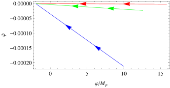
Figure 1: Phase space structure of the solution (3.2), for the initial conditions $\varphi(0)=10^{20.2}$ (red line), $\varphi(0)=10^{20.1}$ (green line), $\varphi(0)=10^{20}$ (blue line).

At it can be seen, all three solutions converge to a unique attractor, so the solution (3.2) is the unique attractor of the cosmological dynamical system. More importantly, the attractor occurs as the scalar field values decrease, and at the same time the velocity of the scalar decreases. Eventually the scalar field settles at some value, when the velocity becomes zero. This can also be verified analytically for the limiting slow-roll case by using Eq. (3.11), but we do this later on. However, we can make a numerical analysis of the solution (3.11), by using $H_{0}(\varphi)$ as in Eq. (3.2). In Fig. 2 we plot the behavior of the exponential in Eq. (3.11), which determines the behavior of the perturbations, for $\varphi$ being chosen in the interval $\varphi=(10^{10},10^{21})$. As it can be seen, for the values of interest, the linear perturbations decay quite rapidly, so this also verifies that the solution (3.2) is actually the solely attractor of the cosmological system.

Figure 2: Stability of linear perturbations for the solution (3.2).

Let us now focus on the slow-roll era, which corresponds to $\varphi>20\,M_{p}$, in which case the arguments of the Bessel functions appearing in Eq. (3.3) are very small. So the potential (3.3) can be approximated as follows,

$$V(\varphi)\simeq-\frac{2\beta^{2}C_{1}^{2}M_{p}^{4}e^{-2\lambda\varphi}}{\lambda^{2}}-\frac{6\beta C_{1}^{2}M_{p}^{2}e^{-\lambda\varphi}}{\lambda^{2}}+3C_{1}^{2}M_{p}^{2}\,.$$ (3.5)

The above potential has very interesting structure since it is quite similar to the Starobinsky model and the $\alpha$-attractor models at leading order. Actually, as we shall evince shortly, the resulting observational indices, that is, the spectral index of the power spectrum of primordial curvature perturbations, and the scalar-to-tensor ratio corresponding to the potential (3.5) are identical to the ones corresponding to the $\alpha$-attractor models. Before proceeding to the calculation of the spectral index and of the scalar-to-tensor ratio, let us validate that the expressions for $\dot{\varphi}$ appearing in Eqs. (2.16) and (2.17) are identical in the slow-roll limit. By substituting $H(\varphi)$ from Eq. (3.2) in Eq. (2.17), we obtain,

$$\dot{\varphi}=-2\sqrt{\beta}C_{1}M_{p}^{2}e^{-\frac{1}{2}\lambda\varphi}J_{1}\left(\frac{2e^{-\frac{1}{2}\lambda\varphi}\sqrt{\beta}}{\lambda}\right)\,,$$ (3.6)

which in the slow-roll limit reads,

$$\dot{\varphi}\simeq-\frac{2\beta C_{1}M_{p}^{2}e^{-\lambda\phi}}{\lambda}\,.$$ (3.7)

Accordingly, by substituting (3.2) in Eq. (2.16), we get,

$$\dot{\varphi}=\frac{2\beta M_{p}^{2}e^{-\lambda\varphi}\,_{0}\tilde{F}_{1}\left(;2;-\frac{e^{-\lambda\varphi}\beta}{\lambda^{2}}\right)\left(3e^{\lambda\varphi}+2\beta M_{p}^{2}\right)}{\lambda\left(\beta-3e^{\lambda\varphi}\right)}\,,$$ (3.8)

where ${}_{0}\tilde{F}_{1}(;z,x)$ is the regularized hypergeometric function. By taking the slow-roll limit, the expression in Eq. (3.9) becomes at leading order,

$$\dot{\varphi}\simeq-\frac{2\beta C_{1}M_{p}^{2}e^{-\lambda\phi}}{\lambda}\,,$$ (3.9)

which is identical with the expression appearing in Eq. (3.7). This result validates that the solution (3.2) yields the correct slow-roll limit for the cosmological system. Also it is worth finding the analytic behavior of the perturbations $\delta H$ appearing in Eq. (3.11) during the slow-roll era. The Hubble rate (3.2) during the slow-roll era can be approximated as,

$$H(\varphi)\simeq 1-\frac{\beta e^{-\lambda\varphi}}{\lambda^{2}}\,,$$ (3.10)

so by substituting in Eq. (3.11), and by integrating with $\varphi$ in the interval $(\varphi_{k},\varphi_{f})$, the resulting expression for the evolution of linear perturbations read,

$$\delta H(\varphi)\simeq\delta H(\varphi_{0})e^{\frac{3}{2M_{p}^{2}}\left(\frac{e^{\lambda\varphi_{f}}}{\beta}-\frac{e^{\lambda\varphi_{k}}}{\beta}\right)}\,,$$ (3.11)

where $\varphi_{f}$ is the value of the scalar field at the time instance that the slow-roll era ends. Since $\varphi_{f}\ll\varphi_{k}$, the exponent of the exponential is negative, and therefore the perturbations $\delta H$ decay in a double exponential way, so quite fast. This result verifies analytically the numerical investigation of Fig. 2, and therefore the solution $H(\varphi)$ is the attractor of the cosmological equations, even during the slow-roll era.

Now let us proceed to the calculation of the observational indices for the scalar potential (3.5). The study of the first slow-roll index will reveal when the slow-roll era actually ends. The Table 1 gives us a first idea on when inflation ends, but only the study of the first slow-roll index will reveal the actual ending of the slow-roll era. However, as we see, the situation is perplexed since the function $f(\varphi)$ is already non-zero at $\varphi_{f}$, hence the approximation starts to collapse. It is therefore possible that the constant-roll takes over before $\varphi_{f}$, so some $e$-folds are done within this constant-roll era. The complete analysis however requires a more detailed numerical approach and it exceeds the purposes of this article so we defer this task to a future work.

During the slow-roll era, the slow-roll indices can be calculated by using the scalar potential, by using the following slow-roll formulas,

$$\epsilon(\varphi)=\frac{M_{p}^{2}}{2}\left(\frac{V^{\prime}(\varphi)}{V(\varphi)}\right)^{2},\,\,\,\eta(\varphi)=M_{p}^{2}\frac{V^{\prime\prime}(\varphi)}{V(\varphi)}\,,$$ (3.12)

so by using the scalar potential (3.3), the first slow-roll index during the slow-roll era,evaluated at the horizon crossing, reads,

$$\epsilon\simeq\frac{2\beta^{2}\lambda^{2}M_{p}^{2}}{\left(\lambda^{2}e^{\lambda\varphi_{k}}-2\beta\right)^{2}}\,,$$ (3.13)

It is vital for the following to calculate the exact value of the scalar field for which $\epsilon\sim\mathcal{O}(1)$, so by solving $\epsilon\sim 1$, we get,

$$\varphi_{f}\simeq\frac{\ln\left(\frac{2\beta+\sqrt{2}\beta\lambda M_{p}}{\lambda^{2}}\right)}{\lambda}\,.$$ (3.14)

In order to have a quantitative idea of the magnitude $\varphi_{f}$, we choose the parameters as in Eq. (3.4) (recall $\beta=\frac{1}{2M_{p}^{2}}$), so $\varphi_{f}$ becomes $\varphi_{f}\simeq 7.45\times 10^{18}$. By looking at Table 1, we can see that for this value, the function $f(\varphi)$ is $f(\varphi)\simeq 0.541$, which is very close to $\mathcal{O}(1)$, but still not one. Hence, it is debatable whether the constant-roll era starts at $\varphi_{f}$. However, we assume here that the slow-roll era stops at $\varphi_{f}$, so after that point the constant-roll era takes over and some $e$-foldings are done during this era. The exit from inflation can be an issue in these constant-roll theories however. In principle the exit from inflation is controlled by the second slow-roll index $\eta$, so when this ceases to be small, exit comes, however a numerical analysis must be performed, and this will be done elsewhere.

During the slow-roll era, the $e$-foldings number $N$ can be expressed in terms of the potential $V(\varphi)$,

$$N\simeq\frac{1}{M_{p}^{2}}\int_{\varphi_{f}}^{\varphi_{i}}\frac{V(\varphi)}{V^{\prime}(\varphi)}\mathrm{d}\varphi\,,$$ (3.15)

where $\varphi_{i}$ is an initial value of the scalar field, which we assume it to be the value at the horizon crossing $\varphi_{k}$. By substituting the potential (3.3) we get at leading order,

$$N\simeq\frac{e^{\lambda\varphi_{k}}-e^{\lambda\varphi_{f}}}{2\beta M_{p}^{2}}\,.$$ (3.16)

By substituting $\varphi_{f}$ from Eq. (3.14) in Eq. (3.16), we obtain $\varphi_{k}$ in terms of $N$,

$$\varphi_{k}\simeq\frac{\log\left(\frac{\beta\left(2\lambda^{2}M_{p}^{2}N-\sqrt{2}\lambda M_{p}+2\right)}{\lambda^{2}}\right)}{\lambda}\,.$$ (3.17)

Hence by substituting (3.17) in Eq. (3.13), the first slow-roll index becomes,

$$\epsilon\simeq\frac{2}{\left(\sqrt{2}-2\lambda M_{p}N\right)^{2}}\,.$$ (3.18)

Accordingly, the second slow-roll index at leading order, evaluated at the horizon crossing, is approximately equal to,

$$\eta\simeq-2\beta M_{p}^{2}e^{-\lambda\varphi_{k}}\,,$$ (3.19)

so by substituting $\varphi_{k}$ from Eq. (3.17), we get,

$$\eta\simeq-\frac{2\lambda^{2}M_{p}^{2}}{2\lambda^{2}M_{p}^{2}N-\sqrt{2}\lambda M_{p}+2}\,.$$ (3.20)

The spectral index of primordial curvature perturbations and the scalar-to-tensor ratio in terms of the slow-roll indices, during the slow-roll era, read,

$$n_{s}\simeq 1-6\epsilon+2\eta,\,\,\,r\simeq 16\epsilon\,,$$ (3.21)

so by substituting Eqs. (3.18) and (3.20) in Eq. (3.21) and by using the $\lambda$ as in Eq. (3.4), we get at leading order for large $N$,

$$n_{s}\simeq 1-\frac{2}{N}-\frac{9}{2N^{2}},\,\,\,r\simeq\frac{12\alpha}{N^{2}}\,.$$ (3.22)

These are identical to the $\alpha$-attractors observational indices, so we are confronted with this interesting scenario of having a slow-roll era which lasts approximately $50-60$ $e$-folds, which is followed immediately by a constant-roll era. Then it is possible that the constant-roll era takes over and controls the dynamics, as this was described in Refs. [40, 41, 43]. Then one could speculate that non-Gaussianities can be generated, since their three-point functions depend on the slow-roll indices. Actually, by using the results of [40], a rough estimate of the parameter $f_{NL}$ for the constant-roll scenario we describe in this paper is $f_{NL}\simeq 7.5$, which can be verified or excluded by future observations. Actually this value is within the current bound $-10<f_{NL}<110$, if $f_{NL}$ is assumed to be momentum independent, which corresponds to local non-Gaussianities. However, one should be cautious with regards to the three-point functions, since the three-point functions are calculated in a conformal time interval, for which the initial time corresponds to an era that the corresponding $f_{k}$ modes are well inside the Hubble radius during the inflationary era. In this paper we approximated the potential during the slow-roll era, so we cannot be sure that if we use these semi-analytic approximations, we shall get accurate results. An accurate approach requires a full analytic treatment, or a detailed numerical treatment, which however exceeds the purposes of this work.

Before closing we need to note that it is possible to construct a variant model of the one appearing in Eq. (3.1), for which the constant-roll era occurs before the slow-roll era. For example, if we choose the function $f(\varphi)$ as follows,

$$f(\varphi)=e^{-\lambda(\varphi-x_{0})}\,,$$ (3.23)

with $x_{0}\simeq M_{p}$. Then, the resulting solution of the differential equation (2.12) is,

$$H(\varphi)=C_{1}J_{0}\left(\frac{2\sqrt{\beta}\sqrt{e^{-\lambda(x_{0}-\varphi)}}}{\lambda}\right)\,.$$ (3.24)

The corresponding scalar potential is,

$$V(\varphi)=3M_{p}^{2}J_{0}\left(\frac{2e^{\frac{1}{2}\lambda(\varphi-x_{0})}\sqrt{\beta}}{\lambda}\right){}^{2}-2\beta M_{p}^{4}e^{\lambda(\varphi-x_{0})}J_{1}\left(\frac{2e^{\frac{1}{2}\lambda(\varphi-x_{0})}\sqrt{\beta}}{\lambda}\right){}^{2}\,.$$ (3.25)

We performed a detailed numerical analysis for the solution (3.24), and the results appear in Fig. (3) in which we plot the phase space evolution corresponding to the solution (3.24). We use the values $x_{0}\simeq M_{p}$, and the rest of the parameters as in Eq. (3.4), with $\beta=\frac{1}{2M_{p}^{2}}$. The red curve corresponds to the initial condition $\varphi(0)=10^{20.2}$ and the blue curve to $\varphi(0)=10^{20}$.

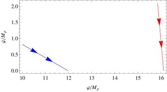
Figure 3: Phase space structure of the solution (3.24). The red curve corresponds to the initial condition $\varphi(0)=10^{20.2}$ and the blue curve to $\varphi(0)=10^{20}$.

As it can be seen in Fig. (3), the solution is very sensitive to initial conditions, and therefore the solution (3.24) is not an attractor of the cosmological dynamics. Hence we refer from going into details for this case. However, the feature we just described, that is, the non-attractor feature that is met when the constant-roll occurs before inflation, is very model dependent.

4 Constant-Roll Before the Slow-Roll Era: A Toy Model

Let us now assume that the function $f(\varphi(t))$ in Eq. (2.10) has the following form,

$$f(\varphi)=3\,e^{-\frac{\lambda\varphi}{M_{p}}}-3\,,$$ (4.1)

where $\lambda$ is a positive number which can be arbitrary. Then, the function $f(\varphi)$ for $\varphi>M_{p}$ is $f(\varphi)\simeq-3$ , and for $\varphi\ll M_{p}$, it approaches zero. Thus in this scenario, the constant-roll era occurs before the slow-roll era, and in this section we examine in brief the qualitative features of this scenario. In Table 2 we present some characteristic values of the function $f(\varphi)$ for various values of the scalar field $\varphi$.

Table 2: Values of the function $f(\varphi)$ for various values of the scalar field for the model (4.1).

Scalar Field Values	Values of the function $f(\varphi)$
$\varphi\simeq 100M_{p}$	$f(\varphi)\simeq-3$
$\varphi\simeq 10M_{p}$	$f(\varphi)\simeq-3$
$\varphi\simeq 5M_{p}$	$f(\varphi)\simeq-2.99986$
$\varphi\simeq M_{p}$	$f(\varphi)\simeq-2.59399$
$\varphi\simeq 0.01M_{p}$	$f(\varphi)\simeq-0.059404$
$\varphi\simeq 10^{-6}M_{p}$	$f(\varphi)\simeq-5.99999\times 10^{-6}$
$\varphi\simeq 10^{-10}M_{p}$	$f(\varphi)\simeq-6\times 10^{-10}$

As it can be seen, for $\varphi>10M_{p}$, the constant-roll era occurs, and for $\varphi\preceq 10^{-6}M_{p}$, the slow-roll era takes over. Hence, for large field values, the constant-roll era occurs, and the cosmological system continuously deforms to the slow-roll era, which takes place for small values of the scalar field. Let us note that the case constant-roll case described by Eq. (4.1) describes the $\alpha=0$ case of Ref. [41], or the $n=-3$ case of Ref. [40], which is called ultra-slow-roll in that work. Naively, one could claim that the evolution is controlled by the dynamics of constant-roll up to the point that the field values become of the order $\varphi\simeq 10^{-6}M_{p}$, however this is not so as we now evince. This could be true if one sees the cosmological equations in their constant-roll limit or slow-roll limit, but if we use the dynamical approach quantified by the function $f(\varphi(t))$, the resulting picture is different. This is due to the fact that the solution of Eq. (2.12) must be the attractor of the cosmological system, and also the correct attractor, that is, the phase space curves must tend to a phase space point for which the velocity of the field is zero, as the scalar field values decrease. Eventually the ideal situation is that the velocity becomes zero at the attractor point, which shows that the field settles at a point as it rolls down to its potential. This is not the case for the model (4.1) as we now evince. The solution of the differential equation (2.12) for the model (4.1) is,

$$H(\varphi)=C_{1}\Gamma\left(1+\frac{\sqrt{6}}{\lambda}\right)J_{\frac{\sqrt{6}}{\lambda}}\left(\frac{\sqrt{6}e^{-\frac{\varphi\lambda}{2M_{p}}}}{\lambda}\right)\,.$$ (4.2)

It can be shown that in the slow-roll limit, the leading order potential is,

$$V(\varphi)\simeq\delta e^{-\frac{\sqrt{6}\varphi}{M_{p}}}\,,$$ (4.3)

where $\delta$ is a constant parameter which is positive but we do not quote it’s analytic form for brevity. The full form of the potential corresponding to the solution (4.3) is found by substituting (4.3) in Eq. (2.13), and we get,

$$V(\varphi)=3C_{1}^{2}M_{p}^{2}\Gamma\left(1+\frac{\sqrt{6}}{\lambda}\right)^{2}J_{\frac{\sqrt{6}}{\lambda}}\left(\frac{\sqrt{6}e^{-\frac{\lambda\varphi}{2M_{p}}}}{\lambda}\right){}^{2}$$ (4.4)

$$-\frac{3}{4}C_{1}^{2}M_{p}^{2}\Gamma\left(1+\frac{\sqrt{6}}{\lambda}\right)^{2}e^{-\frac{\lambda\varphi}{M_{p}}}\left(J_{\frac{\sqrt{6}}{\lambda}-1}\left(\frac{\sqrt{6}e^{-\frac{\lambda\varphi}{2M_{p}}}}{\lambda}\right)-J_{1+\frac{\sqrt{6}}{\lambda}}\left(\frac{\sqrt{6}e^{-\frac{\lambda\varphi}{2M_{p}}}}{\lambda}\right)\right){}^{2}\,.$$

Let us make a numerical investigation in order to validate whether the solution (4.2) is an attractor of the cosmological equations in this case. We use the following values of the free parameters, without loss of generality, $\lambda=0.2$, $C_{1}=1$, and in Fig. 4 we plot the phase space behavior of the solution (4.2), for the initial conditions $\varphi(0)=10^{20.2}$ (red line), $\varphi(0)=10^{20}$ (green line), $\varphi(0)=10^{19.9}$ (blue line).

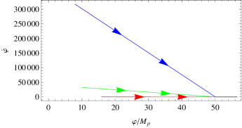
Figure 4: Phase space structure of the solution (4.2), for the initial conditions $\varphi(0)=10^{20.2}$ (red line), $\varphi(0)=10^{20}$ (green line), $\varphi(0)=10^{19.9}$ (blue line).

As it can be seen in Fig. 4, there is an attractor behavior, since all the solutions converge to the same point, however, the attractor occurs in the opposite direction from the desirable one. Indeed, as the field value decreases, the velocity of the scalar field grows, and this is not a desirable feature. So it seems that the solution (4.2) is not an attractor of the cosmological system. In order to further support this argument, we shall investigate the evolution of linear perturbations, as these are given by Eq. (3.11), for the solution (4.2). The results of our analysis appear in Fig. 5, and as it can be seen, the linear perturbations from the solution (4.2) grow very rapidly. Hence, this further supports our argument that the solution (4.2) is not an attractor of the cosmological dynamics for the model (4.1). We need to note here that this non-attractor behavior related to a constant second slow-roll index $\eta$ is a quite well known phenomenon in the literature. Particularly, the ultra-slow-roll solution of Ref. [37], is an inherently non-attractor solution. Another related scenario describing a constant-roll to a slow-roll transition was presented in [38], in which case, the initial constant-roll phase is a dynamically transient phase. In fact, this scenario has the interesting feature of the constant-roll era occurring before the slow-roll era. This behavior leaves space for a possible graceful exit from inflation, when the slow-roll era ends. We hope to also address this behavior in a future work.

Figure 5: Evolution of linear perturbations of the solution (4.2).

Now the question is if the above behavior occurs in all the cases that the slow-roll era occurs after the constant-roll era, at least in the context of the dynamical mechanism we describe in this paper. By observing the two models we presented so far, namely (3.1) and (4.1), the answer is yes. However, this is not true in the general case, unless it is proved by using generic arguments and in a concrete way. For the moment let us note that this feature is model dependent, always in the context of the dynamical approach we used in this paper. For example, the model (4.6) below, leads to attractor behavior, and the constant-roll era occurs before the slow-roll era.

Before closing we would like to note that the mechanism we propose allows for different transition scenarios, and here we give a couple of interesting cases, which will be addressed elsewhere. An interesting and dynamically stable choice for the function $f(\varphi)$ is the following,

$$f(\varphi)=-\frac{1}{\lambda\frac{\varphi}{M_{p}}+\beta}\,,$$ (4.5)

where $\lambda$ is a positive dimensionless constant and the same applies for $\beta$. In the model described by (4.5), for large field values $\varphi>M_{p}$, the function $f(\varphi)$ becomes $f(\varphi)\sim 0$ and for small field values, that is $\varphi\ll M_{p}$, we have $f(\varphi)\simeq-\frac{1}{\beta}$. Therefore, the slow-roll era can be realized for large field values, and the constant-roll for small field values. As it can be shown, the model (4.5) leads to attractor behavior, and the resulting potential during the slow-roll era, is a power-law potential. A variant form of the model (4.5) is the following,

$$f(\varphi)=-\frac{1}{\lambda(\varphi-\varphi_{0})+\beta}\,,$$ (4.6)

in which case the attractor behavior persists, and also constant-roll occurs before the slow-roll era.

Also, with the dynamical mechanism we proposed, it is possible to have transitions between constant-roll eras. For example if we make the following choice,

$$f(\varphi)=-\frac{n}{\gamma\,e^{-\lambda\varphi}+\delta}\,,$$ (4.7)

where $\lambda$ is a positive constant with dimensions $M_{p}^{-1}$, and $\delta>0$, then for large field values, a constant roll era is realized and for small field values, the result is a different constant-roll era. The models (4.6) and (4.7), are quite stable and we aim to study these in some detail elsewhere.

In principle there are more choices for the function $f(\varphi)$, with the most interesting and easy to handle being functions that contain exponentials. Another interesting choice is to use trigonometric functions, so a kind of oscillating behavior would occur, but this study exceeds the purpose of this introductory work.

5 Concluding Remarks

In this work we studied the implications on the dynamics of inflation of a dynamically varying second slow-roll index $\eta$. Particularly we assumed that the second slow-roll index is equal to a function of the canonical scalar field $f(\varphi)$, and we focused on models for which the function, in certain limiting values of the scalar field, becomes either very small or a constant number. The cases that the function is very small correspond to a slow-roll era, and the cases where the function is a constant corresponds to a constant-roll era. This mechanism we studied shows how it is possible to have a transition from a slow-roll to a constant-roll era. As particular examples we studied models which contain exponentials in the function $f(\varphi)$, with the most interesting case leading to a slow-roll era which is characterized by an $\alpha$-attractor evolution, which is followed by a constant-roll evolution. The constant-roll era starts for a value of the scalar field very close to the value for which the first slow-roll index becomes of the order one. We then speculated that it is possible for the cosmological system to follow the constant-roll attractor for some $e$-foldings, in which case certain amount of non-Gaussianities could be generated. The stability of the attractor solution was also checked and we found that the solution is stable and an attractor of the cosmological system. Also we examined the possibility that the constant-roll occurs before the slow-roll era, but the resulting solutions were unstable. As we also commented in the main text, this issue is probably highly model dependent and need to be further studied.

Having a smooth transition from a slow-roll era to a constant-roll era has some attributes but also some drawbacks. For example, the primordial perturbations can be generated during the slow-roll era, and also these do not evolve after the horizon crossing. Then, after the Universe enters the constant-roll era, the non-Gaussianities may be generated. However with this work we did not address in detail this issue, and this has to be done by using the full solution derived by our approach. The analytic treatment however can be tedious, so in a future work we hope to address this at least numerically to some extent. Specifically, if the theory is treated as it behaves in its various limits, it is easy to address all the issues, but if we use the exact analytic solution, the calculations are much more difficult and the various eras cannot be easily distinguished. Therefore only a focused numerical analysis can reveal the true dynamics of our approach. One issue that also needs to be consistently addressed is the graceful exit from inflation. Particularly, usually this exit is identified with the time instance that the first slow-roll index becomes of the order one. However, this indicates that the slow-roll era ends, so if a constant-roll era follows the slow-roll era, the question is then, when does actually inflation ends. This issue is of profound importance since during the constant-roll era, the perturbations generated evolve dynamically, and also the reheating process must start eventually. We hope to address some of these issues elsewhere.

References

- [1] A. D. Linde, Lect. Notes Phys. 738 (2008) 1 [arXiv:0705.0164 [hep-th]].
- [2] D. S. Gorbunov and V. A. Rubakov, “Introduction to the theory of the early universe: Cosmological perturbations and inflationary theory,” Hackensack, USA: World Scientific (2011) 489 p;
- [3] A. Linde, arXiv:1402.0526 [hep-th];
- [4] D. H. Lyth and A. Riotto, Phys. Rept. 314 (1999) 1 [hep-ph/9807278].
- [5] K. Bamba and S. D. Odintsov, Symmetry 7 (2015) 1, 220 [arXiv:1503.00442 [hep-th]]
- [6] S. Nojiri and S. D. Odintsov, eConf C 0602061 (2006) 06 [Int. J. Geom. Meth. Mod. Phys. 4 (2007) 115] [hep-th/0601213].
- [7] S. Capozziello and M. De Laurentis, Phys. Rept. 509 (2011) 167 [arXiv:1108.6266 [gr-qc]].
- [8] V. Faraoni and S. Capozziello, Fundam. Theor. Phys. 170 (2010).
- [9] S. Nojiri and S. D. Odintsov, Phys. Rept. 505 (2011) 59 [arXiv:1011.0544 [gr-qc]].
- [10] T. Clifton, P. G. Ferreira, A. Padilla and C. Skordis, Phys. Rept. 513 (2012) 1 [arXiv:1106.2476 [astro-ph.CO]].
- [11] P. A. R. Ade et al. [Planck Collaboration], Astron. Astrophys. 594 (2016) A20 [arXiv:1502.02114 [astro-ph.CO]].
- [12] R. Kallosh and A. Linde, JCAP 1307 (2013) 002 [arXiv:1306.5220 [hep-th]].
- [13] S. Ferrara, R. Kallosh, A. Linde and M. Porrati, Phys. Rev. D 88 (2013) no.8, 085038 [arXiv:1307.7696 [hep-th]].
- [14] R. Kallosh, A. Linde and D. Roest, JHEP 1311 (2013) 198 [arXiv:1311.0472 [hep-th]].
- [15] M. Galante, R. Kallosh, A. Linde and D. Roest, Phys. Rev. Lett. 114 (2015) no.14, 141302 [arXiv:1412.3797 [hep-th]].
- [16] S. Cecotti and R. Kallosh, JHEP 1405 (2014) 114 [arXiv:1403.2932 [hep-th]].
- [17] J. J. M. Carrasco, R. Kallosh and A. Linde, JHEP 1510 (2015) 147 [arXiv:1506.01708 [hep-th]].
- [18] A. Linde, JCAP 1505 (2015) 003 doi:10.1088/1475-7516/2015/05/003 [arXiv:1504.00663 [hep-th]].
- [19] D. Roest and M. Scalisi, Phys. Rev. D 92 (2015) 043525 doi:10.1103/PhysRevD.92.043525 [arXiv:1503.07909 [hep-th]].
- [20] R. Kallosh, A. Linde and D. Roest, JHEP 1408 (2014) 052 doi:10.1007/JHEP08(2014)052 [arXiv:1405.3646 [hep-th]].
- [21] J. Ellis, D. V. Nanopoulos and K. A. Olive, JCAP 1310 (2013) 009 [arXiv:1307.3537 [hep-th]].
- [22] Y. F. Cai, J. O. Gong and S. Pi, Phys. Lett. B 738 (2014) 20 doi:10.1016/j.physletb.2014.09.009 [arXiv:1404.2560 [hep-th]].
- [23] Z. Yi and Y. Gong, arXiv:1608.05922 [gr-qc].
- [24] R. Kallosh and A. Linde, Phys. Rev. D 91 (2015) 083528 doi:10.1103/PhysRevD.91.083528 [arXiv:1502.07733 [astro-ph.CO]].
- [25] E. V. Linder, Phys. Rev. D 91 (2015) no.12, 123012 doi:10.1103/PhysRevD.91.123012 [arXiv:1505.00815 [astro-ph.CO]].
- [26] E. Elizalde, S. D. Odintsov, E. O. Pozdeeva and S. Y. Vernov, JCAP 1602 (2016) no.02, 025 [arXiv:1509.08817 [gr-qc]].
- [27] R. Kallosh, A. Linde and D. Roest, JHEP 1409 (2014) 062 doi:10.1007/JHEP09(2014)062 [arXiv:1407.4471 [hep-th]].
- [28] S. D. Odintsov and V. K. Oikonomou, Phys. Rev. D 94 (2016) no.12, 124026 doi:10.1103/PhysRevD.94.124026 [arXiv:1612.01126 [gr-qc]].
- [29] S. D. Odintsov and V. K. Oikonomou, arXiv:1611.00738 [gr-qc].
- [30] K. Dimopoulos and C. Owen, arXiv:1703.00305 [gr-qc].
- [31] A. A. Starobinsky, Phys. Lett. B 91 (1980) 99. doi:10.1016/0370-2693(80)90670-X
- [32] J. D. Barrow and S. Cotsakis, Phys. Lett. B 214 (1988) 515. doi:10.1016/0370-2693(88)90110-4
- [33] F. L. Bezrukov and M. Shaposhnikov, Phys. Lett. B 659 (2008) 703 doi:10.1016/j.physletb.2007.11.072 [arXiv:0710.3755 [hep-th]].
- [34] X. Chen, Adv. Astron. 2010 (2010) 638979 doi:10.1155/2010/638979 [arXiv:1002.1416 [astro-ph.CO]].
- [35] S. Inoue and J. Yokoyama, Phys. Lett. B 524 (2002) 15 doi:10.1016/S0370-2693(01)01369-7 [hep-ph/0104083].
- [36] N. C. Tsamis and R. P. Woodard, Phys. Rev. D 69 (2004) 084005 doi:10.1103/PhysRevD.69.084005 [astro-ph/0307463].
- [37] W. H. Kinney, Phys. Rev. D 72 (2005) 023515 doi:10.1103/PhysRevD.72.023515 [gr-qc/0503017].
- [38] K. Tzirakis and W. H. Kinney, Phys. Rev. D 75 (2007) 123510 doi:10.1103/PhysRevD.75.123510 [astro-ph/0701432].
- [39] M. H. Namjoo, H. Firouzjahi and M. Sasaki, Europhys. Lett. 101 (2013) 39001 doi:10.1209/0295-5075/101/39001 [arXiv:1210.3692 [astro-ph.CO]].
- [40] J. Martin, H. Motohashi and T. Suyama, Phys. Rev. D 87 (2013) no.2, 023514 doi:10.1103/PhysRevD.87.023514 [arXiv:1211.0083 [astro-ph.CO]].
- [41] H. Motohashi, A. A. Starobinsky and J. Yokoyama, JCAP 1509 (2015) no.09, 018 doi:10.1088/1475-7516/2015/09/018 [arXiv:1411.5021 [astro-ph.CO]].
- [42] Y. F. Cai, J. O. Gong, D. G. Wang and Z. Wang, JCAP 1610 (2016) no.10, 017 doi:10.1088/1475-7516/2016/10/017 [arXiv:1607.07872 [astro-ph.CO]].
- [43] H. Motohashi and A. A. Starobinsky, arXiv:1702.05847 [astro-ph.CO].
- [44] S. Hirano, T. Kobayashi and S. Yokoyama, Phys. Rev. D 94 (2016) no.10, 103515 doi:10.1103/PhysRevD.94.103515 [arXiv:1604.00141 [astro-ph.CO]].
- [45] L. Anguelova, Nucl. Phys. B 911 (2016) 480 doi:10.1016/j.nuclphysb.2016.08.020 [arXiv:1512.08556 [hep-th]].
- [46] J. L. Cook and L. M. Krauss, JCAP 1603 (2016) no.03, 028 doi:10.1088/1475-7516/2016/03/028 [arXiv:1508.03647 [astro-ph.CO]].
- [47] K. S. Kumar, J. Marto, P. Vargas Moniz and S. Das, JCAP 1604 (2016) no.04, 005 doi:10.1088/1475-7516/2016/04/005 [arXiv:1506.05366 [gr-qc]].
- [48] Q. Gao and Y. Gong, arXiv:1703.02220 [gr-qc].
- [49] J. Lin, Q. Gao and Y. Gong, Mon. Not. Roy. Astron. Soc. 459, no. 4, 4029 (2016) [arXiv:1508.07145 [gr-qc]].
- [50] A. R. Liddle, P. Parsons and J. D. Barrow, Phys. Rev. D 50 (1994) 7222 doi:10.1103/PhysRevD.50.7222 [astro-ph/9408015].