Power-Imbalance Allocation Control of Power Systems-Secondary Frequency Control

Abstract

The traditional secondary frequency control of power systems restores nominal frequency by steering Area Control Errors (ACEs) to zero. Existing methods are a form of integral control with the characteristic that large control gain coefficients introduce an overshoot and small ones result in a slow convergence to a steady state. In order to deal with the large frequency deviation problem, which is the main concern of the power system integrated with a large number of renewable energy, a faster convergence is critical. In this paper, we propose a secondary frequency control method named Power-Imbalance Allocation Control (PIAC) to restore the nominal frequency with a minimized control cost, in which a coordinator estimates the power imbalance and dispatches the control inputs to the controllers after solving an economic power dispatch problem. The power imbalance estimation converges exponentially in PIAC, both overshoots and large frequency deviations are avoided. In addition, when PIAC is implemented in a multi-area controlled network, the controllers of an area are independent of the disturbance of the neighbor areas, which allows an asynchronous control in the multi-area network. A Lyapunov stability analysis shows that PIAC is locally asymptotically stable and simulation results illustrates that it effectively eliminates the drawback of the traditional integral control based methods.

, , ,

1 Introduction

Rapid expansion of the contribution of distributed renewable energy sources has accelerated research efforts in controlling the power grid. In general, frequency control is implemented at three different levels distinguished from fast to slow timescales [29, 17]. In a short time scale, the power grid is stabilized by decentralized droop control, which is called primary control. While successfully balancing the power supply and demand, and synchronizing the power frequency, the primary control induces frequency deviations from the nominal frequency, e.g., 50 or 60 Hz. The secondary frequency control regulates the frequency back to its nominal frequency in a slower time scale than the primary control. On top of the primary and secondary control, the tertiary control is concerned with global economic power dispatch over the networks in a large time scale. Consequently it depends on the energy prices and markets.

The secondary frequency control is the focus of this paper. An interconnected electric power system can be described as a collection of subsystems, each of which is called a control area. The secondary control in a single area is regulated by Automatic Generation Control (AGC), which is driven by Area Control Error (ACE). The ACE of an area is calculated from the local frequency deviations within the area and power transfers between the area and its neighbor areas. The AGC controls the power injections to force the ACE to zero, thus restores the nominal frequency. Due to the availability of a communication network, other secondary frequency control approaches have recently been developed which minimize the control cost on-line [12], e.g., the Distributed Average Integral Method (DAI) [47], the Gather-Broadcast (GB) method [11], economic AGC (EAGC) method [19], and distributed real time power optimal power control method [21]. These methods suffer from a common drawback, namely that they exhibit overshoot for large gain coefficients and slow convergence for small gain coefficients [5, 13, 16]. This is due to the fact that they rely on integral control which is well-known to give rise to the two phenomena mentioned above. Note that the slow convergence speed results in a large frequency deviation which is the main concern of power systems integrated with a large amount of renewable energy.

The presence of fluctuations is expected to increase in the near future, due to weather dependent renewable energy, such as solar and wind energy. These renewable power sources often cause serious frequency fluctuations and deviation from the nominal frequency due to the uncertainty of the weather. This demonstrates the necessity of good secondary frequency control methods whose transient performance is enhanced with respect to the traditional methods. We have recently derived such a method called Power Imbalance Allocation Method (PIAC) in [46], which can eliminate the drawback of the integral control based approach. This paper is the extended version of the conference paper [46] with additional stability analysis and the extension of PIAC to multi-area control.

We consider power systems with lossless transmission lines, which comprise traditional synchronous machines, frequency dependent devices (e.g., power inverters of renewable energy or freqeuncy dependent loads) and passive loads. We assume the system to be equipped with the primary controllers and propose the PIAC method in the framework of Proportional-Integral (PI) control, which first estimates the power imbalance of the system via the measured frequency deviations of the nodes of the synchronous machines and frequency dependent power sources, next dispatches the control inputs of the distributed controllers after solving the economic power dispatch problem. Since the estimated power imbalance converges exponentially at a rate that can be accelerated by increasing the control gain coefficient, the overshoot problem and the large frequency deviation problem is avoided. Hence the drawback of the traditional ACE method is eliminated. Furthermore, the control gain coefficient is independent to the parameters of the power system but only relies on the response time of the control devices. Consequently the transient performance is greatly enhanced by improving the performance of the control devices in PIAC. When implemented in a multi-area power network, PIAC makes the control actions of the areas independent, while the controllers of each area handles the power imbalance of the local area only.

The paper is organized as follows. We introduce the mathematical model of the power system in Section 2. We formulate the problem and discuss the existing approaches in Section 3, then propose the secondary frequency control approach, Power-Imbalance Allocation Control (PIAC), based on estimated power imbalance in Section 4 and analyze its the stability invoking the Lyapunov/LaSalle stability criterion in Section 5. Finally, we evaluate the performance of PIAC by simulations on the IEEE-39 New England test power system in Section 6. Section 7 concludes with remarks.

2 The model

A power system is described by a graph $G=(\mathcal{V},\mathcal{E})$ with nodes $\mathcal{V}$ and edges $\mathcal{E}\subseteq\mathcal{V}\times\mathcal{V}$, where a node represents a bus and edge $(i,j)$ represents the direct transmission line connection between node $i$ and $j$. We consider a power system as a lossless electric network with constant voltage (e.g., transmission grids where the line resistances are neglected) and an adjacency matrix $(\hat{B}_{ij})$ where $\hat{B}_{ij}$ denotes the susceptance between node $i$ and node $j$. The system consists of three types of nodes, synchronous machines, frequency dependent devices and passive loads, the sets of which are denoted by $\mathcal{V}_{M}$, $\mathcal{V}_{F}$ and $\mathcal{V}_{P}$ respectively. Thus $\mathcal{V}=\mathcal{V}_{M}\cup\mathcal{V}_{P}\cup\mathcal{V}_{F}$. The frequency dependent devices are for example frequency dependent loads, inverters of renewable energy, buses equipped with droop controllers. Denote the number of the nodes in $\mathcal{V},\mathcal{V}_{M},\mathcal{V}_{F},\mathcal{V}_{P}$ by $n,~{}n_{M},~{}n_{F}$, and $n_{P}$ respectively, hence $n=n_{M}+n_{F}+n_{P}$. The model is described by the following Differential Algebraic Equations (DAEs), see e.g., [11],

$$\dot{\theta}_{i} =\omega_{i},~{}i\in\mathcal{V}_{M}\cup\mathcal{V}_{F},$$ (1a)

$$M_{i}\dot{\omega}_{i}+D_{i}\omega_{i} =P_{i}-\sum_{j\in\mathcal{V}}{B_{ij}\sin{(\theta_{i}-\theta_{j})}}+u_{i},~{}i\in\mathcal{V}_{M},$$ (1b)

$$D_{i}\omega_{i} =P_{i}-\sum_{j\in\mathcal{V}}{B_{ij}\sin{(\theta_{i}-\theta_{j})}}+u_{i},~{}i\in\mathcal{V}_{F},$$ (1c)

$$0 =P_{i}-\sum_{j\in\mathcal{V}}{B_{ij}\sin{(\theta_{i}-\theta_{j})}},~{}i\in\mathcal{V}_{P},$$ (1d)

where $\theta_{i}$ is the phase angle at node $i$, $\omega_{i}$ is the frequency deviation from the nominal frequency, i.e., $\omega_{i}=\overline{\omega}_{i}-f^{*}$ where $\overline{\omega}_{i}$ is the frequency and $f^{*}=50$ Hz or 60 Hz is the nominal frequency, $M_{i}>0$ denotes the moment of inertia of a synchronous machine, $D_{i}>0$ is the droop control coefficient, $P_{i}$ is the power injection or demand, $B_{ij}=\hat{B}_{ij}V_{i}V_{j}$ is the effective susceptance of line $(i,j)$, $V_{i}$ is the voltage at node $i$, $u_{i}\in[\underline{u}_{i},\overline{u}_{i}]$ is a secondary frequency control input. Note that $u_{i}$ is a constrained input of the secondary frequency control, $\underline{u}_{i}$ and $\overline{u}_{i}$ are its lower and upper bound, respectively. Furthermore, the set of nodes equipped with the secondary controllers is denoted by $\mathcal{V}_{K}\subseteq\mathcal{V}_{M}\cup\mathcal{V}_{F}$ and $u_{i}=0$ for $i\notin\mathcal{V}_{K}$. Here, we have assumed that the nodes that participate in secondary control are equipped with primary controllers. Note that the loads can also be equipped with primary controllers [49]. The dynamics of the voltage and reactive power is not modeled, since they are irrelevant for control of the frequency. More details on decoupling the voltage and frequency control in the power system can be found in [18, 32, 35]. The model with linearized sine functions in (1) is also widely studied to design primary and secondary frequency control laws, e.g., [1, 19, 48]. For the validity of the linearized model with lossless network, we refer to [17, 37].

3 Secondary frequency control of power systems

3.1 Problem formulation

In practice, the frequency deviation should be in a prescribed range in order to avoid damage to the devices in the power system. We assume droop controllers to be installed at some nodes such that $\sum_{i\in\mathcal{V}_{M}\cup\mathcal{V}_{F}}{D_{i}}>0$. When the power supply and demand are time-invariant, the frequencies of all the nodes in $\mathcal{V}_{M}\cup\mathcal{V}_{F}$ synchronize at a state, called synchronous state defined as follows,

$$\theta_{i} =\omega_{syn}t+\theta_{i}^{*},~{}i\in\mathcal{V},$$ (2a)

$$\omega_{i} =\omega_{syn},~{}i\in\mathcal{V}_{M}\cup\mathcal{V}_{F},$$ (2b)

$$\dot{\theta}_{i} =\omega_{syn},~{}i\in\mathcal{V},$$ (2c)

$$\dot{\omega}_{i} =0,~{}i\in\mathcal{V}_{M}\cup\mathcal{V}_{F},$$ (2d)

where $\omega_{syn}$ is the synchronized frequency deviation, and the phase angle differences at the steady state, $\{\theta_{i}^{*}-\theta_{j}^{*},~{}(i,j)\in\mathcal{E}\}$, determine the power flows in the transmission lines. The explicit synchronized frequency deviation $\omega_{syn}$ of the system is obtained by substituting (2) into (1) as

$$\hskip 50.0pt\omega_{syn}=\frac{\sum_{i\in\mathcal{V}}{P_{i}}+\sum_{i\in\mathcal{V}_{K}}{u_{i}}}{\sum_{i\in\mathcal{V}_{M}\cup\mathcal{V}_{F}}{D_{i}}}.$$ (3)

If and only if $\sum_{i\in\mathcal{V}}{P_{i}}+\sum_{i\in\mathcal{V}_{K}}{u_{i}}=0$, the frequency deviation of the steady state is zero, i.e., $\omega_{syn}=0$. This implies that a system with only droop control, i.e., $u_{i}=0,\text{for}~{}i\in\mathcal{V}_{K}$, can never converge to a steady state with $\omega_{syn}=0$ if the power demand and supply is unbalanced such that $\sum_{i\in\mathcal{V}}{P_{i}}\neq 0$. This shows the need for the secondary control. As more renewable power sources are integrated into the power system, the power imbalance $\sum_{i\in\mathcal{V}}{P_{i}}$ may fluctuate severely leading to frequency oscillations. We aim to design an effective method to control $\omega_{syn}$ to zero by solving the following problem, e.g., [12] and [11].

Problem 1.

Compute the inputs {$u_{i},i\in\mathcal{V}_{K}$} of the power system so as to achieve the control objective of a balance of power supply and demand in terms of $\omega_{syn}=0$, or equivalently, $\sum_{i\in\mathcal{V}}{P_{i}}+\sum_{i\in\mathcal{V}_{K}}{u_{i}}=0$.

The following assumption states the basic condition for which a feasible solution of Problem 1 exists.

Assumption 1.

During a small time interval the value of power supply and demand are constant. In addition, for these values there exist control inputs $\{u_{i}\in[\underline{u}_{i},\overline{u}_{i}],i\in\mathcal{V}_{K}\}$, such that $\sum_{i\in\mathcal{V}}{P_{i}}+\sum_{i\in\mathcal{V}_{K}}{u_{i}}=0$.

In a small time interval, the tertiary control, which calculates the operating point stabilized by the secondary control, guarantees the existence of a steady state and its local stability [17, 40]. In addition, the main task of the generators is to provide electricity to the loads and maintain the nominal frequency, so Assumption 1 is realistic.

For different controllers in the system, the control cost might be different for various reasons such as different device maintenance prices. From the global perspective of the entire network, we aim to minimize the secondary frequency control cost which leads to Problem 2.

Problem 2.

Compute the inputs {$u_{i},i\in\mathcal{V}$} of the power system so as to achieve the control objective of minimal control cost, in addition to the control objective of a balance of power supply and demand with $\omega_{syn}=0$.

Corresponding to Problem 2, the following economic power dispatch problem needs to be solved, e.g.,[11, 36].

$$\min_{\{u_{i},i\in\mathcal{V}_{K}\}}\sum_{i\in\mathcal{V}_{K}}J_{i}(u_{i})$$

$$s.t.~{}~{}\sum_{i\in\mathcal{V}}{P_{i}}+\sum_{i\in\mathcal{V}_{K}}{u_{i}}=0.$$

where $J_{i}(u_{i})$ is the control cost of node $i$, which incorporate the cost money and the constraints $u_{i}\in[\underline{u}_{i},\overline{u}_{i}]$. Note that to solve (3.1), the power imbalance $\sum_{i\in\mathcal{V}}{P_{i}}$ should be known and the solution is for the small time interval mentioned in Assumption 1. Here, with respect to the existence of the solution of the economic power dispatch problem, we make the second assumption.

Assumption 2.

The cost functions $J_{i}:\mathbb{R}\rightarrow\mathbb{R},~{}i\in\mathcal{V}_{K}$ are twice continuously differentiable and strictly convex such that $J^{\prime\prime}(u_{i})>0$ where $J^{\prime\prime}(u_{i})$ is the second order derivative of $J(u_{i})$ with respect to $u_{i}$.

Assumption 2 is also realistic because the constraint $u_{i}\in[\underline{u}_{i},\overline{u}_{i}]$ can be incorporated in the objective function $J_{i}(u_{i})$ for $i\in\mathcal{V}_{K}$ in a smooth way.

A necessary condition for solving the economic dispatch problem is [17],

$$\hskip 50.0ptJ^{\prime}_{i}(u_{i})=J^{\prime}_{j}(u_{j})=\lambda,~{}i,j,\in\mathcal{V}_{K}.$$ (5)

where $J^{\prime}_{i}(u_{i})$ is the derivative of $J_{i}(u_{i})$, which is the marginal cost of node $i,i\in\mathcal{V}_{K}$, and $\lambda\in\mathbb{R}$ is the nodal price. At the optimum of (3.1) all the marginal costs of the controllers are equal to the nodal price. The market clearing price $\lambda^{*}$ is obtained as the solution of the equation

$$\hskip 50.0pt0=\sum_{i\in\mathcal{V}}{P_{i}}+\sum_{i\in\mathcal{V}_{K}}{{J^{\prime}}_{i}^{-1}(\lambda^{*})}.$$ (6)

where ${J^{\prime}}_{i}^{-1}(\cdot)$ is the inverse function of $J^{\prime}_{i}(\cdot)$ which exists by Assumption 2. Since in practice the power imbalance is uncertain with respect to the fluctuating power loads, the economic power dispatch problem (3.1) cannot be solved directly.

3.2 A brief review of secondary frequency control

Before embarking on solving Problem 1 and 2, we briefly outline existing secondary frequency control methods and discuss their relevance for finding a solution to Problem 1 and 2.

ACE based AGC[17]: The Area Control Error (ACE) of an area is defined as

$$\hskip 50.0ptACE=B\omega+P_{ex}-P_{ex}^{*},$$ (7)

where $B$ is a positive constant, $\omega$ is the frequency deviation of the area, $P_{ex}$ is the net power export, and $P_{ex}^{*}$ is the nominal value of $P_{ex}$. The adjustment of the power injection of the area is given as follows

$$\hskip 50.0pt\dot{u}=-k\cdot ACE$$

where $k\in(0,\infty)$ is a control gain coefficient. In the traditional Automatic Generation Control (AGC) method, the frequency deviation is measured at a local node and communicated by a coordinator as the ACE to the controllers in the system, which calculate their control inputs according to their participation factors. When the interconnected system is considered as a single area, the AGC has the form [11]

$$\hskip 50.0pt\dot{\lambda}=-k\omega_{i^{*}},~{}i\in\mathcal{V},\quad u_{i}={J^{\prime}}_{i}^{-1}(\lambda),$$ (8)

where $k\in(0,+\infty)$ is a control gain coefficient, $\omega_{i^{*}}$ is the measured frequency deviation at a selected node $i^{*}$. $\lambda$ can be seen as the nodal price which converges to the market clearing price $\lambda^{*}$ as the power supply and demand is balanced. Note that the participation factor is involved in the derivative of the cost function, $J^{\prime}_{i}(u_{i})$. The frequency deviation of the area is not well reflected in (8) since it is measured at only one node. Furthermore, the communication network is not used so efficiently because it only communicates the nodal price $\lambda$ from the coordinator to the controllers.

Gather-Broadcast (GB) Control[11]: In order to well reflect the frequency deviation of the area and use the communication network efficiently, the GB method measures the frequency deviations at all the nodes connected by the communication network. It has the form

$$\hskip 40.0pt\dot{\lambda}=-k\sum_{i\in\mathcal{V}}{C_{i}\omega_{i}},~{}i\in\mathcal{V},\quad u_{i}={J^{\prime}}_{i}^{-1}(\lambda),$$ (9)

where $k\in(0,+\infty)$ is a control gain coefficient and $C_{i}\in[0,1]$ is a set of convex weighting coefficients with $\sum_{i\in\mathcal{V}}{C_{i}}=1$. The ACE in the GB method is actually the weighted average of the frequency deviations. As in the ACE based AGC method (8), a coordinator in the network also broadcasts the nodal price to the controllers and the controllers compute the control inputs according to their own cost functions.

Distributed Averaging Integral control (DAI): Unlike the ACE base AGC method and GB method implemented in a centralized way, DAI is implemented in a distributed way based on the consensus control principle [1]. In the DAI method, there are no coordinators and each controller computes its own nodal price and communicates to its neighbors. A local node in the system calculates its control input according to the local frequency deviation and the nodal prices received from its neighbors. As the state of the interconnected system reaches a new steady state, the nodal prices of all the nodes achieve a consensus at the market clearing price, thus Problem 2 is solved. It has the form [47]

$$\dot{\lambda}_{i}=k_{i}(-\omega_{i}+\sum_{j\in\mathcal{V}}w_{ij}(\lambda_{j}-\lambda_{i})),\quad u_{i}={J^{\prime}}_{i}^{-1}(\lambda_{i}),$$ (10)

where $k_{i}\in(0,+\infty)$ is a gain coefficient for the controller $i$ and $\big{(}w_{ij}\big{)}$ denotes the undirected weighted communication network. When $w_{ij}=0$ for all the lines of the communication network, the DAI control law reduces to a Decentralized Integral (DecI) control law. The DAI control has been widely studied on both the traditional power grids and Micro-Grids, e.g., [31, 33]. Wu et.al. [43] proposed a distributed secondary control method where it is not necessary to know the nominal frequency for all the nodes in $\mathcal{V}_{K}$.

When a steady state exists for the nonlinear system (1), all the approaches above can restore the nominal frequency with an optimized control cost. However, it can be easily observed that the control approaches, e.g., (8) and (9), are in the form of integral control where the control inputs are actually the integral of the frequency deviation. This will be further explained in Section 4. A common drawback of integral control is that the control input suffers from an overshoot problem with a large gain coefficient or slow convergence speed with a small one, which causes extra oscillation or slow convergence of the frequency [5, 13, 16].

The methods that we discussed above, concern controlling the nonlinear system (1) based on passivity methods. However, the linearized version of the evolution equations (1) was also addressed based on primal-dual method in the literature. For example, Li et al. proposed an Economic AGC (EAGC) approach for the multi-area frequency control [19]. In this method each controller exchanges control signals that are used to successfully steer the state of the system to a steady state with optimized dispatch, by a partial primal-dual gradient algorithm [7]. Unfortunately, transient performance was not considered in the method. A potentially very promising method to the control of the linear system was recently proposed by Zhao et al. In [48] a novel framework for primary and secondary control, which is called Unified Control (UC), was developed. The advantage of UC is that it automatically takes care of the congestions that may occur in the transmission lines. Numerical simulations results show that the UC can effectively reduce the harmful large transient oscillations in the frequency. However, so far a theoretical analysis on how the UC improves the transient performance is lacking. Other recently reported study are by Liu et al. in [21] and by Z. Wang et al. in [39]. These methods optimize both control costs and manages power flow congestion using the principle of consensus control, but cannot prevent large frequency deviations at short times. For more details of distributed frequency control, we refer to the survey paper [25].

Finally, we mention here control methods whose underlying principle is neither based on integral control nor on primal-dual method. The optimal load-frequency control framework by Liu et al., described in [20], is an example of such a method. The goal is still to optimize the control costs and frequency deviation, but rephrasing it as a finite horizon optimization problem. This can only be solved when the loads are precisely known within the selected time horizon. Obviously, this will require very precise forecasting of the loads. A more robust approach based on the concept of the Active Disturbance Rejection Control (ADRC) [14], was pursued by Dong et al. [9]. The method is robust against model uncertainties, parameter variations and large perturbations which was employed to construct a decentralized load frequency approach for interconnected systems. However, the decentralized control employed in this method prevents a solution to Problem 2.

As more renewable power sources are integrated into the power system, the fluctuations in the power supply become faster and larger. There is a need to design a control law that has a good transient performance without the overshoot problem and with a fast convergence speed. The traditional method to eliminate the overshoot is to calculate the control gain coefficients by analyzing the eigenvalue of the linearized systems [42, 41]. However, the improvement of the transient performance obtained by the eigenvalue analysis is still poor because of the dependence of the eigenvalues on the control law structure, and the large scale, complex topology and heterogeneous power generation and loads of the power system.

Based on the framework of PI control this paper aims to design a secondary frequency control method that remedies the drawbacks mentioned above of the existing methods. To this end, we consider the following problem concerning the transient performance of the power system (1) after a disturbance.

Problem 3.

For the power system (1) with primary and secondary controllers, design a secondary frequency control law for $\{u_{i},~{}i\in\mathcal{V}_{K}\}$ so as to eliminate the extra oscillation of the frequency caused by the overshoots of the control inputs, thus improve the transient performance of the system after a disturbance through an accelerated convergence of the control inputs.

To address Problem 3, various control laws have been proposed for the frequency control of power systems, e.g., the sliding mode based control laws [38, 23] and $\mathcal{H}_{2}/\mathcal{H}_{\infty}$ control based control laws [6, Chapter 5] and [28] et al, which are able to shorten the transient phase while avoiding the overshoots and large frequency deviations. However, they focus on the linearized system and did not consider the economic power dispatch problem (3.1) at the steady state.

4 Power Imbalance Allocation Control

In this section, we introcuce the Power-Imbalance Allocation Control (PIAC) method to solve Problem 1-3.

The communication network is necessary for solving Problem 2, for which we make the following assumption.

Assumption 3.

All the buses in $\mathcal{V}_{M}\cup\mathcal{V}_{F}$ can communicate with a coordinator at a central location via a communication network. The frequency deviations $\omega_{i},~{}i\in\mathcal{V}_{M}\cup\mathcal{V}_{F}$, can be measured and subsequently communicated to the coordinator. For ${i\in\mathcal{V}_{K}}$, the control input $u_{i}$ can be computed by the coordinator and dispatched to the controller at node $i$ via the communication network.

In Assumption 3, the local nodes need to provide the coordinator the local frequency deviation which are the differences between the measured frequencies by meters and the nominal frequency. We remark that there usually are time-delays in the measurement and communications which are neglected in this paper.

In the following, we first define an abstract frequency deviation of the power system, for which we design a control law to eliminate the overshoot of the control input, then introduce the PIAC method firstly control the power system controlled as a single area and followed by a multi-area approach in subsection (4.1) and (4.2) respectively.

Definition 1.

For the power system (1), define an abstract frequency deviation $\omega_{s}$ such that

$$~{}~{}~{}~{}~{}~{}~{}~{}~{}~{}~{}~{}~{}~{}M_{s}\dot{\omega}_{s}=P_{s}-D_{s}\omega_{s}+u_{s},$$ (11)

where $M_{s}=\sum_{i\in\mathcal{V}_{M}}{M_{i}}$, $P_{s}=\sum_{i\in\mathcal{V}}{P_{i}}$, $D_{s}=\sum_{i\in\mathcal{V}}{D_{i}}$, and $u_{s}=\sum_{i\in\mathcal{V}_{K}}u_{i}$.

Note that $\omega_{s}(t)$ is a virtual global frequency deviation, which neither equals to $\omega_{i}(t)$ nor $\omega_{syn}(t)$ in general. However, if the power loads (or generation) $P_{i}$ change slowly and the frequencies $\{\omega_{i},~{}i\in\mathcal{V}_{M}\cup\mathcal{V}_{F}\}$ synchronize quickly, the differences between $\omega_{i}(t)$ and $\omega_{s}(t)$ are negligible, i.e., $\omega_{i}(t)=\omega_{s}(t)$, by summing all the equations of (1), (11) is derived.

At the steady state of (11), we have $\omega_{s}^{*}=(P_{s}+u_{s})/D_{s}$ which leads to $\omega_{s}^{*}=\omega_{syn}^{*}$ by (3). Then the objective of the secondary frequency control that restores the nominal frequency of the system (1) is equivalent to controlling $\omega_{s}$ of (11) to zero, i.e., $\lim_{t\rightarrow\infty}{\omega_{s}(t)=0}.$

Since the frequencies $\{\omega_{i},~{}i\in\mathcal{V}_{M}\cup\mathcal{V}_{F}\}$ of system (1) with primary controllers synchronize quickly, the extra oscillations of $\omega_{i}$ are actually introduced by the overshoot of the total amount of control inputs $u_{s}$ in the traditional control approach (8). This is because it is in the form of integral control. It will be explained in an extreme case where system (1) is well controlled by primary controllers such that $\omega_{i}=\omega_{s}$ for all $i\in\mathcal{V}$. It can be obtained easily for (8) by substituting $\omega_{i}$ by $\omega_{s}$ that the total amount of control inputs, $u_{s}$, is calculated as follows,

$$\dot{\lambda}_{s}=\omega_{s},$$ (12a)

$$u_{s}=-k\lambda_{s},$$ (12b)

which is in the form of integral control. Note that (12) can also be obtained similarly for the GB method (9) and for the DAI method (10) with a special setting of control gain coefficients $k_{i}$ and communication weight $w_{ij}$ e.g., $\{k_{i},~{}i\in\mathcal{V}_{k}\}$ are all identical and $w_{ij}$ forms a Laplacian matrix, $L=(w_{ij})$, such that $\sum_{i=1}^{n_{K}}{w_{ij}}=0$ for all $j=1,\cdots,n_{K}$( $n_{K}$ is the number of nodes in $\mathcal{V}_{K}$).

In order to accelerate the convergence of the frequency to its nominal value without introducing extra oscillations, the overshoot of $u_{s}$ should be avoided. Similar to the PI cruise control of a car [3], for $\omega_{s}$ in (11), we introduce the following control law,

$$\dot{\eta}_{s}=D_{s}\omega_{s},$$ (13a)

$$u_{s}=-kM_{s}\omega_{s}-k\eta_{s},$$ (13b)

where $k\in(0,+\infty)$ is a parameter to be chosen by engineers. Details on the setting of this parameter will be further discussed after introducing the PIAC method in this section. From (13) and (11), we obtain

$$~{}~{}~{}~{}~{}~{}~{}~{}~{}~{}~{}~{}~{}~{}~{}~{}~{}~{}~{}~{}~{}\dot{u}_{s}(t)=-k(P_{s}+u_{s}(t)),$$ (14)

which indicates that $u_{s}$ is an estimate of $-P_{s}$ and converges to the power imbalance $-P_{s}$ exponentially. Hence, the overshoot of $u_{s}$ is eliminated. With the value of $u_{s}$ obtained from (13), the control input $u_{i}$ for node $i\in\mathcal{V}_{K}$ is computed by solving the following economic power dispatch problem,

$$\min_{\{u_{i}\in\mathbb{R},i\in\mathcal{V}_{K}\}}\sum_{i\in\mathcal{V}_{K}}J_{i}(u_{i}),$$

$$s.t.~{}~{}-u_{s}(t)+\sum_{i\in\mathcal{V}_{K}}{u_{i}}(t)=0.$$

However, $u_{s}$ cannot be calculated as in (13) since $\omega_{s}$ is a virtual frequency deviation which cannot be measured in practice. In the following, we introduce the PIAC method where $u_{s}$ also converges to $-P_{s}$ exponentially as in (14).

4.1 Single-area implementation of PIAC

We consider the power system controlled as a single area without any power export (or import). The PIAC method is defined as follows.

Definition 2 (PIAC).

Consider the power system described by (1) with assumption (1-3), the PIAC control law is defined as the dynamic controller,

$$\dot{\eta}(t) =\sum_{i\in\mathcal{V}_{M}\cup\mathcal{V}_{F}}D_{i}\omega_{i}(t),$$ (16a)

$$u_{s}(t) =-k\Big{(}\eta(t)+\sum_{j\in\mathcal{V}_{M}}{M_{j}\omega_{j}(t)}\Big{)},$$ (16b)

$$0 =-u_{s}(t)+\sum_{i\in\mathcal{V}_{K}}{{J^{\prime}}_{i}^{-1}(\lambda(t))},$$ (16c)

$$u_{i}(t) ={J^{\prime}}_{i}^{-1}(\lambda(t)),~{}i\in\mathcal{V}_{K},$$ (16d)

where $k\in(0,\infty)$ is a parameter of the control law, $\eta$ is a state variable introduced for the integral term as $\eta_{s}$ in (13a), and $\lambda$ is an algebraic variable for solving the optimization problem (4), which is a function of time.

For the special case with quadratic cost function $J_{i}(u_{i})=\frac{1}{2}\alpha_{i}u_{i}^{2}$ for node $i$, the control law becomes

$$\dot{\eta} =\sum_{i\in\mathcal{V}_{M}\cup\mathcal{V}_{F}}{D_{i}\omega_{i}},$$

$$u_{s} =-k(\sum_{i\in\mathcal{V}_{M}}{M_{i}\omega_{i}+\eta_{s}}),$$

$$u_{i} =\frac{\alpha_{s}}{\alpha_{i}}u_{s},~{}i\in\mathcal{V}_{K},$$

$$\frac{1}{\alpha_{s}} =\sum_{i\in\mathcal{V}_{K}}\frac{1}{\alpha_{i}},$$

where $\alpha_{i}\in\mathbb{R}$ is the control price of node $i$.

PIAC is based on the design principle of coordination. The local nodes in $\mathcal{V}_{M}\cup\mathcal{V}_{F}$ send the measured frequency deviations to the coordinator. The coordinator computes the control inputs $\{u_{i},i\in\mathcal{V}_{K}\}$ or marginal cost $\lambda$ using the local measurements and sends them to all local controllers of the nodes indexed by $\mathcal{V}_{K}$. The procedure is similar to the GB method which gathers the locally measured frequency deviation from the nodes and broadcasts the nodal price to the controllers. The control procedure and properties of PIAC are summarized in the following procedure and theorem respectively.

Procedure 1.

If the assumptions 1-3 hold, then the secondary frequency control approach of the power system (1), PIAC, is implemented as follows.

1. Collect the measured frequency deviations

   $$\{\omega_{i},~{}i\in\mathcal{V}_{M}\cup\mathcal{V}_{F}\},$$

2. Calculate the total amount $u_{s}(t)$ of control inputs by (16b),

3. Solve the optimization problem (4) by (16c,16d),

4. Allocate the power compensation $\{u_{i},~{}i\in\mathcal{V}_{K}\}$ to the controllers.

Theorem 1.

Consider the power system (1) and the PIAC control law, the controller has the following properties,

1. at any time, $t\in T$, $u_{s}(t)$ satisfies (14). Thus it is an estimate of the power imbalance $-P_{s}$;

2. at any time, $t\in T$, the input values $\{u_{i}(t),i\in\mathcal{V}_{K}\}$ are computed by solving the optimization problem (4). So the total amount of control inputs, $u_{s}(t)$, are dispatched to the local nodes of $\mathcal{V}_{K}$ economically;

3. at the steady state, $\omega_{i}^{*}=0$ for all $i\in\mathcal{V}_{M}\cup\mathcal{V}_{F}$ and the power-imbalance $P_{s}$ is optimally compensated by the local controllers. Hence both Problem 1 and Problem 2 are solved;

4. because

   $$u_{s}(t)=-k\sum_{i\in\mathcal{V}_{M}}{M_{i}\omega_{i}}(t)-k\int_{0}^{t}{\sum_{j\in\mathcal{V}_{M}\cup\mathcal{V}_{F}}D_{j}\omega_{j}(\tau)d\tau},$$

   the PIAC control law is of proportional-integral type.

Proof: (a). From (1) it follows,

$$\sum_{i\in\mathcal{V}_{M}}M_{i}\dot{\omega}_{i}=\sum_{i\in\mathcal{V}}P_{i}-\sum_{i\in\mathcal{V}_{M}\cup\mathcal{V}_{F}}{D_{i}\omega_{i}}+\sum_{i\in\mathcal{V}}{u_{i}}.$$ (18)

It follows from (16a,16b) that,

$$\dot{u}_{s}(t) =-k\Big{(}\sum_{i\in\mathcal{V}_{M}\cup\mathcal{V}_{F}}D_{i}\omega_{i}(t)+\sum_{j\in\mathcal{V}_{M}}M_{j}\dot{\omega}_{i}(t)\Big{)}$$

by (18),

$$=-k\Big{(}\sum_{i\in\mathcal{V}_{K}}{u_{i}(t)}+\sum_{j\in\mathcal{V}}{P_{i}}\Big{)}$$

by (16d),

$$=-k\Big{(}\sum_{i\in\mathcal{V}_{K}}{{J^{\prime}}_{i}^{-1}(\lambda)}+\sum_{j\in\mathcal{V}}{P_{i}}\Big{)}$$

by (16c),

$$=-k\Big{(}u_{s}(t)+P_{s}\Big{)},$$

Thus (14) is obtained which indicates that $u_{s}(t)$ is an estimate of $-P_{s}$ with $k\in(0,\infty)$, i.e., $u_{s}(t)$ converges to $-P_{s}$ exponentially with a speed determined by the control gain coefficient $k$.

(b). According to the definition of the PIAC control law that at any time, $t\in T$,

$$~{}~{}~{}~{}~{}~{}~{}~{}~{}~{}J^{\prime}_{i}(u_{i}(t))=J^{\prime}_{j}(u_{j}(t))=\lambda(t),~{}\forall~{}i,j\in\mathcal{V}_{K}.$$

Thus the necessary condition (5) for economic dispatch of $u_{s}(t)$ to all the local nodes is satisfied and at any time $t\in T$, the control inputs $\{u_{i},~{}i\in\mathcal{V}_{K}\}$ solve the optimization problem (4). Hence, $\{u_{i}(t),i\in\mathcal{V}\}$ achieve the minimal cost.

(c). It follows from (14) that $u^{*}_{s}=-\sum_{i\in\mathcal{V}}P_{i}$ at the steady state, which yields $\omega_{syn}=0$ by (3). Thus $\omega^{*}_{i}=0$ for all $i\in\mathcal{V}_{M}\cup\mathcal{V}_{F}$ by (2), Problem 1 is solved. It follows from (b) that the control inputs $\{u_{i},i\in\mathcal{V}\}$ achieve minimal cost at the steady state. So the optimization problem (3.1) is solved at the steady state. Hence, Problem 2 is solved.

(d). This follows directly from the definition of the PIAC control law. $\Box$

Note that in Theorem 1(c), we have assumed that the steady state exists which will be further described in Assumption 4 in Section 5.

In order to clearly illustrate how PIAC improves the transient performance of the system, with the abstract frequency deviation $\omega_{s}$ and control inputs $u_{s}$, we decompose the dynamic process into three sub-processes,

1. the convergence process of $u_{s}$ to $-P_{s}$ as in (14) with a speed determined by $k$.

2. the convergence process of $\omega_{s}$ to zero as in (11) with a speed determined by $u_{s}$ and $D_{s}$.

3. and the synchronization process of $\{\omega_{i},~{}i\in\mathcal{V}_{M}\cup\mathcal{V}_{F}\}$ to $\omega_{s}$ described by (1) and with the synchronization speed mainly determined by $\{D_{i},~{}i\in\mathcal{V}_{M}\cup\mathcal{V}_{F}\}$.

The transient performance of the power system can be improved by tuning the corresponding control gain coefficients for the sub-processes. PIAC focuses on the first two sub-processes only in which the transient behaviors of $u_{s}$ and $\omega_{s}$ can be improved by increasing the parameter $k$, and the primary control focuses on the synchronization of $\{\omega_{i},~{}i\in\mathcal{V}_{M}\cup\mathcal{V}_{F}\}$ which can be improved by tuning the coefficient $\{D_{i},~{}i\in\mathcal{V}_{M}\cup\mathcal{V}_{F}\}$ as in [12, 26]. As $u_{s}$ converges to $-P_{s}$ exponentially, the control inputs $\{u_{i},~{}i\in\mathcal{V}_{K}\}$ in (16d) also converge to the desired optimal values in an exponential way without any overshoots and their convergence speed increase with a large $k$. Thus the extra oscillation caused by the overshoot of $u_{s}$ is avoided and Problem 3 is solved by PIAC.

With the process decomposition, the improvement in the transient performance by the UC control law [48] can be explained, and the control gain coefficients of the primal-dual based control laws, e.g.,[39] without triggered constraints of line flows, which also estimate the power disturbance, can be tuned to improve the transient performance.

In the following, we introduce the properties of PIAC in the implementation for the power system controlled as a single area.

On the communications in PIAC, note that the communicated data include dynamic data and static data. The dynamic data are the frequency deviations $\{\omega_{i},~{}i\in\mathcal{V}_{M}\cup\mathcal{V}_{F}\}$ and the control inputs $\{u_{i}~{}i\in\mathcal{V}_{K}\}$, both should be communicated frequently. The static data are the moment inertia $\{M_{i},~{}i\in\mathcal{V}_{i}\}$, the droop control coefficients $\{D_{i},~{}i\in\mathcal{V}_{M}\cup\mathcal{V}_{F}\}$ and the cost functions $\{J_{i}(u_{i}),i\in\mathcal{V}_{K}\}$, which are constant in a short time as in Assumption 1 and are not necessary to communicate as frequently as the dynamic data.

In the computing of the control inputs $\{u_{i},~{}i\in\mathcal{V}_{K}\}$, solving the optimization problem (4) is equivalent to solving the equations (16c) and (16d). So the computation includes calculating the integral of frequency deviation in (16a) and solving the algebraic equation (16c,16d). For quadratic cost functions $J_{i}(u_{i})=\frac{1}{2}\alpha_{i}u_{i}^{2}$, the computation requires approximately $4n_{M}+n_{F}$ arithmetic operations that are $\times$, +, - etc. For nonlinear cost functions, an iteration method is used to solve the one dimension nonlinear algebraic equation (16c) for $\lambda$, which needs more computing than for the quadratic cost functions.

Remark 1.

PIAC is a centralized control where the communications and computations increase as the scale of the power systems increases. In a large-scale power system, a large number of devices communicate to the coordinator simultaneously. In that case, the time-delay due to the communications and computing is not negligible, in such a situation further investgation for the transient performance and stability of the nonlinear system is needed.

On the dynamics of $u_{s}$, it can be observed from (14) that $u_{s}$ converges exponentially with a speed that can be accelerated by increasing the control gain coefficient $k$ which does not depend on any parameters of the power system and the cost functions. Hence, when the dynamics of the voltages are considered which does not influence the dynamics of $u_{s}$ in (14), the power supply and demand can also be balanced.

On the control gain coefficient $k$, we remark that it does neither depend on the parameters of the system nor on the economic power dispatch problem, and can be set very large from the perspective of theoretical analysis. However, it relies on how sensitive the control devices are to the fluctuation of power imbalance. In this case, it can be tuned according to the response time of the control devices and the desired range of the frequency deviation. The control actuators of traditional hydraulic and steam turbines are their governor systems. For details of the model of the governor system and its response time, we refer to [18, chapter 9,11].

By Assumption 3, the PIAC method requires that all the nodes in $\mathcal{V}_{M}\cup\mathcal{V}_{F}$ can communicate with the coordinator. However, our initial numerical experiments show that PIAC can still restore the nominal frequency even without all the frequency deviation collected, where the estimated power imbalance converges to the actual power imbalance although not exponentially. This is because PIAC includes the integral control which drives the synchronized frequency deviation to zero.

Remark 2.

In practice, the state of the power system is never at a true equilibrium state, because of the fluctuating of the power imbalance caused by the power loads. Furthermore, the fluctuations becomes even more serious when a large amount of renewable power sources are integrated into the power system. In this case, it is more practical to model the power imbalance as a time-varying function. For the power system with time-varying power imbalance, analysis and numerical simulations show that PIAC is also able to effectively control the synchronized frequency to any desired range by increasing the control gain coefficient $k$ [45].

4.2 Multi-area implementation of PIAC

When a power system is partitioned into several control areas, each area has either an export or an import of power. After a disturbance occurred, the power export or the power import of an area must be restored to the nominal value calculated by tertiary control. In this subsection, we introduce the implementation of PIAC for multi-area control where each area has power export (or import).

Denote the set of the nodes in the area $A_{r}$ by $\mathcal{V}_{A_{r}}$, the set of the boundary lines between area $A_{r}$ and all the other areas by $\mathcal{E}_{A_{r}}$. Denote $\mathcal{V}_{M_{r}}=\mathcal{V}_{M}\cap\mathcal{V}_{A_{r}}$, $\mathcal{V}_{F_{r}}=\mathcal{V}_{F}\cap\mathcal{V}_{A_{r}}$ and $\mathcal{V}_{K_{r}}=\mathcal{V}_{K}\cap\mathcal{V}_{A_{r}}$. The multi-area control of PIAC in the area $A_{r}$ is defined as follows.

Definition 3.

Consider the power system (1) controlled as several areas with Assumption (1-3), the multi-area implementation of PIAC for area $A_{r}$ is defined as the dynamic controllers,

$$\dot{\eta}_{r}(t) =\sum_{i\in\mathcal{V}_{M_{r}}\cup\mathcal{V}_{F_{r}}}D_{i}\omega_{i}(t)+P_{ex}(t)-P_{ex}^{*},$$ (20a)

$$u_{r}(t) =-k_{r}(\sum_{i\in\mathcal{V}_{M_{r}}}M_{i}\omega_{i}(t)+\eta_{r}(t)),$$ (20b)

$$0 =-u_{r}+\sum_{i\in\mathcal{V}_{K_{r}}}{{J^{\prime}}_{i}^{-1}(\lambda_{r})},$$ (20c)

$$u_{i} ={J^{\prime}}_{i}^{-1}{(\lambda_{r})},~{}i\in\mathcal{V}_{M_{r}}\cup\mathcal{V}_{F_{r}}.$$ (20d)

where $P_{ex}=\sum_{i\in\mathcal{V}_{A_{r}},(i,j)\in\mathcal{E}_{A_{r}}}B_{ij}\sin{(\theta_{i}-\theta_{j})}$ is the export power of area $A_{r}$, $P_{ex}^{*}$ is the nominal value of $P_{ex}$, $k_{r}\in(0,\infty)$ is a control gain coefficient, $\eta_{r}$ is a state variable for the integral term as $\eta_{s}$ in (13a) and $\lambda_{r}$ is an algebraic variable for the controller.

It can be observed from (20) that the control procedure for the coordinator in area $A_{r}$ is similar to Procedure 1 but the power export deviation, $P_{ex}-P_{ex}^{*}$, should be measured. The sum of the three terms in the right hand side of (20a) is actually the ACE of the area. PIAC has the proportional control input included in secondary frequency control, which is consistent with the PI based secondary frequency control [22, Chapter 9] and [6, Chapter 4]. In PIAC, the weights of the frequency deviation of node $i$ are specified as the inertia $M_{i}$ and the droop coefficient $D_{i}$ for the proportional input and integral input respectively. The proportional input is used to estimate the power stored in the inertia at the transient phase, which is usually neglected in the traditional ACE method. The control gain coefficient $k_{r}$ can be different for each area, which can be tuned according to the sensitivity of the control devices in the area. By (20a), as the synchronous frequency deviation is steered to zero, $P_{ex}$ also converges to the nominal value $P_{ex}^{*}$. Similar as the derivation of (14) for PIAC (16), we derive for (20) that

$$\hskip 50.0pt\dot{u}_{r}(t)=-k_{r}\Big{(}\sum_{i\in\mathcal{V}_{A_{r}}}{P_{i}}+P_{ex}^{*}+u_{r}(t)\Big{)}$$

which indicates that the controllers in area $A_{r}$ only respond to the power imbalance $\sum_{i\in\mathcal{V}_{A_{r}}}{P_{i}}$. Hence, in the network, the control actions of all the areas can be done in an asynchronous way where each area can balance the local power supply-demand at any time according to the availability of the devices.

In particular, PIAC becomes a decentralized control method if each node is seen as a single area and $\mathcal{V}_{P}=\emptyset$, $\mathcal{V}_{K}=\mathcal{V}_{M}\cup\mathcal{V}_{F}$, i.e., for all $i\in\mathcal{V}_{M}\cup\mathcal{V}_{F}$,

$$\dot{\eta}_{i} =D_{i}\omega_{i}+\sum_{j\in\mathcal{V}}B_{ij}\sin{(\theta_{ij})}-\sum_{j\in\mathcal{V}}B_{ij}\sin{(\theta_{ij}^{*})},$$

$$u_{i} =-k_{i}(M_{i}\omega+\eta_{i}),$$

where $\{\theta_{i}^{*},~{}i\in\mathcal{V}\}$ are the steady state calculated by tertiary control. Since $u_{i}$ is tracking $-P_{i}+\sum_{j\in\mathcal{V}}{B_{ij}\sin{(\theta_{ij}^{*}})}$, each node compensates the power imbalance locally and the control actions of the nodes are irrelevant to each other. However, the control cost is not optimized by this decentralized control method.

5 Stability analysis of PIAC

In this section, we analyze the stability of PIAC with the Lyapunov-LaSalle approach as in [27, 35]. The stability proof makes use of Theorem A.1 stated in the Appendix.

As indicated in subsection 4.2, the control actions of the areas are decoupled in the multi-area control network. So we only need to prove the stability of PIAC implemented in a single-area network. Extension to multi-area control networks then follows immediately. With the control law (16), the closed-loop system of PIAC is

$$\dot{\theta}_{i} =\omega_{i},~{}i\in\mathcal{V}_{M}\cup\mathcal{V}_{F},$$ (22a)

$$M_{i}\dot{\omega}_{i} =P_{i}-D_{i}\omega_{i}-\sum_{j\in\mathcal{V}}{B_{ij}\sin{(\theta_{ij})}}+{J^{\prime}}_{i}^{-1}(\lambda),~{}i\in\mathcal{V}_{M},$$ (22b)

$$0 =P_{i}-D_{i}\omega_{i}-\sum_{j\in\mathcal{V}}{B_{ij}\sin{(\theta_{ij})}}+{J^{\prime}}_{i}^{-1}(\lambda),~{}i\in\mathcal{V}_{F},$$ (22c)

$$0 =P_{i}-\sum_{j\in\mathcal{V}}{B_{ij}\sin{(\theta_{ij})}},~{}i\in\mathcal{V}_{P},$$ (22d)

$$\dot{\eta} =\sum_{i\in\mathcal{V}_{M}\cup\mathcal{V}_{F}}D_{i}\omega_{i},$$ (22e)

$$0 =\sum_{i\in\mathcal{V}_{K}}{{J^{\prime}}_{i}^{-1}(\lambda)}+k(\sum_{i\in\mathcal{V}_{M}}M_{i}\omega_{i}+\eta),$$ (22f)

$$0 ={J^{\prime}}_{i}^{-1}(\lambda),i~{}\notin\mathcal{V}_{K},$$ (22g)

where $\theta_{ij}=\theta_{i}-\theta_{j}$ is the phase angle differences between the nodes connected by a transmission line.

We denote the angles in the sets $\mathcal{V}_{M},\mathcal{V}_{F},\mathcal{V}_{P}$ by column vectors $\theta_{M},\theta_{F},\theta_{P}$, the frequency deviations by column vectors $\omega_{M},\omega_{F},\omega_{P}$, the angles in $\mathcal{V}$ by $\theta=(\theta_{M}^{T},\theta_{F}^{T},\theta_{P}^{T})^{T}$, and the frequency deviations by $\omega=(\omega_{M}^{T},\omega_{F}^{T},\omega_{P}^{T})^{T}$.

Note that the closed-loop system may not have a synchronous state if the power injections $\{P_{i},i\in\mathcal{V}\}$ are much larger than the line capacity $B_{ij}$. For more details on the synchronous state of the power system, we refer to [44, 10]. Therefore, we make Assumption 4.

Assumption 4.

For the closed-loop system (22), there exists a synchronous state $(\theta^{*},\omega^{*},\eta^{*},\lambda^{*})\in\mathbb{R}^{n}\times\mathbb{R}^{n}\times\mathbb{R}\times\mathbb{R}$ with $\omega^{*}_{i}=\omega_{syn}$ and

$$\theta^{*}(t)\in\Theta=\{\theta\in\mathbb{R}^{n}\lvert|\theta_{i}-\theta_{j}|<\frac{\pi}{2},~{}\forall(i,j)\in\mathcal{E}\}.$$

The condition $\theta^{*}\in\Theta$ is commonly referred to as a security constraint [27] in power system analysis. It can be satisfied by reserving some margin of power flow when calculating the operating point in tertiary control [17].

Since the power flows $\{B_{ij}\sin(\theta_{i}-\theta_{j}),~{}(i,j)\in\mathcal{E}\}$ only depend on the angle differences and the angles can be expressed relative to a reference node, we choose a reference angle, i.e., $\theta_{1}$, in $\mathcal{V}_{M}$ and introduce the new variables

$$\hskip 50.0pt\varphi_{i}=\theta_{i}-\theta_{1},~{}i=1,2,\cdots,n$$

which yields $\dot{\varphi_{i}}=\omega_{i}-\omega_{1}$. Note that $\varphi_{1}=0,\dot{\varphi}_{1}=0$ for all $t>0$. With $\omega_{i}=\dot{\varphi_{i}}+\omega_{1}$ for $i\in\mathcal{V}_{F}$, the closed loop system (22) can be written in the DAE form as (39) in the Appendix,

$$\dot{\varphi}_{i} =\omega_{i}-\omega_{1},~{}i\in\mathcal{V}_{M}\cup\mathcal{V}_{F},$$ (23a)

$$M_{i}\dot{\omega}_{i} =P_{i}-D_{i}\omega_{i}-\sum_{j\in\mathcal{V}}{B_{ij}\sin{(\varphi_{ij})}}+{J^{\prime}}_{i}^{-1}(\lambda),i\in\mathcal{V}_{M},$$ (23b)

$$D_{i}\dot{\varphi}_{i} =P_{i}-D_{i}\omega_{1}-\sum_{j\in\mathcal{V}}{B_{ij}\sin{(\varphi_{ij})}}+{J^{\prime}}_{i}^{-1}(\lambda),i\in\mathcal{V}_{F},$$ (23c)

$$0 =P_{i}-\sum_{j\in\mathcal{V}}{B_{ij}\sin{(\varphi_{ij})}},i\in\mathcal{V}_{P},$$ (23d)

$$\dot{\eta} =\sum_{i\in\mathcal{V}_{M}\cup\mathcal{V}_{F}}D_{i}\omega_{i},$$ (23e)

$$0 =\sum_{i\in\mathcal{V}_{K}}{{J^{\prime}}_{i}^{-1}(\lambda)}+k(\sum_{i\in\mathcal{V}_{M}}M_{i}\omega_{i}+\eta),$$ (23f)

where $\varphi_{ij}=\varphi_{i}-\varphi_{j}$, and the equations (23a-23d) are from the power system and (23e-23f) from the controllers. We next recast the system (23) into the form of the DAE system (39), the state variables are $x=(\varphi_{M},\varphi_{F},\omega_{M},\eta)\in\mathbb{R}^{n_{M}-1}\times\mathbb{R}^{n_{F}}\times\mathbb{R}^{n_{M}}\times\mathbb{R}$, the algebraic variables are $y=(\varphi_{P},\lambda)\in\mathbb{R}^{n_{P}}\times\mathbb{R}$, the differential equations are (23a-23c,23e) and the algebraic equations are (23d, 23f). Here $\varphi_{M}$ is with the components $\{\varphi_{i},i\in\mathcal{V}_{M}\}$ besides $\varphi_{1}$ which is a constant, $\varphi_{F}$ with components $\{\varphi_{i},i\in\mathcal{V}_{F}\}$, and $\varphi_{P}$ with components $\{\varphi_{i},i\in\mathcal{V}_{P}\}$. Note that the variables $\{\omega_{i},i\in\mathcal{V}_{F}\}$ are not included into the state variable or algebraic variables since the terms $\{D_{i}\omega_{i},i\in\mathcal{V}_{F}\}$ in (23e) can be replaced by $\{P_{i}-\sum_{j\in\mathcal{V}}{B_{ij}\sin{(\varphi_{ij})}}+{J^{\prime}}_{i}^{-1}(\lambda),i\in\mathcal{V}_{F}\}$ . (22g) is neglected since it is irrelevant to the following stability analysis.

When mapping $\theta$ to the coordinate of $\varphi$, Assumption 4 yields

$$\varphi\in\Phi=\{\varphi\in\mathbb{R}^{n}||\varphi_{i}-\varphi_{j}|<\frac{\pi}{2},~{}\forall(i,j)\in\mathcal{E},~{}\text{and}~{}\varphi_{1}=0\}.$$

We remark that each equilibrium state of (23) corresponds to a synchronous state of (22). In the new coordinate, we have the following theorem for the stability of the system (23).

Theorem 2.

If the assumptions 1-4 hold, for the system (23), then

1. there exists an unique equilibrium state $z^{*}=(\varphi^{*},\omega_{M}^{*},\eta^{*},\lambda^{*})\in\Psi$ where $\Psi=\Phi\times\mathbb{R}^{n_{M}}\times\mathbb{R}\times\mathbb{R}$.

2. there exists a domain $\Psi^{d}\subset\Psi$ such that for any initial state $z^{0}\in\Psi^{d}$ that satisfies the algebraic equations (23d) and (23f), the state trajectory converges to the unique equilibrium state $z^{*}\in\Psi$.

Note that the cost functions are not required to be scaled for the local asymptotically stable of PIAC as assumed in [11], and the size of the attraction domain of the equilibrium state $z^{*}$ is not determined in Theorem 2 which states the stability of the PIAC method. The proof of Theorem 2 is based on the Lyapunov/LaSalle stability criterion as in Theorem A.1. In the following, we first present the verification of the Assumption A.1 and A.2 in the Appendix for the DAE system (23), then prove the stability of (23) by designing a Lyapunov function as $V(x,y)$ in Theorem A.1. Lemma 1 states that (23) possesses an equilibrium state, which verifies Assumption A.1, and Lemma 2 claims the regularity of the algebraic equation (23d, 23f), which verifies Assumption A.2.

Lemma 1.

There exists at most one equilibrium state $z^{*}=(\varphi^{*},\omega^{*}_{M},\eta^{*},\lambda^{*})$ of the system (23) such that $z^{*}\in\Psi$ and

$$\omega^{*}_{i} =0,~{}i\in\mathcal{V}_{M},$$ (24a)

$$\sum_{i\in\mathcal{V}}{P_{i}}+\sum_{i\in\mathcal{V}_{K}}{{J^{\prime}}^{-1}_{i}(\lambda^{*})} =0.$$ (24b)

$$\sum_{i\in\mathcal{V}}{P_{i}}-k\eta^{*} =0.$$ (24c)

Proof: At the synchronous state, from (14) and (16b) it follows that

$$~{}~{}~{}~{}~{}~{}~{}~{}~{}~{}~{}~{}~{}~{}~{}k(\sum_{i\in\mathcal{V}_{M}}M_{i}\omega^{*}_{i}+\eta^{*})=\sum_{i\in\mathcal{V}}{P_{i}}.$$ (25)

Substitution into the algebraic equation (23f) yields (24b). Substitution of (24b) into (3) with $u_{i}={J^{\prime}}^{-1}_{i}(\lambda^{*})$, we obtain $\omega_{syn}=0$ which yields $\{\omega^{*}_{i}=0,i\in\mathcal{V}_{M}\}$. Hence this and (25) yield

$$\sum_{i\in\mathcal{V}_{K}}{{J^{\prime}}^{-1}_{i}(\lambda^{*})}+k\eta^{*}=0.$$

which leads to (24c). It follows from [2, 34] that the system (22) has at most one power flow solution such that $\theta\in\Theta$. Hence there exists at most one equilibrium for the system (23) that satisfies $\varphi\in\Phi$. $\Box$

With respect to the regularity of the algebraic equations (23d, 23f), we derive the following lemma.

Lemma 2.

For any $\varphi\in\Phi$ and strictly convex functions of $\{J_{i}(u_{i}),i\in\mathcal{V}_{K}\}$ in the optimization problem (3.1), the algebraic equations (23d, 23f) are regular.

Proof: Since (23d) and (23f) are independent algebraic equations with respect to $\varphi_{P}$ and $\lambda$ respectively, the regularity of each of them is proven separately.

First, we prove the regularity of (23d) by showing that its Jacobian is a principle minor of the Laplacian matrix of a weighted network. In the coordination of $\theta$, we define function

$$\overline{U}(\theta)=\sum_{(i,j)\in\mathcal{E}}{B_{ij}(1-\cos{(\theta_{i}-\theta_{j}))}}.$$

The Hessian matrix of $\overline{U}(\theta)$ is

$$\overline{L}=\left(\begin{array}[]{cccc}\overline{B}_{11}&-B_{12}\cos{(\theta_{12})}&\dots&-B_{1n}\cos{(\theta_{1n})}\\ -B_{21}\cos{(\theta_{12})}&\overline{B}_{22}&\dots&-B_{2n}\cos{(\theta_{2n})}\\ \vdots&\vdots&\ddots&\vdots\\ -B_{n1}\cos{(\theta_{n1})}&-B_{n2}\cos{(\theta_{n2})}&\dots&\overline{B}_{nn}\end{array}\right),$$

where $\overline{B}_{ii}=\sum_{j\in\mathcal{V}}{B_{ij}\cos{(\theta_{ij})}}$ and $\theta_{ij}=\theta_{i}-\theta_{j}$. $\overline{L}$ is the Laplacian of the undirected graph $G$ defined in section 2 with positive line weights $B_{ij}\cos{(\theta_{i}-\theta_{j})}$. Hence $\overline{L}$ is semi-positive definite and all its principle minors are nonsingular[8, Theorem 9.6.1]. In the coordination of $\varphi$, we define function

$$U(\varphi)=\sum_{(i,j)\in\mathcal{E}}{B_{ij}(1-\cos{(\varphi_{i}-\varphi_{j}))}},$$ (27)

with Hessian matrix

$$L=\left(\begin{array}[]{cccc}B_{22}&-B_{23}\cos{(\varphi_{23})}&\dots&-B_{2n}\cos{(\varphi_{2n})}\\ -B_{32}\cos{(\varphi_{32})}&B_{33}&\dots&-B_{3n}\cos{(\varphi_{3n})}\\ \vdots&\vdots&\ddots&\vdots\\ -B_{n2}\cos{(\varphi_{n2})}&-B_{n2}\cos{(\varphi_{n3})}&\dots&B_{nn}\end{array}\right)$$ (32)

where $B_{ii}=\sum_{j\in\mathcal{V}}{B_{ij}\cos{(\varphi_{ij})}}$, $\varphi_{ij}=\varphi_{i}-\varphi_{j}$, and $\varphi_{1}=0$. Note that $B_{ij}\cos{(\varphi_{ij})}=B_{ij}\cos{(\theta_{ij})}$, thus $L$ is a principle minor of $\overline{L}$ and is nonsingular. Hence the Jacobian of (23d) with respect to $\varphi_{P}$, which is a principle minor of $L$, is nonsingular.

Second, because $J_{i}$ is strictly convex by Assumption 2 such that $J^{\prime\prime}_{i}>0$, we obtain $({J^{\prime}}_{i}^{-1})^{\prime}=\frac{1}{J^{\prime\prime}_{i}}>0$ which yields $\big{(}\sum_{i\in\mathcal{V}_{K}}{{J^{\prime}}_{i}^{-1}(\lambda)}\big{)}^{\prime}>0$. Hence (23f) is nonsingular. $\Box$

What follows is the proof of Theorem 2 with the Lyapunov/LaSalle stability criterion.

Proof of Theorem 2: Lemma 1 and Assumption 4 states that the equilibrium state $z^{*}=(\varphi^{*},\omega_{M}^{*},\eta^{*},\lambda^{*})\in\Psi$ is unique. The proof of the statement (b) in Theorem 2 is based on Theorem A.1. Consider an incremental Lyapunov function candidate,

$$V(\varphi,\omega_{M},\eta,\lambda)=V_{1}+\alpha V_{2}+V_{3},$$ (33)

where $V_{1}$ is the classical energy-based function [27],

$$V_{1}(\varphi,\omega_{M})=U(\varphi)-U(\varphi^{*})-\nabla_{\varphi}U(\varphi^{*})(\varphi-\varphi^{*})$$

$$~{}~{}~{}~{}~{}~{}~{}~{}~{}~{}~{}~{}~{}~{}~{}~{}+\frac{1}{2}\omega_{M}^{T}M_{M}\omega_{M},$$

and $V_{2},V_{3}$ are positive definite functions

$$~{}~{}V_{2}(\lambda)\quad=\frac{1}{2}(\sum_{i\in\mathcal{V}_{K}}{{J^{\prime}}_{i}^{-1}(\lambda)}-\sum_{i\in\mathcal{V}_{K}}{{J^{\prime}}_{i}^{-1}(\lambda^{*})})^{2},$$

$$V_{3}(\omega_{M},\eta)=\frac{k^{2}}{2}(\sum_{i\in\mathcal{V}_{M}}M_{i}\omega_{i}+\eta-\eta^{*})^{2}.$$

Note that the definition of $U(\varphi)$ is in (27) and $V_{2}=V_{3}$ by (23f). $V_{3}$ is introduced to involve the state variable $\eta$ into the Lyapunov function.

First, we prove that $\dot{V}\leq 0$. From the dynamic system (23) and the definition of $V_{1}$, it yields that

$$\dot{V}_{1}=-\sum_{i\in\mathcal{V}_{M}\cup\mathcal{V}_{F}}{D_{i}\omega_{i}^{2}}+\sum_{i\in\mathcal{V}_{K}}\omega_{i}({J^{\prime}}_{i}^{-1}(\lambda)-{J^{\prime}}_{i}^{-1}(\lambda^{*})),$$ (34)

by (23f), we derive

$$\dot{V}_{2}=-k\Big{[}\sum_{i\in\mathcal{V}_{K}}{{J^{\prime}}_{i}^{-1}(\lambda)}-\sum_{i\in\mathcal{V}_{K}}{{J^{\prime}}_{i}^{-1}(\lambda^{*})}\Big{]}\Big{[}\sum_{i\in\mathcal{V}_{M}}M_{i}\dot{\omega}_{i}+\dot{\eta}\Big{]}$$

by summing (23b-23e)

$$= -k\big{[}\sum_{i\in\mathcal{V}_{K}}{{J^{\prime}}_{i}^{-1}(\lambda)}-\sum_{i\in\mathcal{V}_{K}}{{J^{\prime}}_{i}^{-1}(\lambda^{*})}\big{]}\big{[}\sum_{i\in\mathcal{V}}{P_{i}}+\sum_{i\in\mathcal{V}_{K}}{{J^{\prime}}_{i}^{-1}(\lambda)}\big{]}$$

by (24b)

$$= -k\Big{[}\sum_{i\in\mathcal{V}_{K}}{{J^{\prime}}_{i}^{-1}(\lambda)}-\sum_{i\in\mathcal{V}_{K}}{{J^{\prime}}_{i}^{-1}(\lambda^{*})}\Big{]}^{2},$$ (35a)

by expanding the quadratic

$$= -k\sum_{i\in\mathcal{V}_{K}}\big{[}{J^{\prime}}_{i}^{-1}(\lambda)-{J^{\prime}}_{i}^{-1}(\lambda^{*})\big{]}^{2}$$

$$-2k\sum_{i\neq j,i,j\in\mathcal{V}_{K}}{\Big{[}{J^{\prime}}_{i}^{-1}(\lambda)-{J^{\prime}}_{i}^{-1}(\lambda^{*})\Big{]}\Big{[}{J^{\prime}}_{j}^{-1}(\lambda)-{J^{\prime}}_{j}^{-1}(\lambda^{*})\Big{]}}$$

by Newton-Leibniz formula

$$= -k\sum_{i\in\mathcal{V}_{K}}\big{[}{J^{\prime}}_{i}^{-1}(\lambda)-{J^{\prime}}_{i}^{-1}(\lambda^{*})\big{]}^{2}$$

$$-2k\sum_{i\neq j,i,j\in\mathcal{V}_{K}}{\Big{[}\int_{\lambda^{*}}^{\lambda}({J^{\prime}}_{i}^{-1})^{\prime}ds\Big{]}\Big{[}\int_{\lambda^{*}}^{\lambda}({J^{\prime}}_{j}^{-1})^{\prime}ds\Big{]}}.$$ (35b)

and by $V_{3}=V_{2}$ and (35a), we obtain

$$\dot{V}_{3}=-k\Big{[}\sum_{i\in\mathcal{V}_{K}}({J^{\prime}}_{i}^{-1}(\lambda)-{J^{\prime}}_{i}^{-1}(\lambda^{*}))\Big{]}^{2}.$$ (36)

Hence, with (34,35b,36), we derive

$$\dot{V}=-\sum_{i\in\mathcal{V}_{M}\cup\mathcal{V}_{F}}{D_{i}\omega_{i}^{2}}+\sum_{i\in\mathcal{V}_{K}}\omega_{i}\big{[}{J^{\prime}}_{i}^{-1}(\lambda)-{J^{\prime}}_{i}^{-1}(\lambda^{*})\big{]}$$

$$\quad-k\alpha\sum_{i\in\mathcal{V}_{K}}\big{[}{J^{\prime}}_{i}^{-1}(\lambda)-{J^{\prime}}_{i}^{-1}(\lambda^{*})\big{]}^{2}$$

$$\quad-k\alpha\sum_{i\neq j,i,j\in\mathcal{V}_{K}}{\Big{[}\int_{\lambda^{*}}^{\lambda}({J^{\prime}}_{i}^{-1})^{\prime}ds\Big{]}\Big{[}\int_{\lambda^{*}}^{\lambda}({J^{\prime}}_{j}^{-1})^{\prime}ds\Big{]}}$$

$$\quad-k\Big{[}\sum_{i\in\mathcal{V}_{K}}{J^{\prime}}_{i}^{-1}(\lambda)-\sum_{i\in\mathcal{V}_{K}}{J^{\prime}}_{i}^{-1}(\lambda^{*})\Big{]}^{2}$$

$$=-\sum_{i\in\mathcal{V}_{K}}{\frac{D_{i}}{2}\omega_{i}^{2}}-\sum_{i\in\mathcal{V}_{K}}{\frac{D_{i}}{2}\Big{[}\omega_{i}-\frac{{J^{\prime}}_{i}^{-1}(\lambda)-{J^{\prime}}_{i}^{-1}(\lambda^{*})}{D_{i}}\Big{]}^{2}}$$

$$\quad-\sum_{i\in\mathcal{V}_{K}}\big{[}k\alpha-\frac{1}{2D_{i}}\big{]}\big{[}{J^{\prime}}_{i}^{-1}(\lambda)-{J^{\prime}}_{i}^{-1}(\lambda^{*})\big{]}^{2}$$

$$\quad-2k\alpha\sum_{i\neq j,i,j\in\mathcal{V}_{K}}{\Big{[}\int_{\lambda^{*}}^{\lambda}({J^{\prime}}_{i}^{-1})^{\prime}ds\Big{]}\Big{[}\int_{\lambda^{*}}^{\lambda}({J^{\prime}}_{j}^{-1})^{\prime}ds\Big{]}}$$

$$\quad-k\Big{[}\sum_{i\in\mathcal{V}_{K}}{J^{\prime}}_{i}^{-1}(\lambda)-\sum_{i\in\mathcal{V}_{K}}{J^{\prime}}_{i}^{-1}(\lambda^{*})\Big{]}^{2}-\sum_{i\in\mathcal{V}_{M}\cup\mathcal{V}_{F}/\mathcal{V}_{K}}{D_{i}\omega_{i}^{2}}$$

where the equation

$$\sum_{i\in\mathcal{V}_{M}\cup\mathcal{V}_{F}}{D_{i}\omega_{i}^{2}}=\sum_{i\in\mathcal{V}_{K}}{D_{i}\omega_{i}^{2}}+\sum_{i\in\mathcal{V}_{M}\cup\mathcal{V}_{F}\backslash\mathcal{V}_{K}}{D_{i}\omega_{i}^{2}}$$

is used due to the fact that $\mathcal{V}_{K}\subseteq\mathcal{V}_{M}\cup\mathcal{V}_{F}$.

Since $J_{i}(u_{i})$ is strictly convex and $({J^{\prime}}_{i}^{-1})^{\prime}=\frac{1}{{J^{\prime\prime}}_{i}}>0$, we derive

$$k\alpha\sum_{i\neq j,i,j\in\mathcal{V}_{K}}{\Big{[}\int_{\lambda^{*}}^{\lambda}({J^{\prime}}_{i}^{-1})^{\prime}ds\Big{]}\Big{[}\int_{\lambda^{*}}^{\lambda}({J^{\prime}}_{j}^{-1})^{\prime}ds\Big{]}}>0,$$

Thus by setting $\alpha>\frac{1}{kD_{i}}$, we obtain $\dot{V}\leq 0$.

Second, we prove that $z^{*}=(\varphi^{*},\omega^{*}_{M},\eta^{*},\lambda^{*})$ is a strict minimum of $V(\varphi,\omega_{M},\eta,\lambda)$ such that $\nabla V|_{z^{*}}=0$ and $\nabla^{2}V|_{z^{*}}>0$. It can be easily verified that $V|_{z^{*}}=0$ and

$$\nabla V|_{z^{*}}=\text{col}(\nabla_{\varphi}V,\nabla_{\omega_{M}}V,\nabla_{\eta}V,\nabla_{\lambda}V)|_{z^{*}}=0\in\mathbb{R}^{n+n_{M}+1}$$

where

$$\nabla_{\varphi}V=\nabla_{\varphi}U-\nabla_{\varphi}U^{*},$$

$$\nabla_{\omega_{M}}V=M\omega_{M}+M\big{(}k^{2}(\sum_{i\in\mathcal{V}_{M}}M_{i}\omega_{i}+\eta-\eta^{*}))1_{n_{M}}\big{)},$$

$$\nabla_{\eta}V=k^{2}(\sum_{i\in\mathcal{V}_{M}}M_{i}\omega_{i}+\eta-\eta^{*})),$$

$$\nabla_{\lambda}V=\alpha\Big{(}\sum_{i\in\mathcal{V}_{K}}{{J^{\prime}}_{i}^{-1}(\lambda)}-\sum_{i\in\mathcal{V}_{K}}{{J^{\prime}}_{i}^{-1}(\lambda^{*})}\Big{)}\Big{(}\sum_{i\in\mathcal{V}_{K}}{{J^{\prime}}_{i}^{-1}(\lambda)}\Big{)}^{\prime}.$$

Here $k^{2}(\sum_{i\in\mathcal{V}_{M}}M_{i}\omega_{i}+\eta-\eta^{*})1_{n_{M}}$ is a vector with all components equal to $k^{2}(\sum_{i\in\mathcal{V}_{M}}M_{i}\omega_{i}+\eta-\eta^{*}))$. The Hessian matrix of $V$ is

$$\hskip 60.0pt\nabla^{2}V|_{z^{*}}=\text{blkdiag}(L,H,\Lambda),$$

which is a block diagonal matrix with block matrices $L$,$H$, and $\Lambda$. $L$ is positive definite by (32),

$$\Lambda=\alpha\Big{(}\big{(}\sum_{i\in\mathcal{V}_{K}}{{J^{\prime}}_{i}^{-1}(\lambda^{*})}\big{)}^{\prime}\Big{)}^{2}>0$$

which is a scalar value, and $H$ is the Hessian matrix of the function

$$\hskip 20.0pt\overline{V}=\frac{1}{2}\omega_{M}^{T}M_{M}\omega_{M}+\frac{k^{2}}{2}\Big{(}\sum_{i\in\mathcal{V}_{M}}M_{i}\omega_{i}+\eta-\eta^{*}\Big{)}^{2}$$

which is positive definite for any $(\omega_{M},\eta-\eta^{*})$, thus $H$ is positive definite. Hence, we have proven that $z^{*}$ is a strict minimum of $V$.

Finally, we prove that the invariant set

$$\Big{\{}(\varphi,\omega_{M},\eta,\lambda)|\dot{V}((\varphi,\omega_{M},\eta,\lambda)=0\Big{\}}$$

contains only the equilibrium point. $\dot{V}=0$ implies that $\{\omega_{i}=0,i\in\mathcal{V}_{M}\cup\mathcal{V}_{F}\}$. Hence $\{\varphi_{i},i\in\mathcal{V}\}$ are constants. By lemma 1, there is at most one equilibrium with $\varphi\in\Phi$. In this case, $z^{*}$ is the only one equilibrium in the neighborhood of $z^{*}$ , i.e., $\Psi^{d}=\{(\varphi,\omega_{M},\eta,\lambda)|V(\varphi,\omega_{M},\eta,\lambda)\leq c,\varphi\in\Phi\}$ for some $c>0$. Hence with any initial state $z^{0}$ that satisfies the algebraic equations (23d) and (23f), the trajectory converges to the equilibrium state $z^{*}$. $\Box$

For the multi-area implementation of PIAC, we choose a Lyapunov candidate function as

$$V(\varphi,\omega_{M},\eta,\lambda)=V_{1}+\sum_{A_{r}}(\alpha V_{2r}+V_{3r}),$$

where $\lambda=\text{col}(\lambda_{r})$ is a column vector consisting of the components $\lambda_{r}$, $V_{1}$ is defined as in (33) and $V_{2r}$ and $V_{3r}$ are defined for area $A_{r}$ as

$$V_{2r} =\frac{1}{2}\big{(}\sum_{i\in\mathcal{V}_{K_{r}}}{J^{\prime}}_{i}^{-1}(\lambda_{r})-\sum_{i\in\mathcal{V}_{K_{r}}}{J^{\prime}}_{i}^{-1}(\lambda^{*}_{r})\big{)},$$

$$V_{3r} =\frac{k^{2}}{2}\big{(}\sum_{i\in\mathcal{V}_{M_{r}}}{M_{i}\omega_{i}}+\eta_{r}-\eta_{r}^{*}\big{)}^{2}.$$

Following the proof of Theorem 2, we can obtain the locally asymptotic stability of PIAC implemented in multi-area control.

Remark 3.

The assumptions 1-4 are realistic at the same time. Assumption 1 and 3 are necessary for the implementation of PIAC to solve Problem 1 and 2. Assumption 2 and 4 are general sufficient conditions for the stability of the nonlinear systems (1) controlled by PIAC. Assumption 1 and 4 can be guaranteed by tertiary control and Assumption 3 by an effective communication infrastructure. Assumption 2 usually holds for frequently used convex cost functions, e.g., quadratic cost function, where the requirement of scale cost functions in [11, Assumption 1] is not needed.

6 Simulations of the closed-loop system

In this section, we evaluate the performance of the PIAC method and compare it with with those of the GB, DAI and DecI control laws on the IEEE New England power grid shown in Fig. 1. The data are obtained from [4]. In the test system, there are 10 generators, and 39 buses and it serves a total load of about 6 GW. The voltage at each bus is a constant which is obtained by power flow calculation with the Power System Analysis Toolbox (PSAT) [24]. In the network, there actually are 49 nodes, i.e., 10 nodes for the generators, 39 nodes for the buses. Each synchronous machine is connected to a bus and its phase angle is rigidly tied to the rotor angle of the bus if the voltages of the system are constants, e.g., the classical model of synchronous machines [17]. We simplify the test system to a system of 39 nodes by considering the generator and the bus as one node. This is reasonable because the angles of the synchronous machine and the bus have the same dynamics. The 10 generators are in the set $\mathcal{V}_{M}=\{30,31,32,33,34,35,36,37,38,39\}$ and the other buses are in the set $\mathcal{V}_{F}$ which are assumed to be frequency dependent loads. The nodes participating in secondary frequency control are the 10 generators, thus $\mathcal{V}_{K}=\mathcal{V}_{M}$. The inertias of the generators as stated in [4] are all divided by 100 in order to obtain the desired frequency response as in [11, 47]. The buses in $\mathcal{V}_{M}\cup\mathcal{V}_{F}$ and controllers in $\mathcal{V}_{K}$ are connected by a communication network.

As in [11, 47], we set the droop control coefficient $D_{i}=1$ (p.u. power/p.u. frequency deviation) for $i\in\mathcal{V}_{F}\cup\mathcal{V}_{M}$ under the power base of 100 MVA and frequency base of 60 Hz with the nominal frequency $f^{*}=60$ Hz, and we choose the quadratic cost function $J_{i}(u_{i})=\frac{u_{i}^{2}}{2a_{i}},~{}i\in\mathcal{V}_{K}$. The economic dispatch coefficients $a_{i}$ are generated randomly with a uniform distribution on $(0,1)$. It can be easily verified that the quadratic cost functions are all strictly convex.

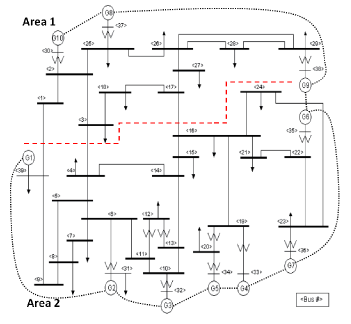
Figure 1: IEEE New England test power system.

In the simulations, the system is initially at a supply-demand balanced state with the nominal frequency. At time $t=0.5$ second, a step-wise increase of 33 MW of the loads at each of the buses 4, 12, and 20, amounting to a total power imbalance of 99 MW, causes the frequency to drop below the nominal frequency. The loads at other nodes do not change.

We conduct the simulations with the open source software PSAT and use the Euler-Forward method to discretize the ordinary differential equations and the Newton-Raphson method to solve the nonlinear system. We first evaluate the performance of PIAC on the network which is assumed as a single area. We compare the PIAC method with the GB, DAI and DecI control laws. For illustrations of the overshoot phenomena of other control laws, we refer to the simulation results of the literature published recently, e.g., [19, 35]. Then we implement the PIAC method in the network separated into two areas and show that the control actions of the areas are totally decoupled by PIAC as described in the subsection 4.2.

6.1 Numerical results of the Single-area implementation

Table 1. The control parameters
PIAC GB DAI DecI $k$ $k_{GB}$ $C_{i}$ $k_{i}$ $w_{ij}$ $k_{i}$ 5 60 $\frac{1}{39}$ 50 -20 50

In this subsection, the network is seen as a single area. The parameters for PIAC, GB, DAI and DecI are listed in Table 1. For the DAI method, the communication network is a weighted network as shown in Fig. 1 by the black dotted lines. The weight $w_{ij}$ for line $(i,j)$ is set as in Table 1 and $w_{ii}=-\sum_{(i,j)}w_{ij}$. The settings of these gain coefficients are chosen for a fair comparison in such a way that the slopes of the total control inputs, which reflect the required response time of the actuators, show close similarity (see Fig. 2d₁-2d₄).

Fig. 2 shows the comparison of the performances between the four control laws. Fig. 2a-2d show the responses of frequencies $\overline{\omega}_{i}=\omega_{i}+f^{*}$ for all $i\in\mathcal{V}_{M}$, virtual abstract frequency $\overline{\omega}_{s}=\omega_{s}+f^{*}$, relative frequency $\{\omega_{i}-\omega_{s},~{}i\in\mathcal{V}_{M}\}$ and control input $u_{s}$ respectively. The latter three illustrate the three-subprocesses decomposed from the dynamics of the system (1). Here, the responses of $\omega_{s}$ are obtained from (10) with $u_{s}$ as the total amount of control inputs of the PIAC and GB method respectively. It can be observed from Fig. 2a₁ and 2a₄ that all the control laws can restore the nominal frequency. However, the frequency deviation under the PIAC method is much smaller than under the other three control laws which introduce extra oscillations to the frequency. This is because the sum of control inputs of the GB, DAI, DecI method overshoot the desired value as Fig. 2d₂-2d₄ show, while the one of the PIAC method converges exponentially as Fig. 2$\text{d}_{1}$ shows. Because of the overshoot, the GB, DAI and DecI control laws require a maximum mechanical power input of about 140 MW from the 10 generators after the disturbance while the PIAC method only requires 99 MW in this simulation. This scenario is also well reflected in the response of the virtual frequency $\overline{\omega}_{s}$ as shown in Fig.2b₁-2b₄. Note that the convergences of the relative frequencies $\{\omega_{i}-\omega_{s},~{}i\in\mathcal{V}_{M}\}$ to zero as shown in Fig. 2c₁-2c₄ are the main concern of primary frequency control [12, 26]. Since the economic power dispatch is solved on-line, it can be observed in Fig. 2e₁-2e₂ that the marginal costs of all the controllers are the same during the transient phase under the control of PIAC and GB. In contrast with PIAC and GB, the marginal costs of DAI are not identical during the transient phase even though they achieve a consensus at the steady state. Because there are no control coordinations between the controllers in DecI, the marginal costs are not identical even at the steady state as shown in Fig. 2e₄. Since $u_{i}=\alpha_{i}\lambda$, the control inputs of the PIAC method and the GB method have similar dynamics as those of their marginal costs as shown in Fig. 2f₁-2f₂. Note that as shown in Fig. 2f₄, the control inputs of DecI are very close to each other because of the identical setting of $k_{i}$ and the small differences between the frequency deviations. As shown in Fig. 2f₁-Fig. 2f₃, the control inputs of some generators in the PIAC, GB and DAI control laws are small due to the high control prices.

We remark that the larger the gain coefficient $k_{GB}$ of the GB control law the larger are the oscillations of frequency deviations even though the frequencies converge to the nominal frequency faster. However, the control inputs of the PIAC method converge to the power imbalance faster under larger control gain $k$, which leads to smaller frequency deviations. As shown in Fig. 2a₁, the frequency drops about 0.4 Hz which can be even smaller when $k$ is larger. However, $k$ is related to the response time of the control devices and hence cannot be infinitely large. If the step-wise increase of the loads is too big and the gain coefficient $k$ is not large enough, i.e., the controllers cannot respond quickly enough, the frequency might become so low that they damage the synchronous machines.

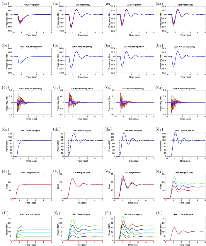
Figure 2: Comparison of the PIAC, GB, DAI, DecI control laws (single area implementation). In ($\text{d}_{1}$-$\text{d}_{4}$), the black dashed lines denote the power imbalance of the network. Only the marginal costs of the generators $\{2,3,4,5,7\}$ are shown in (e₃-e₄).

6.2 Numerical results of the Multi-area implementation

In this subsection, the network is separated into two areas by the red dashed line. All the parameters of the controllers are the same to the ones in the single-area implementation. There are 3 generators in area $A_{1}$ and 7 generators in the area $A_{2}$ i.e., $\mathcal{V}_{M_{1}}=\{30,37,38\},\mathcal{V}_{M_{2}}=\{31,32,33,34,35,36,39\}$. The boundary lines of area $A_{1}$ are in $\mathcal{E}_{A_{1}}=\{(1,39),(3,4),(17,16)\}$. As in subsection 6.1, the secondary frequency controllers are installed at the nodes of the generators. After the step-wise increase of the loads at buses 4, 12 and 20 with the total amount of 99 MW in the area $A_{2}$, the multi-area implementation of PIAC recovers the nominal frequency as shown in Fig. 3a and the power export deviation of area $A_{1}$ converges to zero as shown by the black dashed lines in Fig. 3b. Fig. 3b also shows that as the system converges to a new state, the power flows in the three line in $\mathcal{E}_{A_{1}}$ are different from the ones before the step-wise increase of the loads in area $A_{2}$. A characteristic of PIAC is that it decouples the control actions of the areas, which can be observed in Fig. 3c. Since the step-wise increase of the power loads at the buses 4, 12 and 20 happen in area $A_{2}$, the control inputs of area $A_{1}$ are zero and the power is balanced by the controllers in the area $A_{2}$. This shows that with the PIAC method, the power can be balanced locally in an area without influencing to its neighbors. This characteristic of PIAC is attractive for such a non-cooperative multi-area control of a power system that different areas might have different amount of renewable energy. It is fair for the area with a large amount of renewable energy to respond to the disturbance in its own area. As mentioned in subsection 4.2, this characteristic allows the controllers in different areas control the system in an asynchronous way at any time according to the power imbalance within the area.

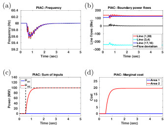
Figure 3: Multi-area implementation of PIAC.

7 Conclusion

In this paper, we proposed a secondary frequency control approach, called PIAC, to restore the nominal frequency of power systems with a minimized control cost. A main feature of PIAC is that the estimated power imbalance converges exponentially with a speed that only depends on a gain coefficient which can be tuned according to the sensitivity of the control devices. Hence PIAC eliminates the drawback of the traditional integral control based secondary frequency control approach, in which large control gain coefficients lead to an overshoot problem of the control inputs and small ones result in a large frequency deviation of the power systems. When implemented in a network with multiple areas, PIAC decouples the control actions of the areas such that the power supply and demand of an area can be balanced locally in the area without any influences to the neighbors. For the power systems with a large amount of integrated renewable energy, the large transient frequency deviation can be reduced by PIAC with advanced control devices and communication networks.

However, in practice, there is usually some noise from the measurement of frequency and time delays and even information losses in the communication. In addition, the resistance of the transmission lines cannot be neglected in some power networks, e.g., distribution grids of power systems or Micro-Grids. Hence, further investigation on the performance of PIAC on such a lossy power network with noisy measurements and time delays is needed. Further investigation is also required into the performance of PIAC in the power system with dynamic actuators.

Appendix A Preliminaries on DAE systems

Consider the following Differential Algebraic Equation (DAE) systems

$$\dot{x} =f(x,y),$$ (39a)

$$0 =g(x,y),$$ (39b)

where $x\in\mathbb{R}^{n}$ are state variables, $y\in\mathbb{R}^{m}$ are algebraic variables and $f:\mathbb{R}^{n}\times\mathbb{R}^{m}\rightarrow\mathbb{R}^{n}$ and $g:\mathbb{R}^{n}\times\mathbb{R}^{m}\rightarrow\mathbb{R}^{m}$ are twice continuously differentiable functions. (39a) and (39b) are differential and algebraic equations respectively. $(x(x_{0},y_{0},t),y(x_{0},y_{0},t))$ is the solution with the admissible initial conditions $(x_{0},y_{0})$ satisfying the algebraic constraints

$$0=g(x_{0},y_{0}).$$ (40)

and the maximal domain of a solution of (39) is denoted by $\mathcal{I}\subset\mathbb{R}_{\geq 0}$ where $\mathbb{R}_{\geq 0}=\{t\in\mathbb{R}|t\geq 0\}$.

Before presenting the Lyapunove/LaSalle stability criterion of the DAE system, we make the following two assumptions.

Assumption A.1: The DAE system possesses an equilibrium state $(x^{*},y^{*})$ such that $f(x^{*},y^{*})=0,~{}g(x^{*},y^{*})=0$.

Assumption A.2: Let $\Omega\subseteq\mathbb{R}^{n}\times\mathbb{R}^{m}$ be an open connected set containing $(x^{*},y^{*})$, assume (39b) is regular such that the Jacobian of $g$ with respect to $y$ is a full rank matrix for any $(x,y)\in\Omega$, i.e.,

$$\text{rank}(\nabla_{y}g(x,y))=m,~{}\forall(x,y)\in\Omega.$$

Assumption A.2 ensures the existence and uniqueness of the solutions of (39) in $\Omega$ over the interval $\mathcal{I}$ with the initial condition $(x_{0},y_{0})$ satisfying (40).

The following theorem provides a sufficient stability criterion of the equilibrium of DAE in (39).

Theorem A.1 (Lyapunov/LaSalle stability criterion [30, 15]): Consider the DAE system in (39) with assumptions A.1 and A.2, and an equilibrium $(x^{*},y^{*})\in\Omega_{H}\subset\Omega$. If there exists a continuously differentiable function $H:\Omega_{H}\rightarrow R$, such that $(x^{*},y^{*})$ is a strict minimum of $H$ i.e., $\nabla H|_{(x^{*},y^{*})}=0$ and $\nabla^{2}H|_{(x^{*},y^{*})}>0$, and $\dot{H}(x,y)\leq 0,~{}\forall(x,y)\in\Omega_{H}$, then the following statements hold:

(1). $(x^{*},y^{*})$ is a stable equilibrium with a local Lyapunov function $V(x,y)=H(x,y)-H(x^{*},y^{*})\geq 0$ for $(x,y)$ near $(x^{*},y^{*})$,

(2). Let $\Omega_{c}=\{(x,y)\in\Omega_{H}|H(x,y)\leq c\}$ be a compact sub-level set for some $c>H(x^{*},y^{*})$. If no solution can stay in $\{(x,y)\in\Omega_{c}|\dot{H}(x,y)=0\}$ other than $(x^{*},y^{*})$, then $(x^{*},y^{*})$ is asymptotically stable.

We refer to [30] and [15] for the proof of Theorem A.1.

References

- [1] M. Andreasson, D. V. Dimarogonas, H. Sandberg, and K. H. Johansson. Distributed control of networked dynamical systems: Static feedback, integral action and consensus. IEEE Transactions on Automatic Control, 59(7):1750–1764, 2014.
- [2] A. Araposthatis, S. Sastry, and P. Varaiya. Analysis of power-flow equation. International Journal of Electrical Power & Energy Systems, 3(3):115–126, 1981.
- [3] K. J. Aström and R. M. Murray. Feedback Systems: An introduction for scientists and Engineers. Princeton, NJ: Princeton UP, 2008.
- [4] T. Athay, R. Podmore, and S. Virmani. A practical method for the direct analysis of transient stability. IEEE Transactions on Power Apparatus and Systems, PAS-98(2):573–584, 1979.
- [5] A. W. Berger and F. C. Schweppe. Real time pricing to assist in load frequency control. IEEE Transactions on Power Systems, 4(3):920–926, Aug 1989.
- [6] Hassan Bevrani. Robust Power System Frequency Control. Springer, 2nd edition, 2014.
- [7] S. Boyd, N. Parikh, E. Chu, B. Peleato, and J. Eckstein. Distributed optimization and statistical learning via the alternating direction method of multipliers. Foundations and Trends in Machine Learning, 3(1):1–122, 2010.
- [8] R. A. Brualdi and H. J. Ryser. Combinatorial matrix theory, volume 39. Cambridge University Press, 1991.
- [9] L. Dong, Y. Zhang, and Z. Gao. A robust decentralized load frequency controller for interconnected power systems. ISA Transactions, 51(3):410–419, 2012.
- [10] F. Dörfler and F. Bullo. Synchronization and transient stability in power networks and nonuniform Kuramoto oscillators. SIAM Journal on Control and Optimization, 50(3):1616–1642, 2012.
- [11] F. Dörfler and S. Grammatico. Gather-and-broadcast frequency control in power systems. Automatica, 79:296 – 305, 2017.
- [12] F. Dörfler, J. W. Simpson-Porco, and F. Bullo. Breaking the hierarchy: distributed control and economic optimality in microgrids. IEEE Transactions on Control of Network Systems, 3(3):241–253, 2016.
- [13] O. I. Elgerd and C. E. Fosha. Optimum megawatt-frequency control of multiarea electric energy systems. IEEE Transactions on Power Apparatus and Systems, PAS-89(4):556–563, April 1970.
- [14] J. Han. From PID to active disturbance rejection control. IEEE Transactions on Industrial Electronics, 56(3):900–906, 2009.
- [15] D. J. Hill and I. M. Y. Mareels. Stability theory for differential algebraic systems with applications to power systems. IEEE Trans. Circuits and Systems, 37(11):1416–1423, 1990.
- [16] Ibraheem, P. Kumar, and D. P. Kothari. Recent philosophies of automatic generation control strategies in power systems. IEEE Transactions on Power Systems, 20(1):346–357, Feb 2005.
- [17] M.D. Ilić and J. Zaborszky. Dynamics and control of large electric power systems. John Wiley & Sons, 2000.
- [18] P. Kundur. Power system stability and control. McGraw-Hill, 1994.
- [19] N. Li, C. Zhao, and L. Chen. Connecting automatic generation control and economic dispatch from an optimization view. IEEE Transactions on Control of Networked Systems, 3(3):254–263, 2016.
- [20] F. Liu, Y. H. Song, J. Ma, S. Mei, and Q. Lu. Optimal load-frequency control in restructured power systems. IEE Proceedings - Generation, Transmission and Distribution, 150(1):87–95, 2003.
- [21] Y. Liu, Z. Qu, H. Xin, and D. Gan. Distributed real-time optimal power flow control in smart grid. IEEE Transactions on Power Systems, 32(5):3403–3414, 2017.
- [22] Jan Machowski, Janusz W. Bialek, and James R. Bumby. Power System Dynamics: Stability and Control. John Wiley & Sons. Ltd, 2nd edition, 2008.
- [23] Y. Mi, Y. Fu, C. Wang, and P. Wang. Decentralized sliding mode load frequency control for multi-area power systems. IEEE Transactions on Power Systems, 28(4):4301–4309, Nov 2013.
- [24] F. Milano. Power systems analysis toolbox. University of Castilla, Castilla-La Mancha, Spain, 2008.
- [25] D. K. Molzahn, F. D rfler, H. Sandberg, S. H. Low, S. Chakrabarti, R. Baldick, and J. Lavaei. A survey of distributed optimization and control algorithms for electric power systems. IEEE Transactions on Smart Grid, 8(6):2941–2962, Nov 2017.
- [26] A. E. Motter, S. A. Myers, M. Anghel, and T. Nishikawa. Spontaneous synchrony in power-grid networks. Nature Physics, 9(3):191–197, 2013.
- [27] C. De Persis and N. Monshizadeh. Bregman storage functions for microgrid control. IEEE Transactions on Automatic Control, 63(1):53–68, Jan 2018.
- [28] D. Rerkpreedapong, A. Hasanovic, and A. Feliachi. Robust load frequency control using genetic algorithms and linear matrix inequalities. IEEE Transactions on Power Systems, 18(2):855–861, May 2003.
- [29] P. Schavemaker and L. van der Sluis. Electrical power system essentials. John Wiley & Sons, 2008.
- [30] J. Schiffer and F. Dörfler. On stability of a distributed averaging PI frequency and active power controlled differential-algebraic power system model. In 2016 European Control Conference (ECC), pages 1487–1492, 2016.
- [31] J. Schiffer, T. Seel, J. Raisch, and T. Sezi. Voltage stability and reactive power sharing in inverter-based microgrids with consensus-based distributed voltage control. IEEE Transactions on Control Systems Technology, 24(1):96–109, 2016.
- [32] J. W. Simpson-Porco, F. Dörfler, and F. Bullo. Voltage collapse in complex power grids. Nature Communications, 7:10790, 2016.
- [33] J. W. Simpson-Porco, Q. Shafiee, F. Dörfler, J. C. Vasquez, J. M. Guerrero, and F. Bullo. Secondary frequency and voltage control of islanded microgrids via distributed averaging. IEEE Transactions on Industrial Electronics, 62(11):7025–7038, 2015.
- [34] S. J. Skar. Stability of multi-machine power systems with nontrivial transfer conductances. SIAM Journal on Applied Mathematics, 39(3):475–491, 1980.
- [35] S. Trip, M. Bürger, and C. De Persis. An internal model approach to (optimal) frequency regulation in power grids with time-varying voltages. Automatica, 64:240 – 253, 2016.
- [36] S. Trip and C. De Persis. Optimal frequency regulation in nonlinear structure preserving power networks including turbine dynamics: An incremental passivity approach. In 2016 American Control Conference (ACC), volume 2016-July, pages 4132–4137. IEEE, 2016.
- [37] D. Van Hertem. Usefulness of DC power flow for active power flow analysis with flow controlling devices. In 8th IEE International Conference on AC and DC Power Transmission (ACDC 2006), volume 2006, pages 58–62. IEE, 2006.
- [38] K. Vrdoljak, N. Perić, and I. Petrović. Sliding mode based load-frequency control in power systems. Electric Power Systems Research, 80(5):514 – 527, 2010.
- [39] Z. Wang, F. Liu, S. H. Low, C. Zhao, and S. Mei. Distributed frequency control with operational constraints, part ii: Network power balance. IEEE Transactions on Smart Grid, PP(99):1–1, 2017.
- [40] A. J. Wood and B. F. Wollenberg. Power generation, operation, and control. John Wiley & Sons, 2nd edition, 1996.
- [41] X. Wu, F. Dörfler, and M. R. Jovanovic. Input-Output analysis and decentralized optimal control of inter-area oscillations in power systems. IEEE Transactions on Power Systems, 31(3):2434–2444, 2016.
- [42] X. Wu and C. Shen. Distributed optimal control for stability enhancement of microgrids with multiple distributed generators. IEEE Transactions on Power Systems, 32(5):4045–4059, 2017.
- [43] X. Wu, C. Shen, and R. Iravani. A distributed, cooperative frequency and voltage control for microgrids. IEEE Transactions on Smart Grid, PP(99):1–1, 2017.
- [44] K. Xi, J. L. A. Dubbeldam, and H. X. Lin. Synchronization of cyclic power grids: equilibria and stability of the synchronous state. Chaos, 27(1):013109, 2017.
- [45] K. Xi, H. X. Lin, and J. H. van Schuppen. Power-imbalance allocation control of frequency control of power systems-a frequency bound for time-varying loads. In the 36th Chinese Control Conference, Dalian, China, pages 10528–10533, 2017.
- [46] Kaihua Xi, Johan L.A. Dubbeldam, Haixiang Lin, and Jan H. van Schuppen. Power-imbalance allocation control for secondary frequency control of power systems. IFAC-PapersOnLine, 50(1):4382 – 4387, 2017. 20th IFAC World Congress.
- [47] C. Zhao, E. Mallada, and F. Dörfler. Distributed frequency control for stability and economic dispatch in power networks. In 2015 American Control Conference (ACC), pages 2359–2364, 2015.
- [48] C. Zhao, E. Mallada, S. Low, and J. Bialek. A unified framework for frequency control and congestion management. In 2016 Power Systems Computation Conference (PSCC), pages 1–7, 2016.
- [49] C. Zhao, U. Topcu, N. Li, and S. Low. Design and stability of load-side primary frequency control in power systems. IEEE Transactions on Automatic Control, 59(5):1177–1189, 2014.