New approximation for GARCH parameters estimate Yakoub BOULAROUK¹ , Nasr-eddine HAMRI^{1 1} Institute of Science and Technology, Melilab laboratory, University Center of Mila, Algeria

Abstract: This paper presents a new approach for the optimization of GARCH parameters estimation. Firstly, we propose a method for the localization of the maximum. Thereafter, using the methods of least squares, we make a local approximation for the projection of the likelihood function curve on two dimensional planes by a polynomial of order two which will be used to calculate an estimation of the maximum.

Keyword GARCH Process, Likelihood function, Least squares.

1 Introduction

The modeling of time series is applied today in fields as diverse (econometrics, medicine or demographics….). As it is a crucial step in the study of time series, it has undergone a great evolution during the last fifty years and several models of representation have been proposed.
In 1982, Engle [4] proposed the conditionally heteroskedastic autoregressive (ARCH) model, which allowed the conditional variance to change as a function of past errors over time, while leaving the variance unconditional constant. This model has already proved useful in the modeling of several phenomenas. In Engle [4, 5] and Engle and Kraft [6], models for the inflation rate are constructed recognizing that the uncertainty of inflation tends to change over time. In 1984, Weiss [14] considered the ARMA models with ARCH errors. He used these models for the modeling of sixteen US microeconomic time series.
In 1986, Bollerslev [1] proposed a generalization of these ARCH models to the Generalized AutoRegressive Conditional Heteroskedasticity (GARCH) models, whose the variance in the present depends on its past and the process past. As it studied the conditions of stationarity and the structure of the autocorrelations for this class of models.
The GARCH family contains a number of parameters which must be estimated on actual data for empirical applications. The estimation of the parameters returns to calculate the maximum of the log-likelihood function which is non-linear, this leads to the use of non-linear optimization methods. Several optimization methods are used, including The Nelder-Mead method, BGFS method and others :

• Nelder and Mead [11] introduced their method using only

  the likelihood function values. Altough their method is relatively slow, it’s robust and leads to results for the non differentiable functions. In their turn Fletcher and Reeves [9] have introduced the method of the conjugate gradient which does not store matrix.

• In 1970 Broyden [3], Fletcher [8], Goldfarb [10] and Shanno [12] have published simultaneously the method entitled quasi-Newton (noted BFGS), which uses the values and the gradients of function to construct an image of the surface to optimize.

• In 1990 David M. Gay [7] have published a technical report in which he proposed a method intitiled optimization using PORT routines (noted OPR).

It is common knowledge among practitioners that the GARCH parameters are numerically difficult to estimate in empirical applications. The existant numerical algorithm can easily fail, or converge to erratic solutions. Therefore, the resulting fitted parameters must be examined with a healthy dose of scepticism. In this work, we propose a new algorithm in which we exploit the asymptotic convexity of the likelihood function. We will develop a method to locate the maximum value instead of using the confidence intervals resulting from asymptotic normality of the estimated parameters thereafter and as in [2], we approach the likelihood function by a quadratic form that we use to calculate an approximation of the maximum.

2 The GARCH model and its likelihood function

The GARCH$(p,q)$ process was introduced by Bollerslev [1] as solution for the system of equations:

$$\left\{\begin{array}[]{ll}&X_{t}=\sigma_{t}\cdot\varepsilon_{t},\\ &\sigma_{t}^{2}=\omega+\Sigma_{i=1}^{p}\alpha_{i}X_{t-i}^{2}+\Sigma_{j=1}^{q}\beta_{j}\sigma_{t-j}^{2}.\\ \end{array}\right.$$ (2.1)

Let’s note $\theta=(\omega,\alpha_{1},...,\alpha_{p},\beta_{1},...,\beta_{q})\in\mathbb{R}^{p+q+1}$ the vector of unknown parameters, with $\omega>0$, $\alpha_{i}\geq 0$ for $i=1,p-1$, $\beta_{j}\geq 0$ for $j=1,q-1$, $\alpha_{p},\beta_{q}$ strictly positive. The $(\varepsilon_{t})_{t\geq 0}$ is a sequence of normal random independent and identically distributed satisfying the standard assumptions $\mathrm{E}(\varepsilon_{t})=0$ and $\mbox{Var}(\varepsilon_{t})=1$. The ARCH$(q)$ is an GARCH$(0,q)$
The conditional likelihood of $X$ expresses as, up to an additional constant,

$$L_{n}(\theta) = -\frac{1}{2}\sum^{n}_{t=1}q_{t}(\theta).$$

with $$q_{t}(\theta)=log(\sigma_{t}^{2})+\sigma_{t}^{-2}X_{t}^{2}$$

The quasi-likelihood $\widehat{L}_{n}$ is obtained by plugging in $L_{n}$ the approximations $\widehat{\sigma}_{t}^{2}=\sigma_{t}^{2}(X_{t},...,X_{1},u_{n})$, where $u=(u_{n})_{n\in\mathbb{N}}$ is different of zero only for finitely many $n\in\mathbb{N}$,

$$\widehat{L}_{n}(\theta) = -\frac{1}{2}\sum^{n}_{t=1}\widehat{q}_{t}(\theta).$$

with $$\widehat{q}_{t}(\theta)=log(\widehat{\sigma}_{t}^{2})+\widehat{\sigma}_{t}^{-2}X_{t}^{2}$$

Remark that unobserved values $(X_{t},t\leq 0)$ have to be fixed a priori equal to $(u_{n})_{n\in N}$ in the quasi-likelihood $\widehat{L}_{n}$. In the next proposition, we give a necessary and sufficient condition for the process stationarity.

Proposition 2.1.

The GARCH( $p,q$) process as defined in (2.1) is wide-sense stationary with $E(\varepsilon_{t})=0$, $\mbox{Var}(\varepsilon_{t})=\alpha_{0}(\Sigma_{i=1}^{p}\alpha_{i}+\Sigma_{i=1}^{q}\beta_{i})^{-1}$ and $\mbox{Cov}(\varepsilon_{t},\varepsilon_{s})=0$ for $t\neq s$ if and only if

$$\Sigma_{i=1}^{p}\alpha_{i}+\Sigma_{i=1}^{q}\beta_{i}<1$$ (2.2)

Proof 1.

This result is proved by Bollerslev in [1].

The condition (2.2) implies that $0\leq\alpha_{i}<1,\forall i=1,p$ and $0\leq\beta_{j}<1,\forall j=1,q$. Else, we define the stationarity set

$$\Theta_{0}=\{\theta\in\mathbb{R}^{p+q+1},\theta_{i}\geq 0,\Sigma_{i=1}^{p}\alpha_{i}+\Sigma_{i=1}^{q}\beta_{i}<1\}$$ (2.3)

3 Necessary tools

3.1 Convexity

W.C. Ip and al. [13] have proved the convexity of the negative likelihood function in the asymptotic sense for GARCH models. This property allows us the local approximation of this function in the Neighborhood of its minimum by a polynomial of degree two.

Proposition 3.1.

Suppose $\Theta_{1}$ is an arbitrary compact, convex subset of $\Theta_{0}$ and $f^{{}^{\prime}}_{n}(\theta,\varpi)$ the second derivative of $L_{n}(\theta)$. Then there exist a constant $C>0$ and a set $\Omega$ with $P(\Omega)=1$ satisfying that for each $\varpi\in\Omega$ and $\theta\in\Theta_{1}$, there is a positive integer $N(\varpi,\theta)$ such that

$$\upsilon^{T}f^{{}^{\prime}}_{n}(\theta,\varpi)\upsilon\geq C\upsilon^{T}\upsilon,\forall n\geq N(\varpi,\theta),\upsilon\in R^{p+q+1}.$$ (3.1)

3.2 Localisation method

In this part, we propose a method to search for a block of the form $\Pi_{i=1}^{p+q+1}]\underline{\theta_{i}},\overline{\theta_{i}}[$ containing the maximum sought-after. The method is based on the principle of dichotomy applied for projections of the likelihood function on a plane with dimension two, we follow the steps

1. We search a point $\overline{\omega}$ that verifie $\widehat{L_{1,n}}^{{}^{\prime}}(\omega,0.5,...,0.5)>0$, where $\widehat{L_{i,n}}^{{}^{\prime}}$ is the $i$ order derivative of the likelihood function with respect to $\omega$.

2. We put $\underline{\theta_{i}}=0.0001,\forall{i=1,p+q+1}$ and $\overline{\theta_{1}}=\overline{\omega},\overline{\theta_{i}}=0.9999,\forall{i=2,p+q+1}$

3. $\forall{i=1,p+q+1}$
   

   • if $\widehat{L^{{}^{\prime}}_{i,n}}\big{(}\underline{\theta_{1}},...,\underline{\theta_{i}},....,\underline{\theta}_{p+q+1}\big{)}\widehat{L_{i,n}}^{{}^{\prime}}\big{(}\underline{\theta_{1}},....,(\underline{\theta}_{i}+\overline{\theta}_{i})/2,....,\underline{\theta}_{p+q+1}\big{)}<0$ then we replace $\overline{\theta_{i}}$ by $(\underline{\theta}_{i}+\overline{\theta}_{i})/2$

   • else if $\widehat{L^{{}^{\prime}}_{i,n}}\big{(}\underline{\theta_{1}},...,\underline{\theta_{i}},....,\underline{\theta_{p+q+1}}\big{)}\widehat{L_{i,n}}^{{}^{\prime}}\big{(}\underline{\theta_{1}},....,(\underline{\theta}_{i}+\overline{\theta}_{i})/2,....,\underline{\theta}_{p+q+1}\big{)}>0$ we replace $\underline{\theta}_{i}$ by $(\underline{\theta}_{i}+\overline{\theta}_{i})/2$

We repeat the step $3$ until $\overline{\theta}_{i}-\underline{\theta}_{i}\leq 0.05,\forall{i=1,p+q+1}$.

4 Calculation procedure

To calculate the maximum likelihood, one passes by the following steps

1. Calculate confidence intervals for the unknown parameters using the localisation method.

2. Make a subdivision of $m$ elements $(\theta_{ij})_{j=1,m}$ for all the confidence intervals $(I_{i})_{i=1,p+q+1}$.

3. Calculate the function values $\big{[}l_{n}(\theta_{j})\big{]}_{j=1,m}$ where $\theta_{j}=(\theta_{ij})_{i=1,p+q+1}=(\omega_{j},\alpha_{1j},...,\alpha_{pj},\beta_{1j},...,\beta_{qj})$, Which is a cut for the curve of the likelihood function on the diagonal plane of the confidence region.

4. Numerical approximation for the orthogonal projection of the log likelihood function cut by polynomials of order two taking the form $a_{0}+a_{1}\theta_{i}+a_{2}\theta_{i}^{2}$: we use the least squares method.

5. Calculate these maximum.

5 Example of application ARCH(1)

The $ARCH(1)$ process is presented as solution of the system

$$\left\{\begin{array}[]{ll}&X_{t}=\sigma_{t}\cdot\varepsilon_{t},\\ &\sigma_{t}^{2}=\omega+\alpha_{1}X_{t-i}^{2}.\\ \end{array}\right.$$ (5.1)

where $\omega>0$ and $0<\alpha_{1}<1$.
Let be $(x_{t})_{t=1,100}$ the simulated first order conditionally heteroskedastic autoregressive time series $ARCH(1)$ with ($\omega=0.8$ and $\alpha_{1}=0.3$) presented by the table 3.

Time $t$	1	2	3	4	5	6	7	8	9	10
$x_{t}$	-1.348	-0.05	-0.063	2.055	0.815	1.893	-2.277	-1	0.782	0.351
Time $t$	11	12	13	14	15	16	17	18	19	20
$x_{t}$	-0.791	-2.24	1.723	0.667	-0.015	0.464	0.22	-0.737	0.434	0.643
Time $t$	21	22	23	24	25	26	27	28	29	30
$x_{t}$	-0.259	-0.313	0.907	1.268	-0.888	-1.376	-1.367	-0.805	0.528	-0.813
Time $t$	31	32	33	34	35	36	37	38	39	40
$x_{t}$	-1.89	-2.051	1.94	1.643	-1.071	-0.336	1.085	-0.766	1.59	0.993
Time $t$	41	42	43	44	45	46	47	48	49	50
$x_{t}$	-1.162	2.985	-0.1	-0.732	0.391	0.132	-2.224	-0.271	-0.336	-1.606
Time $t$	51	52	53	54	55	56	57	58	59	60
$x_{t}$	0.509	-0.026	0.468	-1.626	1.219	0.315	-0.416	0.636	0.848	-1.011
Time $t$	61	62	63	64	65	66	67	68	69	70
$x_{t}$	1.152	0.085	-0.114	-0.744	1.456	-0.243	-0.332	-0.078	0.678	1.668
Time $t$	71	72	73	74	75	76	77	78	79	80
$x_{t}$	-1.499	-1.347	-0.886	-0.578	-1.94	0.156	-0.082	-0.173	-0.63	-0.677
Time $t$	81	82	83	84	85	86	87	88	89	90
$x_{t}$	-0.397	1.283	0.479	-1.035	-0.917	1.054	-0.605	0.412	-1.055	0.994
Time $t$	91	92	93	94	95	96	97	98	99	100
$x_{t}$	-0.259	-0.313	0.907	1.268	-0.888	-1.376	-1.367	-0.805	0.528	-0.813

Table 1: Table of the time serie $x_{t}$.

We plot this time series as function of time

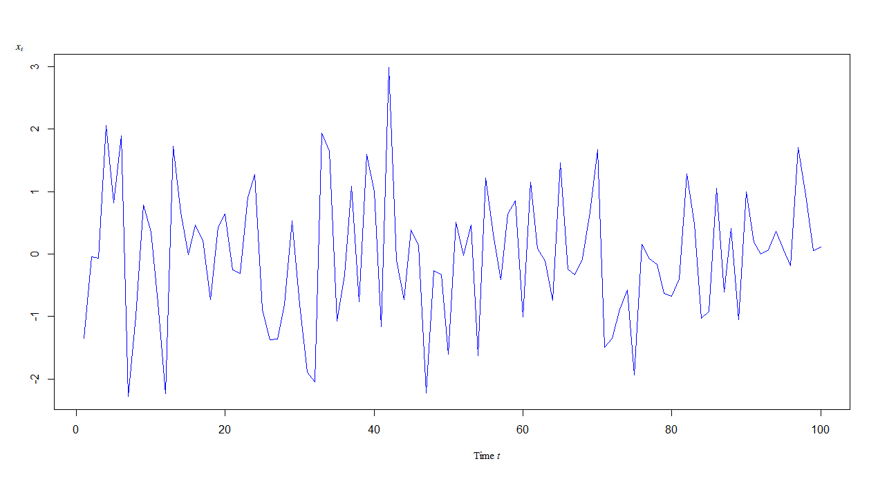
Figure 1: The time serie $x_{t}$.

The log likelihood of an $ARCH(1)$ process is given by

$$L_{n}(\theta) = -\frac{1}{2}\sum^{n}_{t=1}\Big{[}log\big{(}\omega+\alpha_{1}X_{t-1}^{2}\big{)}^{2}+\big{(}\omega+\alpha_{1}X_{t-1}^{2}\big{)}^{-2}X_{t}^{2}\Big{]}.$$

to obtain $\widehat{L}_{n}$ we replace $(X_{-i}),i\geq 0$ by zero.
Now, we proceed to the calculation of the maximum likelihood using our method

1. We remark that $\widehat{L_{n,1}^{{}^{\prime}}}(0.8001,0.5)>0$, therefore $\omega\in]0.0001,0.8001[$.

   $w$	0.0001	0.2001	0.4001	0.6001	0.8001
   $\widehat{L_{n,1}^{{}^{\prime}}}(w,0.5)$	-7613853	-455.4789	-93.72643	-19.2947	5.967303

   Table 2: Table of the derivative values.

2. Using the localisation procedure, we find that the region $]0.7751000,0.8501000[\times]0.2813219,0.3625687[$ contains the maximum.

3. We calculate the function values on the diagonal plane of the confidence region, which give the table 3.

   $\omega$	0.7751	0.7759	0.7766	0.7774	0.7781	0.7789	0.7796	0.7804	0.7812	0.7819
   $\alpha_{1}$	0.2813	0.2821	0.283	0.2838	0.2846	0.2854	0.2862	0.2871	0.2879	0.2887
   $\widehat{L}_{n}(\omega,\alpha_{1})$	109.257	109.251	109.245	109.239	109.233	109.227	109.222	109.217	109.212	109.207
   $\omega$	0.7827	0.7834	0.7842	0.7849	0.7857	0.7865	0.7872	0.788	0.7887	0.7895
   $\alpha_{1}$	0.2895	0.2903	0.2912	0.292	0.2928	0.2936	0.2945	0.2953	0.2961	0.2969
   $\widehat{L}_{n}(\omega,\alpha_{1})$	109.202	109.198	109.194	109.19	109.186	109.182	109.179	109.176	109.173	109.17
   $\omega$	0.7903	0.791	0.7918	0.7925	0.7933	0.794	0.7948	0.7956	0.7963	0.7971
   $\alpha_{1}$	0.2977	0.2986	0.2994	0.3002	0.301	0.3018	0.3027	0.3035	0.3043	0.3051
   $\widehat{L}_{n}(\omega,\alpha_{1})$	109.168	109.165	109.163	109.161	109.159	109.158	109.156	109.155	109.154	109.153
   $\omega$	0.7978	0.7986	0.7993	0.8001	0.8009	0.8016	0.8024	0.8031	0.8039	0.8046
   $\alpha_{1}$	0.3059	0.3068	0.3076	0.3084	0.3092	0.3100	0.3109	0.3117	0.3125	0.3133
   $\widehat{L}_{n}(\omega,\alpha_{1})$	109.153	109.152	109.152	109.152	109.152	109.152	109.153	109.153	109.154	109.155
   $\omega$	0.8054	0.8062	0.8069	0.8077	0.8084	0.8092	0.8099	0.8107	0.8115	0.8122
   $\alpha_{1}$	0.3141	0.315	0.3158	0.3166	0.3174	0.3183	0.3191	0.3199	0.3207	0.3215
   $\widehat{L}_{n}(\omega,\alpha_{1})$	109.156	109.157	109.159	109.161	109.162	109.164	109.167	109.169	109.171	109.174
   $\omega$	0.813	0.8137	0.8145	0.8153	0.816	0.8168	0.8175	0.8183	0.819	0.8198
   $\alpha_{1}$	0.3224	0.3232	0.324	0.3248	0.3256	0.3265	0.3273	0.3281	0.3289	0.3297
   $\widehat{L}_{n}(\omega,\alpha_{1})$	109.177	109.18	109.183	109.186	109.19	109.193	109.197	109.201	109.205	109.21
   $\omega$	0.8206	0.8213	0.8221	0.8228	0.8236	0.8243	0.8251	0.8259	0.8266	0.8274
   $\alpha_{1}$	0.3306	0.3314	0.3322	0.333	0.3338	0.3347	0.3355	0.3363	0.3371	0.3379
   $\widehat{L}_{n}(\omega,\alpha_{1})$	109.214	109.218	109.223	109.228	109.233	109.238	109.244	109.249	109.255	109.26
   $\omega$	0.8281	0.8289	0.8296	0.8304	0.8312	0.8319	0.8327	0.8334	0.8342	0.8349
   $\alpha_{1}$	0.3388	0.3396	0.3404	0.3412	0.3421	0.3429	0.3437	0.3445	0.3453	0.3462
   $\widehat{L}_{n}(\omega,\alpha_{1})$	109.266	109.272	109.279	109.285	109.291	109.298	109.305	109.312	109.319	109.326
   $\omega$	0.8357	0.8365	0.8372	0.838	0.8387	0.8395	0.8403	0.841	0.8418	0.8425
   $\alpha_{1}$	0.347	0.3478	0.3486	0.3494	0.3503	0.3511	0.3519	0.3527	0.3535	0.3544
   $\widehat{L}_{n}(\omega,\alpha_{1})$	109.333	109.341	109.349	109.356	109.364	109.372	109.38	109.389	109.397	109.406
   $\omega$	0.8433	0.844	0.8448	0.8456	0.8463	0.8471	0.8478	0.8486	0.8493	0.8501
   $\alpha_{1}$	0.3552	0.356	0.3568	0.3576	0.3585	0.3593	0.3601	0.3609	0.3617	0.3626
   $\widehat{L}_{n}(\omega,\alpha_{1})$	109.414	109.423	109.432	109.441	109.45	109.46	109.469	109.479	109.488	109.498

   Table 3: Table of $(\omega,\alpha_{1}),\widehat{L}_{n}(\omega,\alpha_{1})$.

4. Using the least squares method, we calculate approximations of $\big{(}\omega_{i},\widehat{L}_{n}(\omega_{i},\alpha_{1i})\big{)}_{i=1,100}$ and $\big{(}\alpha_{1i},\widehat{L}_{n}(\omega_{i},\alpha_{1i})\big{)}_{i=1,100}$ the orthogonal projections of the likelihood function curve cut $\big{(}\omega_{i},\alpha_{1i},\widehat{L}_{n}(\omega_{i},\alpha_{1i})\big{)}_{i=1,100}$ on the planes $(o,\omega,ln(\omega,\alpha_{1}))$, $(o,\alpha_{1},ln(\omega,\alpha_{1}))$ respectively.
   

   • The approximation function for the likelihood function Curve cut projection on the plane $(o,\omega,ln(\omega,\alpha_{1}))$ is

     $f(\theta)=143.7092\omega^{2}-230.1460\omega+143.7092$;

     the maximum of this function is $230.1460/(2*143.7092)=0.8007353$.
     In the Figure 2, we represent the projection of the cut of the likelihood function on the plane $(o,\omega,ln(\omega,\alpha_{1}))$ and its approximation

     

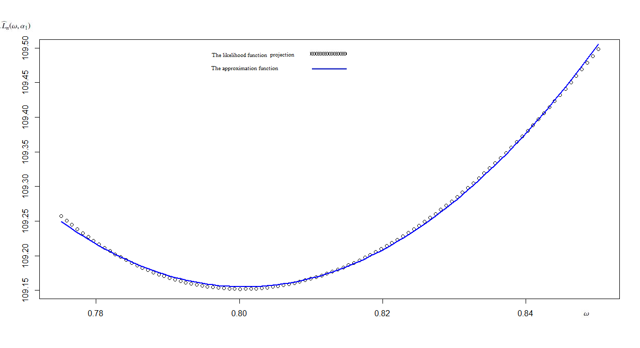
     Figure 2: The projection of the cut of the likelihood function on the plane $(o,\omega,ln(\omega,\alpha_{1}))$ and its approximation

   • The approximation function for the likelihood function curve cut projection on the plane $(o,\alpha,ln(\omega,\alpha_{1}))$ is

     $f(\theta)=120.8546\alpha_{1}^{2}-75.7028\alpha_{1}+122.4599$;

     the maximum value of this function is $75.7028/(2*120.8546)=0.3090923$.
     

     The Figure 3 illustrates the projection of the cut of the likelihood function on the plane $(o,\omega,ln(\omega,\alpha_{1}))$ and its approximation

     

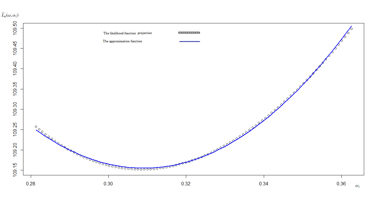
     Figure 3: The projection of the cut of the likelihood function on the plane $(o,\alpha_{1},ln(\omega,\alpha_{1}))$ and its approximation

6 Numerical comparaison study

To illustrate the performance of the proposed method, we compare it with some popular methods (BGFS, Simplex and OPR) usually used in the Time series parameters calculation. We applied these methods to $1000$ independent replications of two ARCH$(1)$ process (one with $\omega=1.2$, $\alpha=0.6$ end the other with $\omega=0.7$, $\alpha=0.4$ for different sample size $n=100$, $n=200$ and $n=300$, thereafter we compute the root-mean-square error (RMSE) $RMSE(\omega)+RMSE(\alpha_{1})$ of the resulting estimation, the results are presented in Table 4.

		$\omega=1.2,\alpha_{1}=0.6$				$\omega=0.7,\alpha_{1}=0.4$
	Sample size	Our Method	BGFS	Simplex	OPR	Our Method	BGFS	Simplex	OPR
	100	0.485	0.607	0.609	0.609	0.798	0.804	0.807	0.807
	200	0.345	0.368	0.368	0.368	0.747	0.752	0.752	0.752
	300	0.292	0.300	0.300	0.300	0.742	0.743	0.743	0.743

Table 4: Root Mean Square Error of our method, BGFS, Simplex and OPR for an ARCH$(1)$ processes.

Conclusion of the numerical comparaison results: On the one hand, it is clear that the RMSE decreases as the sample size increases, which validates the theoretical results (consistency of the estimators). On the other hand, Table 4 show that our method provides more accurate estimation than the BGFS, Simplex and OPR methods.

References

- [1] Bollerslev, T. (1986), Generalised autoregressive conditional heteroscedasticity, Journal of Econometrics, 31, 307-327.
- [2] Y. Boularouk and K. Djeddour (2015), New approximation for ARMA parameters estimate, Mathematics and Computers in Simulation, 118,116-122.
- [3] Broyden, C. G. (1970), The convergence of a class of double-rank minimization algorithms, Journal of the Institute of Mathematics and Its Applications, 6, 76-90.
- [4] Engle, R.F. (1982), Autoregressive conditional heteroskedasticity with estimates of the variance of U.K. inflation, Econometrica 50, 987-1008.
- [5] Engle, R.F. (1983), Estimates of the variance of U.S. inflation based on the ARCH model, Journal of Money Credit and Banking 15, 286-301.
- [6] Engle, R.F. and D. Kraft (1983), Multiperiod forecast error variances of inflation estimated from ARCH models, in: A. ZeUner, ed., Applied time series analysis of economic data (Bureau of the Census, Washington, DC) 293-302.
- [7] David M. Gay (1990), Usage summary for selected optimization routines. Computing Science Technical Report 153, AT and T Bell Laboratories, Murray Hill.
- [8] Fletcher, R. (1970), A New Approach to Variable Metric Algorithms, Computer Journal, 13, 3, 317-322
- [9] Fletcher, R. Reeves, C. M. (1964), Function minimization by conjugate gradients, The Computer Journal, Vol. 7, 2, 149-154.
- [10] Goldfarb, D. (1970),A Family of Variable Metric Methods Derived by Variational Means Maths. Comput., 24, 23-26.
- [11] Nelder, J. A. Mead, R. (1965), A Simplex Method for Function Minimization. Comput. J. 7, 308-313.
- [12] Shanno, David, F. Kettler, Paul C. (1970), Optimal conditioning of quasi-Newton methods, Math. Comput. 24, 111, 657-664.
- [13] W.C. Ipa, Heung Wonga, J.Z. Panb, , , D.F. Lic (2006), The asymptotic convexity of the negative likelihood function of GARCH models. Computational Statistics and Data Analysis, Volume 50, Issue 2, 30 January 2006, 311-331.
- [14] Weiss, A.A. (1984), ARMA models with ARCH errors. J. Time Ser. Anal., 5, 2, 129-143.