Degree-optimal Moving Frames for Rational Curves

Abstract

A moving frame at a rational curve is a basis of vectors moving along the curve. When the rational curve is given parametrically by a row vector $\mathbf{a}$ of univariate polynomials, a moving frame with important algebraic properties can be defined by the columns of an invertible polynomial matrix $P$, such that $\mathbf{a}P=[\gcd(\mathbf{a}),0\ldots,0]$. A degree-optimal moving frame has column-wise minimal degree, where the degree of a column is defined to be the maximum of the degrees of its components. Algebraic moving frames are closely related to the univariate versions of the celebrated Quillen-Suslin problem, effective Nullstellensatz problem, and syzygy module problem. However, this paper appears to be the first devoted to finding an efficient algorithm for constructing a degree-optimal moving frame, a property desirable in various applications. We compare our algorithm with other possible approaches, based on already available algorithms, and show that it is more efficient. We also establish several new theoretical results concerning the degrees of an optimal moving frame and its components. In addition, we show that any deterministic algorithm for computing a degree-optimal algebraic moving frame can be augmented so that it assigns a degree-optimal moving frame in a $GL_{n}(\mathbb{K})$-equivariant manner. This crucial property of classical geometric moving frames, in combination with the algebraic properties, can be exploited in various problems.

Keywords: rational curves, moving frames, Quillen-Suslin theorem, effective univariate Nullstellensatz, Bézout identity and Bézout vectors, syzygies, $\mu$-bases.

MSC 2010: 12Y05, 13P10, 14Q05, 68W30.

1 Introduction

Let $\mathbb{K}[s]$ denote a ring of univariate polynomials over a field $\mathbb{K}$ and let $\mathbb{K}[s]^{n}$ denote the set of row vectors of length $n$ over $\mathbb{K}$. Let $GL_{n}(\mathbb{K}[s])$ denote the set of invertible $n\times n$ matrices over $\mathbb{K}[s]$, or equivalently, the set of matrices whose columns are point-wise linearly independent over the algebraic closure $\overline{\mathbb{K}}$.

A nonzero row vector $\mathbf{a}\in\mathbb{K}[s]^{n}$ defines a parametric curve in $\mathbb{K}^{n}$. The columns of a matrix $P\in GL_{n}(\mathbb{K}[s])$ assign a basis of vectors in $\mathbb{K}^{n}$ at each point of the curve. In other words, the columns of the matrix can be viewed as a coordinate system, or a frame, that moves along the curve. To be of interest, however, such assignment should not be arbitrary, but instead be related to the curve in a meaningful way. In this paper, we require that $\mathbf{a}\,P=[\gcd(\mathbf{a}),0,\dots,0]$, where $\gcd(\mathbf{a})$ is the monic greatest common divisor of the components of $\mathbf{a}$. We will call a matrix $P$ with the above property an algebraic moving frame at $\mathbf{a}$. We observe that for any nonzero monic polynomial $\lambda(s)$, a moving frame at $\mathbf{a}$ is also a moving frame at $\lambda\mathbf{a}$. Therefore, we can obtain an equivalent construction in the projective space $\mathbb{PK}^{n-1}$ by considering only polynomial vectors $\mathbf{a}$ such that $\gcd(\mathbf{a})=1$. Then $P$ can be thought of as an element of $PGL_{n}(\mathbb{K}[s])=GL_{n}(\mathbb{K}[s])/{cI}$, where $c\neq 0\in\mathbb{K}$ and $I$ is an identity matrix. A canonical map of $\mathbf{a}$ to any of the affine subsets $\mathbb{K}^{n-1}\subset\mathbb{PK}^{n-1}$ produces a rational curve in $\mathbb{K}^{n}$, and $P$ assigns a projective moving frame at $\mathbf{a}$. This paper is devoted to degree-optimal algebraic moving frames – frames that column-wise have minimal degrees, where the degree of a column is defined to be the maximum of the degrees of its components (see Definitions 1 and 4).

Algebraic moving frames appeared in a number of important proofs and constructions under a variety of names. For example, in the constructive proofs of the celebrated Quillen-Suslin theorem [21], [31], [7], [35], [32], [17], given a polynomial unimodular $m\times n$ matrix ${\bf A}$, one constructs a unimodular matrix $P$ such that ${\bf A}P=[I_{m},\bf{0}]$, where $I_{m}$ is an $m\times m$ identity matrix. In the univariate case with $m=1$, the matrix $P$ is an algebraic moving frame. However, the above works were not concerned with the problem of finding $P$ of optimal degree for every input ${\bf A}$. Under the same assumptions on ${\bf A}$, a minimal multiplier, defined in Section 3 of [5], is a degree-optimal algebraic moving frame. However, the paper [5] was not concerned with constructing minimal multipliers, and a direct algorithm for computing them was not introduced. In Section 6, we discuss a two-step approach, consisting of constructing a non-optimal moving frame and then performing a degree-reduction procedure. We show that it is less efficient than the direct approach developed in the current paper. An alternative direct approach for computing degree-optimal moving frames is in the dissertation of the second author ([27], Sections 5.9 and 5.10) This approach is based on computing the term-over-position (TOP) Gröbner basis of a certain module over $\mathbb{K}[s]$, and when standard TOP Gröbner basis algorithms for modules are employed, it is less efficient than the algorithm in the current paper. Optimizations, based on the structure of the particular problem, are possible and are the subject of a forthcoming publication.

A very important area of applications where, according to our preliminary studies, utilization of degree-optimal moving frames is beneficial, is the control theory. In particular, the use of degree-optimal frames can lower differential degrees of “flat outputs” (see, for instance, Polderman and Willems [36], Martin, Murray and Rouchon [33], Fabiańska and Quadrat [17], Antritter and Levine [2], Imae, Akasawa, and Kobayashi [28]). Another interesting application of algebraic frames can be found in the paper [16] by Elkadi, Galligo and Ba, devoted to the following problem: given a vector of polynomials with gcd 1, find small degree perturbations so that the perturbed polynomials have a large-degree gcd. As discussed in Example 3 of [16], the perturbations produced by the algorithm presented in this paper do not always have minimal degrees. It would be worthwhile to study if the usage of degree-optimal moving frames can decrease the degrees of the perturbations.

Obviously, the first column of an algebraic moving frame $P$ at $\mathbf{a}$ is a Bézout vector of $\mathbf{a}$; that is, a vector comprised of the coefficients appearing in the output of the extended Euclidean algorithm. In Proposition 9, we prove that the last $n-1$ columns of $P$ comprise a point-wise linearly independent basis of the syzygy module of $\mathbf{a}$. In Theorem 1, we show that a matrix $P$ is a degree-optimal moving frame at $\mathbf{a}$ if and only if the first column of $P$ is a Bézout vector of $\mathbf{a}$ of minimal degree, and the last $n-1$ columns form a basis of the syzygy module of $\mathbf{a}$ of optimal degree, called a $\mu$-basis [13]. The concept of $\mu$-bases, along with several related concepts such as moving lines and moving curves, have a long history of applications in geometric modeling, originating with works by Sederberg and Chen [37], Cox, Sederberg and Chen [13]. Further development of this topic appeared in [8, 38, 30, 39].

One may attempt to construct an optimal moving frame by putting together a minimal-degree Bézout vector and a $\mu$-basis. Indeed, algorithms for computing $\mu$-bases are well-developed. The most straightforward (and computationally inefficient) approach consists of computing the reduced Gröbner basis of the syzygy module with respect to a term-over-position monomial ordering. More efficient algorithms have been developed by Cox, Sederberg, and Chen[13], Zheng and Sederberg [43], Chen and Wang [9] for the $n=3$ case, and by Song and Goldman [38] and Hong, Hough and Kogan [26] for arbitrary $n$. The problem of computing a $\mu$-basis also can be viewed as a particular case of the problem of computing optimal-degree kernels of $m\times n$ polynomial matrices of rank $m$ (see for instance Beelen [6], Antoniou, Vardulakis, and Vologiannidis [1], Zhou, Labahn, and Storjohann [45] and references therein). On the contrary, our literature search did not yield any articles devoted to the problem of finding an efficient algorithm for computing a minimal-degree Bézout vector. Of course, one can compute such a vector by a brute-force method, namely by searching for a Bézout vector of a fixed degree, starting from degree zero, increasing the degree by one, and terminating the search once a Bézout vector is found, but this procedure is very inefficient.

Alternatively, one can first construct a non-optimal moving frame by algorithms using, for instance, a generalized version of Euclid’s extended gcd algorithm, as described by Polderman and Willems in [36], or various algorithms presented in the literature devoted to the constructive Quillen-Suslin theorem and the related problem of unimodular completion: Fitchas and Galligo [21], Logar and Sturmfels [31], Caniglia, Cortiñas, Danón, Heintz, Krick, and Solernó [7], Park and Woodburn [35], Lombardi and Yengui [32], Fabiańska and Quadrat [17], Zhou-Labahn [44]. Then a degree-reduction procedure can be performed, for instance, by computing the Popov normal form of the last $n-1$ columns of a non-optimal moving frame, as discussed in [5], and then reducing the degree of its first column. We discuss this approach in Section 6, and demonstrate that it is less efficient than the direct algorithm presented here.

The advantage of the algorithm presented here is that it simultaneously constructs a minimal-degree Bézout vector and a $\mu$-basis. Theorem 3, proved in this paper, is crucial for our algorithm, because it shows how a minimal-degree Bézout vector can be read off a Sylvester-type matrix associated with $\mathbf{a}$, the same matrix that has been used in [26] for computing a $\mu$-basis. This theorem leads to an algorithm consisting of the following three steps: (1) build a Sylvester-type $(2d+1)\times(nd+n)$ matrix $A$, associated with $\mathbf{a}$, where $d$ is the maximal degree of the components of the vector $\mathbf{a}$, and append an additional column to $A$; (2) run a single partial row-echelon reduction of the resulting $(2d+1)\times(nd+n+1)$ matrix; (3) read off an optimal moving frame from appropriate columns of the partial reduced row-echelon form. We implemented the algorithm in the computer algebra system Maple. The codes and examples are available on the web: http://www.math.ncsu.edu/~zchough/frame.html. The algorithm presented here has a natural generalization to unimodular matrix inputs $\bf A$. In the matrix case, partial row echelon reduction is performed on the matrix obtained by stacking together Sylvester-type matrices corresponding to each row of $\bf A$. The details will appear in the dissertation [27] of the second author.

Along with the developing a new algorithm for computing an optimal moving frame, we prove new results about the degrees of optimal moving frames and its building blocks. These degrees play an important role in the classification of rational curves, because although a degree-optimal moving frame is not unique, its columns have canonical degrees. The list of degrees of the last $n-1$ columns ($\mu$-basis columns) is called the $\mu$-type of an input polynomial vector, and $\mu$-strata analysis was performed in D’Andrea [14], Cox and Iarrobino [12]. In Theorem 2, we show that the degree of the first column (Bézout vector) is bounded by the maximal degree of the other columns, while Proposition 17 shows that this is the only restriction that the $\mu$-type imposes on the degree of a minimal Bézout vector. Thus, one can refine the $\mu$-strata analysis to the $(\beta,\mu)$-strata analysis, where $\beta$ denotes the degree of a minimal-degree Bézout vector. This work can have potential applications to rational curve classification problems. In Proposition 31 and Theorem 5, we establish sharp lower and upper bounds for the degree of an optimal moving frame and show that for a generic vector $\mathbf{a}$, the degree of an optimal moving frame equals to the sharp lower bound.

The majority of frames in differential geometry have a group-equivariance property. For a curve in the three dimensional space, the Frenet frame is a classical example of a Euclidean group-equivariant frame. However, alternative geometric frames, in particular rotation minimizing frames, appear in applications in computer aided geometric design, geometric modeling, and computer graphics (see, for instance, [24], [42], [19], [18] and references therein). A method for deriving equivariant moving frames for higher-dimensional objects and for non-Euclidean geometries has been developed by Cartan (such as in [15]), who used moving frames to solve various group-equivalence problems (see [25], [29], [11] for modern introduction into Cartan’s approach). The moving frame method was further developed and generalized by Griffiths [23], Green [22], Fels and Olver [20], and many others. Group-equivariant moving frames have a wide range of applications to problems in mathematics, science, and engineering (see [34] for an overview). In Section 7,we show that a simple modification of any deterministic algorithm for producing a degree-optimal algebraic moving frame leads to an algorithm that produces a $GL_{n}(\mathbb{K})$-equivariant degree-optimal moving frame. This opens the possibility of exploiting a combination of important geometric and algebraic properties to address equivalence and symmetry problems.

We now summarize each of the following sections emphasizing the new results therein contained. In Section 2, we give precise definitions of a degree-optimal moving frame, a minimal-degree Bézout vector, and a $\mu$-basis. We show the relationships between these objects. In particular, Theorem 1 states that a minimal-degree Bézout vector and a $\mu$-basis are the building blocks of any degree-optimal moving frame. This result, although essential to our study, is by no means surprising and is easily deducible from known results. Theorem 2 and Proposition 17 establish important relationships between the degrees of a $\mu$-basis and the degree of a minimal Bézout vector. In Section 3, by introducing a modified Sylvester-type matrix $A$, associated with an input vector $\mathbf{a}$, we reduce the problem of constructing a degree-optimal moving frame to a linear algebra problem over $\mathbb{K}$. Theorems 3 and 4 show how a minimal-degree Bézout vector and a $\mu$-basis, respectively, can be constructed from the matrix $A$. Theorem 3 is new, while Theorem 4 is a slight modification of Theorem 27 in [26]. In Section 4, we prove new results about the degree of an optimal moving frame. In particular, in Proposition 31, we establish the sharp lower bound $\left\lceil\frac{d}{n-1}\right\rceil$ and the sharp upper bound $d$ for the degree of an optimal moving frame, and in Theorem 5, we prove that for a generic vector $\mathbf{a}$, the degree of every degree-optimal moving frame at $\mathbf{a}$ equals to the sharp lower bound. In Section 5, we present a degree-optimal moving frame (OMF) algorithm. The algorithm exploits the fact that the construction procedures for a minimal-degree Bézout vector and for a $\mu$-basis, suggested by Theorems 3 and 4, can be accomplished simultaneously by a single partial row-echelon reduction of a $(2d+1)\times(nd+n+1)$ matrix over $\mathbb{K}$. In Proposition 38, we prove that the theoretical (worst-case asymptotic) complexity of the OMF algorithm equals to $O(d^{2}n+d^{3}+n^{2})$, and we trace the algorithm on our running example. In Section 6, we compare our algorithm with other possible approaches. In Section 7, we show that important algebraic properties of the frames produced by the OMF algorithm can be enhanced by a group-equivariant property which plays a crucial role in geometric moving frame theory.

2 Moving frames, Bézout vectors, and syzygies

In this section, we give the definitions of moving frame and degree-optimal moving frame, and explore the relationships between moving frames, syzygies, and Bézout vectors.

2.1 Basis definitions and notation

Throughout the paper, $\mathbb{K}$ is an arbitrary field, $\overline{\mathbb{K}}$ is its algebraic closure, and $\mathbb{K}[s]$ is the ring of univariate polynomials over $\mathbb{K}$. For arbitrary natural numbers $t$ and $m$, by $\mathbb{K}[s]^{t\times m}$ we denote the set of $t\times m$ matrices with polynomial entries. The set of $n\times n$ invertible matrices over $\mathbb{K}[s]$ is denoted as $GL_{n}(\mathbb{K}[s])$. It is well-known and easy to show that the determinant of such matrices is a nonzero element of $\mathbb{K}$. For a matrix $N$, we will use notation $N_{*i}$ to denote its $i$-th column. For a square matrix, $|N|$ denotes its determinant.

By $\mathbb{K}[s]^{m}$ we denote the set of vectors of length $m$ with polynomial entries. All vectors are implicitly assumed to be column vectors, unless specifically stated otherwise. Superscript $\phantom{.}{}^{T}$ denotes transposition. We will use the following definitions of the degree and leading vector of a polynomial vector:

Definition 1 (Degree and Leading Vector).

For $\mathbf{h}=[h_{1},\dots,h_{m}]\in\mathbb{K}[s]^{m}$ we define the degree and the leading vector of $\mathbf{h}$ as follows:

• $\displaystyle{\deg(\mathbf{h})=\max_{i=1,\dots,m}\deg(h_{i})}$.

• $LV(\mathbf{h})=[\mathrm{coeff}(h_{1},t),\dots,\mathrm{coeff}(h_{m},t)]^{T}\in\mathbb{K}^{n}$, where $t=\deg(\mathbf{h})$ and $\mathrm{coeff}(h_{i},t)$ denotes the coefficient of $s^{t}$ in $h_{i}$.

• We will say that a set of polynomial vectors $\mathbf{h}_{1},\dots,\mathbf{h}_{k}$ is degree-ordered if $\deg(\mathbf{h}_{1})\leq\dotsm\leq\deg(\mathbf{h}_{k})$

Example 2.

Let $\mathbf{h}=\left[\begin{array}[c]{c}9-12s-s^{2}\\ 8+15s\\ -7-5s+s^{2}\end{array}\right]$. Then $\deg(\mathbf{h})=2$ and $LV(\mathbf{h})=\left[\begin{array}[c]{r}-1\\ 0\\ 1\end{array}\right].$

By $\mathbb{K}[s]^{m}_{t}$ we denote the set of vectors of length $m$ of degree at most $t$.

Throughout the paper, $\mathbf{a}\in\mathbb{K}[s]^{n}$ is assumed to be a nonzero row vector with $n>1$.

2.2 Algebraic moving frames and degree optimality

Definition 3 (Algebraic Moving Frame).

For a given nonzero row vector $\mathbf{a}\in\mathbb{K}[s]^{n}$, with $n>1$, an (algebraic) moving frame at $\mathbf{a}$ is a matrix $P\in GL_{n}(\mathbb{K}[s])$, such that

$$\mathbf{a}\,P=[\gcd(\mathbf{a}),0,\dots,0],$$ (1)

where $\gcd(\mathbf{a})$ denotes the greatest monic common devisor of $\mathbf{a}$.

We clarify that by a zero polynomial we mean a polynomial with all its coefficients equal to zero (recall that when $\mathbb{K}$ is a finite field, there may exist a polynomial with nonzero coefficients, which nonetheless is a zero function on $\mathbb{K}$). As we will show below, a moving frame at $\mathbf{a}$ always exists and is not unique. For instance, if $P$ is a moving frame at $\mathbf{a}$, then a matrix obtained from $P$ by permuting the last $n-1$ columns of $P$ is also a moving frame at $\mathbf{a}$. The set of all moving frames at $\mathbf{a}$ will be denoted ${\operatorname{mf}}(\mathbf{a})$. We are interested in constructing a moving frame of optimal degree.

Definition 4 (Degree-Optimal Algebraic Moving Frame).

A moving frame $P$ at $\mathbf{a}$ is called degree-optimal if

1. $\deg(P_{*2})\leq\cdots\leq\deg(P_{*n})$,

2. if $P^{\prime}$ is another moving frame at $\mathbf{a}$, such that $\deg(P^{\prime}_{*2})\leq\cdots\leq\deg(P^{\prime}_{*n})$, then

   $$\deg(P_{*i})\leq\deg(P^{\prime}_{*i})\quad\text{ for }\quad i=1,\dots,n.$$

In other words, we require that the last $n-1$ columns of $P$ (which are interchangeable) are degree-ordered, and that all columns of $P$ are degree-optimal.

For simplicity, we will often use the term optimal moving frame or degree-optimal frame instead of degree-optimal algebraic moving frame. A degree-optimal moving frame also is not unique, but it is clear from the definition that all optimal moving frames at $\mathbf{a}$ have the same column-wise degrees.

Example 5 (Running Example).

We will show that $P=\left[\begin{array}[c]{ccc}2-s&3-3\,s-{s}^{2}&9-12\,s-{s}^{2}\\ 1+2\,s&2+5\,s+{s}^{2}&8+15\,s\\ -1-s&-2-2\,s&-7-5\,s+{s}^{2}\end{array}\right]$ is an optimal-degree frame at $\mathbf{a}=\left[2+s+s^{4}\quad 3+s^{2}+s^{4}\quad 6+2s^{3}+s^{4}\right]$.

One can immediately notice that the moving frame is closely related to the Bézout identity and to syzygies of $\mathbf{a}$. We explore and exploit this relationship in the following subsections.

2.3 Bézout vectors

Definition 6 (Bézout Vector).

A Bézout vector of a row vector $\mathbf{a}\in\mathbb{K}[s]^{n}$ is a column vector $\mathbf{h}=[h_{1},\dots,h_{n}]^{T}\in\mathbb{K}[s]^{n}$, such that

$$\mathbf{a}\,\mathbf{h}=\gcd(\mathbf{a}).$$

The set of all Bézout vectors of $\mathbf{a}$ is denoted by $\operatorname{Bez}(\mathbf{a})$ and the set of Bézout vectors of degree at most $d$ is denoted $\operatorname{Bez}_{d}(\mathbf{a})$.

Definition 7 (Minimal Bézout Vector).

A Bézout vector $\mathbf{h}$ of $\mathbf{a}=[a_{1},\dots,a_{n}]\in\mathbb{K}[s]^{n}$ is said to be of minimal degree if

$$\deg(\mathbf{h})=\min_{\mathbf{h}^{\prime}\in\operatorname{Bez}(\mathbf{a})}\deg(\mathbf{h}^{\prime}).$$

The existence of a Bézout vector can be proven using the extended Euclidean algorithm. Moreover, since the set of the degrees of all Bézout vectors is well-ordered, there is a minimal-degree Bézout vector. It is clear that the first column of a moving frame $P$ at $\mathbf{a}$ is a Bézout vector of $\mathbf{a}$, and therefore, in this paper, we provide, in particular, a simple linear algebra algorithm to construct a Bézout vector of minimal degree.

2.4 Syzygies and $\mu$-bases

Definition 8 (Syzygy).

A syzygy of a nonzero row vector $\mathbf{a}=[a_{1},\dots,a_{n}]\in\mathbb{K}[s]^{n}$, for $n>1$, is a column vector $\mathbf{h}\in\mathbb{K}[s]^{n}$, such that

$$\mathbf{a}\,\mathbf{h}=0.$$

The set of all syzygies of $\mathbf{a}$ is denoted by $\operatorname{syz}(\mathbf{a})$, and the set of syzygies of degree at most $d$ is denoted $\operatorname{syz}_{d}(\mathbf{a})$. It is easy to see that $\operatorname{syz}(\mathbf{a})$ is a module. The next proposition shows that the last $n-1$ columns of a moving frame form a basis of $\operatorname{syz}(\mathbf{a})$.

Proposition 9 (Basis of Syzygies).

Let $P\in{\operatorname{mf}}(\mathbf{a})$. Then the columns $P_{*2},\dots,P_{*n}$ form a basis of $\operatorname{syz}(\mathbf{a})$.

Proof.

We need to show that $P_{*2},\dots,P_{*n}$ generate $\operatorname{syz}(\mathbf{a})$ and that they are linearly independent over $\mathbb{K}[s]$.

1. From (1), it follows that $\mathbf{a}\,P_{*2}=\cdots=\mathbf{a}\,P_{*n}=0$. Therefore, $P_{*2},\dots,P_{*n}\in\operatorname{syz}(\mathbf{a})$. It remains to show that an arbitrary $\mathbf{h}\in\operatorname{syz}(\mathbf{a})$ can be expressed as a linear combination of $P_{*2},\dots,P_{*n}\in\operatorname{syz}(\mathbf{a})$ over $\mathbb{K}[s]$. Trivially we have

   $$\mathbf{h}=P(P^{-1}\mathbf{h}).$$ (2)

   From (1), it follows that $\mathbf{a}=\left[\begin{array}[c]{cccc}\gcd(\mathbf{a})&0&\cdots&0\end{array}\right]P^{-1}$ and, therefore, the first row of $P^{-1}$ is the vector $\tilde{\mathbf{a}}=\mathbf{a}/\gcd(\mathbf{a})$.

   Hence, since $\mathbf{a}\,\mathbf{h}=0$, then $P^{-1}\mathbf{h}=[0,g_{2}(s),\dots,g_{n}(s)]^{T}$ for some $g_{i}(s)\in\mathbb{K}[s]$, $i=2,\dots,n$. Then (2) implies:

   $$\mathbf{h}=\sum_{i=2}^{n}\,g_{i}P_{*i}.$$

   Thus $P_{*2},\dots,P_{*n}$ generate $\operatorname{syz}(\mathbf{a})$.

2. Let $f_{2},\ldots,f_{n}\in\mathbb{K}[s]$ be such that

   $$f_{2}\,P_{*2}+\cdots+f_{n}\,P_{*n}=0.$$ (3)

   Then $P\tilde{f}=0,\text{ where }\tilde{f}=[0,f_{2},...,f_{n}]^{T},$ and, since $P$ is invertible, it follows that $f_{2}=\cdots=f_{n}=0$.

∎

Remark 10.

Note that the proof of Proposition 9 is valid over the ring of polynomials in several variables. Thus, if a moving frame exists in the multivariable case, it follows that its last $n-1$ columns comprise a basis of $\operatorname{syz}(\mathbf{a})$. It is well-known that in the multivariable case there exists $\mathbf{a}$ for which $\operatorname{syz}(\mathbf{a})$ is not free and then, from Proposition 9, it immediately follows that a moving frame at $\mathbf{a}$ does not exist.

In the univariate case, both the existence of an algebraic moving frames and freeness of the syzygy module are well-known. We do not, however, use these results, but as a by-product of developing an algorithm for constructing an optimal-degree moving frame, we produce a self-contained elementary linear algebra proof of their existence.

Definition 11 ($\mu$-basis).

For a nonzero row vector $\mathbf{a}\in\mathbb{K}[s]^{n}$, a set of $n-1$ polynomial vectors $\mathbf{u}_{1},\dots,\mathbf{u}_{n-1}\in\mathbb{K}[s]^{n}$ is called a $\mu$-basis of $\mathbf{a}$, or, equivalently, a $\mu$-basis of $\operatorname{syz}(\mathbf{a})$, if the following two properties hold:

1. $LV(\mathbf{u}_{1}),\dots,LV(\mathbf{u}_{n-1})$ are linearly independent over $\mathbb{K}$;

2. $\mathbf{u}_{1},\dots,\mathbf{u}_{n-1}$ generate $\operatorname{syz}(\mathbf{a})$, the syzygy module of $\mathbf{a}$.

A $\mu$-basis is, indeed, a basis of $\operatorname{syz}(\mathbf{a})$ as justified by the following:

Lemma 12.

Let polynomial vectors $\mathbf{h}_{1},\dots,\mathbf{h}_{l}\in\mathbb{K}[s]^{n}$ be such that $LV(h_{1}),\dots,LV(h_{l})$ are linearly independent over $\mathbb{K}$. Then $\mathbf{h}_{1},\dots,\mathbf{h}_{l}$ are linearly independent over $\mathbb{K}[s]$.

Proof.

Assume that $\mathbf{h}_{1},\dots,\mathbf{h}_{l}$ are linearly dependent over $\mathbb{K}[s]$, i.e. there exist polynomials $f_{1},\dots,f_{l}\in\mathbb{K}[s]$, not all zero, such that

$$\sum_{i=1}^{l}f_{i}\,\mathbf{h}_{i}=0.$$ (4)

Let $t=\displaystyle{\max_{i=1,\dots,l}}\,\deg(f_{i}\,\mathbf{h}_{i})$ and let $\mathcal{I}$ be the set of indices on which this maximum is achieved. Then (4) implies

$$\sum_{i\in\mathcal{I}}LC(f_{i})\,LV(\mathbf{h}_{i})=0,$$

where $LC(f_{i})$ is the leading coefficient of $f_{i}$ and is nonzero for $i\in\mathcal{I}$. This identity contradicts our assumption that $LV(\mathbf{h}_{1}),\dots,LV(\mathbf{h}_{l})$ are linearly independent over $\mathbb{K}$. ∎

In [13], Hilbert polynomials and the Hilbert Syzygy Theorem were used to show the existence of a basis of $\operatorname{syz}(\mathbf{a})$ with especially nice properties, called a $\mu$-basis. An alternative proof of the existence of a $\mu$-basis based on elementary linear algebra was given in [26].

In Propositions 13 below, we list some properties of $\mu$-bases, which are equivalent to its definition. The proof can be easily adapted from Theorems 1 and 2 in [38] and is omitted here. Only the properties used in the current paper are listed. For a more comprehensive list of properties of a $\mu$-basis see [38].

Proposition 13 (Equivalent properties).

Let $\mathbf{u}_{1},\dots,\mathbf{u}_{n-1}$ be a degree-ordered basis of $\operatorname{syz}(\mathbf{a})$, i.e. $\deg(\mathbf{u}_{1})\leq\cdots\leq\deg(\mathbf{u}_{n-1})$. Then the following statements are equivalent:

1. [independence of the leading vectors] $\mathbf{u}_{1},\dots,\mathbf{u}_{n-1}$ is a $\mu$-basis.

2. [reduced representation] For every $\mathbf{h}\in\operatorname{syz}(\mathbf{a})$, there exist polynomials $f_{1},\dots,f_{n-1}$ such that $\deg(f_{i}\,\mathbf{u}_{i})\leq\deg(\mathbf{h})$ and

   $$\mathbf{h}=\sum_{i=1}^{n-1}f_{i}\,\mathbf{u}_{i}.$$ (5)

3. [optimality of the degrees] If $\mathbf{h}_{1},\dots,\mathbf{h}_{n-1}$ is another basis of $\operatorname{syz}(\mathbf{a})$, such that $\deg(\mathbf{h}_{1})\leq\dots\leq\deg(\mathbf{h}_{n-1})$, then $\deg(\mathbf{u}_{i})\leq\deg(\mathbf{h}_{i})$ for $i=1,\dots,n-1$.

We proceed with proving point-wise linear independence of the vectors in a $\mu$-basis. In Theorem 1 of [38], $\mu$-bases of real polynomial vectors were considered, and point-wise independence of the vectors in a $\mu$-basis was proven for every $s$ in $\mathbb{R}$. This proof can be word-by-word adapted to $\mu$-bases of polynomial vectors over $\mathbb{K}$ to show point-wise independence of vectors in a $\mu$-basis for every $s$ in $\mathbb{K}$. To prove Theorem 1 of our paper, however, we need a slightly stronger result: point-wise independence of the vectors in a $\mu$-basis for every $s$ in $\overline{\mathbb{K}}$. To arrive at this result, we first prove the following lemma. In this lemma and the following proposition, we use $\operatorname{syz}_{\mathbb{K}[s]}(\mathbf{a})$ to denote the syzygy module of $\mathbf{a}$ over the polynomial ring $\mathbb{K}[s]$, and $\operatorname{syz}_{\overline{\mathbb{K}}[s]}(\mathbf{a})$ to denote the syzygy module of $\mathbf{a}$ over the polynomial ring $\overline{\mathbb{K}}[s]$. Elsewhere, we use a shorter notation $\operatorname{syz}(\mathbf{a})=\operatorname{syz}_{\mathbb{K}[s]}(\mathbf{a})$.

Lemma 14.

If $\mathbf{u}_{1},\dots,\mathbf{u}_{n-1}$ is a $\mu$-basis of $\operatorname{syz}_{\mathbb{K}[s]}(\mathbf{a})$, then $\mathbf{u}_{1},\dots,\mathbf{u}_{n-1}$ is a $\mu$-basis of $\operatorname{syz}_{\overline{\mathbb{K}}[s]}(\mathbf{a})$.

Proof.

Since $LV(\mathbf{u}_{1}),\dots,LV(\mathbf{u}_{n-1})$ are independent over $\mathbb{K}$, they also are independent over $\overline{\mathbb{K}}$. Thus, it remains to show that $\mathbf{u}_{1},\dots,\mathbf{u}_{n-1}$ generate $\operatorname{syz}_{\overline{\mathbb{K}}[s]}(\mathbf{a})$. For an arbitrary $\mathbf{h}=[h_{1},\dots,h_{n}]^{T}\in\operatorname{syz}_{\overline{\mathbb{K}}[s]}(\mathbf{a})$, consider the field extension $\mathbb{H}$ of $\mathbb{K}$ generated by all the coefficients of the polynomials $h_{1},\dots,h_{n}$. Then $\mathbb{H}$ is a finite algebraic extension of $\mathbb{K}$ and, therefore, by one of the standard theorems of field theory (see, for example, the first two theorems in Section 41 of [40]), $\mathbb{H}$ is a finite-dimensional vector space over $\mathbb{K}$. Let $\gamma_{1},\dots,\gamma_{r}\in\mathbb{H}\subset\overline{\mathbb{K}}$ be a vector space basis of $\mathbb{H}$ over $\mathbb{K}$. By expanding each of the coefficients in $\mathbf{h}$ in this basis, we can write $\mathbf{h}$ as

$$\mathbf{h}=\gamma_{1}\mathbf{w}_{1}+\dots+\gamma_{r}\mathbf{w}_{r},$$ (6)

for some $\mathbf{w}_{1},\dots,\mathbf{w}_{r}\in\mathbb{K}[s]^{n}$. Multiplying by $\mathbf{a}$ on the left, we get

$$0=\gamma_{1}\mathbf{a}\,\mathbf{w}_{1}+\dots+\gamma_{r}\mathbf{a}\,\mathbf{w}_{r}.$$ (7)

Assume there exists $i\in\{1,\dots,r\}$ such that $\mathbf{a}\,\mathbf{w}_{i}\neq 0$. Let $k=\deg(\mathbf{a}\,\mathbf{w}_{i})$ and let $b_{j}\in\mathbb{K}$ be the coefficient of the monomial $s^{k}$ in the polynomial $\mathbf{a}\,\mathbf{w}_{j}$ for $j=1,\dots,r.$ Then, from (7), we have

$$0=\gamma_{1}b_{1}+\dots+\gamma_{r}\,b_{r}.$$

Since $b_{i}\neq 0$, this contradicts the assumption that $\gamma_{1},\dots,\gamma_{k}$ is a vector space basis of $\mathbb{H}$ over $\mathbb{K}$. Thus, it must be the case that

$$\mathbf{a}\mathbf{w}_{i}=0\text{ for all }i=1,\dots,r$$

and, therefore, (6) implies that the module $\operatorname{syz}_{\overline{\mathbb{K}}[s]}(\mathbf{a})$ is generated by $\operatorname{syz}_{\mathbb{K}[s]}(\mathbf{a})$. Since $\operatorname{syz}_{\mathbb{K}[s]}(\mathbf{a})$ is generated by $\mathbf{u}_{1},\dots,\mathbf{u}_{n-1}$, this completes the proof. ∎

Proposition 15 (Point-wise independence over $\overline{\mathbb{K}}$).

If $\mathbf{u}_{1},\dots,\mathbf{u}_{n-1}$ is a $\mu$-basis of $\operatorname{syz}_{\mathbb{K}[s]}(\mathbf{a})$, then for any value $s\in\overline{\mathbb{K}}$, the vectors $\mathbf{u}_{1}(s),\dots,\mathbf{u}_{n-1}(s)$ are linearly independent over $\overline{\mathbb{K}}$.

Proof.

Suppose there exists $s_{0}\in\overline{\mathbb{K}}$ such that $\mathbf{u}_{1}(s_{0}),\dots,\mathbf{u}_{n-1}(s_{0})$ are linearly dependent over $\overline{\mathbb{K}}$. Then there exist constants $\alpha_{1},\dots,\alpha_{n-1}\in\overline{\mathbb{K}}$, not all zero, such that

$$\alpha_{1}\,\mathbf{u}_{1}(s_{0})+\dots+\alpha_{n-1}\,\mathbf{u}_{n-1}(s_{0})=0.$$

Let $i=\max\{j\,|\,\alpha_{j}\neq 0\}$ and let

$$\mathbf{h}=\alpha_{1}\,\mathbf{u}_{1}+\dots+\alpha_{i}\,\mathbf{u}_{i}.$$

Then $\mathbf{h}\in\operatorname{syz}_{\overline{\mathbb{K}}[s]}(\mathbf{a})$ and is not identically zero, but $\mathbf{h}(s_{0})=0$. It follows that $\gcd(\mathbf{h})\neq 1$ in $\overline{\mathbb{K}}[s]$ and, therefore, $\tilde{\mathbf{h}}=\frac{1}{\gcd(\mathbf{h})}\,\mathbf{h}$ belongs to $\operatorname{syz}_{\overline{\mathbb{K}}[s]}(\mathbf{a})$ and has degree strictly less than the degree of $\mathbf{h}$.

By Lemma 14, $\mathbf{u}_{1},\dots,\mathbf{u}_{n-1}$ is a $\mu$-basis of $\operatorname{syz}_{\overline{\mathbb{K}}[s]}(\mathbf{a})$ and, since

$$\mathbf{u}_{i}=\frac{1}{\alpha_{i}}\,\left(\gcd(\mathbf{h})\,\tilde{\mathbf{h}}-\alpha_{1}\,\mathbf{u}_{1}-\dots-\alpha_{i-1}\,\mathbf{u}_{i-1}\right),$$

the set of syzygies

$$\{\mathbf{u}_{1},\dots,\mathbf{u}_{i-1},\mathbf{u}_{i+1},\dots,\mathbf{u}_{n-1},\tilde{\mathbf{h}}\}$$

is a basis of $\operatorname{syz}_{\overline{\mathbb{K}}[s]}(\mathbf{a})$. Ordering it by degree and observing that $\deg(\tilde{\mathbf{h}})<\deg(\mathbf{h})=\deg(\mathbf{u}_{i})$ leads to a contradiction with the degree optimality property of a $\mu$-basis. ∎

2.5 The building blocks of a degree-optimal moving frame

From the discussions of the last section, it does not come as unexpected that a Bézout vector and a set of point-wise independent syzygies can serve as building blocks for a moving frame.

Proposition 16 (Building blocks of a moving frame).

For a nonzero $\mathbf{a}\in\mathbb{K}[s]^{n}$, let $\mathbf{h}_{1},\dots,\mathbf{h}_{n-1}$ be elements of $\operatorname{syz}(\mathbf{a})$ such that, for every $s\in\overline{\mathbb{K}}$, vectors $\mathbf{h}_{1}(s),\dots,\mathbf{h}_{n-1}(s)$ are linearly independent over $\overline{\mathbb{K}}$, and let $\mathbf{h}_{0}$ be a Bézout vector of $\mathbf{a}$. Then the matrix

$$P=[\mathbf{h}_{0},\mathbf{h}_{1},\dots,\mathbf{h}_{n-1}]$$

is a moving frame at $\mathbf{a}$.

Proof.

Clearly $\mathbf{a}\,P=[\gcd(\mathbf{a}),0,\dots,0]$. Let $\tilde{\mathbf{a}}=\frac{1}{\gcd(\mathbf{a})}\,\mathbf{a}$, then

$$\tilde{\mathbf{a}}\,P=[1,0,\dots,0].$$ (8)

Assume that the determinant of $P$ does not equal to a nonzero constant. Then there exists $s_{0}\in\overline{\mathbb{K}}$ such that $|\mathbf{h}_{0}(s_{0}),\mathbf{h}_{1}(s_{0}),\dots,\mathbf{h}_{n-1}(s_{0})|=0$ and, therefore, there exist constants $\alpha_{0},\dots,\alpha_{n}\in\overline{\mathbb{K}}$, not all zero, such that

$$\alpha_{0}\,\mathbf{h}_{0}(s_{0})+\alpha_{1}\,\mathbf{h}_{1}(s_{0})+\dots+\alpha_{n-1}\,\mathbf{h}_{n-1}(s_{0})=0.$$

Multiplying on the left by $\tilde{\mathbf{a}}(s_{0})$ and using (8), we get $\alpha_{0}=0$. Then

$$\alpha_{1}\,\mathbf{h}_{1}(s_{0})+\dots+\alpha_{n-1}\,\mathbf{h}_{n-1}(s_{0})=0$$

for some set of constants $\alpha_{1},\dots,\alpha_{n-1}\in\overline{\mathbb{K}}$, not all zero. But this contradicts our assumption that for every $s\in\overline{\mathbb{K}}$, vectors $\mathbf{h}_{1}(s),\dots,\mathbf{h}_{n-1}(s)$ are linearly independent over $\overline{\mathbb{K}}$. Thus, the determinant of $P$ equals to a nonzero constant, and therefore $P$ is a moving frame. ∎

Theorem 1.

A matrix $P$ is a degree-optimal moving frame at $\mathbf{a}$ if and only if $P_{*1}$ is a Bézout vector of $\mathbf{a}$ of minimal degree and $P_{*2},\dots,P_{*n-1}$ is a $\mu$-basis of $\mathbf{a}$.

Proof.

($\Longrightarrow$)

Let $P$ be a degree-optimal moving frame at $\mathbf{a}$. From Definition 4, it immediately follows that $P_{*1}$ is a Bézout vector of $\mathbf{a}$ of minimal degree. From Proposition 9, it follows that $P_{*2},\dots,P_{*n}$ is a basis of $\operatorname{syz}(\mathbf{a})$. Assume $P_{*2},\dots,P_{*n}$ is not a $\mu$-basis of $\mathbf{a}$, and let $\mathbf{u}_{1},\dots,\mathbf{u}_{n-1}$ be a $\mu$-basis. From Proposition 15, it follows that the vectors $\mathbf{u}_{1}(s),\dots,\mathbf{u}_{n-1}(s)$ are independent for all $s\in\overline{\mathbb{K}}$. By Proposition 16, the matrix $P^{\prime}=[P_{*1},\mathbf{u}_{1},\dots,\mathbf{u}_{n-1}]$ is a moving frame at $\mathbf{a}$. On the other hand, since $P_{*2},\dots,P_{*n}$ is not a $\mu$-basis, then by Proposition 13, it is not a basis of optimal degree, and, therefore, there exists $k\in\{1,\dots,n-1\}$, such that $\deg(\mathbf{u}_{k})<\deg(P_{*k+1})$. This contradicts our assumption that $P$ is degree-optimal. Therefore, $P_{*2},\dots,P_{*n}$ is a $\mu$-basis.

($\Longleftarrow$) Assume $P_{*1}$ is a Bézout vector of $\mathbf{a}$ of minimal degree and $P_{*2},\dots,P_{*n-1}$ is a $\mu$-basis of $\mathbf{a}$. Then Proposition 15 implies that the vectors $P_{*2}(s),\dots,P_{*n-1}(s)$ are independent for all $s\in\overline{\mathbb{K}}$ and so $P$ is a moving frame due to Proposition 16. Assume there exists a moving frame $P^{\prime}$ and an integer $k\in\{1,\dots,n\}$, such that $\deg(P^{\prime}_{*k})<\deg(P_{*k})$. If $k=1$, then we have a contradiction with the assumption that $P_{*1}$ is a Bézout vector of minimal degree. If $k>1$, we have a contradiction with the degree optimality property of a $\mu$-basis. Thus $P$ satisfies Definition  4 of a degree-optimal moving frame.

∎

Theorem 1 implies the following three-step process for constructing a degree-optimal moving frame at $\mathbf{a}$.

1. Construct a Bézout vector $\mathbf{b}$ of $\mathbf{a}$ of minimal degree.

2. Construct a $\mu$-basis $\mathbf{u}_{1},\dots,\mathbf{u}_{n-1}$ of $\mathbf{a}$.

3. Let $P=[\mathbf{b},\mathbf{u}_{1},\dots,\mathbf{u}_{n-1}]$.

However, by exploiting the relationship between these building blocks, we develop, in Section 5, an algorithm that simultaneously constructs a Bézout vector of minimal degree and a $\mu$-basis, avoiding redundancies embedded in the above three-step procedure.

2.6 The $(\beta,\mu)$-type of a polynomial vector

The degree-optimality property of a $\mu$-basis, stated in Proposition 13, insures that, although a $\mu$-basis of $\mathbf{a}$ is not unique, the ordered list of the degrees of a $\mu$-basis of $\mathbf{a}$ is unique. This list is called the $\mu$-type of $\mathbf{a}$. Thus the set of polynomial vectors can be split into classes according to their $\mu$-type. An analysis of the $\mu$-strata of the set of polynomial vectors is given by D’Andrea [14], Cox and Iarrobino [12]. Similarly, although a minimal-degree Bézout vector for $\mathbf{a}$ is not unique, its degree is unique. If we denote this degree by $\beta$, we can refine the classification of polynomial vectors by studying their $(\beta,\mu)$-strata. In this section, we explore the relationship between the $\mu$-type and the $\beta$-type of a polynomial vector.

We start by showing that the degree of a minimal-degree Bézout vector of $\mathbf{a}$ is bounded by the maximal degree of a $\mu$-basis of $\mathbf{a}$. This result is repeatedly used in the paper.

Theorem 2.

For any nonzero $\mathbf{a}\in\mathbb{K}[s]^{n}$, and for any minimal-degree Bézout vector $\mathbf{b}$ and any $\mu$-basis $\mathbf{u}_{1},\ldots,\mathbf{u}_{n-1}$ of $\mathbf{a}$, we have

1. if $\deg(\mathbf{a})=\deg\left(\gcd(\mathbf{a})\right)$, then $\deg(\mathbf{b})=0$ and $\deg(\mathbf{u}_{i})=0$ for $i=1,\dots,n-1$.

2. otherwise $\deg(\mathbf{b})<\max_{j}\{\deg(\mathbf{u}_{j})\}$.

Proof.

1. The condition $\deg(\mathbf{a})=\deg\left(\gcd(\mathbf{a})\right)$ implies that $\mathbf{a}=\gcd(\mathbf{a})\,v$, where $v$ is a constant non-zero vector. In this case, it is obvious how to construct $\mathbf{b}$ and $\mathbf{u}_{1},\ldots,\mathbf{u}_{n-1}$, each with constant components.

2. In this case, $\deg(\mathbf{a})>\deg\left(\gcd(\mathbf{a})\right)$. The coefficient of $\mathbf{a}\,\mathbf{b}$ for $s^{\deg(\mathbf{a})+\deg(\mathbf{b})}$ is $LV(\mathbf{a})LV(\mathbf{b})$. By definition of Bézout vector, $\mathbf{a}\mathbf{b}=\gcd(\mathbf{a})$. Therefore, by our assumption, $\deg(\mathbf{a}\,\mathbf{b})<\deg(\mathbf{a})$. Thus $LV(\mathbf{a})LV(\mathbf{b})=0$ or, in other words, $LV(\mathbf{b})\in LV(\mathbf{a})^{\perp}$. Let $\mathbf{u}_{1},\ldots,\mathbf{u}_{n-1}$ be a $\mu$-basis of $\mathbf{a}$. By a similar argument, since $\mathbf{a}\,\mathbf{u}_{j}=0$, we have $LV(\mathbf{u}_{j})\in LV(\mathbf{a})^{\perp}$ for $j=1,\dots,n-1$. By definition of a $\mu$-basis, $LV(\mathbf{u}_{j})$ are linearly independent, and so they form a basis for $LV(\mathbf{a})^{\perp}$. Therefore, there exist constants $\alpha_{1},\ldots,\alpha_{n-1}$ such that $\displaystyle{LV(\mathbf{b})=\sum_{j=1}^{n-1}\alpha_{j}LV(\mathbf{u}_{j}).}$ Suppose that $\deg(\mathbf{b})\geq\max_{j}\{\deg(\mathbf{u}_{j})\}$. Define $\displaystyle{\tilde{\mathbf{b}}=\mathbf{b}-\sum_{j=1}^{n-1}\alpha_{j}\mathbf{u}_{j}s^{\deg(\mathbf{b})-\deg(\mathbf{u}_{j})}.}$ Then $\mathbf{a}\tilde{\mathbf{b}}=\gcd(\mathbf{a})$ and $\deg(\tilde{\mathbf{b}})<\deg(\mathbf{b})$, a contradiction to the minimality of $\deg(\mathbf{b})$. Therefore, $\deg(\mathbf{b})<\max_{j}\{\deg(\mathbf{u}_{j})\}$.

∎

In the next proposition, we show that, except for the upper bound provided by $\mu_{n-1}-1$, no other additional restrictions on the degree of the minimal Bézout vector are imposed by the $\mu$-type, and therefore the $\beta$-type provides an essentially new characteristic of a polynomial vector.

Proposition 17.

Fix $n\geq 2$. For all ordered lists of nonnegative integers $\mu_{1}\leq\cdots\leq\mu_{n-1}$, with $\mu_{n-1}\not=0$, and for all $j\in\left\{0,\ldots,\mu_{n-1}-1\right\}$, there exists $\mathbf{a}\in\mathbb{K}[s]^{n}$ such that $\gcd(\mathbf{a})=1$ and

1. for any $\mu$-basis $\mathbf{u}_{1},\ldots,\mathbf{u}_{n-1}$ of $\mathbf{a}$, we have $\deg(\mathbf{u}_{i})=\mu_{i}$, $i=1,\ldots,n-1$.

2. for any minimal-degree Bézout vector $\mathbf{b}$ of $\mathbf{a}$, we have $\deg(\mathbf{b})=j$.

Proof.

In the case when $n=2$, given a non-negative integer $\mu_{1}$ and an integer $j\in\{0,\dots,\mu_{1}-1\}$, take $\mathbf{a}=\left[s^{\mu_{1}-j},s^{\mu_{1}}+1\right]$. Then, obviously $\gcd(\mathbf{a})=1$, vector $\mathbf{b}=[-s^{j},1]^{T}$ is a minimal-degree Bézout vector, and vector ${\mathbf{u}}_{1}=\left[s^{\mu_{1}}+1,-s^{\mu_{1}-j}\right]^{T}$ is the minimal-degree syzygy, which in this case comprises a $\mu$-basis of $\mathbf{a}$. Thus $\mathbf{a}$ has the required properties.

In the case when $n\geq 3$, for the set of integers $\mu_{1},\dots,\mu_{n-1},j$ described in the proposition, take

$$\mathbf{a}=\left[s^{\mu_{n-1}-j},s^{\mu_{n-1}-j+\mu_{1}},s^{\mu_{n-1}-j+\mu_{1}+\mu_{2}},\ldots,s^{\mu_{n-1}-j+\mu_{1}+\cdots+\mu_{n-2}},s^{\mu_{1}+\cdots+\mu_{n-1}}+1\right].$$

Observe that $\gcd(\mathbf{a})=1$, and consider the matrix

$$P=\left[\begin{array}[]{cccccc}&s^{\mu_{1}}&&&1\\ &-1&s^{\mu_{2}}&&\\ &&-1&\ddots&\\ -s^{j}&&&\ddots&s^{\mu_{n-1}}\\ 1&&&&-s^{\mu_{n-1}-j}\end{array}\right].$$

It is easy to see that $\mathbf{a}P=[1,0,\ldots,0]$ and $|P|=\pm 1$, so $P$ is a moving frame at $\mathbf{a}$ according to Definition 3. Therefore, the first column of $P$, i.e vector $\mathbf{b}=P_{*1}$, is a Bézout vector of $\mathbf{a}$, while the remaining columns $\mathbf{u}_{1}=P_{*2},\dots,\mathbf{u}_{n-1}=P_{*n}$ comprise a basis for the syzygy module of $\mathbf{a}$ according to Proposition 9. Clearly $\deg(\mathbf{b})=j$, while $\deg\mathbf{u}_{i}=\mu_{i}$ for $i=1,\dots,n-1$.

The leading vectors of $\mathbf{u}_{1},\dots,\mathbf{u}_{n-1}$ are linearly independent and, therefore, vectors $\mathbf{u}_{1},\dots,\mathbf{u}_{n-1}$ comprise a $\mu$-basis of $\mathbf{a}$. To prove that $\mathbf{b}$ is of minimal degree, suppose, for the sake of contradiction, that there exists a vector $\mathbf{f}=\left[f_{1},\ldots,f_{n}\right]^{T}\in\mathbb{K}[s]^{n}$ with $\deg(\mathbf{f})<j$ such that

$$f_{1}(s)\,a_{1}(s)+\ldots+f_{n}(s)\,a_{n}(s)=1\text{ for all }s.$$ (9)

We observe that, since $\mu_{n-1}>0$ and $j<\mu_{n-1}$, then $a_{i}(0)=0$ for $i=1,\ldots,n-1$ and $a_{n}(0)=1$. Then, by substituting $s=0$ in (9), we get $f_{n}(0)=1$ and, therefore, $f_{n}(s)$ is not a zero polynomial. This implies that $\deg(f_{n}a_{n})=\mu_{1}+\cdots+\mu_{n-1}+\deg(f_{n})$. Therefore, in order for the Bézout identity (9) to hold, at least one of the remaining $f_{i}a_{i}$, $i=1,\ldots,n-1$, must contain a monomial of degree $\mu_{1}+\cdots+\mu_{n-1}+\deg(f_{n})$ as well. However, we assumed that $\deg(f_{i})<j$ for all $i$, which implies that $\deg(f_{i}a_{i})<\mu_{1}+\cdots+\mu_{n-1}$ for $i=1,\ldots,n-1$. Contradiction. We thus conclude that $\mathbf{a}$ has the required properties. ∎

3 Reduction to a linear algebra problem over $\mathbb{K}$

In this section, we show that for a vector $\mathbf{a}\in\mathbb{K}[s]^{n}_{d}$ such that $\gcd(\mathbf{a})=1$, a Bézout vector of $\mathbf{a}$ of minimal degree and a $\mu$-basis of $\mathbf{a}$ can be obtained from linear relationships among certain columns of a ${(2d+1)\times(nd+n+1)}$ matrix over $\mathbb{K}$. Since essentially the same matrix has been used to construct a $\mu$-basis in [26], we later use this result to develop a degree-optimal moving frame algorithm that simultaneously constructs a $\mu$-basis and a minimal Bézout vector.

3.1 Sylvester-type matrix $A$ and its properties

For a nonzero polynomial row vector

$$\mathbf{a}=\displaystyle{\sum_{0\leq i\leq d}[c_{i1},\ldots,c_{in}]s^{i}}$$ (10)

of length $n$ and degree $d$, we correspond a $\mathbb{K}^{(2d+1)\times n(d+1)}$ matrix

$$A=\left[\begin{array}[c]{cccccccccc}c_{01}&\cdots&c_{0n}&&&&&&&\\ \vdots&\cdots&\vdots&c_{01}&\cdots&c_{0n}&&&&\\ \vdots&\cdots&\vdots&\vdots&\cdots&\vdots&\ddots&&&\\ c_{d1}&\cdots&c_{dn}&\vdots&\cdots&\vdots&\ddots&c_{01}&\cdots&c_{0n}\\ &&&c_{d1}&\cdots&c_{dn}&\ddots&\vdots&\cdots&\vdots\\ &&&&&&\ddots&\vdots&\cdots&\vdots\\ &&&&&&&c_{d1}&\cdots&c_{dn}\end{array}\right]$$ (11)

with the blank spaces filled by zeros. In other words, matrix $A$ is obtained by taking $d+1$ copies of a $(d+1)\times n$ block of the coefficients of polynomials in $\mathbf{a}$. The blocks are repeated horizontally from left to right, and each block is shifted down by one relative to the previous one. Matrix $A$ is related to the generalized resultant matrix $R$, appearing on page 333 of [41]. Indeed, if one takes the top-left $\mathbb{K}^{2d\times nd}$ submatrix of $A$, transposes this submatrix, and then permutes certain rows, one obtains $R$. However, the size and shape of the matrix $A$ turns out to be crucial to our construction.

Example 18.

For the row vector $\mathbf{a}$ in the running example (Example 5), we have $n=3$, $d=4$,

$$c_{0}=[2,3,6],\,c_{1}=[1,0,0],\,c_{2}=[0,1,0],\,c_{3}=[0,0,2],\,c_{4}=[1,1,1]$$

and

$$A=\left[\begin{array}[c]{rrrrrrrrrrrrrrr}2&3&6&&&&&&&&&&&&\\ 1&0&0&2&3&6&&&&&&&&&\\ 0&1&0&1&0&0&2&3&6&&&&&&\\ 0&0&2&0&1&0&1&0&0&2&3&6&&&\\ 1&1&1&0&0&2&0&1&0&1&0&0&2&3&6\\ &&&1&1&1&0&0&2&0&1&0&1&0&0\\ &&&&&&1&1&1&0&0&2&0&1&0\\ &&&&&&&&&1&1&1&0&0&2\\ &&&&&&&&&&&&1&1&1\end{array}\right].$$

A visual periodicity of the matrix $A$ is reflected in the periodicity property of its non-pivotal columns which we are going to precisely define and exploit below. We remind readers the of the definition of pivotal and non-pivotal columns.

Definition 19.

A column of any matrix $N$ is called pivotal if it is either the first column and is nonzero or it is linearly independent of all previous columns. The rest of the columns of $N$ are called non-pivotal. The index of a pivotal (non-pivotal) column is called a pivotal (non-pivotal) index.

From this definition, it follows that every non-pivotal column can be written as a linear combination of the preceding pivotal columns.

We denote the set of pivotal indices of $A$ as $p$ and the set of its non-pivotal indices as $q$. The following two lemmas, proved in [26] (Lemma 17, 19) show how the specific structure of the matrix $A$ is reflected in the structure of the set of non-pivotal indices $q$.

Lemma 20 (Periodicity).

If $j\in q$ then $j+kn\in q$ for $0\leq k\leq\left\lfloor\frac{n(d+1)-j}{n}\right\rfloor$. Moreover,

$$A_{*j}=\sum_{r<j}\alpha_{r}\,A_{*r}\quad\Longrightarrow\quad A_{*j+kn}=\sum_{r<j}\alpha_{r}\,A_{*r+kn},$$ (12)

where $A_{*j}$ denotes the $j$-th column of $A$.

Definition 21.

Let $q$ be the set of non-pivotal indices. Let $q/(n)$ denote the set of equivalence classes of $q\text{ modulo }n$. Then the set $\tilde{q}=\{\min\varrho\,|\varrho\in q/(n)\}$ will be called the set of basic non-pivotal indices. The remaining indices in $q$ will be called periodic non-pivotal indices.

Example 22.

For the matrix $A$ in Example 18, we have $n=3$ and $q=\{8,9,11,12,14,15\}$. Then $q/(n)=\big{\{}\{8,11,14\},\,\{9,12,15\}\}\big{\}}$ and $\tilde{q}=\{8,9\}$.

Lemma 23.

There are exactly $n-1$ basic non-pivotal indices: $|\tilde{q}|=n-1$.

3.2 Isomorphism between $\mathbb{K}[s]_{t}^{m}$ and $\mathbb{K}^{m(t+1)}$

The second ingredient that we use to reduce our problem to a linear algebra problem over $\mathbb{K}$ is an explicit isomorphism between vector spaces $\mathbb{K}[s]_{t}^{m}$ and $\mathbb{K}^{m(t+1)}$. Any polynomial $m$-vector $\mathbf{h}$ of degree at most $t$ can be written as $\mathbf{h}=w_{0}+sw_{1}+\dots+s^{t}w_{t}$ where $w_{i}=[w_{1i},\dots,w_{mi}]^{T}\in\mathbb{K}^{m}$. It is clear that the map

$$\sharp^{m}_{t}\colon\mathbb{K}[s]_{t}^{m}\to\mathbb{K}^{m(t+1)}$$

$$\mathbf{h}\to\mathbf{h}^{\sharp^{m}_{t}}=\left[\begin{array}[c]{c}w_{0}\\ \vdots\\ w_{t}\end{array}\right]$$ (13)

is linear. It is easy to check that the inverse of this map

$$\flat^{m}_{t}\colon\mathbb{K}^{m(t+1)}\to\mathbb{K}[s]_{t}^{m}$$

is given by a linear map:

$$v\to v^{\flat^{m}_{t}}=S^{m}_{t}\,v$$ (14)

where

$$S^{m}_{t}=\left[\begin{array}[c]{ccc}I_{m}&sI_{m}&\cdots s^{t}I_{m}\end{array}\right]\in\mathbb{K}[s]^{m\times m(t+1)}.$$

Here $I_{m}$ denotes the $m\times m$ identity matrix. For the sake of notational simplicity, we will often write $\sharp$, $\flat$ and $S$ instead of $\sharp^{m}_{t}$, $\flat^{m}_{t}$ and $S^{m}_{t}$ when the values of $m$ and $t$ are clear from the context.

Example 24.

For $\mathbf{h}\in\mathbb{Q}^{3}_{3}[s]$ given by

$$\mathbf{h}=\left[\begin{array}[c]{c}9-12s-s^{2}\\ 8+15s\\ -7-5s+s^{2}\end{array}\right]=\left[\begin{array}[c]{r}9\\ 8\\ -7\end{array}\right]+s\,\left[\begin{array}[c]{r}-12\\ 15\\ -5\end{array}\right]+s^{2}\,\left[\begin{array}[c]{r}-1\\ 0\\ 1\end{array}\right],$$

we have

$$\mathbf{h}^{\sharp}=[9,\,8,\,-7,\,-12,\,15,\,-5,\,-1,\,0,\,1]^{T}.$$

Note that

$$\mathbf{h}=(\mathbf{h}^{\sharp})^{\flat}=S\,\mathbf{h}^{\sharp}=\left[\begin{array}[c]{ccc}I_{3}&sI_{3}&s^{2}I_{3}\end{array}\right]\mathbf{h}^{\sharp}.$$

With respect to the isomorphisms $\sharp$ and $\flat$, the $\mathbb{K}$-linear map $\mathbf{a}\colon\mathbb{K}[s]_{d}^{n}\to\mathbb{K}[s]_{2d}$ corresponds to the $\mathbb{K}$ linear map $A\colon\mathbb{K}^{n(d+1)}\to\mathbb{K}^{2d+1}$ in the following sense:

Lemma 25.

Let $\mathbf{a}=\displaystyle{\sum_{0\leq j\leq d}c_{j}s^{j}}\in\mathbb{K}_{d}^{n}[s]$ and $A\in\mathbb{K}^{(2d+1)\times n(d+1)}$ defined as in (11). Then for any $v\in\mathbb{K}^{n(d+1)}$ and any $\mathbf{h}\in\mathbb{K}[s]^{n}_{d}$:

$$\mathbf{a}\,v^{\flat^{n}_{d}}=(Av)^{\flat^{1}_{2d}}\text{ and }(\mathbf{a}\,\mathbf{h})^{\sharp^{1}_{2d}}=A\mathbf{h}^{\sharp^{n}_{d}}.$$ (15)

The proof of Lemma 25 is straightforward. The proof of the first equality is explicitly spelled out in [26] (see Lemma 10). The second equality follows from the first and the fact that $\flat^{m}_{t}$ and $\sharp^{m}_{t}$ are mutually inverse maps.

Example 26.

Consider the row vector $\mathbf{a}$ in the running example (Example 5) and its associated matrix $A$ (Example 18). Let $v=[1,2,3,4,5,6,7,8,9,10,11,12,13,14,15]^{T}$. Then

$$Av=[26,60,98,143,194,57,62,63,42]^{T}$$

and so

$$(Av)^{\flat_{2d}^{1}}=S_{8}^{1}(Av)=26+60s+98s^{2}+143s^{3}+194s^{4}+57s^{5}+62s^{6}+63s^{7}+42s^{8}.$$

On the other hand, since

$$v^{\flat^{n}_{d}}=S_{4}^{3}v=\left[\begin{array}[c]{c}1+4s+7s^{2}+10s^{3}+13s^{4}\\ 2+5s+8s^{2}+11s^{3}+14s^{4}\\ 3+6s+9s^{2}+12s^{3}+15s^{4}\end{array}\right],$$

we have

$$\mathbf{a}v^{\flat^{n}_{d}} =\left[\begin{array}[c]{ccc}2+s+s^{4}&3+s^{2}+s^{4}&6+2s^{3}+s^{4}\end{array}\right]\left[\begin{array}[c]{c}1+4s+7s^{2}+10s^{3}+13s^{4}\\ 2+5s+8s^{2}+11s^{3}+14s^{4}\\ 3+6s+9s^{2}+12s^{3}+15s^{4}\end{array}\right]$$

$$=42s^{8}+63s^{7}+62s^{6}+57s^{5}+194s^{4}+143s^{3}+98s^{2}+60s+26.$$

We observe that

$$\mathbf{a}v^{\flat^{n}_{d}}=(Av)^{\flat^{1}_{2d}}.$$

We proceed by showing that if $\gcd(\mathbf{a})=1$, then the matrix $A$ has full rank. This statement can be deduced from the results about the rank of a different Sylvester-type matrix, $R$, given in Section 2 of [41]. We, however, give a short independent proof using the following lemma, which also will be used in other parts of the paper.

Lemma 27.

For all $\mathbf{a}\in\mathbb{K}[s]^{n}$ with $\gcd(\mathbf{a})=1$ and $\deg(\mathbf{a})=d$ and all $i=0,\ldots,2d$, there exist vectors $\mathbf{h}_{i}\in\mathbb{K}[s]^{n}$ such that $\deg(\mathbf{h}_{i})\leq d$ and $\mathbf{a}\,\mathbf{h}_{i}=s^{i}$.

Proof.

Let $\mathbf{u}_{1},\ldots,\mathbf{u}_{n-1}$ be a $\mu$-basis of $\mathbf{a}$. We will proceed by induction on $i$.

Induction basis: For $i=0$, the statement follows immediately from Theorem 2 and the well-known fact that $\operatorname{syz}(\mathbf{a})$ can be generated by vectors of degree at most $d$ (see, for example, [26] or [38]).

Induction step: Assume the statement is true in the $i$-th case i.e. there exists $\mathbf{h}_{i}\in\mathbb{K}[s]^{n}$ with $\deg(\mathbf{h}_{i})\leq d$ such that $\mathbf{a}\,\mathbf{h}_{i}=s^{i}$ ($i\leq 2d-1$). Then $\mathbf{a}\,(s\mathbf{h}_{i})=s^{i+1}$. Let $\tilde{\mathbf{h}}=s\mathbf{h}_{i}$. Since $\deg(\mathbf{h}_{i})\leq d$, it follows that $\deg(\tilde{\mathbf{h}})\leq d+1$. If $\deg(\tilde{\mathbf{h}})\leq d$, let $\mathbf{h}_{i+1}=\tilde{\mathbf{h}}$ and we are done. Otherwise, $\deg(\tilde{\mathbf{h}})=d+1$. Following a similar argument as in Theorem 2, the coefficient of $\mathbf{a}\tilde{\mathbf{h}}$ for $s^{2d+1}$ is $LV(\mathbf{a})\,LV(\tilde{\mathbf{h}})$, and since we assumed $i\leq 2d-1$, it must be that $LV(\mathbf{a})LV(\tilde{\mathbf{h}})=0$. Thus, there exist constants $\alpha_{1},\ldots,\alpha_{n-1}$ such that $LV(\tilde{\mathbf{h}})=\sum_{j=1}^{n-1}\alpha_{j}LV(\mathbf{u}_{j}).$ Define

$$\mathbf{h}_{i+1}=\tilde{\mathbf{h}}-\sum_{j=1}^{n-1}\alpha_{j}\mathbf{u}_{j}s^{d+1-\deg(\mathbf{u}_{j})}.$$

Then $\mathbf{a}\,\mathbf{h}_{i+1}=s^{i+1}$ and $\deg(\mathbf{h}_{i+1})<\deg(\tilde{\mathbf{h}})$, which means $\deg(\mathbf{h}_{i+1})\leq d$. ∎

Proposition 28 (Full Rank).

For a nonzero polynomial vector $\mathbf{a}$ of degree $d$, defined by (10), such that $\gcd(\mathbf{a})=1$, the corresponding matrix $A$, defined by (11), has rank $2d+1$.

Proof.

By Lemma 27, for all $i=0,\ldots,2d$, there exist vectors $\mathbf{h}_{i}\in\mathbb{K}[s]^{n}$ with $\deg(\mathbf{h}_{i})\leq d$ such that $\mathbf{a}\mathbf{h}_{i}=s^{i}$. Observe that $(s^{i})^{\sharp}=e_{i+1}$. Since $(\mathbf{a}\mathbf{h}_{i})^{\sharp}=A\mathbf{h}_{i}^{\sharp}$, it follows that there exist vectors $\mathbf{h}_{i}^{\sharp}\in\mathbb{K}^{n(d+1)}$ such that $A\mathbf{h}_{i}^{\sharp}=e_{j}$ for all $j=1,\ldots,2d+1$. This means the range of $A$ is $\mathbb{K}^{2d+1}$ and hence $\operatorname{rank}(A)=2d+1$. ∎

3.3 The minimal Bézout vector theorem

In this section, we construct a Bézout vector of $\mathbf{a}$ of minimal degree by finding an appropriate solution to the linear equation

$$A\,v=e_{1},\text{ where }e_{1}=[1,0,\,\dots,\,0]^{T}\in\mathbb{K}^{2d+1}.$$ (16)

The following lemma establishes a one-to-one correspondence between the set $\operatorname{Bez}_{d}(\mathbf{a})$ of Bézout vectors of $\mathbf{a}$ of degree at most $d$ and the set of solutions to (16).

Lemma 29.

Let $\mathbf{a}\in\mathbb{K}[s]_{d}^{n}$ be a nonzero vector such that $\gcd(\mathbf{a})=1$. Then $\mathbf{b}\in\mathbb{K}[s]^{n}_{d}$ belongs to $\operatorname{Bez}_{d}(\mathbf{a})$ if and only if $\mathbf{b}^{\sharp}$ is a solution of (16). Also $v\in\mathbb{K}^{n(d+1)}$ solves (16) if and only if $v^{\flat}$ belongs to $\operatorname{Bez}_{d}(\mathbf{a})$.

Proof.

Follows immediately from (15) and the observation that $e_{1}^{\flat^{1}_{2d}}=1$. ∎

Thus, our goal is to construct a solution $v$ of (16), such that $v^{\flat}$ is a Bézout vector of $\mathbf{a}$ of minimal degree. To accomplish this, we recall that, when $\gcd(\mathbf{a})=1$, Proposition 28 asserts that $\mathrm{rank}(A)=2d+1$. Therefore, $A$ has exactly $2d+1$ pivotal indices, which we can list in the increasing order $p=\{p_{1},\dots,p_{2d+1}\}$. The corresponding columns of matrix $A$ form a basis of $\mathbb{K}^{2d+1}$ and, therefore, $e_{1}\in\mathbb{K}^{2d+1}$ can be expressed as a unique linear combination of the pivotal columns:

$$e_{1}=\sum_{j=1}^{2d+1}\alpha_{j}A_{*p_{j}}.$$ (17)

Define vector $v\in\mathbb{K}^{2d+1}$ by setting its $p_{j}$-th element to be $\alpha_{j}$ and all other elements to be 0. We prove that $\mathbf{b}=v^{\flat}$ is a Bézout vector of $\mathbf{a}$ of minimal degree.

Theorem 3 (Minimal-Degree Bézout Vector).

Let $\mathbf{a}\in\mathbb{K}[s]^{n}_{d}$ be a polynomial vector with $\gcd(\mathbf{a})=1$, and let $A$ be the corresponding matrix defined by (11). Let $p=\{p_{1},\dots,p_{2d+1}\}$ be the pivotal indices of $A$, and let $\alpha_{1},\dots,\alpha_{2d+1}\in\mathbb{K}$ be defined by the unique expression (17) of the vector $e_{1}\in\mathbb{K}^{2d+1}$ as a linear combination of the pivotal columns of $A$. Define vector $v\in\mathbb{K}^{2d+1}$ by setting its $p_{j}$-th element to be $\alpha_{j}$ for $j=1,\dots,2d+1$ and all other elements to be 0, and let $\mathbf{b}=v^{\flat}$. Then

1. $\mathbf{b}\in\operatorname{Bez}_{d}(\mathbf{a})$

2. $\deg(\mathbf{b})=\displaystyle{\min_{\mathbf{b}^{\prime}\in\operatorname{Bez}(\mathbf{a})}}\deg(\mathbf{b}^{\prime}).$

Proof.

1. From (17), it follows immediately that $Av=e_{1}$. Therefore, by Lemma 29, we have that $\mathbf{b}=v^{\flat}\in\operatorname{Bez}_{d}(\mathbf{a})$.

2. To show that $\mathbf{b}$ is of minimal degree, we rewrite (17) as

   $$e_{1}=\sum_{j=1}^{k}\alpha_{j}A_{*p_{j}},$$ (18)

   where $k$ is the largest integer between 1 and $2d+1$, such that $\alpha_{k}\neq 0$. Then the last nonzero entry of $v$ appears in $p_{k}$-th position and, therefore,

   $$\deg(\mathbf{b})=\deg(v^{\flat})=\big{\lceil}{p_{k}/n}\big{\rceil}-1.$$ (19)

   Assume that $\mathbf{b}^{\prime}\in\operatorname{Bez}(\mathbf{a})$ is such that $\deg(\mathbf{b}^{\prime})<\deg(\mathbf{b})$. Then $\mathbf{b}^{\prime}\in\operatorname{Bez}_{d}(\mathbf{a})$ and therefore $A\,v^{\prime}=e_{1}$, for $v^{\prime}=\mathbf{b}^{\prime\sharp}=[v^{\prime}_{1},\dots,v^{\prime}_{n(d+1)}]\in\mathbb{K}^{n(d+1)}$. Then

   $$e_{1}=\sum_{j=1}^{n(d+1)}\,v^{\prime}_{j}A_{*j}=\sum_{j=1}^{r}v^{\prime}_{j}A_{*j},$$ (20)

   where $r$ is the largest integer between 1 and $n(d+1)$, such that $v^{\prime}_{r}\neq 0$. Then

   $$\deg(\mathbf{b}^{\prime})=\big{\lceil}{r/n}\big{\rceil}-1$$ (21)

   and since we assumed that $\deg(\mathbf{b}^{\prime})<\deg(\mathbf{b})$, we conclude from (19) and (21) that $r<p_{k}$.

   On the other hand, since all non-pivotal columns are linear combinations of the preceding pivotal columns, we can rewrite (20) as

   $$e_{1}=\sum_{j\in\{1,\dots,2d\,|\,p_{j}\leq r<p_{k}\}}\alpha^{\prime}_{j}A_{*p_{j}}=\sum_{j=1}^{k-1}\alpha^{\prime}_{j}A_{*p_{j}}.$$ (22)

   By the uniqueness of the representation of $e_{1}$ as a linear combination of the $A_{\ast p_{j}}$, the coefficients in the expansions (18) and (22) must be equal, but $\alpha_{k}\neq 0$ in (18). Contradiction.

∎

In the algorithm presented in Section 5, we exploit the fact that the coefficients $\alpha$’s in (18) needed to construct a minimal-degree Bézout vector of $\mathbf{a}$ can be read off the reduced row echelon form $[\hat{A}|\hat{v}]$ of the augmented matrix $[A|e_{1}]$. On the other hand, as was shown in [26] and reviewed in the next section, the coefficients of a $\mu$-basis of $\mathbf{a}$ also can be read off the matrix $\hat{A}$. Therefore, a $\mu$-basis is constructed as a byproduct of our algorithm for constructing a Bézout vector of minimal degree.

3.4 The $\mu$-bases theorem

In [26], we showed that the coefficients of a $\mu$-basis of $\mathbf{a}$ can be read off the basic non-pivotal columns of matrix $A$ (recall Definition 21). Recall that according to Lemma 23, the matrix $A$ has exactly $n-1$ basic non-pivotal columns.

Theorem 4 ($\mu$-Basis).

Let $\mathbf{a}\in\mathbb{K}[s]^{n}_{d}$ be a polynomial vector, and let $A$ be the corresponding matrix defined by (11). Let $\tilde{q}=[\tilde{q}_{1},\dots,\tilde{q}_{n-1}]$ be the basic non-pivotal indices of $A$, ordered increasingly. For $i=1,\dots,{n-1}$, a basic non-pivotal column $A_{*\tilde{q}_{i}}$ is a linear combination of the previous pivotal columns:

$$A_{*\tilde{q}_{i}}=\sum_{\{r\in p\,|\,r<\tilde{q}_{i}\}}\alpha_{ir}A_{*r},$$ (23)

for some $\alpha_{ir}\in\mathbb{K}$. Define vector $b_{i}\in\mathbb{K}^{2d+1}$ by setting its $\tilde{q}_{i}$-th element to be $1$, its $r$-th element to be $-\alpha_{ir}$ for $r\in p$ such that $p_{j}<\tilde{q}_{i}$, and all other elements to be 0. Then the set of polynomial vectors

$$\mathbf{u}_{1}=b_{1}^{\flat},\quad\dots\quad,\mathbf{u}_{n-1}=b_{n-1}^{\flat}$$

is a degree-ordered $\mu$-basis of $\mathbf{a}$.

Proof.

The fact that $\mathbf{u}_{1}=b_{1}^{\flat},\quad\dots\quad,\mathbf{u}_{n-1}=b_{n-1}^{\flat}$ is a $\mu$-basis of $\mathbf{a}$ is the statement of Theorem 27 of [26]. By construction, the last nonzero entry of vector $b_{i}$ is in the $\tilde{q}_{i}$-th position, and therefore for $i=1,\dots,n-1$,

$$\deg(\mathbf{u}_{i})=\deg(b_{i}^{\flat})=\big{\lceil}{\tilde{q}_{i}/n}\big{\rceil}-1.$$

Since the indices in $\tilde{q}$ are ordered increasingly, the vectors $\mathbf{u}_{1},\,\dots,\,\mathbf{u}_{n-1}$ are degree-ordered. ∎

The algorithm presented in Section 5 exploits the fact that the coefficients $\alpha$’s in (23) are already computed in the process of computing a Bézout vector of $\mathbf{a}$.

4 The degree of an optimal moving frame

Similarly to the degree of a polynomial vector (Definition 1), we define the degree of a polynomial matrix to be the maximum of the degrees of its entries. Obviously, for a given vector $\mathbf{a}$, all degree-optimal moving frames have the same degree. In this section, we establish the sharp upper and lower bounds on the degree of optimal moving frames. We also show that, for generic inputs, the degree of an optimal moving frame equals to the lower bound. An alternative simple proof of the bounds could be given using the fact that, when $\gcd(\mathbf{a})=1$, the sum of the degrees of a $\mu$-basis of $\mathbf{a}$ equals to $\deg(\mathbf{a})$ (see Theorem 2 in [38]), along with the result relating the degree of a minimal-degree Bézout vector and the maximal degree of a $\mu$-basis in Theorem 2 of the current paper. For the sharpness of the lower bound and its generality, one could use Proposition 3.3 of [12], determining the dimension of the set of vectors of a given $\mu$-type, again combined with Theorem 2 of the current paper. Our results on the upper bound differ from what can be deduced from [12], because we allow components of $\mathbf{a}$ to be linearly dependent over $\mathbb{K}$. To keep the presentation self-contained, we give the proofs based on the results of the current paper. We will repeatedly use the following lemma.

Lemma 30.

Let $\mathbf{a}\in\mathbb{K}[s]^{n}$ be nonzero and let $A$ be the corresponding matrix (11). Furthermore, let $k$ be the maximum among the basic non-pivotal indices of $A$. Then the degree of any optimal moving frame at $\mathbf{a}$ equals to $\left\lceil\frac{k}{n}\right\rceil-1$.

Proof.

It is straightforward to check that the maximal degree of the $\mu$-basis, constructed in Theorem 4, has degree $\left\lceil\frac{k}{n}\right\rceil-1$. From the optimality of the degrees property in Proposition 13, it follows that for any two degree-ordered $\mu$-bases $\mathbf{u}_{1},\dots,\mathbf{u}_{n-1}$ and $\mathbf{u}^{\prime}_{1},\dots,\mathbf{u}^{\prime}_{n-1}$ of $\mathbf{a}$ and for $i=1,\dots,n-1$, we have $\deg(\mathbf{u}_{i})=\deg(\mathbf{u}_{i}^{\prime})$. Therefore, the maximum degree of vectors in any $\mu$-basis equals to $\left\lceil\frac{k}{n}\right\rceil-1$. Theorem 2 implies that the degree of any optimal moving frame equals to the maximal degree of a $\mu$-basis. ∎

Proposition 31 (Sharp Degree Bounds.).

Let $\mathbf{a}\in\mathbb{K}[s]^{n}$ with $\deg(\mathbf{a})=d$ and $\gcd(\mathbf{a})=1$. Then for every degree-optimal moving frame $P$ at $\mathbf{a}$, we have $\lceil\frac{d}{n-1}\rceil\leq\deg(P)\leq d$, and these degree bounds are sharp. By sharp, we mean that for all $n>1$ and $d>0$, there exists an $\mathbf{a}\in\mathbb{K}[s]^{n}$ with $\deg(\mathbf{a})=d$ and $\gcd(\mathbf{a})=1$ such that, for every degree-optimal moving frame $P$ at $\mathbf{a}$, we have $\deg(P)=\left\lceil\frac{d}{n-1}\right\rceil$. Likewise, for all $n>1$ and $d>0$, there exists an $\mathbf{a}\in\mathbb{K}[s]^{n}$ with $\deg(\mathbf{a})=d$ and $\gcd(\mathbf{a})=1$ such that, for every degree-optimal moving frame $P$ at $\mathbf{a}$, we have $\deg(P)=d$.

Proof.

1. (lower bound): Let $P$ be a degree-optimal moving frame at $\mathbf{a}$. Then $\mathbf{a}P=\left[\begin{array}[]{cccc}1&0&\cdots&0\end{array}\right].$ and so from Cramer’s rule:

   $$\mathbf{a}_{i}=\frac{(-1)^{i+1}}{|P|}\,\left|P_{i,1}\right|\quad i=1,\dots n,$$

   where $P_{i,1}$ denotes the submatrix of $P$ obtained by removing the $1$-st column and the $i$-th row. We remind the reader that $|P|$ is a nonzero constant. Assume for the sake of contradiction that $\deg(P)<\left\lceil\frac{d}{n-1}\right\rceil$. Then $\deg(P)<\frac{d}{n-1}$. Since $\left|P_{i,1}\right|$ is the determinant of an $(n-1)\times(n-1)$ submatrix of $P$, we have $\deg\left(\mathbf{a}_{i}\right)=\deg\left(\left|P_{i,1}\right|\right)<(n-1)\,\frac{d}{n-1}=d$ for all $i=1.\dots,n$. This contradicts the assumption that $\deg(\mathbf{a})=d$. Thus, $\deg(P)\geq\left\lceil\frac{d}{n-1}\right\rceil$.

   We will prove that the lower bound $\left\lceil\frac{d}{n-1}\right\rceil$ is sharp by showing that, for all $n>1$ and $d>0$, the following matrix

   $$P=\left[\begin{array}[c]{ccc|ccccc}1&&&-s^{d-k\left\lceil\frac{d}{n-1}\right\rceil}&&&&\\ &\ddots&&&&&&\\ &&1&&&&&\\ \hline\cr&&&1&-s^{\left\lceil\frac{d}{n-1}\right\rceil}&&&\\ &&&&1&-s^{\left\lceil\frac{d}{n-1}\right\rceil}&&\\ &&&&&\ddots&\ddots&\\ &&&&&&\ddots&-s^{\left\lceil\frac{d}{n-1}\right\rceil}\\ &&&&&&&1\end{array}\right]$$ (24)

   has degree $\left\lceil\frac{d}{n-1}\right\rceil$ and is a degree-optimal moving frame at the vector

   $$\mathbf{a}=\left[1,0,\ldots,0,s^{d-k\cdot\left\lceil\frac{d}{n-1}\right\rceil},\ldots,s^{d-2\cdot\left\lceil\frac{d}{n-1}\right\rceil},s^{d-1\cdot\left\lceil\frac{d}{n-1}\right\rceil},s^{d-0\cdot\left\lceil\frac{d}{n-1}\right\rceil}\right].$$ (25)

   Here $k\in\mathbb{N}$ is the maximal such that $d>k\left\lceil\frac{d}{n-1}\right\rceil$ (explicitly $k=\left\lceil\frac{d}{\left\lceil\frac{d}{n-1}\right\rceil}\right\rceil-1$), the number of zeros in $\mathbf{a}$ is $n-k-2$, the upper-left block of $P$ is of the size $(n-k-1)\times(n-k-1)$, the lower-right block is of the size $(k+1)\times(k+1)$, and the other two blocks are of the appropriate sizes.

   First, we show that such $\mathbf{a}$ and $P$ actually exist (not just optically). That is, the number of zeros in $\mathbf{a}$ is non-negative, and the upper-left block in $P$ exists; in other words, $n-1\geq k+1$. Suppose otherwise. Then we would have

   $$d-k\left\lceil\frac{d}{n-1}\right\rceil\leq d-(n-1)\left\lceil\frac{d}{n-1}\right\rceil\leq 0$$

   which contradicts the condition $d>k\left\lceil\frac{d}{n-1}\right\rceil$.

   Second, $P$ is a degree-optimal moving frame at $\mathbf{a}$. Namely,

   1. $\mathbf{a}P=[1,0,\ldots,0]$, so $P$ is a moving frame at $\mathbf{a}$.

   2. The first column of $P$, $[1,0,\ldots,0]^{T}$, is a minimal-degree Bézout vector of $\mathbf{a}$.

   3. The last $n-1$ columns of $P$ are syzygies of $\mathbf{a}$, and since $P\in\operatorname{mf}(\mathbf{a})$, by Proposition 9, they form a basis of $\operatorname{syz}(\mathbf{a})$. It is easy to see that these columns have linearly independent leading vectors as well. Thus, they form a $\mu$-basis of $\mathbf{a}$.

   Finally, we show that the degree of $P$ is the lower bound, i.e. $\left\lceil\frac{d}{n-1}\right\rceil$. From inspection of the entries of $P$, we see immediately that

   $$\deg(P)=\max\left\{d-k\left\lceil\frac{d}{n-1}\right\rceil,\left\lceil\frac{d}{n-1}\right\rceil\right\}.$$

   It remains to show that $d-k\left\lceil\frac{d}{n-1}\right\rceil\leq\left\lceil\frac{d}{n-1}\right\rceil$. Suppose not. Then

   $$d>(k+1)\left\lceil\frac{d}{n-1}\right\rceil,$$

   a contradiction to the maximality of $k$. Thus, $\deg(P)=\left\lceil\frac{d}{n-1}\right\rceil$. Hence, we have proved that the lower bound is sharp.

2. (upper bound): From Theorems 3 and 4, it follows immediately that $d$ is an upper bound of a degree-optimal moving frames. We will prove that the upper bound $d$ is sharp by showing that, for all $n>1$ and $d>0$, the following matrix of degree $d$

   $$P=\left[\begin{array}[c]{ccccc}1&&&&-s^{d}\\ &\ddots&&&\\ &&\ddots&&\\ &&&\ddots&\\ &&&&1\end{array}\right].$$ (26)

   is the degree-optimal moving frame for the vector

   $$\mathbf{a}=[1,0,\dots,0,s^{d}]$$

   Indeed:

   1. $\mathbf{a}P=[1,0,\ldots,0]$ and so $P$ is a moving frame at $\mathbf{a}$.

   2. The first column of $P$, $[1,0,\ldots,0]^{T}$, is a minimal-degree Bézout vector of $\mathbf{a}$.

   3. The last $n-1$ columns of $P$ are syzygies of $\mathbf{a}$, and since $P\in\operatorname{mf}(\mathbf{a})$, by Proposition 9, they form a basis of $\operatorname{syz}(\mathbf{a})$. It is easy to see that these columns have linearly independent leading vectors as well. Thus, they form a $\mu$-basis of $\mathbf{a}$.

∎

In Theorem 5 below, we show that for generic $\mathbf{a}\in\mathbb{K}[s]^{n}$ with $\deg(\mathbf{a})=d$ and $\gcd(\mathbf{a})=1$, and for all degree-optimal moving frames $P$ at $\mathbf{a}$, $\deg(P)=\left\lceil\frac{d}{n-1}\right\rceil$. To prove the theorem, we need the following lemmas, where we will use notation

$$k=\operatorname{quo}(d,n-1)\text{ and }r=\operatorname{rem}(d,n-1).$$

Lemma 32.

For arbitrary $\mathbf{a}\in\mathbb{K}[s]^{n}$ with $\deg(\mathbf{a})=d$ and $\gcd(\mathbf{a})=1$, the principal $d+k+1$ submatrix of the associated matrix $A$ has the form

$$C=\left[\begin{array}[c]{cccccccccccc}c_{01}&\cdots&\cdots&c_{0n}&&&&&&&\\ \vdots&\cdots&\cdots&\vdots&c_{01}&\cdots&\cdots&c_{0n}&&&&\\ \vdots&\cdots&\cdots&\vdots&\vdots&\cdots&\cdots&\vdots&\ddots&&&\\ c_{d1}&\cdots&\cdots&c_{dn}&\vdots&\cdots&\cdots&\vdots&\ddots&c_{01}&\cdots&c_{0,r+1}\\ &&&&c_{d1}&\cdots&\cdots&c_{dn}&\ddots&\vdots&\cdots&\vdots\\ &&&&&&&&\ddots&\vdots&\cdots&\vdots\\ &&&&&&&&&c_{d1}&\cdots&c_{d,r+1}\end{array}\right],$$ (27)

where $C$ consists of $k$ full $(d+1)\times n$ size blocks and 1 partial block of size $(d+1)\times(r+1)$.

Proof.

If we take $k$ full $(d+1)\times n$ blocks and 1 partial $(d+1)\times(r+1)$ block, then the number of columns of $C$ is $nk+r+1=(n-1)k+r+k+1=d+k+1$, as desired. Furthemore, since the leftmost block takes up the first $d+1$ rows of $C$, and we shift the block down by 1 a total of $k$ times, the number of rows of $C$ is $d+k+1$ as well. ∎

Lemma 33.

Let $\mathbf{a}\in\mathbb{K}[s]^{n}$ with $\deg(\mathbf{a})=d$ and $\gcd(\mathbf{a})=1$, and let $C$ be the principal $d+k+1$ submatrix of $A$ given by (27). If $C$ is nonsingular, then for any degree-optimal moving frame $P$ at $\mathbf{a}$, we have $\deg(P)=\left\lceil\frac{d}{n-1}\right\rceil$.

Proof.

If $C$ is nonsingular, then first $d+k+1$ columns of the matrix $A$ are pivotal columns. Since ${\mathrm{r}ank}(A)=2d+1$, there are $d-k$ additional pivotal columns in $A$ and, from the structure of $A$, each of the last $d-k$ blocks of $A$ contain exactly one of these additional pivotal columns. All other columns in $A$ are non-pivotal. We now consider two cases:

1. If $n-1$ divides $d$, then $r=0$ and $k=\frac{d}{n-1}=\left\lceil\frac{d}{n-1}\right\rceil$. Thus, there is one column in the partial block in $C$, and so the remaining $n-1$ columns in this $(k+1)$-th block of $A$ are basic non-pivotal columns. Since in total there are $n-1$ basis non-pivotal columns, the largest basic non-pivotal index equals to $n(k+1)$, and therefore by Lemma 30, the degree of any optimal moving frame at $\mathbf{a}$ is $\left\lceil\frac{d}{n-1}\right\rceil$.

2. If $n-1$ does not divide $d$, then $r>0$ and $k=\left\lfloor\frac{d}{n-1}\right\rfloor$. Thus, there are at least two columns in the partial block in $C$, and so there are at most $n-2$ basic non-pivotal columns in the $(k+1)$-th block of $A$. Since there are a total of $n-1$ basis non-pivotal columns, and all but one of the columns in the $(k+2)$-th block are non-pivotal, the largest basic non-pivotal column index will appear in the $(k+2)$-th block. Therefore, this largest index equals to $n(k+1)+j$ for some $1\leq j\leq n$. By Lemma 30, the degree of any optimal moving frame at $\mathbf{a}$ equals to $\left\lceil\frac{n(k+1)+j}{n}\right\rceil-1=k+1=\left\lfloor\frac{d}{n-1}\right\rfloor+1=\left\lceil\frac{d}{n-1}\right\rceil$.

∎

Lemma 34.

For all $n>1$ and $d>0$, there exists a vector $\mathbf{a}\in\mathbb{K}[s]^{n}$ with $\deg(\mathbf{a})=d$ and $\gcd(\mathbf{a})=1$ such that $\det(C)\not=0$.

Proof.

Let $n>1$ and $d>0.$ We will find a suitable witness for $\mathbf{a}$. Recalling the relation $d=k\left(n-1\right)+r$, we will consider the following three cases:

1. If $n-1>d$, we claim that the following is a witness:

   $$\mathbf{a}=\left[s^{d},s^{d-1},\ldots,s,1,\ldots,1\right]$$

   Note that there is at least one $1$ at the end. Thus $\deg(\mathbf{a})=d$ and $\gcd(\mathbf{a})=1$. It remains to show that $\left|C\right|\neq 0$. Note that $k=0$ and $r=d.$ Thus, the matrix $C$ is a $(d+1)\times(d+1)$ partial block that looks like

   $$C=\left[\begin{array}[]{ccc}&&1\\ &\iddots&\\ 1&&\end{array}\right].$$

   Therefore, $|C|=\pm 1$.

2. If $n-1\leq d$ and $n-1$ divides $d$, we claim that the following is a witness:

   $$\mathbf{a}=\left[s^{d},s^{d-k},\ldots,s^{d-(n-1)k}\right]$$

   Note that the last component is $s^{d-(n-1)k}=s^{0}=1$. Thus $\deg(\mathbf{a})=d$ and $\gcd(\mathbf{a})=1$. It remains to show that $\left|C\right|\neq 0$. To do this, we examine the shape of $C$. To get intuition, consider the instance where $n=3$ and $d=6$. Note that $k=3$ and $r=0$. Thus, we have

   $$a = \left[s^{6},s^{3},s^{0}\right]$$

   $$C = \left[\begin{array}[]{cccccccccc}0&0&\mathbf{1}&&&&&&&\\ 0&0&0&0&0&\mathbf{1}&&&&\\ 0&0&0&0&0&0&0&0&\mathbf{1}&\\ 0&\mathbf{1}&0&0&0&0&0&0&0&0\\ 0&0&0&0&\mathbf{1}&0&0&0&0&0\\ 0&0&0&0&0&0&0&\mathbf{1}&0&0\\ \mathbf{1}&0&0&0&0&0&0&0&0&0\\ &&&\mathbf{1}&0&0&0&0&0&0\\ &&&&&&\mathbf{1}&0&0&0\\ &&&&&&&&&\mathbf{1}\end{array}\right]$$

   All the empty spaces are zeros. Note that $C$ is a permutation matrix (each row has only one $1$ and each column has only one $1$). Therefore, $|C|=\pm 1$. It is easy to see that the same observation holds in general.

3. If $n-1\leq d$ and $n-1$ does not divide $d$, we claim that the following is a witness:

   $$\mathbf{a}=\left[s^{d},s^{d-(1k+1)},s^{d-(2k+2)}\ldots,s^{d-(rk+r)},s^{d-((r+1)k+r)},\ldots,s^{d-((n-1)k+r)}\right]$$

   Note that the last component is $s^{d-((n-1)k+r)}=s^{0}=1$. Thus $\deg(\mathbf{a})=d$ and $\gcd(\mathbf{a})=1$. It remains to show that $\left|C\right|\neq 0$. To do this, we examine the shape of $C$. To get intuition, consider the case $n=5$ and $d=14$. Note that $k=3$ and $r=2.$ Thus, we have

   $$a = \left[s^{14},s^{14-\left(1\cdot 3+1\right)},s^{14-\left(2\cdot 3+2\right)},s^{14-\left(3\cdot 3+2\right)},s^{14-\left(4\cdot 3+2\right)}\right]=\left[s^{14},s^{10},s^{6},s^{3},s^{0}\right]$$

   $$C = \left[\begin{array}[]{cccccccccccccccccc}0&0&0&0&\mathbf{1}&&&&&&&&&&&&&\\ 0&0&0&0&0&0&0&0&0&\mathbf{1}&&&&&&&&\\ 0&0&0&0&0&0&0&0&0&0&0&0&0&0&\mathbf{1}&&&\\ 0&0&0&\mathbf{1}&0&0&0&0&0&0&0&0&0&0&0&0&0&0\\ 0&0&0&0&0&0&0&0&\mathbf{1}&0&0&0&0&0&0&0&0&0\\ 0&0&0&0&0&0&0&0&0&0&0&0&0&\mathbf{1}&0&0&0&0\\ 0&0&\mathbf{1}&0&0&0&0&0&0&0&0&0&0&0&0&0&0&0\\ 0&0&0&0&0&0&0&\mathbf{1}&0&0&0&0&0&0&0&0&0&0\\ 0&0&0&0&0&0&0&0&0&0&0&0&\mathbf{1}&0&0&0&0&0\\ 0&0&0&0&0&0&0&0&0&0&0&0&0&0&0&0&0&\mathbf{1}\\ 0&\mathbf{1}&0&0&0&0&0&0&0&0&0&0&0&0&0&0&0&0\\ 0&0&0&0&0&0&\mathbf{1}&0&0&0&0&0&0&0&0&0&0&0\\ 0&0&0&0&0&0&0&0&0&0&0&\mathbf{1}&0&0&0&0&0&0\\ 0&0&0&0&0&0&0&0&0&0&0&0&0&0&0&0&\mathbf{1}&0\\ \mathbf{1}&0&0&0&0&0&0&0&0&0&0&0&0&0&0&0&0&0\\ &&&&&\mathbf{1}&0&0&0&0&0&0&0&0&0&0&0&0\\ &&&&&&&&&&\mathbf{1}&0&0&0&0&0&0&0\\ &&&&&&&&&&&&&&&\mathbf{1}&0&0\end{array}\right]$$

   All the empty spaces are zeros. Note that $C$ is a permutation matrix (each row has only one $1$ and each column has only one $1$). Therefore, $|C|=\pm 1$. It is easy to see that the same observation holds in general.

∎

Theorem 5 (Generic Degree.).

Let $\mathbb{K}$ be an infinite field. For generic $\mathbf{a}\in\mathbb{K}[s]^{n}$ with $\deg(\mathbf{a})=d$ and $\gcd(\mathbf{a})=1$, for every degree-optimal moving frame $P$ at $\mathbf{a}$, we have $\deg(P)=\left\lceil\frac{d}{n-1}\right\rceil$.

Proof.

From Lemma 34, it follows that $\det(C)$ is a nonzero polynomial on the $n(d+1)$-dimensional vector space $\mathbb{K}[s]^{n}$ over $\mathbb{K}$. Thus, the condition $\det(C)\neq 0$ defines a proper Zariski open subset of $\mathbb{K}[s]^{n}$. Lemma 33 implies that for every $\mathbf{a}$ in this Zariski open subset, every degree-optimal moving frame $P$ at $\mathbf{a}$ has degree $\left\lceil\frac{d}{n-1}\right\rceil$. If we assume $\mathbb{K}$ is an infinite field, then the complement of any proper Zariski open subset is of measure zero, and we can say that for a generic $\mathbf{a}$, the degree of every degree-optimal moving frame at $\mathbf{a}$ equals the sharp lower bound $\left\lceil\frac{d}{n-1}\right\rceil$. ∎

Remark 35.

Some simple consequences of the general results about the degrees are worthwhile recording. From Proposition 31, it follows that, when $d\geq n$, the degree of an optimal moving frame is always strictly greater than 1. From the above theorem and Theorem 2, it follows that when $d<n$ and $\mathbb{K}$ is infinite, then for a generic input, the degree of an optimal moving frame is 1 and the minimal-degree Bézout vector is a constant vector.

5 The OMF-Algorithm

The theory developed in Sections 2 and 3 can be recast into an algorithm for computing a degree-optimal moving frame. In this section, $\mathrm{quo}(i,j)$ denotes the quotient and $\mathrm{rem}(i,j)$ denotes the remainder generated by dividing an integer $i$ by an integer $j$.

Algorithm 1 (OMF).

Input:

$\mathbf{a}\not=0\in\mathbb{K}[s]^{n}$, row vector, where $n>1$, $\gcd(\mathbf{a})=1$, and $\mathbb{K}$ a computable field

Output:

$P\in\mathbb{K}[s]^{n\times n}$, a degree-optimal moving frame at $\mathbf{a}$

1. Construct a matrix $W\in\mathbb{K}^{(2d+1)\times(nd+n+1)}$, whose left $(2d+1)\times(nd+n)$ block is matrix (11) and whose last column is $e_{1}$.

   1. $d\longleftarrow\deg(\mathbf{a})$

   2. Identify the row vectors $c_{0}=[c_{01},\dots c_{0n}],\ldots,c_{d}=[c_{d1},\dots c_{dn}]$ such that $\mathbf{a}=c_{0}+c_{1}s+\cdots+c_{d}s^{d}$.

   3. $W\longleftarrow\left[\begin{array}[c]{ccc}c_{0}&&\\ \vdots&\ddots&\\ c_{d}&\vdots&c_{0}\\ &\ddots&\vdots\\ &&c_{d}\end{array}\right|\left.\begin{array}[c]{c}1\\ 0\\ \\ \vdots\\ \\ 0\end{array}\right]\in\mathbb{K}^{(2d+1)\times(nd+n+1)}$

2. Construct the “partial” reduced row-echelon form $E$ of $W$.

   This can be done by using Gauss-Jordan elimination (forward elimination, backward elimination, and normalization), with the following optimizations:

   • Skip over periodic non-pivot columns.

   • Carry out the row operations only on the required columns.

3. Construct a matrix $P\in\mathbb{K}[s]^{n\times n}$ whose first column is a Bézout vector of $\mathbf{a}$ of minimal degree and whose last $n-1$ columns form a $\mu$-basis of $\mathbf{a}$.

   Let $p$ be the list of the pivotal indices and let $\tilde{q}$ be the list of the basic non-pivotal indices of $E$.

   1. Initialize an $n\times n$ matrix $P$ with $0$ in every entry.

   2. For $j=2,\ldots,n$

      $r\leftarrow\operatorname*{rem}\left(\tilde{q}_{j-1}-1,n\right)+1$

      $k\leftarrow\operatorname*{quo}\left(\tilde{q}_{j-1}-1,n\right)$

      $P_{r,j\ }\leftarrow P_{r,j}+s^{k}$

   3. For $i=1,\ldots,2d+1$

      $r\leftarrow\operatorname*{rem}\left(p_{i}-1,n\right)+1$

      $k\leftarrow\operatorname*{quo}\left(p_{i}-1,n\right)$

      $P_{r,1}\leftarrow P_{r,1}+E_{i,nd+n+1}s^{k}$

      For $j=2,\ldots,n$

      $\qquad P_{r,j}\leftarrow P_{r,j}-E_{i,\tilde{q}_{j-1}}s^{k}$

Remark 36.

Step 3 of the OMF algorithm consists of constructing the moving frame $P$ from the entries of $E$. This step can be completed by explicitly constructing the nullspace vectors of $A$ corresponding to the $n-1$ basic non-pivotal columns of $E$ and the solution vector $v$ to $Av=e_{1}$ corresponding to the last column of $E$; and then translating these vectors into polynomial vectors using the $\flat$ isomorphism. However, this does some wasteful operations. The matrix $E$ contains all of the information needed to construct $P$, so we only need to read off the desired entries of $E$ instead of constructing entire vectors. This is what is done in step 3. Step 3(b) computes the leading polynomial entry for each $\mu$-basis column corresponding to the index of the corresponding basic non-pivotal column, while step 3(c) computes the remaining entries in the $\mu$-basis columns and the entries of the Bézout vector column corresponding to the indices of the pivot columns.

Theorem 6.

The output of the OMF Algorithm is a degree-optimal moving frame at $\mathbf{a}$, where $\mathbf{a}$ is the input vector $\mathbf{a}\in\mathbb{K}[s]^{n}$ such that $n>1$ and $\gcd(\mathbf{a})=1$.

Proof.

In step 1, we construct a matrix $W=[A\text{ $|$ }e_{1}]\in\mathbb{K}^{(2d+1)\times(nd+n+1)}$ whose left $(2d+1)\times(nd+n)$ block is matrix (11) and whose last column is $e_{1}=[1,0,\dots,0]^{T}$. Under isomorphism $\flat$, the null space of $A$ corresponds to $\operatorname{syz}_{d}(\mathbf{a})$, and the solutions to $Av=[1,0,\ldots,0]^{T}$ correspond to $\operatorname{Bez}_{d}(\mathbf{a})$. From Proposition 28, we know that ${\mathrm{rank}}(A)=2d+1$, and thus all pivotal columns of $W$ are the pivotal columns of $A$. In step 2, we perform partial Gauss-Jordan operations on $W$ to identify the coefficients $\alpha$’s appearing in (23) and (17), that express the $n-1$ basic non-pivotal columns of $A$ and the vector $e_{1}$, respectively, as linear combinations of pivotal columns of $A$. These coefficients will appear in the basic non-pivotal columns and the last column of the partial reduced row-echelon form $E$ of $W$. In Step 3, we use these coefficients to construct a minimal-degree Bézout vector of $\mathbf{a}$ and a degree-ordered $\mu$-basis of $\mathbf{a}$, as prescribed by Theorems 3 and 4. We place these vectors as the columns of matrix $P$, and the resulting matrix is, indeed, a degree-optimal moving frame according to Theorem 1. ∎

Example 37.

We trace the algorithm on the input vector

$$\mathbf{a}=\left[\begin{array}[c]{ccc}2+s+s^{4}&3+s^{2}+s^{4}&6+2s^{3}+s^{4}\end{array}\right]\in\mathbb{Q}[s]^{3}$$

1. Construct matrix $W$:

   1. $d\longleftarrow 4$

   2. $c_{0},c_{1},c_{2},c_{3},c_{4}\longleftarrow\left[\begin{array}[c]{ccc}2&3&6\end{array}\right],\left[\begin{array}[c]{ccc}1&0&0\end{array}\right],\left[\begin{array}[c]{ccc}0&1&0\end{array}\right],\left[\begin{array}[c]{ccc}0&0&2\end{array}\right],\left[\begin{array}[c]{ccc}1&1&1\end{array}\right]$

   3. $W\longleftarrow\left[\begin{array}[]{CCC|CCC|CCC|CCC|CCC|C}[rgb]{0,0,0}$2$\@add@raggedleft&[rgb]{0,0,0}$3$\@add@raggedleft&[rgb]{0,0,0}$6$\@add@raggedleft&[rgb]{0,0,0}$$\@add@raggedleft&[rgb]{0,0,0}$$\@add@raggedleft&[rgb]{0,0,0}$$\@add@raggedleft&[rgb]{0,0,0}$$\@add@raggedleft&[rgb]{0,0,0}$$\@add@raggedleft&[rgb]{0,0,0}$$\@add@raggedleft&[rgb]{0,0,0}$$\@add@raggedleft&[rgb]{0,0,0}$$\@add@raggedleft&[rgb]{0,0,0}$$\@add@raggedleft&[rgb]{0,0,0}$$\@add@raggedleft&[rgb]{0,0,0}$$\@add@raggedleft&[rgb]{0,0,0}$$\@add@raggedleft&[rgb]{0,0,0}$1$\@add@raggedleft\cr[rgb]{0,0,0}$1$\@add@raggedleft&[rgb]{0,0,0}$0$\@add@raggedleft&[rgb]{0,0,0}$0$\@add@raggedleft&[rgb]{0,0,0}$2$\@add@raggedleft&[rgb]{0,0,0}$3$\@add@raggedleft&[rgb]{0,0,0}$6$\@add@raggedleft&[rgb]{0,0,0}$$\@add@raggedleft&[rgb]{0,0,0}$$\@add@raggedleft&[rgb]{0,0,0}$$\@add@raggedleft&[rgb]{0,0,0}$$\@add@raggedleft&[rgb]{0,0,0}$$\@add@raggedleft&[rgb]{0,0,0}$$\@add@raggedleft&[rgb]{0,0,0}$$\@add@raggedleft&[rgb]{0,0,0}$$\@add@raggedleft&[rgb]{0,0,0}$$\@add@raggedleft&[rgb]{0,0,0}$$\@add@raggedleft\\ [rgb]{0,0,0}$0$\@add@raggedleft&[rgb]{0,0,0}$1$\@add@raggedleft&[rgb]{0,0,0}$0$\@add@raggedleft&[rgb]{0,0,0}$1$\@add@raggedleft&[rgb]{0,0,0}$0$\@add@raggedleft&[rgb]{0,0,0}$0$\@add@raggedleft&[rgb]{0,0,0}$2$\@add@raggedleft&[rgb]{0,0,0}$3$\@add@raggedleft&[rgb]{0,0,0}$6$\@add@raggedleft&[rgb]{0,0,0}$$\@add@raggedleft&[rgb]{0,0,0}$$\@add@raggedleft&[rgb]{0,0,0}$$\@add@raggedleft&[rgb]{0,0,0}$$\@add@raggedleft&[rgb]{0,0,0}$$\@add@raggedleft&[rgb]{0,0,0}$$\@add@raggedleft&[rgb]{0,0,0}$$\@add@raggedleft\\ [rgb]{0,0,0}$0$\@add@raggedleft&[rgb]{0,0,0}$0$\@add@raggedleft&[rgb]{0,0,0}$2$\@add@raggedleft&[rgb]{0,0,0}$0$\@add@raggedleft&[rgb]{0,0,0}$1$\@add@raggedleft&[rgb]{0,0,0}$0$\@add@raggedleft&[rgb]{0,0,0}$1$\@add@raggedleft&[rgb]{0,0,0}$0$\@add@raggedleft&[rgb]{0,0,0}$0$\@add@raggedleft&[rgb]{0,0,0}$2$\@add@raggedleft&[rgb]{0,0,0}$3$\@add@raggedleft&[rgb]{0,0,0}$6$\@add@raggedleft&[rgb]{0,0,0}$$\@add@raggedleft&[rgb]{0,0,0}$$\@add@raggedleft&[rgb]{0,0,0}$$\@add@raggedleft&[rgb]{0,0,0}$$\@add@raggedleft\\ [rgb]{0,0,0}$1$\@add@raggedleft&[rgb]{0,0,0}$1$\@add@raggedleft&[rgb]{0,0,0}$1$\@add@raggedleft&[rgb]{0,0,0}$0$\@add@raggedleft&[rgb]{0,0,0}$0$\@add@raggedleft&[rgb]{0,0,0}$2$\@add@raggedleft&[rgb]{0,0,0}$0$\@add@raggedleft&[rgb]{0,0,0}$1$\@add@raggedleft&[rgb]{0,0,0}$0$\@add@raggedleft&[rgb]{0,0,0}$1$\@add@raggedleft&[rgb]{0,0,0}$0$\@add@raggedleft&[rgb]{0,0,0}$0$\@add@raggedleft&[rgb]{0,0,0}$2$\@add@raggedleft&[rgb]{0,0,0}$3$\@add@raggedleft&[rgb]{0,0,0}$6$\@add@raggedleft&[rgb]{0,0,0}$$\@add@raggedleft\\ [rgb]{0,0,0}$$\@add@raggedleft&[rgb]{0,0,0}$$\@add@raggedleft&[rgb]{0,0,0}$$\@add@raggedleft&[rgb]{0,0,0}$1$\@add@raggedleft&[rgb]{0,0,0}$1$\@add@raggedleft&[rgb]{0,0,0}$1$\@add@raggedleft&[rgb]{0,0,0}$0$\@add@raggedleft&[rgb]{0,0,0}$0$\@add@raggedleft&[rgb]{0,0,0}$2$\@add@raggedleft&[rgb]{0,0,0}$0$\@add@raggedleft&[rgb]{0,0,0}$1$\@add@raggedleft&[rgb]{0,0,0}$0$\@add@raggedleft&[rgb]{0,0,0}$1$\@add@raggedleft&[rgb]{0,0,0}$0$\@add@raggedleft&[rgb]{0,0,0}$0$\@add@raggedleft&[rgb]{0,0,0}$$\@add@raggedleft\\ [rgb]{0,0,0}$$\@add@raggedleft&[rgb]{0,0,0}$$\@add@raggedleft&[rgb]{0,0,0}$$\@add@raggedleft&[rgb]{0,0,0}$$\@add@raggedleft&[rgb]{0,0,0}$$\@add@raggedleft&[rgb]{0,0,0}$$\@add@raggedleft&[rgb]{0,0,0}$1$\@add@raggedleft&[rgb]{0,0,0}$1$\@add@raggedleft&[rgb]{0,0,0}$1$\@add@raggedleft&[rgb]{0,0,0}$0$\@add@raggedleft&[rgb]{0,0,0}$0$\@add@raggedleft&[rgb]{0,0,0}$2$\@add@raggedleft&[rgb]{0,0,0}$0$\@add@raggedleft&[rgb]{0,0,0}$1$\@add@raggedleft&[rgb]{0,0,0}$0$\@add@raggedleft&[rgb]{0,0,0}$$\@add@raggedleft\\ [rgb]{0,0,0}$$\@add@raggedleft&[rgb]{0,0,0}$$\@add@raggedleft&[rgb]{0,0,0}$$\@add@raggedleft&[rgb]{0,0,0}$$\@add@raggedleft&[rgb]{0,0,0}$$\@add@raggedleft&[rgb]{0,0,0}$$\@add@raggedleft&[rgb]{0,0,0}$$\@add@raggedleft&[rgb]{0,0,0}$$\@add@raggedleft&[rgb]{0,0,0}$$\@add@raggedleft&[rgb]{0,0,0}$1$\@add@raggedleft&[rgb]{0,0,0}$1$\@add@raggedleft&[rgb]{0,0,0}$1$\@add@raggedleft&[rgb]{0,0,0}$0$\@add@raggedleft&[rgb]{0,0,0}$0$\@add@raggedleft&[rgb]{0,0,0}$2$\@add@raggedleft&[rgb]{0,0,0}$$\@add@raggedleft\\ [rgb]{0,0,0}$$\@add@raggedleft&[rgb]{0,0,0}$$\@add@raggedleft&[rgb]{0,0,0}$$\@add@raggedleft&[rgb]{0,0,0}$$\@add@raggedleft&[rgb]{0,0,0}$$\@add@raggedleft&[rgb]{0,0,0}$$\@add@raggedleft&[rgb]{0,0,0}$$\@add@raggedleft&[rgb]{0,0,0}$$\@add@raggedleft&[rgb]{0,0,0}$$\@add@raggedleft&[rgb]{0,0,0}$$\@add@raggedleft&[rgb]{0,0,0}$$\@add@raggedleft&[rgb]{0,0,0}$$\@add@raggedleft&[rgb]{0,0,0}$1$\@add@raggedleft&[rgb]{0,0,0}$1$\@add@raggedleft&[rgb]{0,0,0}$1$\@add@raggedleft&[rgb]{0,0,0}$$\@add@raggedleft\end{array}\right]$

2. Construct the “partial” reduced row-echelon form $E$ of $W$.
   $E\longleftarrow\left[\begin{array}[]{BBB|BBB|BRR|BTT|BTT|G}[rgb]{0,0,1}$1$\@add@raggedleft&[rgb]{0,0,1}$$\@add@raggedleft&[rgb]{0,0,1}$$\@add@raggedleft&[rgb]{0,0,1}$$\@add@raggedleft&[rgb]{0,0,1}$$\@add@raggedleft&[rgb]{0,0,1}$$\@add@raggedleft&[rgb]{0,0,1}$$\@add@raggedleft&[rgb]{1,0,0}$-3$\@add@raggedleft&[rgb]{1,0,0}$-9$\@add@raggedleft&[rgb]{0,0,1}$$\@add@raggedleft&[rgb]{.75,.5,.25}$$\@add@raggedleft&[rgb]{.75,.5,.25}$$\@add@raggedleft&[rgb]{0,0,1}$$\@add@raggedleft&[rgb]{.75,.5,.25}$$\@add@raggedleft&[rgb]{.75,.5,.25}$$\@add@raggedleft&[rgb]{.5,.5,.5}$2$\@add@raggedleft\cr[rgb]{0,0,1}$$\@add@raggedleft&[rgb]{0,0,1}$1$\@add@raggedleft&[rgb]{0,0,1}$$\@add@raggedleft&[rgb]{0,0,1}$$\@add@raggedleft&[rgb]{0,0,1}$$\@add@raggedleft&[rgb]{0,0,1}$$\@add@raggedleft&[rgb]{0,0,1}$$\@add@raggedleft&[rgb]{1,0,0}$-2$\@add@raggedleft&[rgb]{1,0,0}$-8$\@add@raggedleft&[rgb]{0,0,1}$$\@add@raggedleft&[rgb]{.75,.5,.25}$$\@add@raggedleft&[rgb]{.75,.5,.25}$$\@add@raggedleft&[rgb]{0,0,1}$$\@add@raggedleft&[rgb]{.75,.5,.25}$$\@add@raggedleft&[rgb]{.75,.5,.25}$$\@add@raggedleft&[rgb]{.5,.5,.5}$1$\@add@raggedleft\cr[rgb]{0,0,1}$$\@add@raggedleft&[rgb]{0,0,1}$$\@add@raggedleft&[rgb]{0,0,1}$1$\@add@raggedleft&[rgb]{0,0,1}$$\@add@raggedleft&[rgb]{0,0,1}$$\@add@raggedleft&[rgb]{0,0,1}$$\@add@raggedleft&[rgb]{0,0,1}$$\@add@raggedleft&[rgb]{1,0,0}$2$\@add@raggedleft&[rgb]{1,0,0}$7$\@add@raggedleft&[rgb]{0,0,1}$$\@add@raggedleft&[rgb]{.75,.5,.25}$$\@add@raggedleft&[rgb]{.75,.5,.25}$$\@add@raggedleft&[rgb]{0,0,1}$$\@add@raggedleft&[rgb]{.75,.5,.25}$$\@add@raggedleft&[rgb]{.75,.5,.25}$$\@add@raggedleft&[rgb]{.5,.5,.5}$-1$\@add@raggedleft\cr[rgb]{0,0,1}$$\@add@raggedleft&[rgb]{0,0,1}$$\@add@raggedleft&[rgb]{0,0,1}$$\@add@raggedleft&[rgb]{0,0,1}$1$\@add@raggedleft&[rgb]{0,0,1}$$\@add@raggedleft&[rgb]{0,0,1}$$\@add@raggedleft&[rgb]{0,0,1}$$\@add@raggedleft&[rgb]{1,0,0}$3$\@add@raggedleft&[rgb]{1,0,0}$12$\@add@raggedleft&[rgb]{0,0,1}$$\@add@raggedleft&[rgb]{.75,.5,.25}$3$\@add@raggedleft&[rgb]{.75,.5,.25}$6$\@add@raggedleft&[rgb]{0,0,1}$$\@add@raggedleft&[rgb]{.75,.5,.25}$$\@add@raggedleft&[rgb]{.75,.5,.25}$$\@add@raggedleft&[rgb]{.5,.5,.5}$-1$\@add@raggedleft\cr[rgb]{0,0,1}$$\@add@raggedleft&[rgb]{0,0,1}$$\@add@raggedleft&[rgb]{0,0,1}$$\@add@raggedleft&[rgb]{0,0,1}$$\@add@raggedleft&[rgb]{0,0,1}$1$\@add@raggedleft&[rgb]{0,0,1}$$\@add@raggedleft&[rgb]{0,0,1}$$\@add@raggedleft&[rgb]{1,0,0}$-5$\@add@raggedleft&[rgb]{1,0,0}$\tiny-15$\@add@raggedleft&[rgb]{0,0,1}$$\@add@raggedleft&[rgb]{.75,.5,.25}$0$\@add@raggedleft&[rgb]{.75,.5,.25}$0$\@add@raggedleft&[rgb]{0,0,1}$$\@add@raggedleft&[rgb]{.75,.5,.25}$3$\@add@raggedleft&[rgb]{.75,.5,.25}$6$\@add@raggedleft&[rgb]{.5,.5,.5}$2$\@add@raggedleft\cr[rgb]{0,0,1}$$\@add@raggedleft&[rgb]{0,0,1}$$\@add@raggedleft&[rgb]{0,0,1}$$\@add@raggedleft&[rgb]{0,0,1}$$\@add@raggedleft&[rgb]{0,0,1}$$\@add@raggedleft&[rgb]{0,0,1}$1$\@add@raggedleft&[rgb]{0,0,1}$$\@add@raggedleft&[rgb]{1,0,0}$2$\@add@raggedleft&[rgb]{1,0,0}$5$\@add@raggedleft&[rgb]{0,0,1}$$\@add@raggedleft&[rgb]{.75,.5,.25}$1$\@add@raggedleft&[rgb]{.75,.5,.25}$0$\@add@raggedleft&[rgb]{0,0,1}$$\@add@raggedleft&[rgb]{.75,.5,.25}$0$\@add@raggedleft&[rgb]{.75,.5,.25}$0$\@add@raggedleft&[rgb]{.5,.5,.5}$-1$\@add@raggedleft\cr[rgb]{0,0,1}$$\@add@raggedleft&[rgb]{0,0,1}$$\@add@raggedleft&[rgb]{0,0,1}$$\@add@raggedleft&[rgb]{0,0,1}$$\@add@raggedleft&[rgb]{0,0,1}$$\@add@raggedleft&[rgb]{0,0,1}$$\@add@raggedleft&[rgb]{0,0,1}$1$\@add@raggedleft&[rgb]{1,0,0}$1$\@add@raggedleft&[rgb]{1,0,0}$1$\@add@raggedleft&[rgb]{0,0,1}$$\@add@raggedleft&[rgb]{.75,.5,.25}$0$\@add@raggedleft&[rgb]{.75,.5,.25}$2$\@add@raggedleft&[rgb]{0,0,1}$$\@add@raggedleft&[rgb]{.75,.5,.25}$1$\@add@raggedleft&[rgb]{.75,.5,.25}$0$\@add@raggedleft&[rgb]{.5,.5,.5}$0$\@add@raggedleft\cr[rgb]{0,0,1}$$\@add@raggedleft&[rgb]{0,0,1}$$\@add@raggedleft&[rgb]{0,0,1}$$\@add@raggedleft&[rgb]{0,0,1}$$\@add@raggedleft&[rgb]{0,0,1}$$\@add@raggedleft&[rgb]{0,0,1}$$\@add@raggedleft&[rgb]{0,0,1}$$\@add@raggedleft&[rgb]{1,0,0}$$\@add@raggedleft&[rgb]{1,0,0}$$\@add@raggedleft&[rgb]{0,0,1}$1$\@add@raggedleft&[rgb]{.75,.5,.25}$1$\@add@raggedleft&[rgb]{.75,.5,.25}$1$\@add@raggedleft&[rgb]{0,0,1}$$\@add@raggedleft&[rgb]{.75,.5,.25}$0$\@add@raggedleft&[rgb]{.75,.5,.25}$2$\@add@raggedleft&[rgb]{.5,.5,.5}$0$\@add@raggedleft\cr[rgb]{0,0,1}$$\@add@raggedleft&[rgb]{0,0,1}$$\@add@raggedleft&[rgb]{0,0,1}$$\@add@raggedleft&[rgb]{0,0,1}$$\@add@raggedleft&[rgb]{0,0,1}$$\@add@raggedleft&[rgb]{0,0,1}$$\@add@raggedleft&[rgb]{0,0,1}$$\@add@raggedleft&[rgb]{1,0,0}$$\@add@raggedleft&[rgb]{1,0,0}$$\@add@raggedleft&[rgb]{0,0,1}$$\@add@raggedleft&[rgb]{.75,.5,.25}$$\@add@raggedleft&[rgb]{.75,.5,.25}$$\@add@raggedleft&[rgb]{0,0,1}$1$\@add@raggedleft&[rgb]{.75,.5,.25}$1$\@add@raggedleft&[rgb]{.75,.5,.25}$1$\@add@raggedleft&[rgb]{.5,.5,.5}$0$\@add@raggedleft\end{array}\right]$
   Here, blue denotes pivotal columns, red denotes basic non-pivotal columns, brown denotes periodic non-pivotal columns, and grey denotes the solution column.

3. Construct a matrix $P\in\mathbb{K}[s]^{n\times n}$ whose first column consists of a minimal-degree Bézout vector of $\mathbf{a}$ and whose last $n-1$ columns form a $\mu$-basis of $\mathbf{a}$.

   1. $P\longleftarrow\left[\begin{array}[c]{ccc}0&0&0\\ 0&0&0\\ 0&0&0\end{array}\right]$

   2. $P\longleftarrow\left[\begin{array}[c]{ccc}0&0&0\\ 0&{s}^{2}&0\\ 0&0&{s}^{2}\end{array}\right]$

   3. $P\longleftarrow\left[\begin{array}[c]{ccc}2-s&3-3\,s-{s}^{2}&9-12\,s-{s}^{2}\\ 1+2\,s&2+5\,s+{s}^{2}&8+15\,s\\ -1-s&-2-2\,s&-7-5\,s+{s}^{2}\end{array}\right]$

Proposition 38 (Theoretical Complexity).

Under the assumption that the time for any arithmetic operation is constant, the complexity of the OMF algorithm is $O(d^{2}n+d^{3}+n^{2}).$

Proof.

We will trace the theoretical complexity for each step of the algorithm.

1. 1. To determine $d$, we scan through each of the $n$ polynomials in $a$ to identify the highest degree term, which is always $\leq d$. Thus, the complexity for this step is $O(dn)$.

   2. We identify $n(d+1)$ values to make up $c_{0},\ldots,c_{d}$. Thus, the complexity for this step is $O(dn)$.

   3. We construct a matrix with $(2d+1)(nd+n+1)$ entries. Thus, the complexity for this step is $O(d^{2}n)$.

2. With the partial Gauss-Jordan elimination, we perform row operations only on the $2d+1$ pivot columns of $A$, the $n-1$ basic non-pivot columns of $A$, and the augmented column $e_{1}$. Thus, we perform Gauss-Jordan elimination on a $(2d+1)\times(2d+n+1)$ matrix. In general, for a $k\times l$ matrix, Gauss-Jordan elimination has complexity $O(k^{2}l)$. Thus, the complexity for this step is $O(d^{2}(d+n))$.

3. 1. We fill 0 into the entries of an $n\times n$ matrix $P$. Thus, the complexity for this step is $O(n^{2})$.

   2. We update entries of the matrix $n-1$ times. Thus, the complexity for this step is $O(n)$.

   3. We update entries of the matrix $(2d+1)(n-1)$ times. Thus, the complexity for this step is $O(dn)$.

By summing up, we have $O\left(dn+dn+d^{2}n+d^{2}(d+n)+n^{2}+n+dn\right)=O\left(d^{2}n+d^{3}+n^{2}\right)$ ∎

Remark 39.

Note that the $n^{2}$ term in the above complexity is solely due to step 3(a), where the matrix $P$ is initialized with zeros. If one uses a sparse representation of the matrix (storing only nonzero elements), then one can skip the initialization of the matrix $P$. As a result, the complexity can be improved to $O\left(d^{2}n+d^{3}\right)$.

It turns out that the theoretical complexity of the OMF algorithm is exactly the same as that of the $\mu$-basis algorithm presented in [26]. This is unsurprising, because the $\mu$-basis algorithm presented in [26] is based on partial Gauss-Jordan elimination of matrix $A$, while the OMF algorithm is based on partial Gauss-Jordan elimination of the matrix obtained by appending to $A$ a single column $e_{1}$.

6 Comparison with other approaches

We are not aware of any previously published algorithm for degree-optimal moving frames. Hence, we cannot compare the algorithm OMF with any existing algorithms. Instead, we will compare with a not yet published, but tempting alternative approach. The approach consists of two steps: (1) Compute a moving frame. (2) Reduce the degree to obtain a degree-optimal moving frame. We elaborate on this two-step approach.

1. Compute a moving frame. A non-optimal moving frame can be computed by a variety of methods, and in particular in the process of computing normal forms of polynomial matrices, such as in [4], [5]. The problem of constructing an algebraic moving frame is also a particular case of the well-known problem of providing a constructive proof of the Quillen-Suslin theorem [21], [31], [7], [32], [17]. In those papers, the multivariate problem is reduced inductively to the univariate case, and then an algorithm for the univariate case is proposed. Those univariate algorithms produce moving frames. As far as we are aware, the produced moving frames are usually not degree-optimal. However, the algorithms are very efficient. We will work with one such algorithm used by Fabianska and Quadrat in [17], because it has the least computational complexity among algorithms of which we are aware. Furthermore, the algorithm has been implemented by the authors in Maple, and the package can be obtained from http://wwwb.math.rwth-aachen.de/QuillenSuslin/. For the readers’ convenience, we outline their algorithm (for univariate case)  below:

   1. Find constants $k_{3},\ldots,k_{n}$ such that $\gcd(a_{1}+k_{3}a_{3}+\cdots+k_{n}a_{n},a_{2})=1$.

   2. Find $f_{1},f_{2}\in\mathbb{K}[s]$ such that $(a_{1}+k_{3}a_{3}+\cdots+k_{n}a_{n})f_{1}+a_{2}f_{2}=1$. This can be done by using the Extended Euclidean Algorithm.

   3. $P\longleftarrow\left[\begin{array}[]{ccccc}1&&&&\\ &1&&&\\ k_{3}&&1&&\\ \vdots&&&\ddots&\\ k_{n}&&&&1\end{array}\right]\left[\begin{array}[]{ccccc}f_{1}&-a_{2}&&&\\ f_{2}&a_{1}^{\prime}&&&\\ &&1&&\\ &&&\ddots&\\ &&&&1\end{array}\right]\left[\begin{array}[]{ccccc}1&0&-a_{3}&\cdots&-a_{n}\\ 0&1&&&\\ &&1&&\\ &&&\ddots&\\ &&&&1\end{array}\right]$,
      where $a_{1}^{\prime}=a_{1}+k_{3}a_{3}+\cdots+k_{n}a_{n}$.

   We remark that Step (a) of this algorithm can be completed with a random search. Moreover, for random inputs, $\gcd(a_{1},a_{2})=1$ and one can take each $k_{i}=0$. The complexity of this algorithm is $O(d^{2}+n^{3})$, where $d^{2}$ comes from the Extended Euclidean Algorithm and $n^{3}$ comes from forming the matrix $P$, which is much better than the complexity of the OMF algorithm. We note, however, that the output of the Fabianska-Quadrat algorithm has degree at least $d$, while the output of the OMF algorithm has degree at most $d$ and generically $\left\lceil\frac{d}{n-1}\right\rceil$.

2. Reduce the degree to obtain a degree-optimal moving frame. There are several different ways to carry out degree reduction: Popov form ([4], [5]), column reduced form [10] and matrix GCD [3]. As far as we are aware, the Popov form algorithm [5] is the only one with a publicly available Maple implementation. Thus, we will use it for comparison. We explain how to use Popov form to reduce the degree.

   1. Compute the Popov normal form of the last $n-1$ columns of a non-optimal moving frame $P$.

   2. Reduce the degree of the first column of $P$ (a Bézout vector) by the Popov normal form of the last $n-1$ columns.

We compared the computing times of the algorithm OMF and the alternative two-step approach. Both algorithms are implemented in Maple (2016) and were executed on Apple iMac (Intel i 7-2600, 3.4 GHz, 16GB). The inputs polynomial vectors were generated as follows. The coefficients were randomly taken from $[-10,10]$. The degrees $d$ of the polynomials ranged from $3$ to $15$. The length $n$ of the vectors also ranged from $3$ to $15$.

Figure 1 shows the timings.

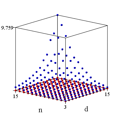
Figure 1: Timing comparison: OMF vs. Two-step approach

The horizontal axes correspond to $n$ and $d$ and the vertical axis corresponds to computing time $t$ in seconds. Each dot $(d,n,t)$ represents an experimental timing. The red dots indicate the experimental timing of the algorithm OMF, while the blue dots indicate the experimental timing of the two-step approach described above.

As can be seen, the algorithm OMF runs significantly more efficiently. This is due primarily to the cost of computing the Popov form of the last $n-1$ columns of the non-optimal moving frame. As described in [5], the complexity of this step is $O(d^{3}n^{7})$, which is bigger than $O(d^{2}n+d^{3}+n^{2})$, the complexity of the OMF (Proposition 38). Although other algorithms and implementations for Popov form computations may be more efficient than the one currently implemented in Maple, we still expect OMF to significantly outperform any similar two-step procedure, because the degree reduction step is essentially similar to a TOP reduced Gröbner basis computation for a module, which is computationally expensive.

7 Geometric interpretation and equivariance

In the introduction, we justified the term moving frame by picturing it as a coordinate system moving along a curve. This point of view is reminiscent of classical geometric frames, such as the Frenet-Serret frame. However, the frames in this paper were defined by suitable algebraic properties, not its geometric properties. It is then natural to ask if it is possible to combine algebraic properties of Definition 4 with some essential geometric properties, in particular with the group-equivariance property. In this section, we show that any deterministic algorithm for computing an optimal moving frame can be augmented to obtain an algorithm that computes a $GL_{n}(\mathbb{K})$-equivariant moving frame.

The group-equivariance property is essential for the majority of frames arising in differential geometry. For the Frenet-Serret frame it is manifested as follows. We recall that for a smooth curve $\gamma$ in $\mathbb{R}^{3}$, the Frenet-Serret frame at a point $p\in\gamma$ consists of the unit tangent vector $T$, the unit normal vector $N$ and the unit binormal vector $B$ to the curve at $p$. Consider the action of Euclidean group $E(3)$ (consisting of rotations, reflections, and translations) on $\mathbb{R}^{3}$. This action induces and action of the curves in $\mathbb{R}^{3}$ and on the vectors. It is easy to see that, for any $g\in E(3)$, the vectors $g\,T$, $g\,N$ and $g\,B$ are the unit tangent, the unit normal and the unit binormal, respectively, at the point $g\,p$ of the curve $g\,\gamma$. Thus, if we define $F_{\gamma}(p)=[T,N,P]$, then we can record the equivariance property as:

$$F_{g\,\gamma}(g\,p)=g\,F_{\gamma}(p)\quad\text{ for all }\gamma\subset\mathbb{R}^{3},p\in\gamma\text{ and }g\in E(3).$$ (30)

In the case of the algebraic moving frames considered in this paper, we are interested in developing an algorithm that for $\mathbf{a}\in\mathbb{K}[s]^{n}\backslash\{\bf 0\}$ produces an optimal moving frame $P_{\mathbf{a}}$ (recall Definition 4) with the additional $GL_{n}(\mathbb{K})$-equivariance property:

$$P_{\mathbf{a}\,g}(s)=g^{-1}\,P_{\mathbf{a}}(s)\text{ for all }\mathbf{a}\in\mathbb{K}[s]^{n}\backslash\{{\bf 0}\},s\in\mathbb{K}\text{ and }g\in GL_{n}(\mathbb{K}).$$ (31)

We observe that on the right-hand side of (30) the frame is multiplied by $g$, while on the right-hand side of (31) the frame is multiplied by $g^{-1}$. This means that the columns of $P$ comprise a right equivariant moving frame, while the Frenet-Serret frame is a left moving frame (see Definition 3.1 in [20] and the subsequent discussion).

To give a precise definition of a $GL_{n}(\mathbb{K})$-right-equivariant algebraic moving frame algorithm, consider the set $M=\mathbb{K}\times\left(\mathbb{K}[s]^{n}\backslash\{\bf 0\}\right)$, and view an algorithm producing an algebraic moving frame as a map $\rho\colon M\to GL_{n}(\mathbb{K})$ such that, for a fixed $\mathbf{a}$, the matrix $P_{\mathbf{a}}(s)=\rho(s,\mathbf{a})$ is polynomial in $s$ and satisfies Definition 4. Then the $GL_{n}(\mathbb{K})$-property (31) is equivalent to the commutativity of the following diagram:

On the top of the diagram, $L_{g}^{-1}$ indicates the right action of $g\in GL_{n}(\mathbb{K})$ on $GL_{n}(\mathbb{K})$ defined by multiplication from the left by $g^{-1}$, while on the bottom the right action is defined by $g\cdot(s,\mathbf{a})=(s,\mathbf{a}\,g)$.

We observe further that if the columns of $P$ comprise a right equivariant moving frame, then the rows of $P^{-1}$ comprise a left frame. The inverse algebraic frame has an easy geometric interpretation: the first row of $P^{-1}_{\mathbf{a}}$ equals to the position vector $\mathbf{a}$ and together with the last $n-1$ rows forms an $n$-dimensional parallelepiped whose volume does not change as the frame moves along the curve.

It is easy to find an instance of $g$ and $\mathbf{a}$ to show that $P_{\mathbf{a}}=OMF(\mathbf{a})$, where $OMF(\mathbf{a})$ is produced by Algorithm 1, does not satisfy (31) and, therefore, the OMF algorithm is not a $GL_{n}(\mathbb{K})$-equivariant algorithm. However, for input vectors $\mathbf{a}=[a_{1},\dots,a_{n}]$ such that $a_{1},\dots,a_{n}$ are independent over $\mathbb{K}$, the OMF algorithm can be augmented into a $GL_{n}(\mathbb{K})$-equivariant algorithm as follows:

Algorithm 2 (EOMF).

Input:

$\mathbf{a}=[a_{1},\dots,a_{n}]\not=0\in\mathbb{K}[s]^{n}$, row vector, where $n>1$, $\gcd(\mathbf{a})=1$, $\mathbb{K}$ a computable field, and components of $\mathbf{a}$ are linearly independent over $\mathbb{K}$.

Output:

$P\in\mathbb{K}[s]^{n\times n}$, a degree-optimal moving frame at $\mathbf{a}$

1. Construct an $n\times n$ invertible submatrix of the coefficient matrix of $\mathbf{a}$.

   1. $d\longleftarrow\deg(\mathbf{a})$

   2. Identify the row vectors $c_{0}=[c_{01},\dots c_{0n}],\ldots,c_{d}=[c_{d1},\dots c_{dn}]$ such that $\mathbf{a}=c_{0}+c_{1}s+\cdots+c_{d}s^{d}$.

   3. $I=[i_{1},\dots,i_{n}]\longleftarrow$ lexicographically smallest vector of integers between $0$ and $d$, such that vectors $c_{i_{1}},\dots,c_{i_{n}}$ are independent over $\mathbb{K}$.

   4. $\widehat{C}\longleftarrow\left[\begin{array}[]{c}c_{i_{1}}\\ \vdots\\ c_{i_{n}}\end{array}\right]$

2. Compute an optimal moving frame for a canonical representative of the $GL_{n}(\mathbb{K})$-orbit of $\mathbf{a}$.

   $$\widehat{P}\longleftarrow OMF(\mathbf{a}\,\widehat{C}^{-1})$$

3. Revise the moving frame $\widehat{P}$ so that the algorithm has the equivariant property (31).

   $$P\longleftarrow\widehat{C}^{-1}\widehat{P}.$$

To prove the algorithm we need the following proposition.

Proposition 40.

Let $P$ be a degree-optimal moving frame at a nonzero polynomial vector $\mathbf{a}$. Then, for any $g\in GL_{n}(\mathbb{K})$, the matrix $g^{-1}P$ is a degree-optimal moving frame at the vector $\mathbf{a}\,g$.

Proof.

By definition, $\mathbf{a}\,P=[\gcd(\mathbf{a}),0,\dots,0]$ and, therefore, for any $g\in GL_{n}(\mathbb{K})$ we have:

$$(\mathbf{a}\,g)\,g^{-1}P=[\gcd(\mathbf{a}),0,\dots,0].$$

From this, we conclude that $\gcd(\mathbf{a}\,g)=\gcd(\mathbf{a})$ and that $g^{-1}P$ is a moving frame at $\mathbf{a}\,g$. We note that the rows of the matrix $g^{-1}P$ are linear combinations over $\mathbb{K}$ of the rows of the matrix $P$. Therefore, the degrees of the columns of $g^{-1}P$ are less than or equal to the degrees of the corresponding columns of $P$.

Assume that $g^{-1}P$ is not a degree-optimal moving frame at $\mathbf{a}\,g$. Then there exists a moving frame $P^{\prime}$ at $\mathbf{a}\,g$ such that at least one of the columns of $P^{\prime}$, say the $j$-th column, has degree strictly less than the $j$-th column of $g^{-1}P$. Then, from the paragraph above, the $j$-th column of $P^{\prime}$ has degree strictly less than the degree of the $j$-th column of $P$.

By the same argument, $g\,P^{\prime}$ is a moving frame at $\mathbf{a}$ such that its $j$-th column has degree less than or equal to the degree of the $j$-th column of $P^{\prime}$, which is strictly less than the degree of the $j$-th column of $P$. This contradicts our assumption that $P$ is degree-optimal. ∎

Proof of the Algorithm 2. We first note that, since polynomials $a_{1},\dots,a_{n}$ are linearly independent over $\mathbb{K}$, then the coefficient matrix $C$ contains $n$ independent rows and, therefore, Step 1 of the algorithm can be accomplished. Let $\widehat{\mathbf{a}}=\mathbf{a}\,\widehat{C}^{-1}$, then $\mathbf{a}=\widehat{\mathbf{a}}\,\widehat{C}$ and $P$ is an optimal moving frame at $\mathbf{a}$ by Proposition 40. To show (31), for an arbitrary input $\mathbf{a}_{1}$ and an arbitrary $g\in GL_{n}(\mathbb{K})$, let $\mathbf{a}_{2}=\mathbf{a}_{1}\,g$. Then $\widehat{C}_{\mathbf{a}_{2}}=\widehat{C}_{\mathbf{a}_{1}}\,g$ and so

$$EOMF(\mathbf{a}_{2})=\widehat{C}_{\mathbf{a}_{2}}^{-1}OMF(\mathbf{a}_{2}\,\widehat{C}_{\mathbf{a}_{2}}^{-1})=g^{-1}\widehat{C}_{\mathbf{a}_{1}}^{-1}OMF(\mathbf{a}_{1}\,g\,g^{-1}\,\widehat{C}_{\mathbf{a}_{1}}^{-1})=g^{-1}\,EOMF(\mathbf{a}_{1}).$$

∎

Remark 41.

It is clear from the above proof that if, in Step 2 of Algorithm 2, we replace OMF with any (not necessarily degree-optimal) algorithm, then (not necessarily degree-optimal) frames produced by Algorithm 2 will have the $GL_{n}(\mathbb{K})$-equivariant property (31).

References

- [1] E. N. Antoniou, A. I. G. Vardulakis, and S. Vologiannidis. Numerical computation of minimal polynomial bases: a generalized resultant approach. Linear Algebra Appl., 405:264–278, 2005.
- [2] Felix Antritter and Jean Lévine. Flatness characterization: two approaches. In Advances in the theory of control, signals and systems with physical modeling, volume 407 of Lect. Notes Control Inf. Sci., pages 127–139. Springer, Berlin, 2010.
- [3] Bernhard Beckermann and George Labahn. Fraction-free computation of matrix rational interpolants and matrix GCDs. SIAM J. Matrix Anal. Appl., 22(1):114–144, 2000.
- [4] Bernhard Beckermann, George Labahn, and Gilles Villard. Shifted normal forms of polynomial matrices. In Proceedings of the 1999 International Symposium on Symbolic and Algebraic Computation (Vancouver, BC), pages 189–196. ACM, New York, 1999.
- [5] Bernhard Beckermann, George Labahn, and Gilles Villard. Normal forms for general polynomial matrices. J. Symbolic Comput., 41(6):708–737, 2006.
- [6] Theodorus Gertrudis Joseph Beelen. New algorithms for computing the Kronecker structure of a pencil with applications to systems and control theory. Technische Hogeschool Eindhoven, Department of Mathematics, Eindhoven, 1987. Dissertation, Technische Hogeschool Eindhoven, Eindhoven, 1987, With a Dutch summary.
- [7] Léandro Caniglia, Guillermo Cortiñas, Silvia Danón, Joos Heintz, Teresa Krick, and Pablo Solernó. Algorithmic aspects of Suslin’s proof of Serre’s conjecture. Comput. Complexity, 3(1):31–55, 1993.
- [8] Falai Chen, David Cox, and Yang Liu. The -basis and implicitization of a rational parametric surface. J. Symbolic Comput., 39(6):689–706, 2005.
- [9] Falai Chen and Wenping Wang. The -basis of a planar rational curve-properties and computation. Graphical Models, 64(6):368–381, 2002.
- [10] Howard Cheng and George Labahn. Output-sensitive modular algorithms for polynomial matrix normal forms. Journal of Symbolic Computation, 42:733 –750, 2007.
- [11] Jeanne N. Clelland. From Frenet to Cartan: the method of moving frames, volume 178 of Graduate Studies in Mathematics. American Mathematical Society, Providence, RI, 2017.
- [12] David A. Cox and Anthony A. Iarrobino. Strata of rational space curves. Comput. Aided Geom. Design, 32:50–68, 2015.
- [13] David A. Cox, Thomas W. Sederberg, and Falai Chen. The moving line ideal basis of planar rational curves. Comput. Aided Geom. Design, 15(8):803–827, 1998.
- [14] Carlos D’Andrea. On the structure of -classes. Comm. Algebra, 32(1):159–165, 2004.
- [15] Élie Cartan. La méthode du repère mobile, la théorie des groupes continus, et les espaces généralisés, volume 5 of Exposés de Géométrie. Hermann, Paris, 1935.
- [16] Mohamed Elkadi, André Galligo, and Thang Luu Ba. Approximate gcd of several univariate polynomials with small degree perturbations. Journal of Symbolic Computation, 47:410–421, 2012.
- [17] Anna Fabiańska and Alban Quadrat. Applications of the Quillen-Suslin theorem to multidimensional systems theory. In Gröbner bases in control theory and signal processing, volume 3 of Radon Ser. Comput. Appl. Math., pages 23–106. Walter de Gruyter, Berlin, 2007.
- [18] Rida T. Farouki. Rational rotation-minimizing frames—recent advances and open problems. Appl. Math. Comput., 272(part 1):80–91, 2016.
- [19] Rida T. Farouki, Carlotta Giannelli, Maria Lucia Sampoli, and Alessandra Sestini. Rotation-minimizing osculating frames. Comput. Aided Geom. Design, 31(1):27–42, 2014.
- [20] Mark Fels and Peter J. Olver. Moving Coframes. II. Regularization and Theoretical Foundations. Acta Appl. Math., 55:127–208, 1999.
- [21] Noaï Fitchas and André Galligo. Nullstellensatz effectif et conjecture de Serre (théorème de Quillen-Suslin) pour le calcul formel. Math. Nachr., 149:231–253, 1990.
- [22] Mark L. Green. The moving frame, differential invariants and rigidity theorems for curves in homogeneous spaces. Duke Math. Journal, 45:735–779, 1978.
- [23] Phillip A. Griffiths. On Cartan’s method of Lie groups as applied to uniqueness and existence questions in differential geometry. Duke Math. Journal, 41:775–814, 1974.
- [24] H. Guggenheimer. Computing frames along a trajectory. Comput. Aided Geom. Design, 6(1):77–78, 1989.
- [25] H. W. Guggenheimer. Differential Geometry. McGraw-Hill, New York, 1963.
- [26] Hoon Hong, Zachary Hough, and Irina A. Kogan. Algorithm for computing -bases of univariate polynomials. J. Symbolic Comput., 80(3):844–874, 2017.
- [27] Zachary Hough. -bases and algebraic moving frames: theory and computation. PhD thesis, 2018 (to be defended). http://www4.ncsu.edu/~zchough/.
- [28] Joe Imae, Yuki Akasawa, and Tomoaki Kobayashi. Practical computation of flat outputs for nonlinear control systems. In Proceedings of the 3rd International Conference on Manufacturing, Optimization, Industrial and Material Engineering (MOIME), IOP Conference Series-Materials Science and Engineering. IOP publishing, Bristol, 2015.
- [29] Thomas A. Ivey and Joseph M. Landsberg. Cartan for beginners: Differential geometry via moving frames and exterior differential systems, volume 175 of Graduate Studies in Mathematics. American Mathematical Society, Providence, RI, 2016.
- [30] Xiaohong Jia and Ron Goldman. -bases and singularities of rational planar curves. Comput. Aided Geom. Design, 26(9):970–988, 2009.
- [31] Alessandro Logar and Bernd Sturmfels. Algorithms for the Quillen-Suslin theorem. J. Algebra, 145(1):231–239, 1992.
- [32] Henri Lombardi and Ihsen Yengui. Suslin’s algorithms for reduction of unimodular rows. J. Symbolic Comput., 39(6):707–717, 2005.
- [33] Philippe Martin, Richard M. Murray, and Pierre Rouchon. Flat systems: open problems, infinite dimensional extension, symmetries and catalog. In Advances in the control of nonlinear systems (Murcia, 2000), volume 264 of Lect. Notes Control Inf. Sci., pages 33–57. Springer, London, 2001.
- [34] Peter Olver. Modern developments in the theory and applications of moving frames. In London Math. Soc. Impact150 Stories, volume 1, pages 14–50. London Math. Soc, 2015.
- [35] Hyungju Park and Cynthia Woodburn. An algorithmic proof of Suslin’s stability theorem for polynomial rings. J. Algebra, 178(1):277–298, 1995.
- [36] Jan W. Polderman and Jan C. Willems. Introduction to the Mathematical Theory of Systems and Control. Springer, New York, 1998.
- [37] Thomas Sederberg and Falai Chen. Implicitization using moving curves and surfaces. Computer Graphics Proceedings, Annual Conference Series, 2:301–308, 1995.
- [38] Ning Song and Ron Goldman. -bases for polynomial systems in one variable. Comput. Aided Geom. Design, 26(2):217–230, 2009.
- [39] Mohammed Tesemma and Haohao Wang. Intersections of rational parametrized plane curves. Eur. J. Pure Appl. Math., 7(2):191–200, 2014.
- [40] Bartel L. van der Waerden. Algebra I. Ungar, New York, 1970.
- [41] Antonis I. G. Vardulakis and Peter N. R. Stoyle. Generalized resultant theorem. J. Inst. Math. Appl., 22(3):331–335, 1978.
- [42] W. Wang, B. Jüttler, D. Zheng, and Y. Liu. Computation of rotation minimizing frame. ACM Trans. Graph, 27(1):18pp, 2008.
- [43] Jianmin Zheng and Thomas W. Sederberg. A direct approach to computing the -basis of planar rational curves. J. Symbolic Comput., 31(5):619–629, 2001.
- [44] Wei Zhou and George Labahn. Unimodular completion of polynomial matrices. In ISSAC 2014—Proceedings of the 39th International Symposium on Symbolic and Algebraic Computation, pages 413–420. ACM, New York, 2014.
- [45] Wei Zhou, George Labahn, and Arne Storjohann. Computing minimal nullspace bases. In ISSAC 2012—Proceedings of the 37th International Symposium on Symbolic and Algebraic Computation, pages 366–373. ACM, New York, 2012.