A new astrophysical solution to the Too Big To Fail problem

Abstract

Aims. We test whether or not realistic analysis techniques of advanced hydrodynamical simulations can alleviate the Too Big To Fail problem (TBTF) for late-type galaxies. TBTF states that isolated dwarf galaxy kinematics imply that dwarfs live in halos with lower mass than is expected in a $\Lambda$CDM universe. Furthermore, we want to identify the physical mechanisms that are responsible for this observed tension between theory and observations.

Methods. We use the moria suite of dwarf galaxy simulations to investigate whether observational effects are involved in TBTF for late-type field dwarf galaxies. To this end, we create synthetic radio data cubes of the simulated moria galaxies and analyse their H i kinematics as if they were real, observed galaxies.

Results. We find that for low-mass galaxies, the circular velocity profile inferred from spatially resolved H i kinematics often underestimates the true circular velocity profile, as derived directly from the enclosed mass. Fitting the H i kinematics of moria dwarfs with a theoretical halo profile results in a systematic underestimate of the mass of their host halos. We attribute this effect to the fact that the interstellar medium of a low-mass late-type dwarf is continuously stirred by supernova explosions into a vertically puffed-up, turbulent state to the extent that the rotation velocity of the gas is simply no longer a good tracer of the underlying gravitational force field. If this holds true for real dwarf galaxies as well, it implies that they inhabit more massive dark matter halos than would be inferred from their kinematics, solving TBTF for late-type field dwarf galaxies.

1 Introduction

Generally considered as the current standard model for cosmology and cosmic structure formation, $\Lambda$CDM is a superbly successful theory on large, super-galactic distance scales (Mamon et al. 2017; Rodríguez-Puebla et al. 2016; Planck Collaboration et al. 2016; Cai et al. 2014; Suzuki et al. 2012). However, towards smaller, sub-galactic scales, and especially in the regime of dwarf galaxies, $\Lambda$CDM encounters a number of persistent problems.

One such problem is referred to as Too Big Too Fail, or TBTF, first formulated in the context of the Local Group. Given the many factors that suppress star formation in dwarf galaxies, such as supernova feedback and the cosmic UV background, visible dwarf galaxies are expected to reside in relatively scarce high-$v_{\mathrm{circ}}$ dark-matter halos. This would also agree with their small observed number density. However, most observed Milky Way satellites have circular velocities $v_{\mathrm{circ}}<30\leavevmode\nobreak\ \mathrm{km\ s^{-1}}$, estimated from their stellar kinematics, indicating that these satellites seem to live in low-$v_{\mathrm{circ}}$ subhalos, which are too abundant in comparison with the observed number of Milky Way satellites (Boylan-Kolchin et al. 2011, 2012). The TBTF problem is also present for the satellite system of Andromeda (Tollerud et al. 2014) and for field dwarfs in the Local Group and Local Volume (e.g. Ferrero et al. 2012; Garrison-Kimmel et al. 2014; Papastergis et al. 2015).

Several possible solutions to this problem have been suggested. For example, if the Milky Way were to have a smaller virial mass, then it would also host a smaller number of massive subhalos (Wang et al. 2012). Another way out is to take into account the fact that baryonic processes, such as supernova feedback, can flatten the inner dark-matter density distribution, converting a high-$v_{\mathrm{circ}}$ cuspy density profile into a low-$v_{\mathrm{circ}}$ cored one at constant halo mass. By fitting the mass-dependent DC14 profile (Di Cintio et al. 2014) to the kinematical data of the Local Group dwarf galaxies, Brook & Di Cintio (2015a) found that dwarf galaxies inhabit more massive halos than previously thought, thus alleviating the TBTF problem. Other effects that help reduce dwarf galaxy circular velocities in the context of the Local Group include tidal stripping (Sawala et al. 2016b).

Papastergis & Shankar (2016, henceforth referred to as P16) discuss the TBTF in field dwarfs, where only internal baryonic effects can be invoked to reduce halo circular velocities. In their analysis, they use abundance matching to derive the relation between the observed H i rotation velocity inferred from the galaxy 21cm emission line profile, $W_{50}$, and the maximum halo circular velocity $v_{h,\mathrm{max}}$ such that the halo velocity function (VF) found in simulations (Sawala et al. 2015) corresponds to the observed field galaxy VF (Haynes et al. 2011; Klypin et al. 2015). Hereafter, we refer to this relation between $W_{50}$ and $v_{h,\mathrm{max}}$ as the P16 relation. Then, these authors fit NFW (Navarro et al. 1996) and DC14 profiles to the outer-most datapoint of the rotation curves of a set of field dwarf galaxies to infer their $v_{h,\mathrm{max}}$. This allows them to put individual $v_{\mathrm{rot},{H\textsc{I}}}-v_{h,\mathrm{max}}$ datapoints on the inferred statistical relation. As these authors note: “$\Lambda$CDM can be considered successful only if the position of individual galaxies on the $W_{50}-v_{h,\mathrm{max}}$ plane is consistent with the relation needed to reproduce the measured VF of galaxies.”. As it turns out, the individual galaxies are not consistent with the expected P16 relation.

The discrepancy between these results and those from Brook & Di Cintio (2015a) results from the radius at which the circular velocity is measured: For measurements beyond the core radius ($\gtrsim 2\mathrm{kpc}$), fitting a DC14 profile gives similar results to using a cusped NFW profile. The TBTF problem cannot, therefore, be (fully) explained by core creation alone (see also Papastergis & Ponomareva 2016).

For the present paper, we take to heart the message from P16: If $\Lambda$CDM is correct, then late-type field dwarfs should have higher circular velocities than is estimated from their H i kinematics. In order to investigate such a possible mismatch between the maximum circular velocity as inferred from gas kinematics and its actual value, we perform H i observations of a set of simulated dwarf galaxies. In Sect. 2, we briefly present the moria simulations and the procedure to construct and analyse mock H i data-cubes. In Sect. 3, we fit a halo profile to the outermost datapoint of the rotation curves of the simulated galaxies and compare with the results of P16. In Sect. 4 we give some possible explanations for these results. Our conclusions are presented in Sect. 5.

For clarity, we define the different types of velocities used throughout this paper here:

• $v_{\mathrm{rot,{H\textsc{i}}}}(R)$: the mean tangential velocity of the H i gas at a radius $R$ from the galaxy center. This can be determined from observations by fitting a tilted-ring model to the H i velocity field or the full data-cube.

• $v_{\mathrm{circ}}^{\mathrm{obs}}(R)$: the circular velocity derived from the $v_{\mathrm{rot,{H\textsc{i}}}}(R)$ profile by correcting for asymmetric drift (see Sect. 2.4).

• $v_{h}^{\mathrm{true}}(R)$: the “true” circular velocity profile, inferred from the total enclosed mass profile $M(R)$ as

  $$v_{h}^{\mathrm{true}}(R)=\sqrt{\frac{GM(R)}{R}}.$$ (1)

• $v_{\mathrm{out,{H\textsc{i}}}}=v_{\mathrm{circ}}^{\mathrm{obs}}(R_{\mathrm{out}})$: the outermost value of the rotation curve.

• $v_{h,\mathrm{max}}^{\mathrm{true}}=\mathrm{max}(v_{h}^{\mathrm{true}})$ : the maximum circular halo velocity.

• $v_{h,\mathrm{max}}^{\mathrm{fit}}$, $v_{h,\mathrm{max}}^{\mathrm{NFW}}$, or $v_{h,\mathrm{max}}^{\mathrm{DC14}}$: the maximum circular velocity obtained by fitting an NFW or DC14 profile to $v_{\mathrm{out,{H\textsc{i}}}}$. Denoted by $v_{h,\mathrm{max}}^{\mathrm{fit}}$ in general and $v_{h,\mathrm{max}}^{\mathrm{NFW}}$ or $v_{h,\mathrm{max}}^{\mathrm{DC14}}$ when the halo profile is specified.

• $W_{50}$ : the full width at half maximum (FWHM) of the galactic 21cm emission line profile, corrected for inclination to an edge-on view.

All, except for $W_{50}$ , refer to a spatially resolved kinematic measurement or calculation. $W_{50}$ on the other hand is derived from the spatially unresolved H i spectrum. Since $W_{50}$ does not correspond to any specific radius, it does not generally contain enough information to estimate the mass of the host halo by fitting a certain mass profile. However, $W_{50}$ measurements exist for large samples of galaxies, which allows for an accurate measurement of the number density of galaxies as a function of $W_{50}$, that is, the VF.

2 The MoRIA simulations

We use the moria (Models of Realistic dwarfs In Action) suite of $N$-body/SPH simulations of late-type isolated dwarf galaxies. These simulations are the result of letting isolated proto-galaxies, starting at $z=13.5$, merge over time along a cosmologically motivated merger tree (Cloet-Osselaer et al. 2014). The result is a galaxy with a relatively well constrained halo mass at $z=0$. This approach allows us to reach a resolution of $10^{3}-10^{4}\leavevmode\nobreak\ \mathrm{M}_{\odot}$ for the baryonic components and a force resolution of $5-15\leavevmode\nobreak\ \mathrm{pc}$, without being computationally too expensive. The resolution of dark matter particles is scaled with the cosmic baryon fraction $f_{\mathrm{bar}}=0.2115$, so that the number of baryonic and dark matter particles is the same.

The gas can cool radiatively and be heated by the cosmic UV background (De Rijcke et al. 2013). Once a gas parcel is dense enough, it is allowed to form stars. Stars inject energy in the interstellar medium (ISM) in the form of thermal feedback by young, massive stars and supernovae of types ia and type ii. The ISM absorbs 70% of the energy injected. A significant part of this energy is used to ionise the ISM (Vandenbroucke et al. 2013), which further decreases the effective energy coupling. To reduce excessive star formation at high redshift, we take the effects of Population iii stars into account. Stellar particles born out of extremely low-metallicity gas ($\mathrm{[Fe/H]}<-5$) are assumed to have a top-heavy IMF (Susa et al. 2014), resulting in earlier and stronger feedback (Heger & Woosley 2010). It is important to note that the atomic hydrogen density of every gas particle has already been computed, based on its density, temperature, composition, and incident radiation field, to be used in the subgrid model of the moria simulations, as described in De Rijcke et al. (2013). Thus, all H i observables we describe below are directly derived from the simulations without any extra assumptions or approximations. More details concerning the setup and subgrid physics model of these simulations can be found in Verbeke et al. (2015, V15), along with a demonstration of its validity.

Since this paper, more simulations were run with different masses and merger histories, but the conclusions presented in V15 still stand. At the moment of writing, moria consists of $\sim 30$ dwarf galaxy simulations, of which we discuss 10 in more detail. An overview of some of the basic properties of the 10 moria dwarfs discussed in this paper is presented in Table 1. M-1 to M-5 (M-6 to M-10) have a mass resolution of $4230\leavevmode\nobreak\ \mathrm{M}_{\odot}$ ($10515\leavevmode\nobreak\ \mathrm{M}_{\odot}$) for its baryonic component and a force resolution of $9.8\leavevmode\nobreak\ \mathrm{pc}$ ($13\leavevmode\nobreak\ \mathrm{pc}$).

(1)	(2)	(3)	(4)	(5)	(6)	(7)	(8)	(9)	(10)	(11)	(12)
Name	Symbol	$\log_{10}(M_{\star})$	$\log_{10}(M_{\mathrm{HI}})$	$\log_{10}(M_{200})$	$M_{V}$	$q$	$R_{\mathrm{out}}$	$v_{\mathrm{out},{H\textsc{i}}}$	$v_{h,\mathrm{max}}^{\mathrm{true}}$	$W_{50}/2$	$\sigma_{\star}$
		[$\mathrm{M}_{\odot}$]	[$\mathrm{M}_{\odot}$]	[$\mathrm{M}_{\odot}$]	[$\mathrm{mag}$]		[$\mathrm{kpc}$]	[$\mathrm{km\leavevmode\nobreak\ s^{-1}}$]	[$\mathrm{km\leavevmode\nobreak\ s^{-1}}$]	[$\mathrm{km\leavevmode\nobreak\ s^{-1}}$]	[$\mathrm{km\leavevmode\nobreak\ s^{-1}}$]
M-1	$\Diamond$	6.56	7.48	9.97	-12.35	0.49	1.68	21.66	36.16	14.30	10.84
M-2	$\star$	6.59	7.29	9.95	-12.52	0.63	1.21	39.87	36.43	24.35	18.51
M-3	$\Circle$	6.87	7.31	9.93	-12.77	0.74	1.13	19.45	33.81	15.00	12.95
M-4	$\bigtriangleup$	7.41	7.83	10.00	-13.92	0.41	2.37	17.04	37.60	18.58	12.55
M-5	$\bigtriangledown$	7.55	7.34	10.01	-14.35	0.53	1.09	41.69	43.10	41.53	18.89
M-6	$\triangleleft$	7.71	7.94	10.55	-14.93	0.76	1.93	39.04	52.72	27.02	21.60
M-7	$\triangleright$	8.00	8.49	10.41	-15.69	0.58	4.18	36.31	46.96	21.57	19.79
M-8	$\Square$	8.33	8.64	10.47	-16.50	0.61	4.87	45.79	54.49	29.33	26.49
M-9	$\pentagon$	8.53	8.59	10.42	-16.75	0.60	3.43	40.54	52.38	37.50	25.09
M-10	$\hexagon$	9.07	8.66	10.84	-18.17	0.56	4.15	53.94	67.30	38.27	33.94

Table 1: Properties of the 10 selected extscmo extscria simulations at $z=0$. (1) The name of the simulation, (2) the symbol used throughout the plots, (3) the stellar mass, (4) the H i mass, (5) the halo virial mass, (6) the total V-band magnitude, (7) the intrinsic flattening of the H i, (8) the H i radius, (9) the outermost value of the rotation curve, (10) the maximum circular velocity of the halo, (11) the half-width-half-max of the H i, and (12) the velocity dispersion of the stars at $R_{\mathrm{out}}$.

2.1 H i disk sizes and flattening

We aim to investigate H i rotation curves, with strong focus on the outer-most datapoint. It is therefore very important that the simulated dwarf galaxies have realistic H i disk sizes and shapes. In V15, we already showed that the moria dwarfs have an atomic interstellar medium (ISM) with realistic spatial substructure, as quantified by the H i power spectrum.

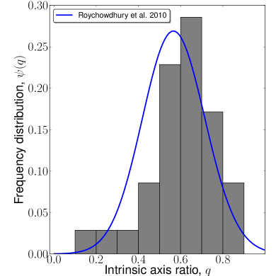
Figure 1: Histogram of the axis ratios of the moria dwarf galaxies versus the frequency distribution obtained by Roychowdhury et al. (2010) for the FIGGS galaxies.

Here, we also investigate the flattening and size of the H i disks. For this, we produce H i surface-density contour maps of the H i and fit ellipses to the contour corresponding to a column density of $\Sigma_{\mathrm{{H\textsc{i}}}}=1\ \mathrm{M_{\odot}}\ \mathrm{pc}^{-2}\approx 1.25\times 10^{20}m_{\mathrm{H}}\mathrm{cm}^{-2}$. We do this for different orientations and take the minimum value of the flattening $q$, defined as the ratio of the minor and major axis of the ellipse. In other words, $q$ is the intrinsic axis ratio of the galaxy. The frequency distribution of the axis ratio $q$ of the simulated moria galaxies is shown in Fig. 1, along with that of observed dwarf galaxies, derived by Roychowdhury et al. (2010) for the FIGSS sample of faint galaxies. In Fig. 2, we show the total H i mass, denoted by $M_{\mathrm{{H\textsc{i}}}}$, as a function of the disk size, $R_{\mathrm{out}}$, both for simulated and observed galaxies. The disk size is defined as the major axis of the elliptical contour corresponding to a column density of $\Sigma_{\mathrm{{H\textsc{i}}}}=1\ \mathrm{M_{\odot}}\ \mathrm{pc}^{-2}$.

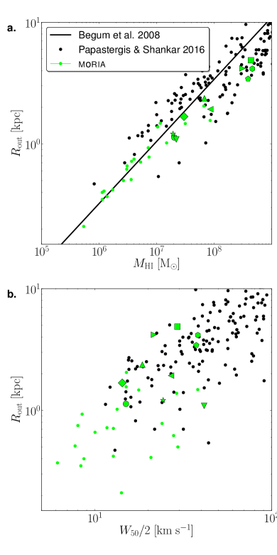
Figure 2: a. Atomic gas mass, $M_{\mathrm{{H\textsc{i}}}}$ versus H i disk size, $R_{\mathrm{out}}$, and b. $W_{50}/2$ versus $R_{\mathrm{out}}$ of the moria dwarfs (green, with symbols as indicated in Table 1. Green dots indicate simulations not in the Table.) versus observations compiled in P16 (in black). For the simulations, $R_{\mathrm{out}}$ is the semi-major axis of the best-fitted ellipse to the contour with $\Sigma_{\mathrm{{H\textsc{i}}}}=1\ \mathrm{M_{\odot}}\ \mathrm{pc}^{-2}$. The relation in panel a. is the one found for the FIGGS sample at $1\ \mathrm{M_{\odot}}\ \mathrm{pc}^{-2}$ ($\log(M_{\mathrm{{H\textsc{i}}}})=1.96\log(2R_{\mathrm{out}})+6.37$; Begum et al. 2008a).

We generally find good agreement with the observed flattening distribution, although the moria dwarfs appear to have slightly thicker H i disks than the observed dwarfs. However, the moria dwarfs were not intended to be equivalent to the FIGGS sample. Indeed, most of the FIGGS galaxies have $M_{\mathrm{{H\textsc{i}}}}\sim 10^{7}-10^{9}\mathrm{M_{\odot}}$ (Fig. 1c in Begum et al. 2008b) whereas more than half of the moria dwarfs lie in the $M_{\mathrm{{H\textsc{i}}}}\sim 10^{6}-10^{7}$ regime (see Fig. 2). Roychowdhury et al. (2010) also note that galaxies with high inclinations may be overrepresented in their sample which might lead to a slight underestimate for the mean intrinsic axis ratio $\langle q\rangle$. Furthermore, they assumed in their analysis that the gas disks are oblate spheroids, and showed that $\langle q\rangle$ would be higher when assuming a prolate spheroid. Galaxies are not necessarily oblate spheroids (e.g. Cloet-Osselaer et al. 2014), and therefore the real $\langle q\rangle$ might be higher. Considering these points, it is remarkable that we find a distribution that looks so similar to the observed one.

As can be seen in Fig. 2, the sizes of the H i disks of the moria dwarfs are also realistic; they follow the same mass-size relation and FWHM-size relation as the observed galaxies compiled in P16. This is of crucial importance because it determines the position of the outermost datapoint to which the circular velocity profile is fitted in order to estimate $v_{h,\mathrm{max}}^{\mathrm{fit}}$.

2.2 Mock data cubes

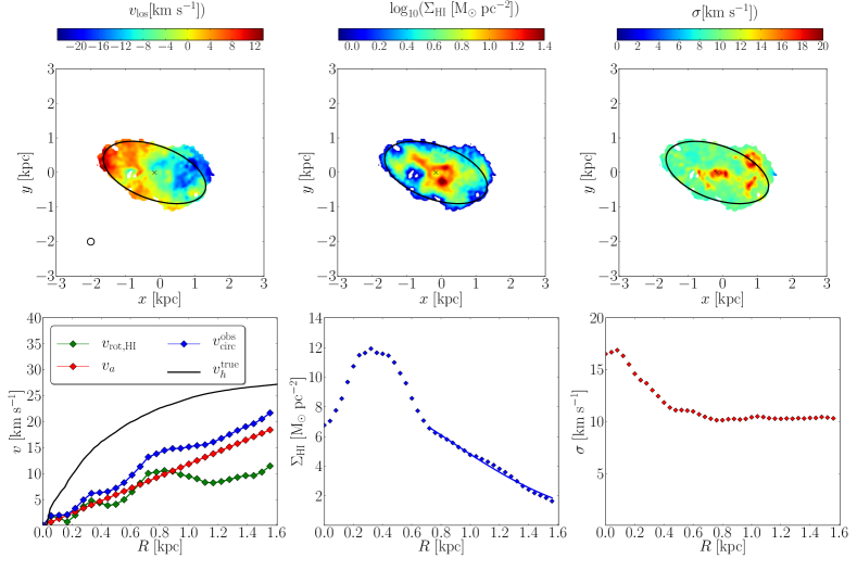
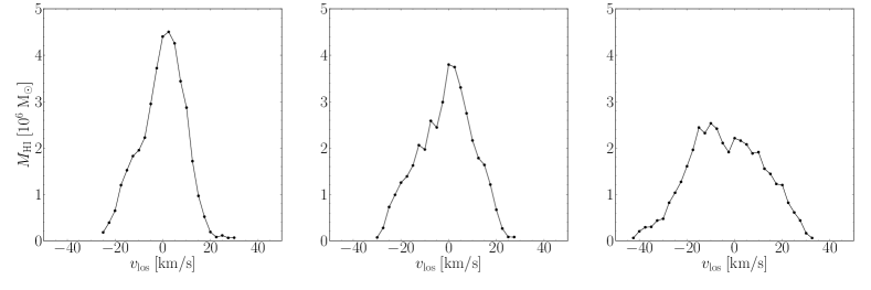
Figure 3: Top panels: velocity field (left), density (middle) and dispersion (right) map of M-1. The beam size used is shown in the top left panel. Middle panels: The rotation curves, with the rotational velocity obtained using tilted ring fitting in GIPSY in green, correction for pressure support in red, full circular velocity in blue and theoretical halo velocity in black (left), H i density profile, with the fit necessary for the pressure support correction plotted as a solid line shown over the area that was used for the fit (middle), H i velocity dispersion profile (right). Bottom panels: the global H i profile for the inclined view (left) as shown in the top panels and for two edge-on views (middle and right). The velocity bin width is the same as the channel width: $2.5\leavevmode\nobreak\ \mathrm{km\leavevmode\nobreak\ s^{-1}}$. The other moria galaxies are shown in Appendix A.

The procedure to produce a cube of 21cm data for a moria dwarf is as follows. First, we tilt the galaxy such that its angular momentum vector is inclined by 45^∘ with the line of sight. Then, the mass of each gas particle is assigned to a cell in a three-dimensional grid based on its projected position and its line-of-sight velocity. The velocity grid is chosen with a resolution of $2.5\ \mathrm{km\ s^{-1}}$. To account for thermal broadening, the H i mass of each gas particle is smeared out over neighbouring velocity channels using a Gaussian with a dispersion given by

$$\sigma_{\mathrm{TB}}=\sqrt{\frac{kT}{m_{p}}},$$ (2)

where $T$ is the temperature of the particle, $k$ is the Boltzmann constant, and $m_{p}$ is the proton mass. The gas is allowed to cool down to $T=10\ \mathrm{K}$ while it becomes fully ionised around $T\sim 10^{4}\ \mathrm{K}$. So the thermal broadening achieves values in the interval $0.29\ \mathrm{km\ s^{-1}}\lesssim\sigma_{\mathrm{TB}}\lesssim 10\ \mathrm{km\ s^{-1}}$. Finally, each velocity channel is convolved with a Gaussian beam profile as well. The FWHM of the beams are shown in the top-left panels in Figs. 3 and 11-19. The beam size was chosen so that it fits at least ten times within the H i radius of the galaxy. For the simulations presented here, this comes down to 100 pc for the ones with $R_{\mathrm{out}}\sim 1\ \mathrm{kpc}$ (M-1, M-2, M-3, M-5, and M-6) and $200\ \mathrm{pc}$ for the larger ones (M-4, M-7, M-8, M-9, and M-10). The resolution of the spatial grid is chosen so that the beam size corresponds to 5 pixels. The 3D mass grid is then saved in the FITS format.

2.3 Rotation curves

To achieve a realistic comparison analysis, we opt for two observational analysis codes to derive rotation curves for the moria dwarfs based on their radio data cubes: GIPSY (The Groningen Image Processing SYstem; van der Hulst et al. 1992) and ^3DBarolo (Di Teodoro & Fraternali 2015). GIPSY has a built-in routine, ROTCUR, which fits a tilted-ring model to the H i velocity field (Begeman 1989). Of the full suite of moria dwarfs, we selected ten with velocity fields and shapes that are sufficiently relaxed to be amenable to analysis with ROTCUR. The ones that were not selected had a very irregular H i morphology or velocity field due to their low masses. ^3DBarolo fits a model directly to the full data cube, which makes it useful for a comparison with the GIPSY results. The tilted-ring model in ^3DBarolo is populated with gas clouds at random spatial positions. This feature makes this code very useful for determining the kinematics of dwarf galaxies with sometimes highly disturbed gas distributions.

Ideally, given the way we produce the data cubes, one would expect the centre of each ring in the tilted-ring model to coincide with the nominal galaxy centre grid, its inclination to be $45^{\circ}$, and its position angle (PA) to be $90^{\circ}$. However, strongly disturbed and warped disks can lead to tilted-ring models with the apparent ring centres, inclinations, and PAs significantly shifted away from their expected values. The parameters are initially estimated by fitting an ellipse to the isodensity contour of $\Sigma_{\mathrm{{H\textsc{i}}}}=1\ \mathrm{M_{\odot}}\ \mathrm{pc}^{-2}$. These were checked and adjusted so that, for instance, the rotation would be around the minor axis. The inclination is typically fixed to its true value of $45^{\circ}$ (as determined by the position of the H i angular momentum vector). If the shape of the galaxy clearly implies a different inclination, we adjust it to better match this. The chosen ellipses are shown in the top panels of Figs. 3 and 11-19. The adjustment of the parameters will typically lead to a smaller maximal radius than $R_{\mathrm{out}}$. Also, the isodensity contours are not perfect ellipses (the chosen rings will thus go through areas with higher densities), leading to $\Sigma_{{H\textsc{\sc i}}}(R_{\mathrm{out}})>1\leavevmode\nobreak\ \mathrm{M_{\odot}}\ \mathrm{pc}^{-2}$. The systematic velocity is chosen as roughly the value of the centre (typically close to $0\ \mathrm{km\ s^{-1}}$). We keep these values fixed for each radius. The rotational velocity is thus the only parameter that is fitted.

2.4 Pressure support corrections

In the low-mass systems under investigation here, pressure support is expected to be significant, entailing a sizable correction. For the latter, we follow the approach typically used in observational studies of dwarf kinematics (e.g. Lelli et al. 2012). The pressure support correction is given by

$$v_{\mathrm{a}}^{2}(R)=-\sigma^{2}\frac{\partial\ln(\sigma^{2}\Sigma_{\mathrm{{H\textsc{i}}}})}{\partial\ln R},$$ (3)

where $\sigma$ is the velocity dispersion and $\Sigma_{\mathrm{{H\textsc{i}}}}$ is the intrinsic gas surface-density. We assume a prescription for $\Sigma_{\mathrm{{H\textsc{i}}}}$ of the form

$$\Sigma_{\mathrm{{H\textsc{i}}}}(R)=\Sigma_{0}\exp(-R^{2}/2s^{2}),$$ (4)

with $s$ being a radial scale length. Since we are only interested in $v_{\mathrm{out}}$, the fit is performed for the outer regions and the velocity dispersion is assumed constant at the value at the outer edge of the galaxy. This is justified since the radial variation of $\sigma$ is typically small. The pressure support correction then becomes

$$v_{\mathrm{a}}^{2}(R)=\sigma_{\mathrm{out}}^{2}\frac{R^{2}}{s^{2}}.$$ (5)

We also tried other commonly used prescriptions for $\Sigma_{\mathrm{{H\textsc{\sc i}}}}$, as well as for $\sigma^{2}\Sigma_{\mathrm{{H\textsc{\sc i}}}}$ (e.g. Oh et al. 2015). This lead to the same general results. Given the rotation velocity $v_{\mathrm{rot}}$ provided by the tilted-ring fit and the pressure support correction $v_{\mathrm{a}}$, we obtain an estimate for the true circular velocity as

$$v_{\mathrm{circ}}^{\mathrm{obs}}(R)=\sqrt{v_{\mathrm{rot,{H\textsc{i}}}}^{2}(R)+v_{\mathrm{a}}^{2}(R)}.$$ (6)

The obtained rotation curves are shown in the middle left panels of Figs. 3 and 11-19. In these Figs. we show the three first moment maps of the data cube, the rotation and circular velocity curves, the radial H i density profile, and the H i velocity dispersion profile. In the density profile diagram, the region where the parameters of the pressure support model have been determined is indicated. In this region, the pressure support correction can be computed relatively reliably; at smaller radii, the resulting pressure support correction may not be as reliable.

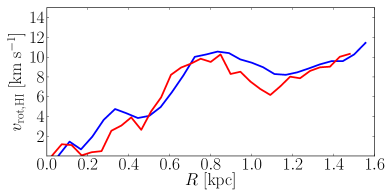
Figure 4: Rotation curves of M-1, obtained using GIPSY (in blue) and using ^3DBarolo (in red).

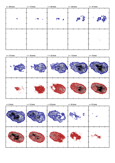
Figure 5: Channel maps of M-1, in blue, and the model fit with ^3DBarolo, in red. The ^3DBarolo model reproduces the most salient features of the input data cubes.

In Fig. 4, we compare rotation curves determined with GIPSY and with ^3DBarolo. For the tilted-ring analysis with ^3DBarolo, we used 20 rings, each with a radial size of $10\leavevmode\nobreak\ \mathrm{arcsec}\approx 50\leavevmode\nobreak\ \mathrm{pc}$. We keep all parameters the same as in the analysis with GIPSY while fitting the rotational velocity, with the exception of an additional free parameter of scale height. We notice from the channel maps, two of which are shown in Fig. 5, that our observed simulations (in blue) and the model (in red) agree relatively well. Overall, the agreement between the results obtained with both codes is satisfactory, especially in the outer regions that are of greatest interest to us.

We note that, since we have focused on obtaining the rotation curves and pressure support corrections in the outer regions, we do not make strong claims about the rotation in the central regions. To investigate, for example, the universality of dwarf galaxy rotation curves (Karukes & Salucci 2017) or the radial acceleration relation (McGaugh et al. 2016; Lelli et al. 2017) for the moria galaxies, we would need to realistically obtain rotation curves at all radii. This lies beyond the scope of this paper.

3 Results

3.1 The $W_{50}-v_{\mathrm{out},{H\textsc{\sc i}}}$ relation

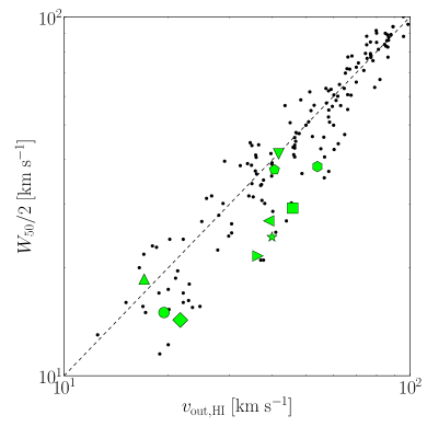
Figure 6: $W_{50}/2$ versus $v_{\mathrm{out},{H\textsc{\sc i}}}$ for the moria dwarfs. Symbols are as indicated in Table 1. Observations, compiled in P16, are shown in black. The dashed lines show the case for both quantities being equal.

An often-posed question is how $W_{50}$, which is relatively easy to measure, relates to the harder-to-obtain $v_{\mathrm{out},{H\textsc{\sc i}}}$ (see e.g. Brook & Shankar 2016; Ponomareva et al. 2016). Fig. 6 shows the relation between the two quantities for observed low-mass galaxies (compiled in P16). For galaxies with $v_{\mathrm{out},{H\textsc{\sc i}}}\lesssim 70\leavevmode\nobreak\ \mathrm{km\leavevmode\nobreak\ s^{-1}}$, the scatter on the relation becomes significant, and it typically holds that $W_{50}/2<v_{\mathrm{out},{H\textsc{\sc i}}}$. The moria galaxies follow the trend of the observations, although some seem to be on the low-end of the data.

3.2 The $W_{50}-v_{h,\mathrm{max}}$ relation

In their study of the TBTF problem in field dwarfs, P16 derived the average relation between the observed H i velocity width of galaxies, $W_{50}$, and the maximum circular velocity of their host halos, $v_{h,\mathrm{max}}^{\mathrm{true}}$, such that the observed VF of galaxies (Haynes et al. 2011; Klypin et al. 2015) can be reproduced within the $\Lambda$CDM cosmological model. The observed rotation velocity we use here is $W_{50}/2$.

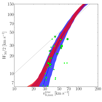
Figure 7: The moria dwarfs in the $W_{50}-v_{h,\mathrm{max}}$ plane. Green symbols are the simulations for which resolved rotation curves are available, with their symbols as indicated in Table 1. Green dots indicate moria simulations not explicitly discussed. The red and blue lines are the P16 relations derived from different observational datasets, with the bands around them representing their uncertainty.

Figure 7 shows the location of the moria dwarfs in the $W_{50}-v_{h,\mathrm{max}}^{\mathrm{true}}$ plane. The moria dwarfs follow the average relation derived in P16 very well, a fact that ensures that moria dwarfs are produced at the correct number densities as a function of their $W_{50}$ (i.e. the moria simulation reproduces the observational VF). Similar results were also obtained by Macciò et al. (2016) based on the NIHAO hydrodynamical simulations (Wang et al. 2015) and by Brooks et al. (2017) based on a set of hydrodynamic simulations of galaxy formation carried out by Governato et al. (2012), Brooks & Zolotov (2014) and Christensen et al. (2014).

However, reproducing the observational VF alone does not necessarily mean that the cosmological problems faced by $\Lambda$CDM on small scales have been resolved. In particular, a successful simulation must also be able to reproduce the internal, spatially resolved kinematics of observed dwarfs. This is a crucial point, since the inconsistency between the predicted velocity profiles of simulations that are able to reproduce the observational VF, and the measured outermost-point rotational velocities of small dwarfs is at the heart of the TBTF problem (e.g. Papastergis & Ponomareva 2016, see also Trujillo-Gomez et al. 2016; Schneider et al. 2016).

3.3 Halo profile fitting

The NFW profile (Navarro et al. 1996) has the form

$$\rho_{\mathrm{NFW}}(R)=\frac{\rho_{s}}{\left(\frac{R}{R_{s}}\right)\left(1+\frac{R}{R_{s}}\right)^{2}},$$ (7)

and the DC14 profile is given by the expression (Di Cintio et al. 2014)

$$\rho_{\mathrm{DC14}}(R)=\frac{\rho_{s}}{\left(\frac{R}{R_{s}}\right)^{\gamma}\left(1+\left(\frac{R}{R_{s}}\right)^{\alpha}\right)^{(\beta-\gamma)/\alpha}},$$ (8)

where $R_{s}$ is scale length and $\rho_{s}$ is a multiple of the density at radius $R=R_{S}$. The NFW profile was derived from dark-matter-only simulations while the DC14 profile takes the halo response to baryonic effects into account. The $\alpha$, $\beta$, and $\gamma$ parameters are set by the star formation efficiency of the galaxy (quantified by the ratio of stellar to halo mass, $M_{\star}/M_{h}$). For $\alpha=1$, $\beta=3$, and $\gamma=1$, the DC14 profile coincides with the NFW profile. If the stellar mass of the galaxy is known, both profiles have only two free parameters: the halo mass $M_{h}$ and the halo concentration $c=R_{\mathrm{vir}}/R_{s}$, with $R_{\mathrm{vir}}$ , the virial radius.

P16 fitted both these profiles to the velocity measured at the outermost H i point of each galaxy (data taken from Begum et al. (2008a); de Blok et al. (2008); Oh et al. (2011); Swaters et al. (2009, 2011); Trachternach et al. (2009); Kirby et al. (2012); Côté et al. (2000); Verheijen & Sancisi (2001); Sanders (1996); Hunter et al. (2012); Oh et al. (2015); Cannon et al. (2011); Giovanelli et al. (2013); Bernstein-Cooper et al. (2014)). They fixed the halo concentration to the mean cosmic value ($\log_{10}c=0.905-0.101\log_{10}(M_{h}/(10^{12}h^{-1}\mathrm{M_{\odot}}))$; Dutton & Macciò 2014), leaving only the halo mass as a free parameter. From the fitted profile, they compute the maximum circular velocity of each galaxy’s host halo. In a successful cosmological model, individual galaxies should have $W_{50}-v_{h,\mathrm{max}}^{\mathrm{fit}}$ data-points that agree with the average $W_{50}-v_{h,\mathrm{max}}^{\mathrm{true}}$ relation that is needed to reproduce the observed VF (blue and red bands in Fig. 7). As shown by P16, all is not well; a sizable fraction of low-mass galaxies fall to the left of the expected $W_{50}-v_{h,\mathrm{max}}^{\mathrm{true}}$ relation. In other words, the halo circular velocity implied by their H i kinematics is too low.

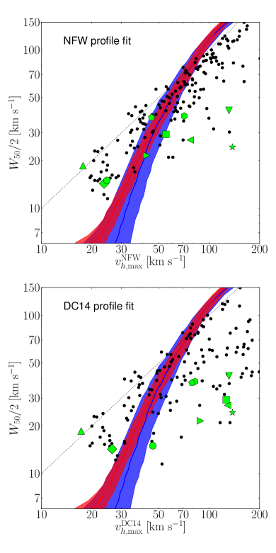
Figure 8: Results from fitting a NFW (top panel) and DC14 (bottom panel) to the outer-most point of the rotation curves of the moria simulations using a fixed halo concentration (symbols as indicated in Table 1). This is compared to the results from P16 (in black). Red and blue lines and bands are the same as in Fig. 7.

We exactly replicate this analysis for the moria dwarfs and show the results in Fig. 8. Although there are fewer moria dwarfs than in the P16 sample, the result is broadly the same: the $W_{50}-v_{h,\mathrm{max}}^{\mathrm{fit}}$ relation is inconsistent with the expected $W_{50}-v_{h,\mathrm{max}}^{\mathrm{true}}$ relation. The simulations with the highest $v_{h,\mathrm{max}}^{\mathrm{fit}}$-values seem to lie on the low end of, or even slightly below, the datapoints. This can be attributed to their lower-than-average $W_{50}$-values (see Fig. 6). Another explanation is their smaller-than-average $R_{\mathrm{out}}$ values (see Fig. 2a), since for smaller radii, the uncertainties on $v_{\mathrm{out,{H\textsc{\sc i}}}}$ will be extrapolated to large uncertainties on $v_{h,\mathrm{max}}^{\mathrm{fit}}$. The two (low $W_{50}$ and small $R_{\mathrm{out}}$ values) most likely work together and probably come hand-in-hand. Indeed, for smaller H i bodies, the potential will be traced at smaller radii, resulting in a lower $W_{50}$.

Analysed in this way, one would be driven to the conclusion that the moria dwarfs do not follow the $W_{50}-v_{h,\mathrm{max}}^{\mathrm{true}}$ relation required for the $\Lambda$CDM halo VF to match the observed galactic VF and, therefore, that they suffer from the TBTF problem. The crucial difference between Figs. 7 and 8 is the fact that in the former, the maximum halo velocity, $v_{h,\mathrm{max}}^{\mathrm{true}}$, is computed directly from the enclosed mass profile of each simulated galaxy, while in the latter, $v_{h,\mathrm{max}}^{\mathrm{fit}}$ is computed by fitting the mock H i kinematics of each simulated galaxy.

4 Discussion

4.1 Does the H i rotation curve trace the potential?

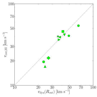
Figure 9: The measured H i rotation at $R_{\mathrm{out}}$ compared to the dynamical circular velocity, as expected from the enclosed mass. Symbols are as indicated in Table 1.

The fact that $v_{h,\mathrm{max}}^{\mathrm{true}}$ and $v_{h,\mathrm{max}}^{\mathrm{fit}}$ have different values might be explained by an observational effect: The H i rotation curve of dwarf galaxies does not exactly follow the underlying potential.

Indeed, as one can see in Fig. 9, the H i circular velocity profiles ($v_{\mathrm{circ}}^{\mathrm{obs}}(R)$) of the moria dwarfs are quite different from the true circular velocity profiles ($v_{h}^{\mathrm{true}}(R)$), even after correcting for pressure support. More often than not, the outer H i rotation velocity data-point falls significantly below the true value of the local circular velocity. It is important to keep in mind that the preceding statement is not directly related to the fact that rotational velocities derived from the linewidth of the HI profile of dwarf galaxies, $W_{50}/2$, underestimate the maximum circular velocity of the host halo, $v_{h,\mathrm{max}}^{\mathrm{true}}$, a result that has already been reported by Macciò et al. (2016) and Brooks et al. (2017). In fact, the linewidth-derived H i velocity probes radii much smaller than the radius where the host halo rotation curves peak, and thus there is no guarantee that the two quantities should be the same. Further more, this is different from the fact that the H i rotation curve is still rising at its outer-most radius and thus does not trace $v_{h,\mathrm{max}}^{\mathrm{true}}$ (Brook & Di Cintio 2015b; Ponomareva et al. 2016). What we demonstrate here instead is that the circular velocity computed from spatially resolved H i data underestimates the true circular velocity at the same radius. Of course, there are only ten moria dwarf galaxies with resolved rotation curves and a bigger sample of simulated dwarfs is definitely required to fully explore this issue. But if this explanation holds water, it would explain why the halo fitting using a fixed concentration fails; we are not fitting to the actual halo velocity at this radius.

In Appendix B, we briefly redo the halo fitting, but now fixing the halo mass using an abundance-matching relation and keeping the halo concentration as a free parameter. In short, the resulting concentrations do not seem to be drawn from the distribution predicted by $\Lambda$CDM, especially for galaxies with low $W_{50}$. If the observed H i rotation curve does not trace the potential, this would explain the seemingly incorrect population of concentrations.

Valenzuela et al. (2007) and Pineda et al. (2017) have also applied a tilted-ring method to derive the H i rotation curve to investigate whether dwarf galaxies have dark matter cusps or cores. They studied galaxies with an idealised set-up and both find that the observed H i rotation underestimates the gravitational potential; only in the inner regions, however. Here, using more realistic dwarf galaxies, we show that the idea that the H i rotation is not necessarily a good tracer for the underlying gravitational potential of dwarf galaxies is not necessarily confined to the inner regions of galaxies, but extends over their entire body.

One crucial question here is what causes this substantial underestimate of the local circular velocity in observational measurements of the HI kinematics. We attribute this to the fact that the assumptions underlying the tilted-ring fitting method and the correction for pressure support are not met in the case of low-mass dwarf galaxies; their atomic ISM simply does not form a relatively flat, dynamically cold disc. Rather, they have a vertically thick ($\langle q\rangle\sim 0.5$), dynamically hot, continuously stirred atomic ISM with significant substructures, that is not in dynamical equilibrium in the gravitational potential. The detailed analysis of the vertical structure of the HI disks of moria dwarfs and of non-circular motions in their velocity fields will be the focus of a separate publication (Verbeke et al. in prep.)

4.2 Stellar kinematics

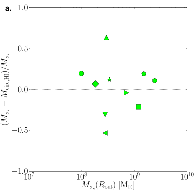
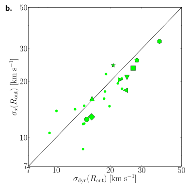
Figure 10: a. The relative difference between the enclosed mass within $R_{\mathrm{out}}$ inferred from stellar velocity dispersions $\sigma_{\star}$ and H i circular motions. b. The stellar velocity dispersion within $R_{\mathrm{out}}$ compared to the dynamical velocity dispersion, as expected from the enclosed mass. Symbols are as indicated in Table 1, with dots representing the moria galaxies without resolved rotation curves.

In accordance with the analysis of P16, we have used H i ordered motions to get an idea of the underlying gravitational potential. Late-type dwarf galaxies are typically dispersion-supported (Kirby et al. 2014; Wheeler et al. 2017). So the stellar velocity dispersion $\sigma_{\star}$ of a late-type dwarf can also be used to obtain a mass estimate, by using

$$M_{\sigma_{\star}}(R)=3\sigma_{\star}^{2}RG^{-1}.$$ (9)

For our simulations, we want to calculate $\sigma_{\star}$ in the same way as is done observationally (Kirby et al. 2014). In the same vein as Vandenbroucke et al. (2016), we weigh the average with the number of red giant branch (RGB) stars expected in each stellar particle (using the stellar evolution models of Bertelli et al. 2008, 2009). As shown in Fig. 10a, the enclosed mass within $R_{\mathrm{out}}$ inferred from the stellar velocity dispersion agrees reasonably well with the one inferred from the H i kinematics ($M_{\mathrm{circ,{H\textsc{\sc i}}}}=v_{\mathrm{out,{H\textsc{\sc i}}}}^{2}R_{\mathrm{out}}G^{-1}$). The mass estimated from stellar velocity dispersions agrees typically within $\sim 30\%$ with the mass inferred from the HI rotation curve. Two simulations however have a relative difference of $\sim 50\%$.

Fig. 10b shows the measured stellar velocity dispersion within $R_{\mathrm{out}}$ as a function of the dynamical one, $\sigma_{\mathrm{dyn}}$, as expected from the enclosed mass. We note that we have only included simulations with at least 100 stellar particles within $R_{\mathrm{out}}$, to get a good measure of $\sigma_{\star}$. Contrary to Fig. 9, the lowest-mass moria dwarfs do not systematically have lower observed stellar velocity dispersions than dynamical ones. However, over our entire sample, the majority of the simulated dwarfs have $\sigma_{\star}<\sigma_{\mathrm{dyn}}$. This implies that in most cases, their dynamical mass would be underestimated from observed stellar kinematics.

Given this, the results presented in this paper might also be extended to the TBTF problem for satellite galaxies. However, other effects play an important role. The presence of H i and active star formation (and thus stellar feedback) in field dwarfs will influence the stellar kinematics through dynamical heating or cooling. Satellites are devoid of H i but will, on the other hand, be influenced by the tidal field from their host galaxy. A similar study of simulated satellite galaxies is thus necessary to see if their stellar kinematics underestimate the halo mass.

4.3 Are disturbed velocity fields realistic?

As can be seen from Figs. 11-19, the H i distributions of the moria galaxies are generally quite disturbed. This is also the case for most real dwarf galaxies with velocity widths $W_{50}/2\lesssim 30\ \mathrm{km\leavevmode\nobreak\ s^{-1}}$; see e.g. Leo P (Bernstein-Cooper et al. 2014), CVndwA, DDO 210, and DDO 216 (Oh et al. 2015). However, galaxies with larger velocity widths, $W_{50}/2\sim 40-70\mathrm{km\leavevmode\nobreak\ s^{-1}}$, typically display regular velocity fields and low H i velocity dispersions, $\sigma_{\mathrm{{H\textsc{i}}}}\lesssim 12\mathrm{km\leavevmode\nobreak\ s^{-1}}$ (e.g. Kirby et al. 2012; Iorio et al. 2017). In contrast, the most massive moria dwarf that we have analysed, M-10, has a fairly disturbed velocity field and a relatively large velocity dispersion, $\sigma_{\mathrm{{H\textsc{i}}}}\gtrsim 20\mathrm{km\leavevmode\nobreak\ s^{-1}}$ (see Fig. 19). Even though we cannot draw reliable conclusions from this one object alone, it is possible that this indicates that the efficiency of stellar feedback in the moria simulation is too strong. We note that most state-of-the-art hydrodynamic simulations of dwarf galaxy formation (e.g. Hopkins et al. 2014; Wang et al. 2015; Sawala et al. 2016a) have more efficient feedback schemes than moria, so this could represent a general issue for (dwarf) galaxy simulations. At the same time however, the moria simulation succesfully reproduces the sizes and thicknesses of H i disks of observed dwarfs (Figs. 1 2). Moreover, in Fig. 9 of V15 we show that the spatial distribution of H i in moria dwarfs has similar power spectrum slopes as those measured for LITTLE THINGS galaxies (Zhang et al. 2012; Hunter et al. 2012). We leave the investigation of this, including, for example, the effect of beam size, for future research.

In any case, this does not change the conclusions of this paper in any way, since these are based on the galaxies with $W_{50}/2\lesssim 30\ \mathrm{km\leavevmode\nobreak\ s^{-1}}$.

5 Conclusions

We have used the moria simulations of dwarf galaxies with realistic H i distributions and kinematics to investigate the Too Big To Fail problem for late-type field dwarfs.

We showed that the moria dwarfs follow the relation between H i line-width and halo circular velocity, derived by Papastergis & Shankar (2016), which is required for the $\Lambda$CDM halo velocity function to correspond to the observed field galaxy width function. This means that, given the number density of halos formed in a $\Lambda$CDM universe, the moria simulations reproduce the observed galactic velocity function. In other words: there are no missing dwarfs in the moria simulations.

We then constructed resolved H i rotation curves, including corrections for pressure support, for ten of the moria dwarf galaxies. We used our mock H i rotation curves to replicate the analysis of Papastergis & Shankar (2016) and fitted NFW and DC14 density profiles (with fixed concentration parameter) to the outermost point of these measured rotation curves to derive an observational estimate for the maximum halo circular velocity of each moria galaxy. Using this estimate for the circular velocity, the moria dwarfs, like the real dwarf galaxies analysed by Papastergis & Shankar (2016), fail to adhere to the relation between H i line-width and halo circular velocity that is required for the $\Lambda$CDM halo velocity function to correspond to the observed field galaxy width function. In other words, using only quantities derived from observations, dwarf galaxies (both real and simulated) experience the TBTF problem. What causes this difference between the results from fitting a halo profile to the outer-most point of the rotation curve and using the actual $v_{h,\mathrm{max}}^{\mathrm{true}}$-value derived directly from the mass distribution?

Comparing the H i rotation curves of the moria dwarf galaxies with their theoretical halo circular velocity curves, we see that they can differ significantly. The circular velocities derived from the H i kinematics of moria dwarfs with H i rotation velocities below $\sim 30\ \mathrm{km\ s^{-1}}$ are typically too low. This results in a $v_{h,\mathrm{max}}^{\mathrm{fit}}$ value that is too low at a fixed concentration $c$. The TBTF problem thus results, at least partially, from the fact that for galaxies in this regime, their halo mass cannot readily be inferred from their (H i) kinematics. Indeed, based on their kinematics, galaxies with $W_{50}/2\lesssim 30\ \mathrm{km\ s^{-1}}$ are predicted to inhabit halos that are less massive than observations would suggest. However, under the assumptions of $\Lambda$CDM, the P16 relation does provide an estimate of the true halo circular velocity $v_{h,\mathrm{max}}^{\mathrm{true}}$ as a function of a galaxy’s H i linewidth $W_{50}$.

We attribute this effect to that fact that the atomic interstellar medium of low-mass dwarfs simply does not form a relatively flat, dynamically cold disc whose kinematics directly trace the underlying gravitational force field. Another explanation might be that the H i velocity fields are too irregular to infer halo mass from kinematics. This is true for most of the simulated galaxies presented in this work, as well as for observed low-mass galaxies.

The stellar feedback efficiency will influence both the H i-thickness of the galaxies, as well as how messy the velocity fields are. Thus, how much energy is actually injected in the ISM by stellar feedback is an important issue in the discussion of the TBTF problem.

Appendix A H i catalogue

A synthetic observation of one our simulations was already presented in Fig. 3. Here, the rest of the moria simulations discussed in this paper are shown.

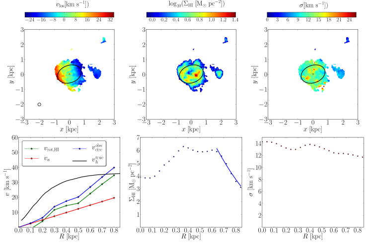
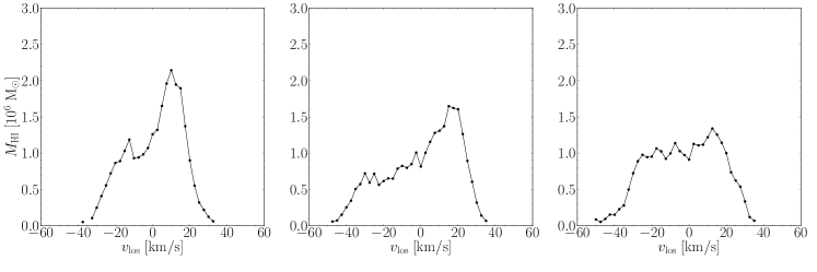
Figure 11: Same as in Fig. 3, but for M-2.

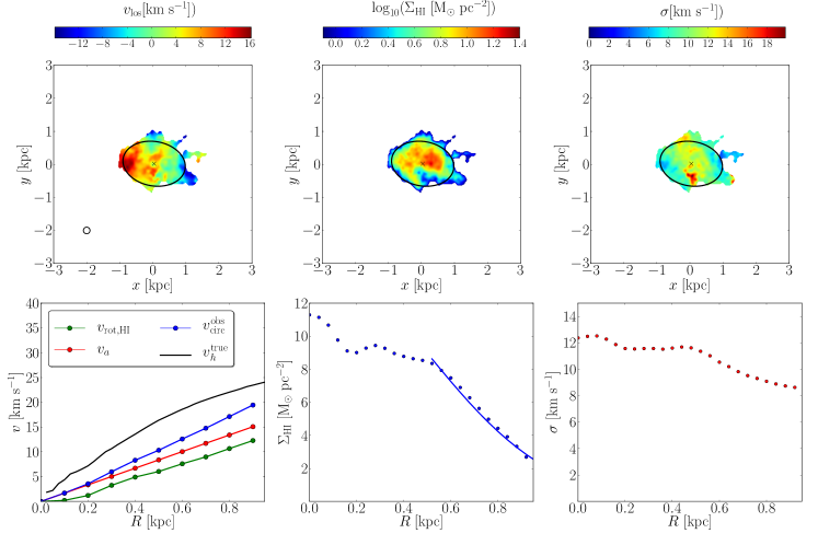
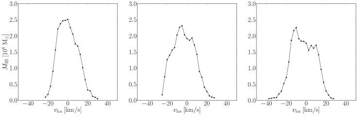
Figure 12: Same as in Fig. 3, but for M-3.

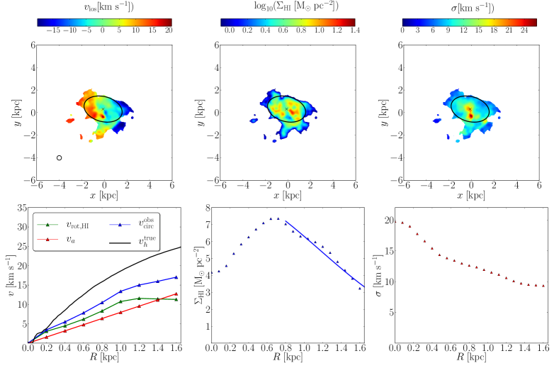
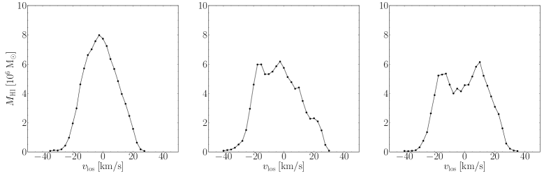
Figure 13: Same as in Fig. 3, but for M-4.

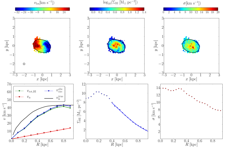
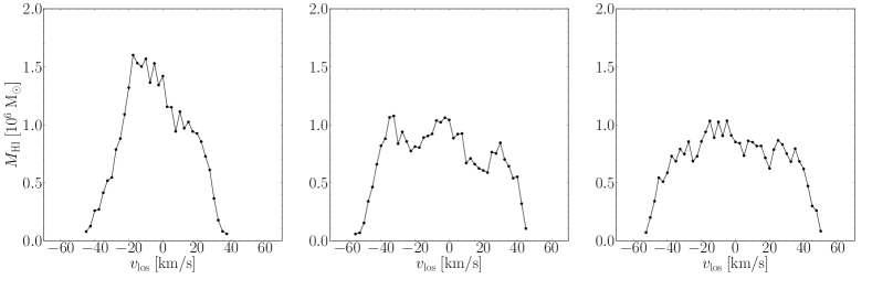
Figure 14: Same as in Fig. 3, but for M-5.

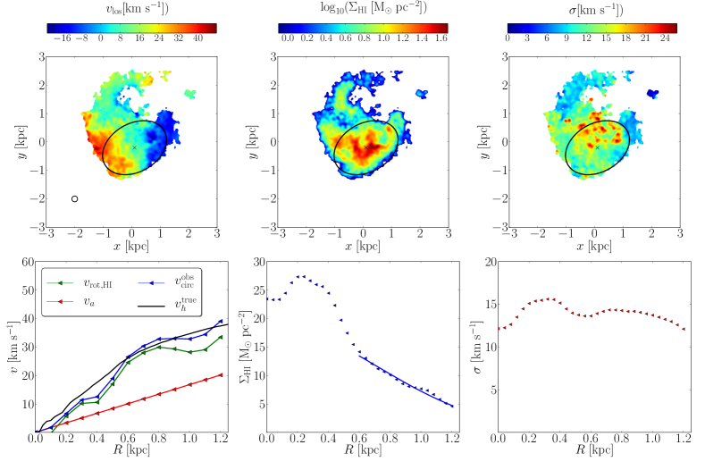
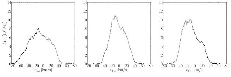
Figure 15: Same as in Fig. 3, but for M-6.

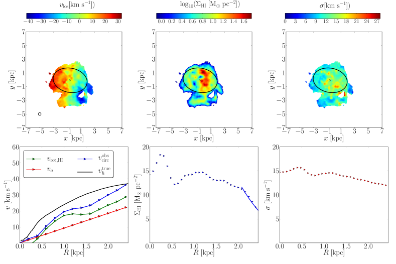
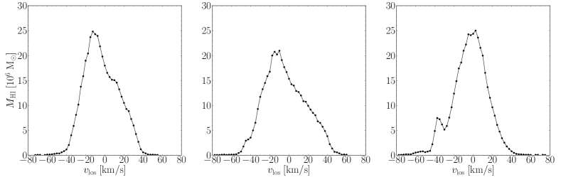
Figure 16: Same as in Fig. 3, but for M-7.

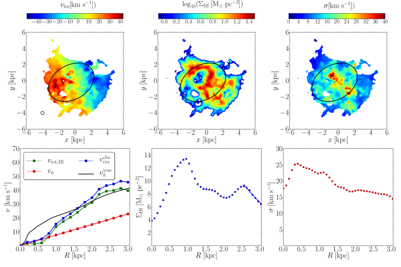
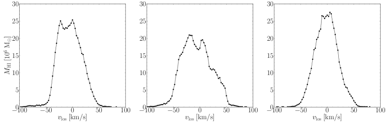
Figure 17: Same as in Fig. 3, but for M-8.

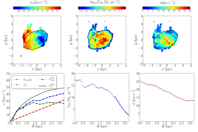
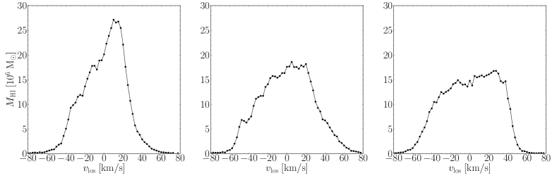
Figure 18: Same as in Fig. 3, but for M-9.

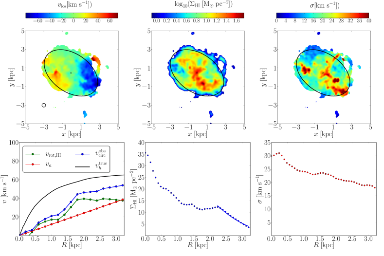
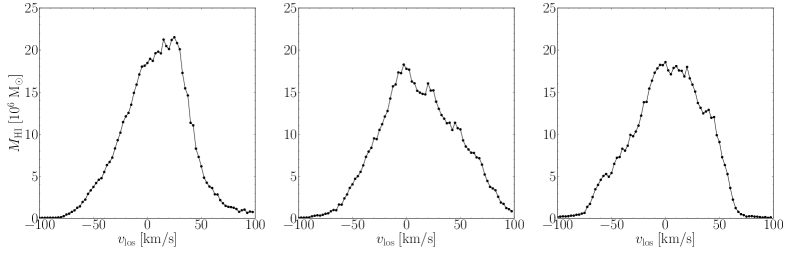
Figure 19: Same as in Fig. 3, but for M-10.

Appendix B Concentration fitting

To be able to fit the two-parameter density profiles given by Eqs. (7) and (8) to only two points (the central and outermost measured point of the rotation curve), P16 kept the concentration $c$ of the halos fixed at the mean cosmic value and used the halo mass $M_{h}$ as a free parameter. Another choice would be to fix $M_{h}$ using the stellar mass and an abundance matching relation and to keep the concentration $c$ as a free parameter.

In Fig. 20, we show the $W_{50}-v_{h,\mathrm{max}}^{\mathrm{fit}}$ relation obtained by fitting NFW and DC14 profiles to the P16 dataset, using the concentration $c$ as a free parameter with the halo mass $M_{h}$ set by the stellar mass and the Moster et al. (2013) abundance matching relation. This way, the observed galaxies adhere much more closely to the expected $W_{50}-v_{h,\mathrm{max}}^{\mathrm{true}}$ relation. NFW and DC14 profiles now actually produce very similar results.

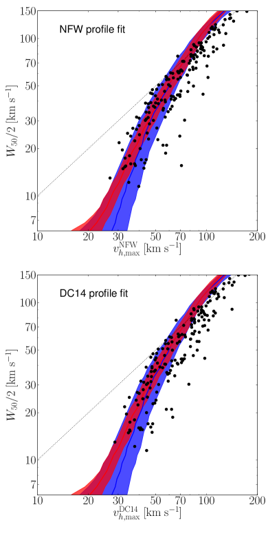
Figure 20: Results from fitting an NFW (top panel) and DC14 (bottom panel) to the outer-most point of the rotation curves of the observations used in Papastergis & Shankar (2016) using a fixed halo mass, keeping the halo concentration as a free parameter. The halo mass is calculated from their stellar mass using the abundance-matching relation of Moster et al. (2013). Red and blue lines and bands are the same as in Fig. 8.

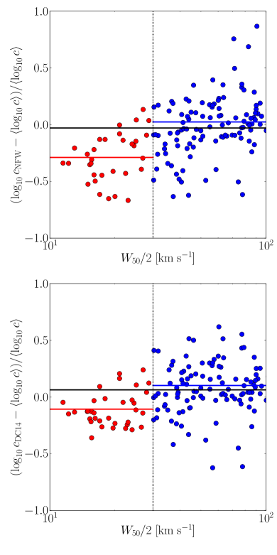
Figure 21: Logarithmic difference between the fitted concentration and the one expected from cosmological dark-matter only simulations (Dutton & Macciò 2014) of the P16 sample of galaxies. Top panel: concentration obtained by fitting the NFW density profile to the kinematic data; bottom panel: concentration obtained using the DC14 density profile. Red and blue symbols indicate galaxies with low and high H i rotation velocities, respectively. The red and blue lines indicate the mean concentration of both subsamples; the green line indicates the mean concentration of the full sample.

In Fig. 21, we compare the concentrations of the P16 galaxies retrieved in this way with the mass-dependent cosmic mean value derived from cosmological simulations (Dutton & Macciò 2014). The frequency distribution of the concentration values is well approximated with a log-normal distribution function. Both for a NFW and a DC14 fit, the scatter is $\sigma\approx 0.25-0.3$ dex. This is significantly larger than the scatter on $\log(c/\langle c\rangle)$ found in cosmological simulations, where $\sigma\sim 0.13$ (Dutton & Macciò 2014).

In Fig. 21, we distinguish between galaxies with $W_{50}/2<30\ \mathrm{km\ s^{-1}}$ (red data-points) and $W_{50}/2>30\ \mathrm{km\ s^{-1}}$ (blue data-points) for the fits with the NFW and DC14 profiles. We choose the $30\ \mathrm{km\ s^{-1}}$ split because this is the rotation velocity below which the TBTF problem becomes apparent. Clearly, the high-$W_{50}$ galaxies have higher concentrations than expected while the low-$W_{50}$ dwarfs have lower concentrations, with a hint of an anticorrelation between $M_{h}$ and concentration for the low $W_{50}$ galaxies. This is to be expected; higher-mass galaxies must have lower concentrations in order to have low circular velocities. To see whether or not the average of each subsample differs significantly from the cosmic mean value, we ran a $t$-test on both populations. We find a $p$-value of $1.1\times 10^{-8}$ for the galaxies with low $W_{50}$ in the NFW case. The full and high $W_{50}$ samples have a mean concentration consistent with the Dutton & Macciò (2014) simulations. For the DC14 profile, the same trend is found, with all the averages slightly higher than for the NFW profile. The $p$-values for the $t$-test are $3.4\times 10^{-4}$ for the entire sample and $4.3\times 10^{-7}$ and $2.2\times 10^{-4}$ for the high and low circular velocity samples, respectively. Employing the DC14 density profile yields concentration estimates that are inconsistent with the Dutton & Macciò (2014) simulations, both for the full sample and the subsamples.

Both the large scatter and the offsets are probably due, at least in part, to uncertainties on the (extrapolated) low-mass end of the $M_{\star}-M_{h}$ relation that was used to derive the halo mass from the stellar mass. In the mass regime we are interested in, the scatter on the $M_{\star}-M_{h}$ relation is expected to be substantial (e.g. Sales et al. 2017) and, using our approach, this translates in an increased scatter on the concentration parameter. Moreover, there is great variation among the different published $M_{\star}-M_{h}$ relations in the regime of dwarf galaxies ($M_{h}\approx 10^{10}\mathrm{M_{\odot}}$). Simulations also show a large scatter in stellar mass for these type of halos (e.g. Fig. 7 in V15). We redid our analysis adopting different $M_{\star}-M_{h}$ relations. Using the relation of Guo et al. (2010), we reach the same conclusions as for the relation of Moster et al. (2013); when using the relation of Behroozi et al. (2013), the fitted concentrations are more in line with the predictions from $\Lambda$CDM, however they do not follow the P16-relation.

Katz et al. (2017) fitted a NFW and a DC14-profile to 147 SPARC-galaxies, taken from a sample of 175 galaxies with extended H i rotation curves (Lelli et al. 2016). They conclude that the fitted halo masses and concentrations for the DC14-profile are in line with the predictions from $\Lambda$CDM. The difference between our analyses is that they only discuss their entire sample, which consists mostly of high-mass galaxies, whereas our analysis has focused on low-mass galaxies ($M_{\star}\lesssim 10^{8}\leavevmode\nobreak\ \mathrm{M_{\odot}}$). They also use full rotation curves to fit the halo profile to the galaxies, allowing them to fit the halo mass and concentration simultaneously.

By fitting a coreNFW profile (Read et al. 2016) to full rotation curves of a subset of the Little THINGS galaxies (Iorio et al. 2017), Read et al. (2017) find that these isolated dwarf galaxies inhabit halos consistent with the abundance-matching relation of Behroozi et al. (2013) and, as such, do not find a TBTF for isolated galaxies at all. These conclusions would change when assuming a different $M_{\star}-M_{\mathrm{halo}}$ relation, as they remark in their Appendix C. Even so, we still find that when using the relation of Behroozi et al. (2013), the observations do not follow the P16-relation.

References

- Begeman (1989) Begeman, K. G. 1989, A&A, 223, 47
- Begum et al. (2008a) Begum, A., Chengalur, J. N., Karachentsev, I. D., & Sharina, M. E. 2008a, MNRAS, 386, 138
- Begum et al. (2008b) Begum, A., Chengalur, J. N., Karachentsev, I. D., Sharina, M. E., & Kaisin, S. S. 2008b, MNRAS, 386, 1667
- Behroozi et al. (2013) Behroozi, P. S., Wechsler, R. H., & Conroy, C. 2013, ApJ, 770, 57
- Bernstein-Cooper et al. (2014) Bernstein-Cooper, E. Z., Cannon, J. M., Elson, E. C., et al. 2014, AJ, 148, 35
- Bertelli et al. (2008) Bertelli, G., Girardi, L., Marigo, P., & Nasi, E. 2008, A&A, 484, 815
- Bertelli et al. (2009) Bertelli, G., Nasi, E., Girardi, L., & Marigo, P. 2009, A&A, 508, 355
- Boylan-Kolchin et al. (2011) Boylan-Kolchin, M., Bullock, J. S., & Kaplinghat, M. 2011, MNRAS, 415, L40
- Boylan-Kolchin et al. (2012) Boylan-Kolchin, M., Bullock, J. S., & Kaplinghat, M. 2012, MNRAS, 422, 1203
- Brook & Di Cintio (2015a) Brook, C. B. & Di Cintio, A. 2015a, MNRAS, 450, 3920
- Brook & Di Cintio (2015b) Brook, C. B. & Di Cintio, A. 2015b, MNRAS, 453, 2133
- Brook & Shankar (2016) Brook, C. B. & Shankar, F. 2016, MNRAS, 455, 3841
- Brooks et al. (2017) Brooks, A. M., Papastergis, E., Christensen, C. R., et al. 2017, ArXiv e-prints
- Brooks & Zolotov (2014) Brooks, A. M. & Zolotov, A. 2014, ApJ, 786, 87
- Cai et al. (2014) Cai, R.-G., Guo, Z.-K., & Tang, B. 2014, Phys. Rev. D, 89, 123518
- Cannon et al. (2011) Cannon, J. M., Giovanelli, R., Haynes, M. P., et al. 2011, ApJ, 739, L22
- Christensen et al. (2014) Christensen, C. R., Governato, F., Quinn, T., et al. 2014, MNRAS, 440, 2843
- Cloet-Osselaer et al. (2014) Cloet-Osselaer, A., De Rijcke, S., Vandenbroucke, B., et al. 2014, MNRAS, 442, 2909
- Côté et al. (2000) Côté, S., Carignan, C., & Freeman, K. C. 2000, AJ, 120, 3027
- de Blok et al. (2008) de Blok, W. J. G., Walter, F., Brinks, E., et al. 2008, AJ, 136, 2648
- De Rijcke et al. (2013) De Rijcke, S., Schroyen, J., Vandenbroucke, B., et al. 2013, MNRAS, 433, 3005
- Di Cintio et al. (2014) Di Cintio, A., Brook, C. B., Dutton, A. A., et al. 2014, MNRAS, 441, 2986
- Di Teodoro & Fraternali (2015) Di Teodoro, E. M. & Fraternali, F. 2015, 3D-Barolo: 3D fitting tool for the kinematics of galaxies, Astrophysics Source Code Library
- Dutton & Macciò (2014) Dutton, A. A. & Macciò, A. V. 2014, MNRAS, 441, 3359
- Ferrero et al. (2012) Ferrero, I., Abadi, M. G., Navarro, J. F., Sales, L. V., & Gurovich, S. 2012, MNRAS, 425, 2817
- Garrison-Kimmel et al. (2014) Garrison-Kimmel, S., Boylan-Kolchin, M., Bullock, J. S., & Kirby, E. N. 2014, MNRAS, 444, 222
- Giovanelli et al. (2013) Giovanelli, R., Haynes, M. P., Adams, E. A. K., et al. 2013, AJ, 146, 15
- Governato et al. (2012) Governato, F., Zolotov, A., Pontzen, A., et al. 2012, MNRAS, 422, 1231
- Guo et al. (2010) Guo, Q., White, S., Li, C., & Boylan-Kolchin, M. 2010, MNRAS, 404, 1111
- Haynes et al. (2011) Haynes, M. P., Giovanelli, R., Martin, A. M., et al. 2011, AJ, 142, 170
- Heger & Woosley (2010) Heger, A. & Woosley, S. E. 2010, ApJ, 724, 341
- Hopkins et al. (2014) Hopkins, P. F., Kereš, D., Oñorbe, J., et al. 2014, MNRAS, 445, 581
- Hunter et al. (2012) Hunter, D. A., Ficut-Vicas, D., Ashley, T., et al. 2012, AJ, 144, 134
- Iorio et al. (2017) Iorio, G., Fraternali, F., Nipoti, C., et al. 2017, MNRAS, 466, 4159
- Karukes & Salucci (2017) Karukes, E. V. & Salucci, P. 2017, MNRAS, 465, 4703
- Katz et al. (2017) Katz, H., Lelli, F., McGaugh, S. S., et al. 2017, MNRAS, 466, 1648
- Kirby et al. (2012) Kirby, E. M., Koribalski, B., Jerjen, H., & López-Sánchez, Á. 2012, MNRAS, 420, 2924
- Kirby et al. (2014) Kirby, E. N., Bullock, J. S., Boylan-Kolchin, M., Kaplinghat, M., & Cohen, J. G. 2014, MNRAS, 439, 1015
- Klypin et al. (2015) Klypin, A., Karachentsev, I., Makarov, D., & Nasonova, O. 2015, MNRAS, 454, 1798
- Lelli et al. (2016) Lelli, F., McGaugh, S. S., & Schombert, J. M. 2016, AJ, 152, 157
- Lelli et al. (2017) Lelli, F., McGaugh, S. S., Schombert, J. M., & Pawlowski, M. S. 2017, ApJ, 836, 152
- Lelli et al. (2012) Lelli, F., Verheijen, M., Fraternali, F., & Sancisi, R. 2012, A&A, 544, A145
- Macciò et al. (2016) Macciò, A. V., Udrescu, S. M., Dutton, A. A., et al. 2016, MNRAS, 463, L69
- Mamon et al. (2017) Mamon, A. A., Bamba, K., & Das, S. 2017, European Physical Journal C, 77, 29
- McGaugh et al. (2016) McGaugh, S. S., Lelli, F., & Schombert, J. M. 2016, Physical Review Letters, 117, 201101
- Moster et al. (2013) Moster, B. P., Naab, T., & White, S. D. M. 2013, MNRAS, 428, 3121
- Navarro et al. (1996) Navarro, J. F., Frenk, C. S., & White, S. D. M. 1996, ApJ, 462, 563
- Oh et al. (2011) Oh, S.-H., de Blok, W. J. G., Brinks, E., Walter, F., & Kennicutt, Jr., R. C. 2011, AJ, 141, 193
- Oh et al. (2015) Oh, S.-H., Hunter, D. A., Brinks, E., et al. 2015, AJ, 149, 180
- Papastergis et al. (2015) Papastergis, E., Giovanelli, R., Haynes, M. P., & Shankar, F. 2015, A&A, 574, A113
- Papastergis & Ponomareva (2016) Papastergis, E. & Ponomareva, A. A. 2016, ArXiv e-prints