Valence quark contributions for the $\gamma^{\ast}N\to N(1440)$ form factors
from Light-Front holography

Abstract

The structure of the nucleon and the first radial excitation of the nucleon, the Roper, $N(1440)$, is studied within the formalism of Light-Front holography. The nucleon elastic form factors and $\gamma^{\ast}N\to N(1440)$ transition form factors are calculated under the assumption of the dominance of the valence quark degrees of freedom. Contrary to the previous studies, the bare parameters of the model associated with the valence quark are fixed by the empirical data for large momentum transfer ($Q^{2}$) assuming that the corrections to the three-quark picture (meson cloud contributions) are suppressed. The $\gamma^{\ast}N\to N(1440)$ transition form factors are then calculated without any adjustable parameters. Our estimates are compared with results from models based on valence quarks and others. The model compares well with the $\gamma^{\ast}N\to N(1440)$ transition form factor data, suggesting that meson cloud effects are not large, except in the region $Q^{2}<1.5$ GeV². In particular, the meson cloud contributions for the Pauli form factor are small.

I Introduction

Within the nucleon excited states ($N^{\ast}$) the $N(1440)$ resonance, also known as Roper, plays a special role. Contrarily to the $\Delta(1232)$ and other nucleon excitations, the Roper was not identified as a bump in a reaction cross-section but was instead found in the analysis of phase-shifts Roper64 . Nowadays there is evidence that the Roper should be identified as the first radial excitation of the nucleon quark core, although meson excitations are also important for the internal structure.

Calculations based on valence quark degrees of freedom are consistent with the $\gamma^{\ast}N\to N(1440)$ transition form factors for large $Q^{2}$ ($Q^{2}>2$ GeV²) Aznauryan07 ; Roper ; Roper2 ; Roper-APS ; Segovia15 ; Santopinto12 . However, estimates based exclusively on quark degrees of freedom fail to describe the small $Q^{2}$ data ($Q^{2}<2$ GeV²) Aznauryan07 ; NSTAR ; Aznauryan12 . The gap between valence quark models and the data at low $Q^{2}$ has been interpreted as the manifestation of the meson cloud effects Roper ; Roper2 ; Segovia15 ; Aznauryan12b . When the meson cloud contributions are included in quark models the estimates approach the data Cano98 ; Tiator04 ; Li06 ; Chen08 ; Golli09 ; Obukhovsky11 .

Besides, the calculations based on dynamical coupled-channel reaction models, where the baryon excitations are described as baryon-meson states with extended baryon cores Burkert04 ; EBAC , corroborates the importance of the meson cloud effects. In those models the mass associated with the Roper bare core is about 1.7 GeV. Only when the meson cloud dressing is considered the Roper mass is reduced to the experimental value Suzuki10 . The interpretation of the Roper as a radial excitation of the nucleon combined with a dynamical meson cloud dressing solves the long standing problem of the Roper mass in the context of a quark model Capstick00 .

The Roper decay widths into $\gamma N$, $\pi N$ and $\pi\pi N$ are large comparative to other $N^{\ast}$ decays. Those decay widths are also difficult to explain in the context of a quark model. The meson cloud dressing helps to explain the $N(1440)\to\gamma N$ width, where the contributions associated with baryon-meson-meson states play an important role Suzuki10 ; Gegelia16 ; Golli09 ; Chen08 .

Overall the recent developments in the study of the Roper electromagnetic structure point to the picture of a radial excitation of the nucleon surrounded by a cloud of mesons Suzuki10 ; Golli09 ; Bauer14 ; Wang17 ; Roberts14a ; Aznauryan12b . There is therefore a strong motivation to study the Roper internal structure and to disentangle the effects of the valence quark component from the meson cloud component. In particular, one can use the knowledge of the baryon core structure to infer the contribution due to the meson cloud. This procedure was used in previous works based on different frameworks for the baryon core Roper ; Roper2 ; Segovia15 ; Aznauryan12b .

In the case of the nucleon the valence quark degrees of freedom produce the dominant effect in the elastic form factors. The meson cloud contribution to the nucleon wave function is estimated to be of the order of a few percent Perdrisat07 ; Nucleon ; Octet ; Medium . As for the Roper, the meson cloud seems to play a more prominent role. We conclude at the end that the valence quark degrees of freedom provide a very good description of the data, but the meson cloud contribution are important below 1.5 GeV², particularly for the Dirac form factor.

In the present work we propose a new framework to analyze the role of the valence quarks and the meson cloud in the Roper. We use Light-Front holography to estimate the leading order (lowest Fock state) contribution to the $\gamma^{\ast}N\to N(1440)$ transition form factors. Since the leading order calculation includes only pure valence quark effects in the baryon wave functions ($qqq$ contributions), there is no contribution from the meson cloud. In those conditions the gap between the calculations and the data must be essentially the consequence of the meson cloud effects.

The Light-Front (LF) formalism is particularly appropriate to study hadron systems, ruled by QCD, and to describe the hadronic structure in terms of the constituents Teramond09a ; Brodsky15 ; Teramond12a ; Teramond11a . The LF wave functions (LFWF) are relativistic and frame independent Brodsky98 ; Brodsky15 . The connection between LF quantization of QCD and anti-de Sitter conformal field theory (AdS/CFT) leads to Light-Front holography Teramond12a ; Brodsky15 ; Brodsky08a . LF holography have been used to study the structure of hadron properties, such as the hadron mass spectrum, parton distribution functions, meson and baryon form factors etc. NSTAR ; Teramond12a ; Chakrabarti14a ; Brodsky15 ; Teramond13a ; Teramond15a ; Forkel07 ; Karch06 ; Ballon12 ; Grigoryan09 ; Grigoryan07a ; Bayona15a ; Brodsky06 ; Brodsky08a ; Branz10a ; Vega11 ; Ahmady16 ; Mamedov16 ; NucleonAxial ; Vega11a . In particular, the formalism was recently applied to the study of the nucleon Hong08a ; Abidin09 ; Gutsche12a ; Chakrabarti13a ; Liu15a ; Maji16a ; Sufian17a and Roper Teramond11a ; Teramond12a ; Gutsche13a electromagnetic structure.

An important advantage of the LF formalism applied to hadronic physics is the systematic expansion of the wave functions into Fock states with different number of constituents Brodsky01 ; Brodsky98 ; Brodsky15 . In the case of the baryons the leading order contributions is restricted to the three-valence quark configuration. Although the restriction to the lowest order Fock state (three valence-quark system) may look as a rough simulation of the real world, it may provide an excellent first approximation when the confinement is included in the LFWF, defined at the Light-Front time Brodsky08a ; Perdrisat07 ; Teramond15a . In those conditions non-perturbative physics is effectively taken into account by LF holography Brodsky15 ; Teramond15a .

Under the assumption that LF holography can describe accurately the large-$Q^{2}$ region dominated by valence quark degrees of freedom, we calibrate the free parameters of the model by the available data above a given threshold $Q^{2}\geq Q_{m}^{2}$ ($Q_{m}^{2}=1.5$–2.5 GeV²). This procedure differs from the previous studies where the free parameters, associated with the nucleon anomalous magnetic moments were fixed at $Q^{2}=0$, where the meson cloud contamination is expected to be stronger. Once the free parameters are fixed by the nucleon data, one uses the model to calculate the $\gamma^{\ast}N\to N(1440)$ transition form factors. Since no parameter is adjusted by the Roper data, our calculations are true predictions for the $\gamma^{\ast}N\to N(1440)$ transition form factors.

This article is organized as follows: In Sec. II we review the LF setup originally used in Ref. Abidin09 in the context of calculation of baryon form factors. In Secs. III and IV we adapt the calculations of Refs. Gutsche12a ; Gutsche13a to derive our main results. In particular, in Sec. III, we review the results for the nucleon form factors and fix the parameters by the nucleon data. Sec. IV contains our results for the valence quark contribution to the $\gamma^{\ast}N\to N(1440)$ transition form factors and their discussion. The outlook and conclusions are presented in Sec. V.

II Light-Front holography

It is by now well known that string theory or gravity in anti-de Sitter (AdS) space can provide a description of some lower-dimensional (conformal) gauge theories (CFT) at strong coupling Maldacena97 ; Gubser98 ; Witten98 . This AdS/CFT correspondence, or holography, can, with certain important restrictions, be applied to QCD-like theories, e.g. Witten98b ; Klebanov00 ; Sakai04 . It remains an open question, however, whether the top-down string theory methods are practical enough to model QCD itself. Instead it proved efficient to apply bottom-up approaches to QCD Erlich05 ; DaRold05 ; Karch06 . Such approaches are motivated phenomenologically by the string models, but lack a first-principle justification. Among those, the approach of LF holography is based on a comparison of the results of the LF quantization of QCD DrellYan ; West with the predictions of holographic (AdS/CFT) models Teramond12a ; Brodsky15 ; Gutsche12a ; Chakrabarti13a ; Liu15a ; Hong07a .

II.1 Light-Front QCD vs AdS/CFT

Light-Front quantization provides a powerful tool to study systems ruled by microscopic QCD dynamics. It starts with introducing a special (Light-Front) parametrization of the Hamiltonian, which consequently acts on a Hilbert space of the LF wave functions spanned by partonic Fock states associated with quarks and gluons Teramond12a ; Brodsky15 .

The Fock states $|n\rangle$ are multi-particle eigenstates of the free Hamiltonian for the constituent quarks and gluons. Their coefficients $\psi_{n}(\varkappa_{i},{\bf k}_{\perp i})$ in the LFWF expansion depend on the fraction of momentum $\varkappa_{i}$ of partons, $i=1,\ldots,n$, as well as the partons transverse momenta ${\bf k}_{\perp i}$ Brodsky15 ; Brodsky06 . The notation $\psi_{n}(\varkappa_{i},{\bf k}_{\perp i})$ implies a dependence on the fractions $\varkappa_{i}$ and transverse momenta of all the partons.

In the standard terminology $|n\rangle$ are the states of a given twist $\tau\equiv n$. The amplitudes $\psi_{n}(\varkappa_{i},{\bf k}_{\perp i})$ define the probability to find the hadron in the given $n$-parton Fock state. The Fock state expansion separates the dependence on bound state total four-momentum $P$, contained in $|n\rangle$, from the frame-invariant dependence on the relative variables $\varkappa_{i}$ and ${\bf k}_{\perp i}$, which are subject to the conditions $\sum_{i=1}^{n}\varkappa_{i}=1$ and $\sum_{i=1}^{n}{\bf k}_{\perp i}={\bf 0}$ Liu15a ; Brodsky15 . A useful representation of amplitudes is in terms of the conjugate impact space, obtained by a 2D Fourier transform to $\widetilde{\psi}_{n}(\varkappa_{i},{\bf b}_{\perp i})$, which depends on the impact parameters ${\bf b}_{\perp i}$, satisfying $\sum_{i=1}^{n}{\bf b}_{\perp i}={\bf 0}$ Brodsky06 ; Brodsky15 .

The relativistic LF eigenvalue equation $H_{LF}|\Psi_{h}\rangle=M_{h}^{2}|\Psi_{h}\rangle$, for the LFWF $|\Psi_{h}\rangle$ of the hadron $h$, can be cast in a form of a Schrödinger-like equation for $\widetilde{\psi}_{n}(\varkappa_{i},{\bf b}_{\perp i})$, where the Hamiltonian $H_{LF}$ can be separated into particle kinematic terms and a complicated (unknown) interaction potential for the constituents. For practical purposes it is natural to reduce this hadron system down to a system where the parton is subject to an simplified one-body potential which captures the effect of confinement Liu15a ; Brodsky15 ; Teramond09a .

In the study of electromagnetic interaction in impulse approximation one can regard a baryon as a system of an active quark and a cluster of $(n-1)$ spectator partons. In this conditions the amplitudes of the Fock states can be reduced to $\widetilde{\psi}_{n}(\varkappa,{\bf b}_{\perp})$, where $\varkappa$ (respectively $1-\varkappa$) and ${\bf b}_{\perp}$ ($-{\bf b}_{\perp}$) are the variables associated with the active quark (spectator cluster), so that $\widetilde{\psi}_{n}(\varkappa,{\bf b}_{\perp})$ can be interpreted as the wave function of a two-body quark-cluster system Liu15a ; Sufian17a ; Teramond09a ; Brodsky15 .

In the case of the baryons, in leading twist approximations ($\tau=n=3$) and massless quarks, one can reduce the LF wave equation to the form Liu15a ; Teramond09a ; Brodsky15 ; Sufian17a

$$\left[-\frac{\nabla^{2}_{{\bf b}_{\perp}}}{\varkappa(1-\varkappa)}+U_{\rm eff}\right]\tilde{\psi}_{n}(\varkappa,{\bf b}_{\perp})=M_{h}^{2}\tilde{\psi}_{n}(\varkappa,{\bf b}_{\perp}),$$ (1)

where the effective potential $U_{\rm eff}=\mu_{J}+\Phi$ consists of the effective potential $\mu_{J}$, encoding the total angular momentum $J$ of the hadron, and the effective interaction potential $\Phi$, exhibiting confinement Brodsky15 . The kinetic term in the equation also encodes the relative angular momentum $L$ of the quark-spectator system ($L=0,1$) Liu15a ; Brodsky06 ; Brodsky15 .

Furthermore, in the semiclassical approximation, when the quarks have no mass and the quark loops are neglected, one can replace the dependence on the variables $\varkappa$ and ${\bf b}_{\perp}$ in $\widetilde{\psi}_{n}$ by the dependence on a single parameter $\zeta=\varkappa(1-\varkappa)|{\bf b}_{\perp}|$, except for an overall factor $f(\varkappa)=\sqrt{\varkappa(1-\varkappa)}$ Brodsky06 ; Brodsky15 ; Liu15a . The LF wave equation associated with $\widetilde{\psi}_{n}(\varkappa,\zeta)$ then becomes a one-dimensional Schrödinger equation in the “radial” variable $\zeta$. The variable $\zeta$ measures the separation between the active quark and the remaining spectator partons. In the case of $n$-body systems $\zeta$ appears to be a $\varkappa$-weighted average of the impact variables: $|{\bf b}_{\perp}|\to|\sum_{j=1}^{n-1}\varkappa_{j}{\bf b}_{\perp j}|/|\sum_{j=1}^{n-1}\varkappa_{j}|$ Brodsky06 ; Brodsky15 ; Sufian17a .

The key observation of LF holography is the equivalence of the Schrödinger equation for the LFWFs $\widetilde{\psi}_{n}(\varkappa,\zeta)$ and the characteristic equations of matter fields in five-dimensional anti-de Sitter (AdS₅) space, assuming that one identifies $\zeta$ with the radial coordinate of AdS₅, $z$ Brodsky06 ; Radyushkin95 ; Brodsky15 . For that correspondence contributes the fact that the residual $\varkappa$ dependence in the wave function factorize, and can be absorbed in the normalization factors in the 5D theory calculation of matrix elements. Consequently, the $\varkappa$ dependence is not relevant for the holographic correspondence.

The purpose of this work is to understand the leading twist contribution ($\tau=3$) for the nucleon and Roper, which corresponds to the valence quark approximation to certain QCD processes. To study the electromagnetic properties of the nucleon radial excitations we use the two-body decomposition of the three-quark systems ($\tau=3$), representing those systems as an active quark and a spectator cluster with masses (eigenvalues) and wave functions determined by the holographic equivalents of LF wave equation, as described above. The AdS wave equation used in the present work is discussed in the next sections.

II.2 5D fermion in AdS space

In the bottom-up holographic approach to QCD the nucleon and the nucleon excitations can be introduced as fermion fields in five-dimensional AdS space Hong07a ; Hong07 . To define this curved space one requires the metric tensor $g$, which can be conveniently introduced via line element $ds^{2}$ in the Poincaré coordinates:

$$ds^{2}\ =\ \frac{R^{2}}{z^{2}}\left(\eta_{\mu\nu}dx^{\mu}dx^{\nu}-dz^{2}\right),$$ (2)

where $\eta_{\mu\nu}=\text{diag}(+,-,-,-)$ is the 4D Minkowski metric tensor and $R$ is a parameter called AdS radius. The latter sets the scale for the space’s curvature. AdS₅ radial coordinate $z$ is to be identified with the LF parameter $\zeta$.

From the metric one can define the Dirac operator $\hat{\cal D}$, which we write as

$$\hat{\cal D}=\frac{i}{2}\,e^{M}_{A}\Gamma^{A}\left({\overleftrightarrow{\partial}_{M}}+{\textstyle\frac{1}{8}}\omega_{M}^{AB}[\Gamma^{A},\Gamma^{B}]\right).$$ (3)

Here $\Gamma^{A}$, $A,B=0,1,2,3,z$ is the standard set of five Dirac gamma matrices and we choose to represent in the chiral basis. Frame $e^{M}_{A}$ and spin-connection $\omega_{M}^{AB}$ tensor fields can be computed from the metric tensor. For completeness we summarize the explicit formulas here

$$e_{A}^{M}\Gamma^{A} = \frac{z}{R}(\gamma^{\mu},-i\gamma_{5})\,,$$ (4)

$$\omega_{M}^{AB} = \frac{1}{z}(\eta^{Az}\delta_{M}^{B}-\eta^{Bz}\delta_{M}^{A})\,$$ (5)

It is also understood that $A{\overleftrightarrow{\partial}}_{M}B=A(\partial_{M}B)-(\partial_{M}A)B.$

Substantiating the above claim, the kinematic properties of nucleons, e.g. the spectrum, can be described by a theory of a massive fermion in AdS₅:

$$S_{N} = \int d^{4}x\,dz\ \sqrt{-\mbox{det}\;g}\;\overline{\Psi}\big{(}\hat{{\cal D}}-\mu-\Phi\big{)}\Psi\,,$$ (6)

where $\mu$ is the 5D fermion mass to be fixed below.

The function $\Phi(z)$ is an effective scalar potential, whose role is to introduce the complex dynamics of QCD, essentially the confinement. When $\Phi=0$, the equations of motion of the 5D theory can be cast in the form corresponding to the LF Schrödinger equation in the conformal limit Brodsky15 . A phenomenologically compelling choice of the potential is Abidin09 ; Gutsche12a

$$\Phi=\kappa^{2}z^{2}\,.$$ (7)

The dimensionful parameter $\kappa$ breaks conformal symmetry and introduces a mass scale, which determines the meson and baryon spectrum Teramond12a ; Brodsky15 ; Teramond15a . It can be thus related to $\Lambda_{\rm QCD}$. A conventional way to introduce this potential is through the dilaton field background Abidin09 ; Gutsche12b . This procedure makes the connection with top-down AdS/CFT constructions. The corresponding bottom-up case is dubbed the soft-wall model.

In four dimensions the four-component Dirac spinor describes two independent chirality modes. Although five-dimensional Dirac spinor $\Psi$ equally has four components, it will correspond to a nucleon with a specific single choice of chirality. This is a consequence of boundary conditions necessary in the holographic approach Henningson98 ; Mueck98 ; Henneaux98 ; Abidin09 ; Gutsche12a ; Hong07a . In order to preserve CP invariance, the second chirality mode is introduced similarly as Eq. (6), but with an opposite sign in front of $\mu$ and $\Phi$, e.g. Gutsche12a . For simplicity of presentation we only review one chirality mode here.

II.3 Wave equations and wave functions

In order to solve the Dirac equations derived from action (6) the fermion field (spin 1/2 and positive parity) $\Psi$ is decomposed into its left- and right- chirality components:

$$\Psi(x,z)=\Psi_{L}(x,z)+\Psi_{R}(x,z),$$ (8)

where $\Psi_{L/R}={\textstyle\frac{1}{2}}(1\mp\gamma^{5})\Psi$. The solution can then be found via separation of variables, assuming a plane wave dependence on the 4D spacetime coordinates

$$\Psi_{L/R}(x,z)\ =\ \psi_{L/R}(x)z^{2}F_{L/R}(z)\,,$$ (9)

where left and right Weyl spinors $\psi_{L/R}(x)=\psi_{L/R,P}\,e^{iP\cdot x}$ satisfy the 4D Dirac equation with mass $M^{2}=P^{2}$. We also pull out the $z^{2}$ factor for convenience. In the end, one is left with a pair of coupled equations for scalar profile functions $F_{L/R}(z)$:

$$\left[\pm\partial_{z}+\frac{\mu R+\Phi}{z}\right]F_{L/R}(z)=M\,F_{R/L}(z)\,.$$ (10)

The equations must be solved with an appropriate choice of boundary conditions. First, holography requires regularity of the wave function $\Psi(x,z)$ as $z\to\infty$. For $z\to 0$ there are two linearly independent solutions $F_{L/R}\sim z^{\mp\mu R}$. In holography one usually chooses to call one of those solutions the source and another one the vev of the operator dual to the bulk (5D) field $\Psi$ – in this case baryon interpolating operator. For the problem in question it only makes sense to choose the vev solution as $F_{R}\sim z^{\mu R}$ and the source $F_{L}=0$. The opposite choice, source $F_{R}=0$ and vev $F_{L}\sim z^{-\mu R}$ leads to a non-physical spectrum. Note that for the opposite chirality case one changes $\mu\to-\mu$, and the two choices of the $z\to 0$ boundary conditions are interchanged, with the physical one being $F_{R}=0$ and $F_{L}\sim z^{\mu R}$.

After fixing the boundary conditions it is standard to rewrite system (10) as a second order Schrödinger-like differential equation for either $F_{R}$, or $F_{L}$. Since we are solving the boundary problem, any solution can be expanded over an eigenfunction basis, labeled by an integer $n$. Equation

$$-\frac{d^{2}}{dz^{2}}F_{R}+\frac{m(m-1)}{z^{2}}\,F_{R}+2\kappa^{2}\left(m+\frac{1}{2}\right)F_{R}\\ +\kappa^{4}z^{2}F_{R}=M_{n}^{2}F_{R},$$ (11)

has a set of eigenfunctions $F_{L/R,n}(z)$ expressed in terms of the generalized Laguerre polynomials $L_{n}^{\alpha}$:

$$F_{R,n}(z)\ \propto\ z^{m}e^{-\kappa^{2}z^{2}/2}L_{n}^{m-1/2}(\kappa^{2}z^{2}).$$ (12)

The second component $F_{L}$ can now be calculated using Eqs. (10):

$$F_{L,n}(z)\ \propto\ z^{m+1}e^{-\kappa^{2}z^{2}/2}L_{n}^{m+1/2}(\kappa^{2}z^{2}).$$ (13)

These eigenfunctions correspond to eigenvalues given by

$$M_{n}^{2}=4\kappa^{2}\left(n+m+\frac{1}{2}\right).$$ (14)

We recall that in the previous expressions $m\equiv\mu R$.

The eigenvalues provide the result for the 4D spectrum of nucleon excitations with radial excitation quantum number $n$ and angular momentum quantum number linear in the parameter $m$, which we will fix below. The above choice of the potential (7) leads to the spectrum consistent with Regge trajectories Teramond12a ; Brodsky15 ; Karch06 .

Summing up, the full solution for the 4D positive chirality mode reads

$$\Psi_{n}^{+}(x,z)=z^{2}\left(\begin{array}[]{c}F_{L,n}(z)\,\chi_{n}(x)\\ F_{R,n}(z)\,\chi_{n}(x)\\ \end{array}\right),$$ (15)

where $\chi_{n}(x)$ are two component spinors related with the Weyl spinors: $\psi_{L}^{\dagger}(x)=(\chi_{n}^{\dagger}(x),0)$ and $\psi_{R}^{\dagger}(x)=(0,\chi_{n}^{\dagger}(x))$. The negative chirality modes is obtained via an appropriate change of signs and exchange of the solutions for $F_{L/R}$ Gutsche12a ; Gutsche13a :

$$\Psi_{n}^{-}(x,z)=z^{2}\left(\begin{array}[]{c}F_{R,n}(z)\,\chi_{n}(x)\\ -F_{L,n}(z)\,\chi_{n}(x)\\ \end{array}\right).$$ (16)

Using the component associated with the index $n$ we can write the fermion fields with positive and negative parities as

$$\Psi^{\pm}(x,z)=\frac{1}{\sqrt{2}}\sum_{n}\Psi_{n}^{\pm}(x,z).$$ (17)

II.4 Interactions

In hadron physics, information on the structure of nucleon resonances is contained in the matrix elements of interaction currents between the initial and final hadrons, including the nucleon and the nucleon excitations (baryons). In holography, 4D operators of conserved currents $J_{\mu}$ are described by massless gauge fields $V_{M}$ in AdS₅ space. Interacting bulk baryon fields $\Psi$ couple to the gauge fields, which is a dual holographic description of the coupling of baryons to conserved currents. Matrix elements of the currents, can be computed from the interaction terms, which are, schematically, overlaps of the bulk fields with the source gauge field Strassler01 :

$$S_{\rm int}=\int d^{4}x\,dz\,\sqrt{-\det g}\;\bar{\Psi}(x,z)\,\hat{\cal V}(x,z)\Psi(x,z).\quad$$ (18)

Here $\hat{\cal V}$ encodes a coupling of field $V_{M}$ to fermions. We consider in particular the decomposition

$$\hat{\cal V}(x,z)=\hat{\cal V}_{0}(x,z)+\hat{\cal V}_{1}(x,z)+\hat{\cal V}_{2}(x,z),$$ (19)

as discussed next. For simplicity, we only present the interaction for positive chirality. For the opposite chirality case one has to adjust the signs in the above expression to preserve the CP invariance Gutsche12a .

The term $\hat{\cal V}_{0}(x,z)$ is representing the minimal Dirac coupling given by Abidin09

$$\hat{\cal V}_{0}(x,z)=\hat{Q}\,\Gamma^{M}V_{M}(x,z),$$ (20)

where $V_{M}$ could be either the abelian dual of the electromagnetic current, or the non-abelian isovector current. Following the parametrization of Gutsche12a ; Gutsche13a $\hat{Q}=e_{N}={\textstyle\frac{1}{2}}(1+\tau_{3})$, the nucleon charge ($N=p,n$), for the elastic electromagnetic transitions, and $\hat{Q}=\tau_{3}$ for the transition between the nucleon and higher mass $J^{P}=\frac{1}{2}^{+}$ resonances ($\tau_{3}$ is the Pauli isospin operator). This minimal coupling only yields the Dirac form factor.

To produce the Pauli form factor more input from the holographic side is necessary. Abidin and Carlson Abidin09 proposed to consider a non-minimal extension of the coupling $\hat{\cal V}_{0}$, adding a term

$$\hat{\cal V}_{1}(x,z)\ =\ \frac{i}{4}\,\eta_{N}[\Gamma^{M},\Gamma^{N}]V_{MN}(x,z)\,,$$ (21)

where $V_{MN}=\partial_{M}V_{N}-\partial_{N}V_{M}+[V_{M},V_{N}]$ and one can consider different couplings $\eta_{S}$ and $\eta_{V}$ for the isoscalar and isovector parts respectively [$\eta_{N}={\textstyle\frac{1}{2}}(\eta_{S}+\eta_{V}\tau_{3})$]. As one may expect from its Lorentz structure, this term yields the Pauli form factors, as well as a correction to the Dirac form factors. Moreover, since the non-minimal term contains derivatives of the field $V_{M}$ and extra powers of $z$, the Pauli form factor turns out to be subleading with respect to the Dirac form factor at large momentum transfer, as expected, while the correction to the Dirac form factor is of the same order. The effect of the term ${\cal V}_{1}$ on the nucleon form factors is studied in Refs. Teramond12a ; Chakrabarti13a ; Abidin09 ; Gutsche12a ; Gutsche13a ; Maji16a . We provide additional details in what follows.

More couplings can be considered. In Refs. Gutsche12a ; Gutsche13a the following minimal-type (isovector) coupling was suggested

$$\hat{\cal V}_{2}(x,z)\ =g_{V}\tau_{3}\,\Gamma^{M}\gamma^{5}V_{M}(x,z)\,.$$ (22)

where $g_{V}$ is a coupling constant. This coupling is consistent with gauge invariance and discrete symmetries, that can be added to the 5D action to improve the fitting of experimental data Gutsche12a .

One first observation about this term is that it naively breaks CP in 4D. However, this is not the case, since 5D fermion $\Psi$ describes only one 4D chirality. Adding a similar interaction term for the opposite chirality, with the opposite sign of coupling, ensures 4D CP invariance.

A more serious issue is that Eq. (22) breaks 5D covariance. Adding such term requires an implicit background 5D vector field. Such background fields are more common in the higher-dimensional top-down holographic models with flux compactifications. Here we assume that such a flux compactification exists and we assess its effect on the observable form factors. We further comment on the general structure of the term (18) in Ref. inpreparation .

In order to calculate transition matrix elements of the currents using Eq. (18) one needs to specify the 5D gauge field $V_{M}(x,z)$. Similarly to fermions, a bosonic gauge field dual to the isovector or isoscalar current is introduced by a 5D Lagrangian. Specifically, one needs to solve equations following from the action

$$S_{J}\ =\ -\int d^{4}x\,dz\,\sqrt{-\det g}\,\frac{e^{-\Phi}}{4}\,{\rm Tr\,}V_{MN}V^{MN}\,,$$ (23)

subject to appropriate boundary conditions. These boundary conditions differ from the boundary conditions for the fields associated with the nucleon and the nucleon excitations, since they have to be of the source type at $z=0$ (the leading solution as opposed to the subleading vev-type). The regularity condition requires $V_{M}$ to vanish for $z\to\infty$.

In what follows we will be interested in the abelian electromagnetic current, so the non-abelian details of this discussion can be omitted. Altogether, the solution can be cast in the form Grigoryan07b ; Gutsche12a ; Gutsche13a

$$V_{\mu}(x,z)\ =\ \int\frac{d^{4}q}{(2\pi)^{4}}\,e^{-iq\cdot x}\epsilon_{\mu}(q)V(-q^{2},z)\,,$$ (24)

where $\epsilon_{\mu}$ is the photon polarization vector, and

$$V(Q^{2},z)=\kappa^{2}z^{2}\int_{0}^{1}\frac{d\varkappa}{(1-\varkappa)^{2}}x^{\frac{Q^{2}}{4\kappa^{2}}}e^{-\frac{\kappa^{2}z^{2}\varkappa}{1-\varkappa}}\,,$$ (25)

with $Q^{2}=-q^{2}$. In the limit $z\to 0$, one has $V(Q^{2},0)=1$.

Substituting Eqs. (24) and (25) together with the modes (15) and (16) into the interaction Lagrangian (18) yields matrix elements of the current up to some normalization terms, from which form factors are read off directly. We spare the reader the details of this analytical calculation, but rather summarize the final results in Sec. III for the nucleon and in Sec. IV for the Roper. See Refs. Gutsche12a ; Gutsche13a for the original derivation.

II.5 Mass spectrum and more

In this section we specify the details of the holographic model and relating it to the observable spectrum of the nucleon radial excitations and the $\rho$ mesons.

First, the nucleon ($\Psi_{N0}$) and the Roper ($\Psi_{N1}$) are the states with radial quantum numbers $n=0,1$ and angular momentum $L=0$. Any of these states must be regarded as a superposition of the given twist (number of partons) Fock states, so we assume that the 5D mass $\mu$ is encoding both the angular momentum $L$ and the twist $\tau$, $\mu R=m(L,\tau)$.

A way to fix the relation for $L=0$ is to analyze the large $Q^{2}$ scaling of $F_{L/R,n}(z)$ and consequently the form factors. As discussed later, the choice $m=\tau-3/2$ yields the correct falloff estimated by perturbative QCD (pQCD) Carlson . Consequently, the spectrum (14) takes the following form Teramond12a ; Gutsche13a ; Brodsky15 ,

$$M_{Nn}=2\kappa\sqrt{n+\tau-1}\,.$$ (26)

Thus, holography provides an estimate for the spectrum of the nucleon radial excitations in terms of a single scale parameter $\kappa$. Similarly, one obtains the spectrum of mesons and baryons with different angular momenta and parity Teramond12a ; Brodsky15 ; Teramond15a .

The $\rho$ meson (mass $m_{\rho}$) is a traditional reference for the hadron states. In LF holography we can write $m_{\rho}=2\kappa$. The nucleon mass, for example, approximately satisfies $M_{N}=\sqrt{2}m_{\rho}$. If we assume that the nucleon mass is primarily composed of the leading twist $\tau=3$ contribution, $M_{N}=2\sqrt{2}\kappa$, then the phenomenological value of $\kappa$ is fixed at

$$\kappa\ =\ \frac{m_{\rho}}{2}\sim\Lambda_{\rm QCD}\,.$$ (27)

The leading twist estimate of the masses of nucleon radial radial excitations is now given by $M_{Nn}=2\kappa\sqrt{n+2}$, $n=0,1,2...$. This yields $M_{R}=M_{N1}=2\sqrt{3}\kappa$ for the Roper mass in leading twist approximation ($\tau=3$).

It is worth mentioning that the LF estimate of the Roper mass, $M_{R}\simeq\sqrt{3}m_{\rho}$, is not so accurate as for the nucleon and the $\rho$ meson. This is consistent with a general expectation that leading twist approximation is not so accurate for baryons as it is for mesons. In particular for the Roper, there are indications that the baryon-meson-meson corrections of the twist order $\tau=7$ are important Suzuki10 ; Gegelia16 . In the next subsection we collect further comments on the spectrum and other issues of LF holography.

The spectrum of the hadrons, as predicted by LF holographic approach has further issues. A similar approach to mesons yields similar Regge-behaved spectra as the one given by Eq. (26). For the $\rho$ meson family one gets $m_{\rho n}=2\kappa\sqrt{n+1}$ for $n=0,1,2,\ldots$ Grigoryan07b ; Branz10a ; Karch06 . Brodsky and Teramond argue, however, that those twist-2 mass poles should be shifted to their physical values, suggesting that $m_{\rho n}=2\kappa\sqrt{2n+1}$ Teramond15a ; Brodsky15 ; Sufian17a . These formula gives a very good agreement with the vector meson masses for $\kappa\simeq 0.385$ GeV Teramond15a ; Brodsky15 , as in Eq. (27), provided that $m_{\rho}\simeq 770$ MeV. Similar values were used in Refs. Gutsche12a ; Gutsche13a .

II.6 Comments on interpolating operators in LF holographic approach

The scaling dimension $\Delta$ is defined by the behavior of the wave function in the limit $z\to 0$: $\Psi(x,z)\sim z^{\Delta}$ Abidin09 ; Brodsky08a . The holographic approach relates the 5D mass parameter $m$ with the scaling dimension $\Delta$ of the hadron interpolating operator. For example, for the vector field this relation is

$$\Delta\ =\ 2+\sqrt{m^{2}+1}\,.$$ (28)

For the massless vector field $V_{M}$ above, this infers $\Delta=3$, the correct scaling dimension of a current operator Brodsky08a . For fermions however the relation is

$$\Delta=2+|m|\,.$$ (29)

In the leading twist this yields $\Delta=7/2$ for the nucleon/Roper interpolating operator, in contrast to the scaling dimension $\Delta_{\cal O}=9/2$ of the operator ${\cal O}=qqq$, composed of three quark fields. This discrepancy is even more pronounced if one applies the identification $m(\tau,L)$ used in Ref. Brodsky15 . Indeed, comparing Eqs. (12) and (14) with Eqs. (5.34) and (5.38) of Ref. Brodsky15 one ends up with the relation $m=\nu+1/2$, which implies $\Delta=5/2$.

In QCD the (anomalous) scaling dimensions of the interpolating operators are not well-defined, because of the logarithmic running of the gauge coupling. In a putative conformal theory, which would approximate the slow running of the coupling, the anomalous scaling dimensions would exist and correspond to a dual gravity theory of the type studied here. In particular, the massless vector field of a gravity dual would correspond to $\Delta=3$ conserved symmetry current. In the meantime we have to accept that the correct choice of the operator dimension leads to unpleasant effects like incorrect scaling of the form factors for very large $Q^{2}$.

One can argue, in principle, that predictions of holographic models are generally valid in the strongly coupled regime of a theory, thus the pQCD prediction should not be compared with the outcome of the holographic analysis. We believe, however, that this argument does not quite apply to the scaling of the form factors, since the pQCD prediction is rather based on the assumption of a particular partonic structure of the hadron, which is not exactly the full perturbative quark picture Carlson .

We hope that some more advanced holographic model can resolve the issues mentioned above. In particular, top-down models, as more complex ones, naturally share more intricate details with QCD. A prototypical example would be (the glueball sector of) the Klebanov-Strassler theory Klebanov00 ; Strassler05 . Albeit supersymmetric, this theory encodes a logarithmically running gauge coupling, thus, extracting dimensions of the operators in this theory requires removing the logarithmic scale dependence (e.g. Krasnitz02 ; Dymarsky08 ; Gordeli13 ). Moreover, in this theory, the states with the same quantum numbers tend to mix with each other. Therefore the mass eigenstates are superpositions of states with different twist. Mixing has effect of changing the resulting spectrum as well as shifting the values of the dimensions Berg05 ; Dymarsky08 ; Gordeli09 ; Gordeli13 ; Gordeli16 .

III Nucleon electromagnetic form factors

The transition current $J^{\mu}$ between two nucleon states (elastic transition) can be expressed, omitting the asymptotic spin states (spinors) and the electric charge $e$, as NSTAR ; Nucleon

$$J^{\mu}=F_{1N}(Q^{2})\gamma^{\mu}+F_{2N}(Q^{2})\frac{i\sigma^{\mu\nu}q_{\nu}}{2M_{N}}\,,$$ (30)

where $F_{iN}$ ($i=1,2$) define, respectively, the Dirac and Pauli form factors of the proton ($N=p$) and neutron ($N=n$). In the LF formalism, the two form factors appear in a spin-nonflip ($F_{1N}$) and a spin-flip ($F_{2N}$) transitions Brodsky80 ; Brodsky01 .

The calculation of the overlaps (18) in the holographic model with the interaction (19), where one replaces $\Psi$ and $\bar{\Psi}$ by the appropriate initial and final nucleon state modes, in this case the nucleon modes $\Psi_{N0}$. The leading twist case ($\tau=3$), the Dirac form factor is determined by the functions $F_{L,0}^{2}$ and $F_{R,0}^{2}$, and the Pauli form factor is determined by overlap of the $F_{L,0}$ and $F_{R,0}$ components Gutsche12a ; Gutsche13a . The final expressions for the form factors, as originally derived in Refs. Abidin09 ; Gutsche12a , read:

$$F_{1N} = e_{N}\frac{a+6}{(a+1)(a+2)(a+3)}+$$ (31)

$$g_{V}\delta_{N}\frac{a}{(a+1)(a+2)(a+3)}+$$

$$\eta_{N}\frac{2a(2a-1)}{(a+1)(a+2)(a+3)(a+4)},$$

$$F_{2N} = \eta_{N}\frac{M_{N}}{2\sqrt{2}\kappa}\frac{48}{(a+1)(a+2)(a+3)},$$ (32)

where $a=\frac{Q^{2}}{4\kappa^{2}}$ and $\kappa$ is the holographic scale discussed in the previous section. In Eqs. (31)-(32), $\delta_{N}=\pm 1$ ($\delta_{p}=1$, $\delta_{n}=-1$) and $\eta_{N}$ take different values for proton and neutron. In Eq. (32) we can replace $\frac{M_{N}}{2\sqrt{2}\kappa}$ by unity, if $2\sqrt{2}\kappa$ is a good approximation for the nucleon mass.

   

   

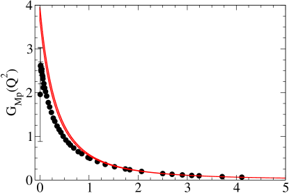
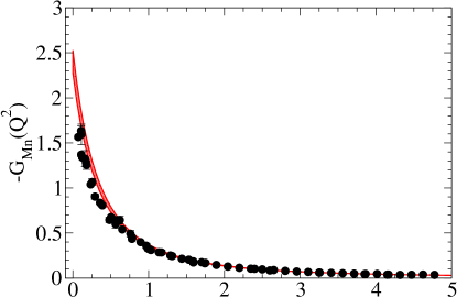
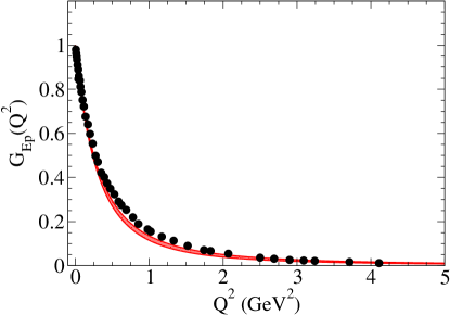
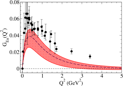
Figure 1: Proton and neutron electric and magnetic form factors for the parametrization from Table 1. The red band represents the interval between parametrization with $Q_{m}^{2}=1.5$ GeV² and $2.5$ GeV². In the case of $G_{En}$, the dashed-line represents the parametrization with $Q^{2}_{m}=2.0$ GeV². Data from Refs. ProtonData ; RefsGEn ; RefsGMn .

In an exact $SU(2)$-flavor model one has $\eta_{n}=-\eta_{p}$. These parameters can be determined by the proton and neutron bare anomalous magnetic moment $\kappa_{p}^{b}$ and $\kappa_{n}^{b}$ (we use the upper index $b$ to indicate the bare values). In a model with no meson cloud one can write $F_{2p}(0)\equiv\kappa_{p}=8\eta_{p}$ and $F_{2n}(0)\equiv\kappa_{n}=8\eta_{n}$, assuming $M_{N}=2\sqrt{2}\kappa$.

The holographic results (31)-(32) yield the correct perturbative QCD behavior for the nucleon electromagnetic form factors: $F_{1N}\propto 1/Q^{4}$ and $F_{2N}\propto 1/Q^{6}$, as consequence of $m=3/2$. Another observation about the current LF model and results (31)-(32) is that contrary to a common viewpoint on vector meson dominance in top-down holography, the number of poles contributing to the form factors is finite. This would not be the case, however, if a generic coupling $\hat{\mathcal{V}}$ is used in the overlap integral (18). For a more detailed discussion see Refs. Abidin09 ; Gutsche12a ; Gutsche13a ; inpreparation .

As previously discussed the couplings $\eta_{N}$ and $g_{V}$ are included phenomenologically. As can be seen from Eqs. (31)-(32), the minimal coupling only produces the Dirac form factor. The non-minimal couplings generate a non-zero $F_{2N}$ and adds an extra contribution to the Dirac form factor (proportional to $\eta_{N}$) Chakrabarti14a . Also the minimal-type coupling $g_{V}$ give a contribution for the Dirac form factor. Relations of the type (31)-(32) were derived for the first time in Ref. Abidin09 for the case $g_{V}=0$.

To determine the values of $g_{V}$ and $\eta_{N}$ we performed a fit to the data $Q^{2}\geq Q^{2}_{m}$ where $Q_{m}^{2}$ is the threshold of the data included in the fit. We considered the cases $Q^{2}_{m}=1.5$, 2.0 and 2.5 GeV², since the meson cloud effects are in principle suppressed for large $Q^{2}$, but we do not know a priory the threshold of the suppression. We use the data from Refs. ProtonData ; RefsGEn ; RefsGMn . Check Refs. Octet ; Medium for a detailed description of the database.

From the fits, we conclude that the results for the neutron electric form factor $G_{En}$ are very sensitive to the value of $Q_{m}^{2}$. If the low $Q^{2}$ is included in the fit ($Q^{2}_{m}<$ 1.0 GeV²) the best fit favors a negative $G_{En}$ for low $Q^{2}$, in conflict with the measured data. This result is very pertinent, because it is known that meson cloud effects, in particular the pion cloud, is very important for the description of the $G_{En}$ at low $Q^{2}$. Since the pion cloud contributions are not included in the parametrization of Eqs. (31)-(32), it is not surprising to see that the fit with $Q_{m}^{2}=1.5$ GeV² fails to describe the $G_{En}$ data. It can be surprising, however, to note that the best description of the nucleon data occurs for $Q^{2}>1.5$ GeV² in the fits with $Q_{m}^{2}=2.0$ and 2.5 GeV², when only a few data points for $G_{En}$ are considered. One then concludes that the shape of $G_{En}$ is determined by the form factors $G_{Ep}$, $G_{Mp}$ and $G_{Mn}$. This result shows the consistence of the fitting procedure.

The parameters obtained for the fits with $Q^{2}_{m}=1.5$, 2.0 and 2.5 GeV² are presented in Table 1. We can conclude that the parameters are sensitive to the data included in the fit. In particular, $g_{V}$ depends strongly of the threshold $Q_{m}^{2}$.

$Q_{m}^{2}$(GeV2)	$g_{V}$	$\eta_{p}$	$\eta_{n}$
1.5	1.571	0.378	$-$0.326
2.0	1.370	0.410	$-$0.345
2.5	1.275	0.424	$-$0.361

Table 1: Parameters $g_{V}$, $\eta_{p}$ and $\eta_{n}$ obtained by the fit of the nucleon form factor data with $Q^{2}\geq Q_{m}^{2}$.

The results obtained for the nucleon electric ($G_{EN}=F_{1N}-{\textstyle\frac{Q^{2}}{4M_{N}^{2}}}F_{2N}$) and magnetic ($G_{M\!N}=F_{1N}+F_{2N})$ form factors using the parameters from Table 1 are presented in Fig. 1. In the figure, we include a band to represent the interval between the models with $Q_{m}^{2}=1.5$ GeV² and $2.5$ GeV². In the calculations we used $\kappa=0.385$ GeV, in order to have a good description of the $\rho$ mesons and nucleon masses.

In general the estimates from different parametrizations are very close, except, for the neutron electric form factor. The function $G_{En}$ is in fact very sensitive to the parameters $g_{V}$, $\eta_{p}$ and $\eta_{n}$. In the graph of $G_{En}$ the lower limit corresponds to $Q_{m}^{2}=1.5$ GeV² and the upper limit to the case $Q_{m}^{2}=2.5$ GeV². The intermediate case ($Q_{m}^{2}=2.0$ GeV²) is included in order to emphasize the strong dependence of $G_{En}$ with the threshold $Q_{m}^{2}$ used in the fit, and it is represented by the dashed-line.

Concerning the remaining form factors, one can notice an overestimation of the low $Q^{2}$ data ($Q^{2}<1$ GeV²) for $G_{Mp}$ and $-G_{Mn}$. These results may be interpreted as the manifestation of the pion cloud effects, not included in the formalism associated with Eqs. (31)-(32).

In the past Gutsche12a ; Gutsche13a ; Chakrabarti14a the parameters $\eta_{N}$ and $g_{V}$ have been fixed by the static properties of the nucleon, such as the anomalous magnetic moments and the nucleon electric charge radius. Since those observables depend on the meson cloud, we choose in this work to fix the parameters in a region where the meson cloud is significantly reduced, in order to obtain a more accurate estimate of the bare parameters.

In the recent work the Brodsky-Teramond model for the nucleon Sufian17a was improved with the inclusion of the explicit pion cloud contributions ($q\bar{q}$ states) with a few adjustable parameters. It was shown that, indeed, the inclusion of the pion cloud contribution ($\tau=5$) is fundamental for an accurate description of $G_{En}$.

In order to understand the role of the valence quark degrees of freedom we restrict the present study to the the leading twist contribution ($\tau=3$). Once fixed the parameters of the model (bare parameters) one can use those parameters to calculate the valence quark contributions for the $\gamma^{\ast}N\to N(1440)$ transition form factors.

IV $\gamma^{\ast}N\to N(1440)$ form factors

We consider now the $\gamma^{\ast}N\to N(1440)$ transition form factors. Again omitting the spinors of the nucleon and the Roper (and the electric charge $e$), the transition current $J^{\mu}$ can be expressed as Roper

$$J^{\mu}=F_{1N}^{\ast}(Q^{2})\left(\gamma^{\mu}-\frac{{\not\!q}q^{\mu}}{q^{2}}\right)+F_{2N}^{\ast}(Q^{2})\frac{i\sigma^{\mu\nu}q_{\nu}}{M_{N}+M_{R}},$$

(33)

where $F_{1N}^{\ast}$ and $F_{2N}^{\ast}$ ($N=p,n$) are the Dirac and Pauli transition form factors, respectively.

Explicit analytical calculation, using the holographic wave functions (15) and (16) for the nucleon and the Roper, combined with the interaction (19), shows that the Dirac and Pauli form factors associated with the $\gamma^{\ast}N\to N(1440)$ in leading twist Gutsche13a are

$$F_{1N}^{\ast} = \delta_{N}\frac{a(\sqrt{2}a+c_{1})}{(a+1)(a+2)(a+3)(a+4)}+$$ (34)

$$g_{V}\delta_{N}\frac{a(\sqrt{2}a+c_{2})}{(a+1)(a+2)(a+3)(a+4)}+$$

$$\eta_{N}\frac{2a(2\sqrt{2}a^{2}-c_{3}a+c_{4})}{(a+1)(a+2)(a+3)(a+4)(a+5)},$$

$$F_{2N}^{\ast} = \eta_{N}\left(\frac{M_{R}+M_{N}}{M_{R}}\right)^{2}\frac{M_{R}}{2\sqrt{3}\kappa}$$ (35)

$$\times\frac{6\sqrt{3}(c_{5}a-4)}{(a+1)(a+2)(a+3)(a+4)},$$

where $c_{1}=4\sqrt{2}+3\sqrt{3}$, $c_{2}=4\sqrt{2}-3\sqrt{3}$, $c_{3}=9(\sqrt{3}-\sqrt{2})$, $c_{4}=3\sqrt{3}-5\sqrt{2}$ and $c_{5}=2+\sqrt{6}$.

In Eq. (35) we can replace ${\textstyle\frac{M_{R}}{2\sqrt{3}\kappa}}$ by unity if $2\sqrt{3}\kappa$ is a good approximation to the Roper mass. In the original form, Eqs. (34) and (35) were obtained in Ref. Gutsche13a . In comparison with that work we included an extra factor ${\textstyle\frac{M_{R}+M_{N}}{M_{R}}}$ in order to be consistent with the more usual definition of the transition form factors (33).

The results for the nucleon to Roper transition form factors associated with the parameters $g_{V}$, $\eta_{p}$ and $\eta_{n}$ discussed previously (Table 1), are presented in Fig. 2, for the proton target ($N=p$). As for the nucleon we use $\kappa=0.385$ GeV. The data presented here are those from CLAS/Jefferson Lab for single pion production CLAS1 and double pion production CLAS2 , and it is collected in the database MokeevDatabase . We do not discuss the results for the neutron target ($N=n$) because they are restricted to the photon point.

In Fig. 2, we can see that, contrary to the nucleon case, the results are almost insensitive to the variation of parameters, therefore we consider only the upper and lower cases ($Q_{m}^{2}=1.5$ and 2.5 GeV²), delimited by the band. In the figure one can see that the holographic approach based on Eqs. (34)-(35) in the leading twist approximation gives a very good description of the large $Q^{2}$ data ($Q^{2}>1.8$ GeV²) in the range $g_{V}=1.28$,…,1.57, $\eta_{p}=0.38$,…,0.42 and $\eta_{n}=-(0.36$,…,$0.32)$.

 

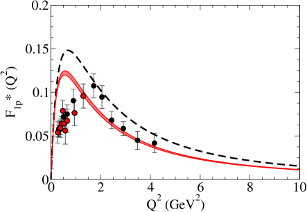
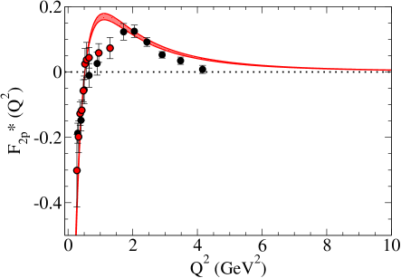
Figure 2: $\gamma^{\ast}N\to N(1440)$ transition form factors $F_{1p}^{\ast}$ and $F_{2p}^{\ast}$. The red band represents the interval between the models with $Q_{m}^{2}=1.5$ GeV² and $2.5$ GeV². The dashed-line is the result from the Light-Front holographic model from Ref. Teramond11a . Black dots from Ref. CLAS1 ; red dots from Ref. CLAS2 .

In the above holographic approach one obtains a clear estimate of the valence quark contributions based on framework that includes only one pre-defined parameter: the mass scale $\kappa$. Since the coefficients $g_{V}$, $\eta_{p}$, $\eta_{n}$ are determined by the nucleon form factors, one can consider this estimate of the valence quark contributions for the nucleon to Roper form factors as a parameter-free prediction.

The present results for $F_{1p}^{\ast}$ and $F_{2p}^{\ast}$ are consistent with estimates of the form factors based on different frameworks, such as the results of Refs. Aznauryan07 ; Roper ; Roper2 ; Segovia15 ; Aznauryan12b . In particular, the present model and the results of the covariant quark model from Refs. Nucleon ; Roper ; Roper2 are very close for $Q^{2}>5$ GeV².

The holographic calculation for the nucleon to Roper transition form factors given by Eqs. (34)-(35) were derived originally in Ref. Gutsche13a . In that work, higher Fock states (twist 4 and 5 contributions) were also taken into account. However the effective contribution of the higher Fock states was determined by the equation for the Roper mass, and not by the physics associated with the form factors (dominance of the leading twist contributions for large $Q^{2}$). In addition, the overlap between the nucleon and Roper states was determined in Ref. Gutsche13a using coefficients adjusted to the form factor data.

In the present work we rather prefer to concentrate on deriving a clean estimate of the valence quark contribution using an alternative method of fixing the parameters of the model, instead of trying to estimate the quark-antiquark and gluon contributions using LF holography. Since we do not consider higher twist contributions, the overlap between the states is just the result of the overlap between the valence quark states of both baryons with no unknown coefficients.

Although we conclude that the leading twist calculation is a good approximation for the form factors, one still notes that it may not be sufficient for a satisfactory estimate for the mass of the Roper. Different estimates of the mass suggest, in fact, that higher Fock states are crucial for the explanation of the experimental value Suzuki10 ; Capstick00 ; Gegelia16 .

In Fig. 2, we also present the first estimate of the the Dirac form factor, $F_{1p}^{\ast}$, performed by Teramond and Brodsky Teramond11a . In their formulation, the Dirac form factor is expressed by an analytic function dependent on the $\rho$ meson masses Brodsky15 ; Teramond11a ; Teramond12a . The closeness between results is a consequence of the use of the holographic masses instead of the physical masses. We note at this point, that, the relations (34)-(35) are also analytic parametrization of the Roper form factors, since the form factors are expressed in terms of functions of $a=\frac{Q^{2}}{m_{\rho}^{2}}$, using $m_{\rho}^{2}=4\kappa^{2}$. We leave however the comparison between analytic parametrization of the Roper form factors to a separated work newPaper .

In the graph for $F_{1p}^{\ast}$ one can notice a deviation between our estimate and the data for $Q^{2}<1$ GeV². This result can be interpreted as the consequence of the meson cloud contributions not included in our leading twist analysis. Similar results were obtained in independent works Aznauryan07 ; Roper ; Segovia15 . Sizable contributions of the meson cloud effects were found in Refs. Golli09 ; Obukhovsky11 .

As for the results for $F_{2p}^{\ast}$, one can note that the parametrization based on the LF holography gives negative values for small $Q^{2}$, and are close to the data. In particular we estimate the change of sign in $F_{2p}^{\ast}$ for $Q^{2}\approx 0.5$ GeV². The results for $F_{2p}^{\ast}$ suggest that contrarily to the form factor $F_{1p}^{\ast}$, where the meson cloud are sizable, for $F_{2p}^{\ast}$ the meson cloud contribution are very small at low $Q^{2}$. To the best of our knowledge, it is the first time that this fact was observed in the context of a quark model. There is, nevertheless, a discrepancy between the model and the data in the region between 0.9 and 1.5 GeV².

Concerning the $F_{2p}^{\ast}$ data, one can note that in the region 0.9–1.5 GeV² there are only two datapoints associated the two pion electroduction CLAS data CLAS2 . It is important to check if the new data associated with the one pion production confirms the trend from Ref. CLAS2 . At the moment one can conclude that the holographic model gives a very good description of the $F_{2p}^{\ast}$ data except for three data points in the range 0.9–1.5 GeV² (underestimation of the data in about 60%).

Discussion

Summarizing the results presented here for the nucleon and Roper form factors, one can conclude that the leading twist approximation provides a very good estimate for both nucleon and Roper form factors. This result is consistent with the LF formalism, because in the Drell-Yan-West frame the contributions from higher Fock states are small Brodsky08a ; Perdrisat07 ; Brodsky15 . It is expected however that the meson cloud effects provide significant contributions to the $\gamma^{\ast}N\to N^{\ast}$ transition form factors for some nucleon excitations $N^{\ast}$ for small $Q^{2}$ NSTAR ; S11 ; SQTM ; SemiRel ; NDelta-Lattice ; Delta1600 ; D13 ; DeltaQuad ; OctetDecuplet ; DeltaTL .

In the present work, the meson cloud effect is observed in particular for the form factors of the Roper: $F_{1p}^{\ast}$, and in the region 0.9–1.5 GeV² for $F_{2p}^{\ast}$. Those meson cloud corrections come from higher twist contributions to the Light-Front wave functions. For higher mass resonances it is expected that higher twist corrections also give important contributions to the transition form factors at low $Q^{2}$. In that case LF holography can be used to estimate mainly the contribution of the quark core. Although the estimate for low $Q^{2}$ may appear rough, since the calculation is based on massless quarks (and the physical quarks have mass), for large $Q^{2}$ the estimate is expected to be accurate due to the dominance of the valence quark degrees of freedom.

In the future one can use holography to estimate transition form factors in the leading twist approximation for other $N^{\ast}$ states. Those estimates are expected to be accurate at large $Q^{2}$, since they are based on valence quark degrees of freedom. At low $Q^{2}$ LF holography may fail in leading twist, since the framework provides only the valence quark contributions to the form factors. That information can be, however, very useful to understand the role of the meson cloud contributions. On one hand, we can use the comparison with the data to estimate the effect of the meson cloud contribution. On the other hand, estimates of the bare core can also be used as input to dynamical coupled-channel reaction models in the parametrization of baryon bare core Suzuki10 ; EBAC ; Burkert04 .

It is worth mentioning that some authors interpret the Roper as a dynamically-generated baryon-meson resonance, without an explicit reference to three-quark systems, except for the nucleon and the $\Delta(1232)$ Krehl00 ; Doring09 ; Liu16a ; Lang17 . As far as we know, there are no calculations of $\gamma^{\ast}N\to N(1440)$ transition form factors for intermediate and large $Q^{2}$, based on dynamically-generated resonance models for the Roper. Future lattice QCD simulations can help to understand the role of the baryon-meson contribution for the transition form factors at low $Q^{2}$ Liu16a ; Lang17 .

V Outlook and conclusions

In the present work we apply the LF holography in the soft-wall approximation to the study of the electromagnetic structure of the nucleon and nucleon excitations. More specifically we study the nucleon and $\gamma^{\ast}N\to N(1440)$ transition form factors in the leading twist approximation.

Since in the leading twist approximation the transition form factors are determined by the valence quark degrees of freedom, in the present approach we estimate the contribution of valence quarks to the electromagnetic form factors. The Light-Front wave functions are determined by an appropriate choice of boundary conditions in the 5D space and by the expected pQCD falloff for the Dirac and Pauli form factors (bottom-up approach to QCD).

The Light-Front holography in the soft-wall version was used previously in the study of the nucleon elastic form factors, in leading twist and higher orders. However, since in those works the couplings are adjusted to the dressed couplings (empirical anomalous magnetic moments) they may describe well the low $Q^{2}$ data, but fail in the description of the large-$Q^{2}$ data. In the present work we fix the free parameters of the model associated with the bare couplings using the large $Q^{2}$ data for the nucleon, where the effect of the meson cloud contributions is significantly reduced.

Our expressions for the electromagnetic form factors depend only of the holographic mass scale $\kappa$ and of three bare couplings: $g_{V}$, $\eta_{p}$ and $\eta_{n}$. Once determined the bare couplings by the nucleon data, the model is used to predict the $\gamma^{\ast}N\to N(1440)$ transition form factors.

Our results for the $\gamma^{\ast}N\to N(1440)$ transition form factors compare well with the empirical data. For the Dirac form factor, the deviation observed for $Q^{2}<1.0$ GeV² is compatible with the interpretation that meson cloud contributions are important in that region. As for the Pauli form factor, our estimate is very close to the data, both at low and at large $Q^{2}$, except for 3 datapoints in the range 0.9–1.5 GeV². The result at low $Q^{2}$, suggests that the meson cloud contributions for $F_{2p}^{\ast}$ are small. As far as we know this is the first time that this effect is observed.

The method used in the present work for the Roper can in the future be extended for higher mass nucleon excitations. The use of the Light-Front holography in leading twist provides then a natural method to estimate the valence quark contributions for the transition form factors. The effect of the meson cloud can then be estimated from the comparison with the experimental data.

Theoretical estimates of the bare core contributions are very important for the study of the baryon-meson reactions and nucleon electroproduction reactions. The results from Light-Front holography may be used as input to dynamical coupled-channel reaction models in the theoretical study of those reactions.