Quantum analysis of fluctuations of electromagnetic fields in heavy-ion collisions

Abstract

We perform quantum calculations of fluctuations of the electromagnetic fields in $AA$ collisions at RHIC and LHC energies. The analysis is based on the fluctuation-dissipation theorem. We find that in the quantum picture the field fluctuations are very small. They turn out to be much smaller than the predictions of the classical Monte-Carlo simulation with the Woods-Saxon nuclear density.

Introduction. Non-central heavy ion collisions at RHIC and LHC energies should generate a very strong magnetic field perpendicular to the reaction plane Kharzeev_B1 ; Toneev_B1 . At the initial moment it can reach the values up to $eB\sim 3m_{\pi}^{2}$ for RHIC ($\sqrt{s}=0.2$ TeV) and a factor of 15 bigger for LHC ($\sqrt{s}=2.76$ TeV) Kharzeev_B1 ; Toneev_B1 ; Tuchin_B ; Z_maxw . The presence of the magnetic field may lead to charge separation along the magnetic field direction due to the anomalous current $\propto{{\bf B}}$ (the Chiral Magnetic Effect (CME)) in the quark-gluon plasma (QGP) produced in the initial stage of $AA$ collisions Kharzeev_B1 ; Kharzeev_CME_rev . The effect is supported by the experimental data on the charged particle correlations STAR_CME . But the situation remains somewhat unclear due to non-CME related background effects Kharzeev_report .

An important issue arising in the context of the CME and charge separation in $AA$ collisions concerns fluctuations of the magnetic field. They partly destroy the correlation between the magnetic field direction and the reaction plane, and can lead to reduction of the ${{\bf B}}$-induced observables Liao_MC . Fluctuations of the electromagnetic fields in $AA$ collisions have been addressed in several studies Skokov_MC ; Deng_MC ; Liao_MC by Monte-Carlo (MC) simulation with the Woods-Saxon (WS) nuclear distribution using the classical Lienard-Weichert potentials. The results of Skokov_MC ; Deng_MC ; Liao_MC show that fluctuating proton positions lead to considerable event-by-event fluctuations of the magnetic field both parallel and perpendicular to the reaction plane. It would be highly desirable to perform a quantum analysis of the problem. Because the classical treatment has no theoretical justification. Indeed, the dominating contribution to fluctuations of the electromagnetic fields is connected with fluctuations of the nuclear dipole moments. It is well known that the nuclear dipole fluctuations are dominated by the giant dipole resonance (GDR), which is a collective excitation closely related to the symmetry energy of the nuclear matter Greiner ; Speth ; Trippa . But in the description of nuclei in terms of the factorized WS nuclear distribution this collective quantum dynamics of the nuclear ground state is completely ignored. The classical treatment of the electromagnetic field in the problem of interest may also be inadequate. Because, similarly to calculations of the van der Waals forces Casimir , it becomes invalid at large distances.

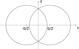
Figure 1: The transverse plane of a non-central $AA$ collision with the impact parameter $b$.

In the present letter we perform a quantum analysis of the field fluctuations in $AA$ collisions at RHIC and LHC energies. Our framework is based on the general formulas of the fluctuation-dissipation theorem Callen for the electromagnetic fluctuations in the form given in LL9 . This formalism allows to express the field fluctuations in $AA$ collisions via the nuclear dipole polarizability.

Theoretical framework. We consider the proper time region $\tau\sim 0.2-1$ fm which is of the most interest from the point of view of the ${{\bf B}}$-induced effects in the QGP. Because in this time region the QGP may be already present, and the magnetic field is still significant. The MC simulation of the electromagnetic fields in $AA$ collisions using the retarded Lienard-Weichert potentials show that almost all contribution to the electromagnetic field comes from the currents generated by the fast protons in the space-time region before intersection of the nuclear disks. For this reason one can ignore the effect of interaction of the colliding nuclei on the currents from the participant protons involved in the nuclear collision. In any case, for the RHIC and LHC energies, a possible change of the fast quark currents at the time scale $t\mathrel{\hbox to0.0pt{\lower 4.0pt\hbox{\hskip 1.0pt$\sim$}\hss}\raise 1.0pt\hbox{$<$}}1$ fm should be very small. We make a reasonable assumption that, similarly to the classical case, in the quantum picture the effect of the electric currents from the fast protons in the stage after the nuclear collision is negligible. In the present analysis we ignore the electromagnetic fields generated in the QGP stage by new quarks and antiquarks produced after interaction of the Lorentz contracted colliding nuclei Skokov_B ; Tuchin_B ; Z_maxw . Then the problem is reduced to evaluating the electromagnetic fields generated by two colliding nuclei in the ground state.

We consider two colliding nuclei (right moving and left moving) with velocities ${{\bf V}}_{R}=(0,0,V)$ and ${{\bf V}}_{L}=(0,0,-V)$, and with the impact parameters ${{\bf b}}_{R}=(0,-b/2)$ and ${{\bf b}}_{L}=(0,b/2)$ (as shown in Fig. 1). We take $z_{R,L}=\pm Vt$. The electromagnetic field from each nucleus is a sum of the mean field and the fluctuating field

$$F^{\mu\nu}=\langle F^{\mu\nu}\rangle+\delta F^{\mu\nu}\,.$$ (1)

For each nucleus $\langle{{\bf E}}\rangle$ and $\langle{{\bf B}}\rangle$ are given by the Lorentz transformation of its Coulomb field in the nucleus rest frame. For a nucleus with velocity ${{\bf V}}=(0,0,V)$ and the impact vector ${{\bf b}}$ the mean electric and magnetic fields at $x^{\mu}=(t,\mbox{{\boldmath$\rho$}},z)$ read

$$\langle{{\bf E}}_{T}(t,\mbox{{\boldmath$\rho$}},z)\rangle=\gamma\frac{E_{A}(r^{\prime})(\mbox{{\boldmath$\rho$}}-{{\bf b}})}{r^{\prime}}\,,$$ (2)

$$\langle E_{z}(t,\mbox{{\boldmath$\rho$}},z)\rangle=\frac{E_{A}(r^{\prime})z^{\prime}}{r^{\prime}}\,,$$ (3)

$$\langle{{\bf B}}(t,\mbox{{\boldmath$\rho$}},z)\rangle=[{{\bf V}}\times\langle{{\bf E}}(t,\mbox{{\boldmath$\rho$}},z)\rangle]\,.$$ (4)

Here $\gamma=1/\sqrt{1-V^{2}}$ is the Lorentz factor, $r^{\prime 2}=(\mbox{{\boldmath$\rho$}}-{{\bf b}})^{2}+z^{\prime 2}$, $z^{\prime}=\gamma(z-Vt)$, and

$$E_{A}(r)=\frac{4\pi}{r^{2}}\int_{0}^{r}d\xi\xi^{2}\rho_{A}(\xi)$$ (5)

is the electric field of the nucleus in its rest frame, $\rho_{A}$ is the nucleus charge density. From (2)–(5) one can obtain that for two colliding nuclei the mean magnetic field at $\mbox{{\bf r}}=0$ has only $y$-component. At $t^{2}\mathrel{\hbox to0.0pt{\lower 4.0pt\hbox{\hskip 1.0pt$\sim$}\hss}\raise 1.0pt\hbox{$>$}}(R_{A}^{2}-b^{2}/4)/\gamma^{2}$ (here $R_{A}$ is the nucleus radius, and $b$ is assumed to be $<2R_{A}$) it is approximately

$$\langle B_{y}(t,\mbox{{\bf r}}=0)\rangle\approx\frac{\gamma Zeb}{(b^{2}/4+\gamma^{2}V^{2}t^{2})^{3/2}}\,.$$ (6)

At $t\gg R_{A}/\gamma$ in the region $\rho\ll t\gamma$ $\langle B_{y}(t,\mbox{{\boldmath$\rho$}},z=0)\rangle$ takes a simple $\rho$-independent form

$$\langle B_{y}(t,\mbox{{\boldmath$\rho$}},z=0)\rangle\approx Zeb/\gamma^{2}t^{3}\,.$$ (7)

The contribution of each nucleus to the correlators of the electromagnetic fields in the lab-frame may be expressed via the correlators in the nucleus rest frame. For $\gamma\gg 1$ the dominating fluctuations in the lab-frame are the ones of the transverse fields. The transverse components of the correlators of the electric and magnetic fields can be written as

$$\langle\delta E_{i}\delta E_{k}\rangle=\gamma^{2}\left[\langle\delta E_{i}\delta E_{k}\rangle+V^{2}e_{3il}e_{3kj}\langle\delta B_{l}\delta B_{j}\rangle\right]_{rf},$$ (8)

$$\langle\delta B_{i}\delta B_{k}\rangle=\gamma^{2}\left[\langle\delta B_{i}\delta B_{k}\rangle+V^{2}e_{3il}e_{3kj}\langle\delta E_{l}\delta E_{j}\rangle\right]_{rf},$$ (9)

where $i,k$ are the transverse indices and the subscript $rf$ on the right-hand side of (8), (9) indicates that the correlators are calculated in the nucleus rest frame.

In calculations of the rest frame correlators $\langle\delta E_{l}\delta E_{j}\rangle$, $\langle\delta B_{i}\delta B_{k}\rangle$ (hereafter we drop the subscript $rf$) with the help of the FDT we follow the formalism of LL9 (formulated in the gauge $\delta A^{0}=0$). It allows to relate the time Fourier component of the vector potential correlator

$$\langle\delta A_{i}(\mbox{{\bf r}}_{1})\delta A_{k}(\mbox{{\bf r}}_{2})\rangle_{\omega}=\frac{1}{2}\int dte^{i\omega t}\langle\delta A_{i}(t,\mbox{{\bf r}}_{1})\delta A_{k}(0,\mbox{{\bf r}}_{2})$$

$$+\delta A_{k}(0,\mbox{{\bf r}}_{2})\delta A_{i}(t,\mbox{{\bf r}}_{1})\rangle\hskip 56.9055pt$$ (10)

and that of the retarded Green’s function

$$D_{ik}(\omega,\mbox{{\bf r}}_{1},\mbox{{\bf r}}_{2})=-i\int dte^{i\omega t}\theta(t)\langle\delta A_{i}(t,\mbox{{\bf r}}_{1})\delta A_{k}(0,\mbox{{\bf r}}_{2})$$

$$-\delta A_{k}(0,\mbox{{\bf r}}_{2})A_{i}(t,\mbox{{\bf r}}_{1})\rangle\,.\hskip 56.9055pt$$ (11)

In the zero temperature limit the FDT relation between (10) and (11) reads LL9

$$\!\!\langle\delta A_{i}(\mbox{{\bf r}}_{1})\delta A_{k}(\mbox{{\bf r}}_{2})\rangle_{\omega}\!=\!-\mbox{sign}(\omega)\mbox{Im}D_{ik}(\omega,\mbox{{\bf r}}_{1},\mbox{{\bf r}}_{2}).$$ (12)

The time Fourier components of the electromagnetic field correlators in terms of that for the the vector potential correlator (10) are given by

$$\langle\delta E_{i}(\mbox{{\bf r}}_{1})\delta E_{k}(\mbox{{\bf r}}_{2})\rangle_{\omega}=\omega^{2}\langle\delta A_{i}(\mbox{{\bf r}}_{1})\delta A_{k}(\mbox{{\bf r}}_{2})\rangle_{\omega}\,,$$ (13)

$$\langle\delta B_{i}(\mbox{{\bf r}}_{1})\delta B_{k}(\mbox{{\bf r}}_{2})\rangle_{\omega}=\mbox{rot}^{(1)}_{il}\mbox{rot}^{(2)}_{kj}\langle\delta A_{l}(\mbox{{\bf r}}_{1})\delta A_{j}(\mbox{{\bf r}}_{2})\rangle_{\omega}.$$ (14)

The same point field correlators that we need read

$$\langle\delta E_{i}(t,\mbox{{\bf r}})\delta E_{k}(t,\mbox{{\bf r}})\rangle=\frac{1}{2\pi}\int_{-\infty}^{\infty}d\omega\langle\delta E_{i}(\mbox{{\bf r}})\delta E_{k}(\mbox{{\bf r}})\rangle_{\omega}\,,$$ (15)

$$\langle\delta B_{i}(t,\mbox{{\bf r}})\delta B_{k}(t,\mbox{{\bf r}})\rangle=\frac{1}{2\pi}\int_{-\infty}^{\infty}d\omega\langle\delta B_{i}(\mbox{{\bf r}})\delta B_{k}(\mbox{{\bf r}})\rangle_{\omega}\,.$$ (16)

In the time region of interest $t\mathrel{\hbox to0.0pt{\lower 4.0pt\hbox{\hskip 1.0pt$\sim$}\hss}\raise 1.0pt\hbox{$>$}}0.2$ fm (in the lab-frame) in (15), (16) for each nucleus the distance between the observation point r and the center of the nucleus (in its rest frame) is much bigger than $R_{A}$. In this regime one may treat each nucleus as a point like dipole described by the dipole polarizability $\alpha_{ik}(\omega)$ (in the sense of the fluctuating field components). In the formalism of LL9 the field fluctuations are described by correction to the retarded Green’s function proportional to the dipole polarizability. The retarded Green’s function coincides with the Green’s function of Maxwell’s equation LL9 . In the presence of the point like dipole at $\mbox{{\bf r}}=\mbox{{\bf r}}_{A}$ the equation determining the retarded Green’s function reads

$$\left[\frac{\partial^{2}}{\partial x_{i}\partial_{l}}-\delta_{il}\triangle-\delta_{il}\omega^{2}-4\pi\omega^{2}\alpha_{il}(\omega)\delta(\mbox{{\bf r}}-\mbox{{\bf r}}_{A})\right]$$

$$\times D_{lk}(\omega,\mbox{{\bf r}},\mbox{{\bf r}}^{\prime})=-4\pi\delta_{ik}\delta(\mbox{{\bf r}}-\mbox{{\bf r}}^{\prime})\,.\hskip 28.45274pt$$ (17)

The correction to $D_{ik}$ due to $\alpha_{ik}$ reads LL9

$$\Delta D_{ik}(\omega,\mbox{{\bf r}}_{1},\mbox{{\bf r}}_{2})=-\omega^{2}D_{il}^{v}(\omega,\mbox{{\bf r}}_{1},\mbox{{\bf r}}_{A})\alpha_{lm}(\omega)$$

$$\times D_{mk}^{v}(\omega,\mbox{{\bf r}}_{A},\mbox{{\bf r}}_{2})\,.$$ (18)

Here $D_{ik}^{v}$ is the vacuum Green’s function that is given by

$$D_{ik}^{v}(\omega,\mbox{{\bf r}}_{1},\mbox{{\bf r}}_{2})=\delta_{ik}D_{1}(\omega,r)+\frac{x_{i}x_{k}}{r^{2}}D_{2}(\omega,r)\,,$$ (19)

where $\mbox{{\bf r}}=\mbox{{\bf r}}_{1}-\mbox{{\bf r}}_{2}$, and

$$D_{1}(\omega,r)=-\frac{e^{i\omega r}}{r}\left(1+\frac{i}{\omega r}-\frac{1}{\omega^{2}r^{2}}\right)\,,$$ (20)

$$D_{2}(\omega,r)=\frac{e^{i\omega r}}{r}\left(1+\frac{3i}{\omega r}-\frac{3}{\omega^{2}r^{2}}\right)\,.$$ (21)

For spherical nuclei the polarizability tensor can be written as $\alpha_{ik}(\omega)=\delta_{ik}\alpha(\omega)$. $\alpha(\omega)$ is an analytical function of $\omega$ in the upper half-plane LL4 . It satisfies the relation $\alpha^{*}(-\omega^{*})=\alpha(\omega)$ LL4 It means that on the upper imaginary axis $\alpha(\omega)$ is real. Using this fact, from Eqs. (18)–(21) one can obtain for the rest frame field correlators (we take $\mbox{{\bf r}}_{A}=0$)

$$\langle\delta E_{i}(t,\mbox{{\bf r}})\delta E_{k}(t,\mbox{{\bf r}})\rangle=\delta_{ik}J_{1}(r)+\frac{x_{i}x_{k}}{r^{2}}J_{2}(r)\,,$$ (22)

$$\langle\delta B_{i}(t,\mbox{{\bf r}})\delta B_{k}(t,\mbox{{\bf r}})\rangle=\left(\delta_{ik}-\frac{x_{i}x_{k}}{r^{2}}\right)J_{3}(r)\,,$$ (23)

where

$$J_{1}=\frac{1}{2\pi r^{7}}\left[I_{0}+I_{1}+\frac{3}{4}I_{2}+\frac{1}{4}I_{3}+\frac{1}{16}I_{4}\right]\,,$$ (24)

$$J_{2}=\frac{1}{2\pi r^{7}}\left[3I_{0}+3I_{1}+\frac{1}{4}I_{2}-\frac{1}{4}I_{3}-\frac{1}{16}I_{4}\right]\,,$$ (25)

$$J_{3}=-\frac{1}{8\pi r^{7}}\left[I_{2}+I_{3}+\frac{1}{4}I_{4}\right]\,,$$ (26)

$$I_{n}=\int_{0}^{\infty}d\xi\xi^{n}e^{-\xi}\alpha\left(\frac{i\xi}{2r}\right)\,.$$ (27)

These formulas allow to express the fluctuations of the electromagnetic fields of each nuclei via the dipole polarizability $\alpha(\omega)$.

Parametrization of the dipole polarizability. The function $\alpha(\omega)$ reads LL4 ; Migdal_GDR

$$\alpha(\omega)=\frac{1}{3}\sum_{s}\left[\frac{|\langle 0|{{\bf d}}|s\rangle|^{2}}{\omega_{s0}-\omega-i\delta}+\frac{|\langle 0|{{\bf d}}|s\rangle|^{2}}{\omega_{s0}+\omega+i\delta}\right]\,,$$ (28)

where ${{\bf d}}$ is the dipole operator

$${{\bf d}}=e\frac{N}{A}\sum_{p}\mbox{{\bf r}}_{p}-e\frac{Z}{A}\sum_{n}\mbox{{\bf r}}_{n}\,.$$ (29)

At $\omega>0$ the dipole polarizability tensor coincides with the photon scattering tensor LL4 . This allows to express the imaginary part of $\alpha(\omega)$ in terms of the dipole photoabsorption cross section as

$$\sigma_{abs}(\omega)=4\pi\omega\mbox{Im}\alpha(\omega)\,.$$ (30)

For heavy nuclei the dipole strength is dominated by the GDR Greiner ; GDR_RMP75 ; Speth . It appears as a broad peak in the $\sigma_{abs}$ with a mean energy $\sim 14$ MeV GDR_RMP75 . We parametrize the dipole polarizability for ¹⁹⁷Au and ²⁰⁸Pb nuclei by a single GDR state

$$\alpha(\omega)=c\left[\frac{1}{\omega_{10}-\omega-i\Gamma/2}+\frac{1}{\omega_{10}+\omega+i\Gamma/2}\right]\,.$$ (31)

By fitting the data on the photoabsorption cross section from GDR_Au for ¹⁹⁷Au and from GDR_Pb for ²⁰⁸Pb we obtained the following values of the parameters: $\omega_{10}\approx 13.6$ MeV, $\Gamma\approx 4.38$ MeV, $c\approx 18.2$ GeV^-2 for ¹⁹⁷Au, and $\omega_{10}\approx 13.3$ MeV, $\Gamma\approx 3.72$ MeV, $c\approx 18.93$ Gev^-2 for ²⁰⁸Pb.

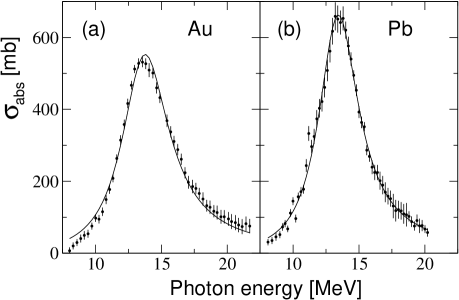
Figure 2: Fit of the photoabsorption cross section in the GDR region to the experimental data for ¹⁹⁷Au and ²⁰⁸Pb targets. The data are from Refs. GDR_Au and GDR_Pb , respectively.

Fig. 2 illustrates the quality of our fit.

Results and Discussion. The fluctuations of the electromagnetic fields occur due to the fluctuations of the nuclear dipole moment. For this reason, it is interesting to begin with comparison of the dipole moment fluctuations in the quantum and the classical models. In the quantum model from (28), (31) one can obtain

$$\langle 0|{{\bf d}}^{2}|0\rangle=\frac{3}{\pi}\int_{0}^{\infty}d\omega\mbox{Im}\alpha(\omega)=\frac{6c}{\pi}\mbox{arctg}\left(2\omega_{10}/\Gamma\right)\,.$$ (32)

This formula with parameters fitted to the data on $\sigma_{abs}$ gives $\langle 0|{{\bf d}}^{2}|0\rangle\approx 1.91$ fm² and $\langle 0|{{\bf d}}^{2}|0\rangle\approx 2.02$ fm² for ¹⁹⁷Au and ²⁰⁸Pb nuclei, respectively. The classical MC calculation with the WS nuclear density gives for these nuclei the values $\langle{{\bf d}}^{2}\rangle\approx 9.89$ fm² and $\langle{{\bf d}}^{2}\rangle\approx 10.39$ fm². One sees that the classical treatment overestimates the dipole moment squared by a factor of $\sim 5$.

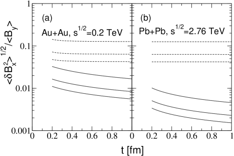
Figure 3: The $t$-dependence of the ratio $\langle\delta B_{x}^{2}\rangle^{1/2}/\langle B_{y}\rangle$ at $\mbox{{\bf r}}=0$ for Au+Au collisions at $\sqrt{s}=0.2$ TeV (left) and for Pb+Pb collisions at $\sqrt{s}=2.76$ TeV for different impact parameters $b=3$, $6$ and $9$ fm (from top to bottom). Solid lines are for quantum calculations, dashed lines for classical MC calculations with the WS nuclear density.

The fluctuations of the direction of the magnetic field at the center of the plasma fireball are dominated by the fluctuations of the component $B_{x}$ that vanishes without fluctuations. In Fig. 3 we confront our quantum and classical results for $t$-dependence of the ratio $\langle\delta B_{x}^{2}\rangle^{1/2}/\langle B_{y}\rangle$ at $x=y=0$. This ratio gives the typical angle between the magnetic field and the perpendicular to the reaction plane. The results are shown for the impact parameters $b=3,$ $6$ and $9$ fm for Au+Au collisions at $\sqrt{s}=0.2$ TeV and Pb+Pb collisions at $\sqrt{s}=2.76$ TeV. One can see that the quantum calculations give $\langle\delta B_{x}^{2}\rangle^{1/2}/\langle B_{y}\rangle$ smaller than the classical ones by a factor of $\sim 5-8$ for RHIC and by a factor of $\sim 13-27$ for LHC. This difference results from both the reduction of the nuclear dipole moment fluctuations in the quantum picture and from the quantum effects for the electromagnetic field (that are especially important for the LHC energy). We have presented the results for the magnetic field. The results for fluctuations of the transverse electric field at $\mbox{{\bf r}}=0$ are close to that for the magnetic field (recall that $\langle E_{x,y}\rangle=0$ at $\mbox{{\bf r}}=0$).

Thus we see that in the quantum picture both for RHIC and LHC fluctuations of the direction of the magnetic field relative to the reaction plane are very small. Of course, in event-by-event measurements the reaction plane itself cannot be determined exactly. Experimentally the orientation of the reaction plane is extracted from the elliptic flow in the particle distribution Ollitrault_v2 ; Voloshin_v2 , and it fluctuates around the real reaction plane. This plane extracted from the data is often called the participant plane. In the hydrodynamical picture of the QGP evolution calculations of the fluctuations of the direction of the magnetic field to the participant plane require a joint analysis of the field fluctuations and of the fluctuations of the initial entropy deposition. The latter control the fluctuations of the orientation of the participant plane. The initial entropy deposition is sensitive to the long range fluctuations in the nuclear density. One of the types of the collective nuclear modes that can be important is the fluctuations related to the GDR. But another collective modes such as the giant monopole resonance (corresponding to spherically symmetric nuclear oscillations) and the giant quadruple resonance Greiner may also be important for the participant plane fluctuations. Our analysis shows that for the dipole mode the classical treatment based on the MC simulation with the WS nuclear density overestimates the fluctuations. It would be of great interest to clarify the situation for other collective modes. In particular, this is of great interest for the event-by-event hydrodynamic simulations of $AA$ collision. All this, however, is far beyond of the scope of the present work.

Conclusion. In this work within the FDT formalism of LL9 we have performed a quantum analysis of fluctuations of the electromagnetic field in $AA$ collisions at RHIC and LHC energies. Our quantum calculations show that the field fluctuations are very small, and they practically do not affect the direction of the magnetic field as compared to the mean field classical predictions. By confronting our quantum results with that from the classical MC simulation with the WS nuclear distribution, we have demonstrated that the classical picture overestimates strongly the field fluctuations. Our results are in contradiction with the conclusion of the recent analysis Tuchin_quantum , where it was argued that the quantum diffusion of the protons may be very important. However, the analysis Tuchin_quantum is performed for free particles, and the results are inapplicable directly to nuclei in the ground state.

- (1) D.E. Kharzeev, L.D. McLerran, and H.J. Warringa, Nucl. Phys. A803, 227 (2008) [arXiv:0711.0950].
- (2) V. Skokov, A.Yu. Illarionov, and V. Toneev, Int. J. Mod. Phys. A24, 5925 (2009) [arXiv:0907.1396].
- (3) K. Tuchin, Phys. Rev. C88, 024911 (2013) [arXiv:1305.5806].
- (4) B.G. Zakharov, Phys. Lett. B737, 262 (2014) [arXiv:1404.5047].
- (5) D.E. Kharzeev, Prog. Part. Nucl. Phys. 75, 133 (2014) [arXiv:1312.3348].
- (6) B.I. Abelev et al. [STAR Collaboration], Phys.Rev. C81, 054908 (2010) [arXiv:0909.1717].
- (7) D.E. Kharzeev, J. Liao, and S.A. Voloshin, Prog. Part. Nucl. Phys. 88, 1 (2016) [arXiv:1511.04050].
- (8) J. Bloczynski, X.-G. Huang, X. Zhang, and J. Liao, Phys. Lett. B718, 1529 (2013) [arXiv:1209.6594].
- (9) A. Bzdak and V. Skokov, Phys. Lett. B710, 171 (2012) [arXiv:1111.1949].
- (10) W.-T. Deng and X.-G. Huang, Phys. Rev. C85, 044907 (2012) [arXiv:1201.5108].
- (11) W. Greiner and J.A. Maruhn, Nuclear models, Berlin, Springer, 1996.
- (12) S. Kamerdzhiev, J. Speth, and G. Tertychny, Phys. Rept. 393, 1 (2004) [nucl-th/0311058].
- (13) L. Trippa, G. Colo, and E. Vigezzi, Phys. Rev. C77, 061304 (2008) [arXiv:0802.3658].
- (14) H.B.G. Casimir and D. Polder, Phys. Rev. 73, 360 (1948).
- (15) H.B. Callen and T.A. Welton, Phys. Rev. 83, 34 (1951).
- (16) E.M. Lifshits and L.P. Pitaevski, Statistical Physics, Part 2 (Landau Course of Theoretical Physics Vol. 9), Oxford, Pergamon Press, 1980.
- (17) L. McLerran and V. Skokov, Nucl. Phys. A929, 184 (2014) [arXiv:1305.0774].
- (18) V.B. Berestetski, E.M. Lifshits, and L.P. Pitaevski, Quantum Electrodynamics (Landau Course of Theoretical Physics Vol. 4), Oxford, Pergamon Press, 1979.
- (19) A.B. Migdal, A.A. Lushnikov, and D.F. Zaretsky, Nucl. Phys. 66, 193 (1965).
- (20) B.L. Berman and S.C. Fultz, Rev. Mod. Phys. 47, 713 (1975).
- (21) A. Veyssiere, H. Beil, R. Bergere, P. Carlos, and A. Lepretre, Nucl. Phys. A159, 561 (1970).
- (22) A. Tamii et al., Phys. Rev. Lett. 107, 062502 (2011) [arXiv:1104.5431].
- (23) J.-Y. Ollitrault, Phys. Rev. D46, 229 (1992).
- (24) S. Voloshin and Y. Zhang, Z. Phys. C70, 665 (1996) [hep-ph/9407282].
- (25) R. Holliday, R. McCarty, B. Peroutka, and K. Tuchin, Nucl. Phys. A957, 406 (2017) [arXiv:1604.04572].