Statistical properties of one-dimensional directed polymers in a random potential

Abstract

This review is devoted to the detailed consideration of the universal statistical properties of one-dimensional directed polymers in a random potential. In terms of the replica Bethe ansatz technique we derive several exact results for different types of the free energy probability distribution functions. In the second part of the review we discuss the problems which are still waiting for their solutions. Several mathematical appendices in the ending part of the review contain various technical details of the performed calculations.

Contents

	I.	Introduction	……..1
	II.	Replica method	……..3
	III.	Mapping to quantum bosons	……..6
		Part 1: Exact results
	IV.	GUE Tracy-Widom distribution in the model with fixed boundary conditions	……..10
		A. Generating function approach	……..10
		B. Inverse Laplace transformation approach	……..12
	V.	GOE Tracy-Widom distribution in the model with free boundary conditions	……..14
	VI.	Multi-point free energy distribution functions	……..21
		A. Two-point distribution	……..21
		A. $N$-point distribution	……..26
	VII.	Probability distribution function of the endpoint fluctuations	……..32
		Part 2: Unsolved problems
	VIII.	Zero temperature limit	……..38
	IX.	Random force Burgers turbulence	……..43
	X.	Joint distribution function of free energies at two different temperatures	……..52
	XI	Conclusions	……..57
	Appendix A: GUE Tracy-Widom distribution function		……..58
	Appendix B: The Airy function integral relations		……..59
	Appendix C: Fredholm determinant with the Airy kernel		……..60
	Appendix D: Useful combinatorial identities		……..63
	Appendix E: Technical part of Chapter V		……..64

I Introduction

It is well known that macroscopic characteristics of any random system defined in terms of macroscopic number of independent random parameters (according to the central limit theorem) are described by the Gaussian distribution function. In a sense, such type of the universal behavior is trivial, and not so much interesting. On the other hand, any non-trivial system usually requires individual consideration, and although there are lot of universal macroscopic properties among microscopically different systems (e.g. scaling and critical phenomena at the phase transitions) until very recently no one would expect to have a universal function (different from the Gaussian one) which would describe macroscopic statistical properties of a whole class of non-trivial random systems.

One of the main achievement of the last three decades in the scope of the disordered systems is the discovery of the entire class of random systems whose macroscopic properties are described by the same universal probability distribution function which is called the Tracy-Widom (TW) distribution TW-GUE . Traditionally it is called the KPZ universality class by the name of the celebrated Kardar-Parisi-Zang equation KPZ which describes the time evolution of an interface (separating two homogeneous bulk phases) in the disordered inhomogeneous media.

Originally the solution of Tracy and Widom TW-GUE were devoted to rather specific mathematical problem, namely the distribution function of the largest eigenvalue of $N\times N$ Hermitian matrices (Gaussian Unitary Ensemble (GUE)) in the limit $N\to\infty$. Nowadays we have got rather comprehensive list of various systems (both purely mathematical and physical) whose macroscopic statistical properties are described by the same universal TW distribution function. Among these systems are: the longest increasing subsequences (LIS) model LIS ; zero-temperature lattice directed polymers with geometric disorder DP_johansson ; the polynuclear growth (PNG) system PNG_Spohn ; the oriented digital boiling model oriented_boiling ; the ballistic decomposition model ballistic_decomposition1 ; ballistic_decomposition2 ; the longest common subsequences (LCS) LCS ; the fixed-trace ensembles of random matrices fixed-trace-ensembles the asymmetric simple exclusion process (ASEP)ASEP1 ; ASEP2 ; ASEP3 ; etc. Besides, there are lot of physical and biological systems in which the KPZ universality class scaling behavior has been convincingly demonstrated experimentally: bacterial colony growth bacteria ; paper combustion paper ; liquid-crystal electroconvection liquid-crystal ; eucariotic cell colony growth eucariotic ; particle decomposition in coffee rings coffe ; chemical reaction front chemical-reaction (see also exper-rev for a review on experiments).

In this review we are going to concentrate on the model of directed polymers defined in terms of an elastic string $\phi(\tau)$ directed along the $\tau$-axes within an interval $[0,t]$ which passes through a random medium described by a random potential $V(\phi,\tau)$. The energy of a given polymer’s trajectory $\phi(\tau)$ is

$$H[\phi(\tau);V]=\int_{0}^{t}d\tau\Bigl{\{}\frac{1}{2}\bigl{[}\partial_{\tau}\phi(\tau)\bigr{]}^{2}+V[\phi(\tau),\tau]\Bigr{\}};$$ (1.1)

Here the disorder potential $V[\phi,\tau]$ is supposed to be Gaussian distributed with a zero mean $\overline{V(\phi,\tau)}=0$ and the $\delta$-correlations

$${\overline{V(\phi,\tau)V(\phi^{\prime},\tau^{\prime})}}=u\delta(\tau-\tau^{\prime})\delta(\phi-\phi^{\prime})$$ (1.2)

where $\overline{(...)}$ denotes the disorder average and the parameter $u$ describes the strength of the random potential. Diverse physical systems such as domain walls in magnetic films lemerle_98 , vortices in superconductors blatter_94 , wetting fronts on planar systems wilkinson_83 , or Burgers turbulence burgers_74 ; turbulence can be mapped to this model, which exhibits numerous non-trivial features deriving from the interplay between elasticity and disorder.

The system defined by the above Hamiltonian (1.1) has been the subject of intense investigations during the past almost three decades (see e.g. hh_zhang_95 ; kardar_book ; hhf_85 ; numer1 ; numer2 ; kardar_87 ; bouchaud-orland ; Brunet-Derrida ; Johansson ; Prahofer-Spohn ; Ferrari-Spohn1 ). Historically, the problem of central interest was the scaling behavior of the polymer mean squared displacement which in the thermodynamic limit ($t\to\infty$) reveals a universal scaling form $\overline{\langle\phi^{2}\rangle}(t)\propto t^{2\zeta}$ (where $\langle\dots\rangle$ denotes the thermal average), with $\zeta=2/3$, the so-called wandering exponent.

More general and more interesting problem is the statistical properties of the free energy of this system. For a given realization of the random potential the partition function of the considered system is defined in terms of the functional integral:

$$Z(x,t)=\int_{\phi(0)=0}^{\phi(t)=x}{\cal D}[\phi(\tau)]\;\exp\Bigl{\{}-\beta H[\phi(\tau);V]\Bigr{\}}\;=\;\exp\bigl{\{}-\beta F(x,t)\}$$ (1.3)

where $\beta=1/T$ is the inverse temperature and the integration goes over all trajectories with fixed boundary conditions $\phi(0)=0$ and $\phi(t)=x$, and $F(x,t)$ is the (random) free energy. According to the above definition one can easily show that the partition function $Z(x,t)$ satisfies the differential equation

$$\partial_{\tau}Z(x,t)\;=\;\frac{1}{2\beta}\partial_{x}^{2}Z(x,t)\;-\;\beta V(x,t)Z(x,t)$$ (1.4)

substituting here $Z(x,t)\,=\,\exp\{-\beta F(x,t)\}$ one obtains

$$-\partial_{\tau}F(x,t)\;=\;\frac{1}{2}\Bigl{(}\partial_{x}F(x,t)\Bigr{)}^{2}\;-\;\frac{1}{2\beta}\partial_{x}^{2}F(x,t)\;-\;\beta V(x,t)$$ (1.5)

which is the KPZ equation KPZ where the free energy $F(x,t)$ of the original directed polymer problem, eqs.(1.1)-(1.3), plays now the role of the interface front evolving in time in the presence quenched random potential $V(x,t)$.

First of all it is evident that in the absence of the random potential the partition function $Z(x,t)$ describes simple thermal diffusion. Indeed, according to eq.(1.3) the probability that at time $\tau=t$ the trajectory arrives to the point $\phi(t)=x$ is given by

$$Z_{0}(x,t)=\int_{\phi(0)=0}^{\phi(t)=x}{\cal D}[\phi(\tau)]\;\exp\biggl{\{}-\frac{1}{2}\beta\int_{0}^{t}d\tau\bigl{[}\partial_{\tau}\phi(\tau)\bigr{]}^{2}\biggr{\}}$$ (1.6)

Simple Gaussian integration (with the proper choice of the integration measure of the functional integral) yields

$$Z_{0}(x,t)=\sqrt{\frac{\beta}{2\pi t}}\exp\biggl{\{}-\frac{\beta x^{2}}{2t}\biggr{\}}$$ (1.7)

In other words the typical deviation $\langle\phi(t)\rangle$ of the trajectory due to the thermal fluctuations growth as $t^{1/2}$ which is much smaller than the typical value of the trajectory deviations due to the action of the random potentials which scales as $\phi(t)\sim t^{2/3}$ On the other hand, in the presence of the random potential the two terms of the Hamiltonian (1.1) must balance each other. For a given value of the typical deviation $\phi\sim t^{2/3}$ the contribution of the elastic term can be estimated as $\phi^{2}/t\sim t^{1/3}$. Thus, in the presence of disorder the free energy fluctuations of this system must scale as $t^{1/3}$. In other words, in the limit $t\to\infty$, besides the usual extensive (linear in $t$) self-averaging part and the elastic term, the total free energy $F$ of the considered systems must contain disorder dependent fluctuating contribution $\sim t^{1/3}$:

$$F\;=\;f_{0}t\;+\frac{x^{2}}{2\,t}\;+\;c\,t^{1/3}\;f$$ (1.8)

where $f_{0}$ is the (non-random) linear free energy density, $x^{2}/2t$ is the trivial elastic contribution, $c$ is a non-universal parameter, which depends on the temperature and the strength of disorder, and finally $f\sim 1$ is the random quantity which in the thermodynamic limit $t\to\infty$ is expected to be described by a non-trivial universal distribution function $P(f)$.

The breakthrough in the studies of the problem defined above took place in 2010 when the exact solution for the free energy probability distribution function (PDF) $P(f)$ for the model with fixed boundary condition has been found KPZ-TW1a ; KPZ-TW1b ; KPZ-TW1c ; KPZ-TW2 ; BA-TW2 ; LeDoussal1 ; BA-TW3 . It was shown that this PDF is given by the Tracy-Widom (TW) distribution of the largest eigenvalue of the Gaussian Unitary Ensemble (GUE) TW-GUE (see Appendix A). Since that time important progress in understanding of the statistical properties of the KPZ-class systems has been achieved (for the review see Corwin ; Borodin ). In particular, by this time it is shown that the free energy PDF of the directed polymer model (1.1) with free boundary conditions is given by the Gaussian Orthogonal Ensemble (GOE) TW distribution LeDoussal2 ; goe , while in the presence of a ”wall” ($\phi(\tau)\geq 0,\;0\leq\tau\leq t$) such PDF is given by the Gaussian Simplectic Ensemble (GSE) TW distribution LeDoussal3 . The two-point as well as $N$-point free energy distribution function which describes joint statistics of the free energies of the directed polymers coming to different endpoints has been derived in Prolhac-Spohn ; 2pointPDF ; Imamura-Sasamoto-Spohn ; N-point-1 ; N-point-2 . Besides the free energy, the explicit expression for the PDF for the end-point $\phi(t)$ fluctuations has been also obtained math1 ; math2 ; math3 ; end-point ; math4 . In all the above studies, however, the problems were considered in the so called ”one-time” situation. The problem of the joint statistical properties of the free energies at two different times has been studied in 2time-1 ; 2time-2 ; 2time-J ; Ferrari-Spohn_time-corr ; Takeuchi_time-corr ; 2time-3 ; Nardis-LeDoussal-Takeuchi_time-corr . Unfortunately at present stage most of the theoretical results for the two-time quantities remain analytically intractable and moreover the most recent studies indicate that the replica treatment of this problem contains controversial technical issues (see Nardis-LeDoussal_time-tail ). For that reason we will not touch the two-time problem in the present review.

The consideration will be done in terms of the so called replica Bethe ansatz technique which is the combination of the replica method (used for systems with quenched disorder) and the Bethe ansatz wave function solution for one-dimensional quantum boson system (which can be shown to be equivalent to the replicated representation of the original directed polymer problem). It should be stressed that although in some cases this technique includes rather ”heavy mathematical machinery”, everything represented in this review is physics and not mathematics. Namely, although most of the results obtained in terms of this technique are exact, their derivation is not rigorous. First of all, the replica technique itself (which includes unjustified analytic continuations as well as summations of formally divergent series) is mathematically ill grounded. Besides, in some cases other unproved assumptions (such as multiple Gamma functions poles cancellations, etc.) are used. On the other hand, until now in all the cases where it was possible to give mathematically rigorous derivation the results of the replica Bethe ansatz technique are confirmed. Thus, by ”analytic continuation” it is supposed that all the other (not confirmed yet) results obtained in terms of this technique are also correct. We see very well that the method works. The problem is that no one understands, why it works.

The review is structured in the following way:

In Chapter II the replica technique is formulated and a brief discussion of its mathematically ill grounded tricks is given. In Chapter III the original replicated directed polymer problem is redefined in terms of one-dimensional quantum bosons with paired attractive interactions and the Bethe ansatz wave function of this system is introduced. Chapter IV is devoted to the formal derivation of the GUE Tracy-Widom probability distribution for the directed polymer problem with fixed boundary conditions. In Chapter V similar derivation of the GOE distribution is given for the same system with free boundary conditions. In Chapter VI we derive the joint two-point and the $N$-point probability distribution functions. In Chapter VII the explicit expression for the PDF of the end-point $\phi(t)$ fluctuations is derived.

In the second part of the review we discuss some of the unsolved problems:

In Chapter VIII we consider the problem of the zero temperature limit for the directed polymers in random potentials with finite correlation length. In Chapter IX in terms of a particular ”toy” model we consider the application of the directed polymer studies for the problem of random force Burgers turbulence. Chapter X is devoted to the problem of the joint statistical properties of two free energies computed at two different temperatures in the same sample (for the same realization of the random potential). Future perspectives are discussed in Conclusions.

Finally, several technical appendices contain all necessary mathematical machinery which hopefully makes the whole review self-contained.

II Replica method

For the calculation of thermodynamic quantities averaged over quenched disorder parameters (e.g. average free energy) the replica method assumes, first, calculation of the averages of an integer $N$-th power of the partition function $Z(N)$, and second, analytic continuation of this function in the replica parameter $N$ from integer to arbitrary non-integer values (and in particular, taking the limit $N\to 0$)DeGennes ; Edwards-Anderson (see also RSB-general ; book ). Usually one is facing difficulties at both stages of this program. First of all, in realistic disordered systems the calculations of the replica partition function $Z(N)$ can be done only using some kind of approximations, and in this case the status of further analytic continuation in the replica parameter $N$ becomes rather indefinite since the terms neglected at integer $N$ could become essential at non-integer $N$ (in particular the limit $N\to 0$) zirnbauer1 ; zirnbauer2 .

The typical example of such type of trouble is provided by the old Kardar’s solution of $(1+1)$ directed polymers in random potential where due to the approximation used at the first stage of calculations (when the parameter $N$ is still integer) the resulting free energy distribution function appears to be not positively defined kardar1 ; kardar2 (see also dirpoly ; replicas )

On the other hand, even in rare cases when the derivation of the replica partition function $Z(N)$ can be done exactly, further analytic continuation to non-integer $N$ appears to be ambiguous. The classical example of this situation is provided by the Derrida’s Random Energy Model (REM) in which the momenta $Z(N)$ growths as $\exp(N^{2})$ at large $N$, and in this case there are many different distributions yielding the same values of $Z(N)$, but providing different values for the average free energy of the system REM . Performing ”direct” analytic continuation to non-integer $N$ (just assuming that the parameter $N$ in the obtained expression for $Z(N)$ can take arbitrary real values), one finds the so called replica symmetric (RS) solution which turns out to be correct at high temperatures, but which is apparently wrong (it provides negative entropy) in the low temperature (spin-glass) phase. In the case of REM the situation is sufficiently simple because here one can check what is right and what is wrong comparing with the available exact solution (which can be derived without replicas). Unfortunately in other systems the status of the results obtained by the replica method is less clear.

It should be noted that during last two decades remarkable progress has been achieved in mathematically rigorous derivations of various results previously obtained in terms of the replica method. First of all, a number of rigorous results have been obtained Talagrend ; Gamarnik1 ; Gamarnik2 ; Archlioptas ; Bayati which prove the validity of the cavity method RSB-general ; cavity for the entire class of the random satisfiability problems RSP1 ; RSP2 ; RSP3 , revealing the physical phenomena similar to what happens in REM and which are described by the one-step RSB solution. Rigorous proof has been found Aldous for the result of the replica solution of the random bipartite matching problem in the thermodynamic limit matching . The results obtained in terms of the continuous RSB scheme developed for mean-field spin glasses RSB-general has been also confirmed by independent mathematically rigorous calculations (see guerra and references therein). Notable progress in the studies of the subtleties of the replica method has been achieved in the context of the random matrix theory, where the remarkable exact relation between replica partition functions and Painlevé transcendents has been proved kanzieper1 ; splittorff ; kanzieper2 ; kanzieper3 . Recently rigorous replica method has been developed for $q$-TASEP and ASEP models Replicas_ASEP , as well as for the Povolotsky particle system and for the general class of stochastic higher spin vertex models Replicas_corwin ; Replicas_corwin-petrov .

All these studies convincingly demonstrate that the replica method is robust and reliable, although of course, in many cases it does not explain why the replica trick, the way it is used in the actual calculations by physicists, does provide correct results.

In this Chapter we will consider the application of the replica technique for the directed polymer model (1.1)-(1.2). For simplicity let us consider the situation with the zero boundary conditions: $\phi(0)=\phi(t)=0$. In this case the partition function of a given sample is (c.f. eq.(1.3))

$$Z(t)=\int_{\phi(0)=0}^{\phi(t)=0}{\cal D}[\phi(\tau)]\;\exp\Bigl{\{}-\beta H[\phi,V]\Bigr{\}}$$ (2.1)

on the other hand, the partition function $Z(t)$ is related to the total free energy $F(t)$ via

$$Z(t)\;=\;\exp\{-\beta\,F(t)\}$$ (2.2)

The free energy $F(t)$ is defined for a specific realization of the random potential $V$ and thus represent a random variable. The free energy probability distribution function $P_{t}(F)$ can be studied in terms of the integer moments of the above partition function. Taking the $N$-th power of both sides of eq.(2.2) and performing the averaging over the random potential $V$ we obtain

$$\overline{Z^{N}(t)}\equiv Z(N;t)=\overline{\exp\bigl{\{}-\beta NF\bigr{\}}}$$ (2.3)

where the quantity $Z(N;t)$ is called the replica partition function. As the averaging in the rhs of the above equation can be represented in terms of the distribution function $P_{t}(F)$ we arrive to the following general relation between the replica partition function $Z(N;t)$ and the free energy distribution function $P_{t}(F)$:

$$Z(N;t)\;=\;\int_{-\infty}^{+\infty}dF\,P_{t}(F)\;\exp\bigl{\{}-\beta NF\bigr{\}}$$ (2.4)

The above equation is the bilateral Laplace transform of the function $P_{t}(F)$, and at least formally it allows to restore this function via inverse Laplace transform of the replica partition function $Z(N;t)$. In order to do so one has to compute $Z(N;t)$ for an arbitrary integer $N$ and then perform analytical continuation of this function from integer to arbitrary complex values of $N$. This is the standard strategy of the replica method in disordered systems where it is well known that very often the procedure of such analytic continuation turns out to be rather controversial point zirnbauer1 ; replicas . Even in rare cases where the replica partition function $Z(N;t)$ can be derived exactly, its further analytic continuation to non-integer $N$ appears to be ambiguous. Compared with the Derrida’s Random Energy Model in which the momenta $Z(N;t)$ growths as fast as $\exp(N^{2})$ at large $N$, in the present system the situation is even worse because, as we will see later, the replica partition function growth here as $\exp(N^{3})$ at large $N$, and in this situation its analytic continuation from integer to non integer $N$ is ambiguous.

There are two (physical) approaches which allows to cope with this problem. Both of them are mathematically ill grounded, but it is interesting to note that although they look as completely independent ways of calculations, both approaches provide the same finial result (see Chapter IV).

In the first approach one performs the ”analytic continuation” from integer to arbitrary complex values of $N$ in the explicit expression for the replica partition function $Z(N;t)$ just by claiming that from now on $N$ is a complex parameter. As the free energy of the system under consideration besides the fluctuating part $\sim t^{1/3}f$ contains also non-random (self-averaging) contribution $f_{0}t$, eq.(1.8), to extract the probability distribution function $P_{t}(f)$ of the fluctuating part let us redefine

$$Z(t)\;=\;\tilde{Z}(t)\,\exp\bigl{\{}-\beta\,f_{0}\,t\bigr{\}}$$ (2.5)

so that

$$\tilde{Z}(t)\;=\;\exp\{-\lambda(t)\,f\}$$ (2.6)

where

$$\lambda(t)\;=\;\beta\,c\,t^{1/3}\;\propto\;t^{1/3}$$ (2.7)

Correspondingly, for the replica partition function we have

$$Z(N;t)\;=\;\tilde{Z}(N;t)\,\exp\bigl{\{}-\beta N\,f_{0}\,t\bigr{\}}$$ (2.8)

where

$$\tilde{Z}(N;t)\;=\;\overline{\tilde{Z}^{N}(t)}$$ (2.9)

Substituting eqs.(2.8) and (1.8) into eq.(2.4) we get

$$\tilde{Z}(N;t)\;=\;\int_{-\infty}^{+\infty}df\,P_{t}(f)\;\exp\bigl{\{}-\lambda(t)\,N\,f\bigr{\}}$$ (2.10)

Formally the above relation allows to restore the probability distribution function $P_{t}(f)$ via the inverse Laplace transform. Redefining $N\,=\,s/\lambda(t)$, where $s$ is a new complex parameter, we get

$$P_{t}(f)\;=\;\int_{-i\infty}^{+i\infty}\frac{ds}{2\pi i}\;\tilde{Z}\Bigl{(}\frac{s}{\lambda(t)};\,t\Bigr{)}\,\exp\{s\,f\}$$ (2.11)

In the present study we are mostly interested in the asymptotic (universal) shape of the probability distribution function $P_{t}(f)$ in the limit $t\to\infty$. Introducing

$$P_{*}(f)\;\equiv\;\lim_{t\to\infty}\,P_{t}(f)$$ (2.12)

and

$$\tilde{Z}_{*}(s)\;\equiv\;\lim_{t\to\infty}\,\tilde{Z}\Bigl{(}\frac{s}{\lambda(t)};\,t\Bigr{)}\,,$$ (2.13)

provided the above limits exist, according to eq.(2.11) we get

$$P_{*}(f)\;=\;\int_{-i\infty}^{+i\infty}\frac{ds}{2\pi i}\;\tilde{Z}(s)\,\exp\{s\,f\}$$ (2.14)

In Chapter IV it will be shown that following the above procedure one eventually obtains the Tracy-Widom distribution result for the function $P_{*}(f)$.

In an alternative approach, to bypass the problem of the analytic continuation in the replica parameter $N$ to non-integer values, instead of the free energy distribution function $P_{*}(f)$ one introduces its integral representation

$$W(f)\;=\;\int_{f}^{\infty}\;df^{\prime}\;P_{*}(f^{\prime})$$ (2.15)

which gives the probability to find the fluctuation bigger that a given value $f$. According to the above definition

$$P_{*}(f)\;=\;-\frac{\partial}{\partial f}\,W(f)$$ (2.16)

In terms of the above replica partition function the function $W(f)$ can be defined as follows:

$$W(f)\;=\;\lim_{t\to\infty}\,\sum_{N=0}^{\infty}\,\frac{(-1)^{N}}{N!}\,\exp\Bigl{\{}\lambda(t)Nf\Bigr{\}}\;\overline{\tilde{Z}^{N}}$$ (2.17)

Indeed, substituting here eqs.(2.9) and (2.10), we have

$$W(f) = \lim_{t\to\infty}\sum_{N=0}^{\infty}\frac{(-1)^{N}}{N!}\int_{-\infty}^{+\infty}\;df^{\prime}\;P_{t}(f^{\prime})\,\exp\Bigl{\{}\lambda(t)N(f-f^{\prime})\Bigr{\}}$$ (2.18)

$$= \lim_{t\to\infty}\int_{-\infty}^{+\infty}\;df^{\prime}\;P_{t}(f^{\prime})\,\exp\Bigl{\{}-\exp\bigl{[}\lambda(t)(f-f^{\prime})\bigr{]}\Bigr{\}}$$

$$= \int_{-\infty}^{+\infty}\;df^{\prime}\;P_{*}(f^{\prime})\;\theta\bigl{(}f^{\prime}-f\bigr{)}$$

which coincides with the definition, eq.(2.15). Thus, according to eq.(2.17) the probability function $W(f)$ can be computed in terms of the replica partition function $\tilde{Z}(N;t)$ by summing over all replica integers

$$W(f)\;=\;\lim_{t\to\infty}\sum_{N=0}^{\infty}\frac{(-1)^{N}}{N!}\exp\Bigl{\{}\lambda(t)\,N\,f\Bigr{\}}\;\tilde{Z}(N;t)$$ (2.19)

It should be noted however, that in accordance with the troubles conservation law the calculations of the probability distribution function in terms of the above series contain a delicate point which makes them mathematically ill-posed. On one hand, if we first perform the summation of the series as it is done in eq.(2.18) (which is perfectly convergent) and only after that perform the disorder averaging and take the limit $t\to\infty$, everything looks mathematically well grounded (of course, provided the limit $\lim_{t\to\infty}P_{t}(f)$ exist). On the other hand, if we perform the disorder averaging first (which is done in the present approach) and only after that perform the summation of the series, taking into account that $\tilde{Z}(N\gg 1;t)\sim\exp\bigl{\{}N^{3}t\bigr{\}}$ we are facing formally divergent (sign alternating) series which require proper regularization. For the moment the proof that such regularization in the limit $t\to\infty$ can be done in unambiguous way does not exist. Nevertheless, it is interesting to note that all apparent examples of the regularizations of such series which demonstrate ambiguity of the result of its summation at finite value of $t$, in the limit $t\to\infty$ fall into the same unique result. This result for the function $W(f)$, derived in Chapter IV, reveal the universal GUE Tracy-Widom probability distribution function and it coincides with the one obtained via the inverse Laplace transform of analytically continued replica partition function, eqs(2.5)-(2.14).

III Mapping to quantum bosons

Explicitly, for the zero boundary conditions ($\phi(0)=\phi(t)=0$) the replica partition function, Eq.(2.3), of the system described by the Hamiltonian, Eq.(1.1), is

$$Z(N;t)\;=\;\prod_{a=1}^{N}\Biggl{[}\int_{\phi_{a}(0)=0}^{\phi_{a}(t)=0}{\cal D}\phi_{a}(\tau)\Biggr{]}\;\overline{\exp\Biggl{\{}-\beta\int_{0}^{t}d\tau\sum_{a=1}^{N}\Bigl{[}\frac{1}{2}\bigl{[}\partial_{\tau}\phi_{a}(\tau)\bigr{]}^{2}+V[\phi_{a}(\tau),\tau]\Bigr{]}\Biggr{\}}}$$ (3.1)

Since the random potential $V[\phi,\tau]$ has the Gaussian distribution the disorder averaging $\overline{(...)}$ in the above equation is very simple:

$$\overline{\exp\Biggl{\{}-\beta\int_{0}^{t}d\tau\sum_{a=1}^{N}V[\phi_{a}(\tau),\tau]\Biggr{\}}}\;=\;\exp\Biggl{[}\frac{1}{2}\beta^{2}\int\int_{0}^{t}d\tau d\tau^{\prime}\sum_{a,b=1}^{N}\overline{V[\phi_{a}(\tau),\tau]V[\phi_{b}(\tau^{\prime}),\tau^{\prime}]}\Biggr{]}$$ (3.2)

Using Eq.(1.2) we find:

$$Z(N;t)=\prod_{a=1}^{N}\Biggl{[}\int_{\phi_{a}(0)=0}^{\phi_{a}(t)=0}{\cal D}\phi_{a}(\tau)\Biggr{]}\;\exp\Biggl{\{}-\frac{1}{2}\beta\int_{0}^{t}d\tau\Bigl{[}\sum_{a=1}^{N}\bigl{[}\partial_{\tau}\phi_{a}(\tau)\bigr{]}^{2}-\beta u\sum_{a,b=1}^{N}\delta\bigl{(}\phi_{a}(\tau)-\phi_{b}(\tau)\bigr{)}\Bigr{]}\Biggr{\}}$$ (3.3)

It should be noted that the second term in the exponential of the above equation contain formally divergent contributions proportional to $\delta(0)$ (due to the terms with $a=b$). In fact, this is just an indication that the continuous model, Eqs.(1.1)-(1.2) is ill defined as short distances and requires proper lattice regularization. Of course, the corresponding lattice model would contain no divergences, and the terms with $a=b$ in the exponential of the corresponding replica partition function would produce irrelevant constant $\frac{1}{2}t\beta^{2}uN\delta(0)$ (where the lattice version of $\delta(0)$ has a finite value). Since the lattice regularization has no impact on the continuous long distance properties of the considered system this term will be just omitted in our further study.

Introducing the $N$-component scalar field replica Hamiltonian

$$H_{N}\bigl{[}{\boldsymbol{\phi}}\bigr{]}=\frac{1}{2}\int_{0}^{t}d\tau\Biggl{(}\sum_{a=1}^{N}\bigl{[}\partial_{\tau}\phi_{a}(\tau)\bigr{]}^{2}-\beta u\sum_{a\not=b}^{N}\delta\bigl{(}\phi_{a}(\tau)-\phi_{b}(\tau)\bigr{)}\Biggr{)}$$ (3.4)

for the replica partition function, Eq.(3.3), we obtain the standard expression

$$Z(N;t)=\prod_{a=1}^{N}\Biggl{[}\int_{\phi_{a}(0)=0}^{\phi_{a}(t)=0}{\cal D}\phi_{a}(\tau)\Biggr{]}\;\exp\Bigl{\{}-\beta H_{N}\bigl{[}{\boldsymbol{\phi}}\bigr{]}\Bigr{\}}$$ (3.5)

where ${\boldsymbol{\phi}}\equiv\{\phi_{1},\dots,\phi_{N}\}$. According to the above definition this partition function describe the statistics of $N$ trajectories $\phi_{a}(\tau)$ with attractive $\delta$-interactions all starting and ending at zero: $\phi_{a}(0)=\phi_{a}(t)=0$

In order to map the problem to one-dimensional quantum bosons, let us introduce more general object

$$\Psi({\bf x};t)=\prod_{a=1}^{N}\Biggl{[}\int_{\phi_{a}(0)=0}^{\phi_{a}(t)=x_{a}}{\cal D}\phi_{a}(\tau)\Biggr{]}\;\exp\Bigl{\{}-\beta H_{N}\bigl{[}{\boldsymbol{\phi}}\bigr{]}\Bigr{\}}$$ (3.6)

which describes $N$ trajectories $\phi_{a}(\tau)$ all starting at zero ($\phi_{a}(0)=0$), but ending at $\tau=t$ in arbitrary given points $\{x_{1},...,x_{N}\}$. One can easily show that instead of using the path integral, $\Psi({\bf x};t)$ can be obtained as the solution of the linear differential equation

$$\partial_{t}\Psi({\bf x};t)\;=\;\frac{1}{2\beta}\sum_{a=1}^{N}\partial_{x_{a}}^{2}\Psi({\bf x};t)\;+\;\frac{1}{2}\beta^{2}u\sum_{a\not=b}^{N}\delta(x_{a}-x_{b})\Psi({\bf x};t)$$ (3.7)

with the initial condition

$$\Psi({\bf x};0)=\Pi_{a=1}^{N}\delta(x_{a})$$ (3.8)

One can easily see that Eq.(3.7) is the imaginary-time Schrödinger equation

$$-\partial_{t}\Psi({\bf x};t)=\hat{H}\Psi({\bf x};t)$$ (3.9)

with the Hamiltonian

$$\hat{H}=-\frac{1}{2\beta}\sum_{a=1}^{N}\partial_{x_{a}}^{2}-\frac{1}{2}\beta^{2}u\sum_{a\not=b}^{N}\delta(x_{a}-x_{b})$$ (3.10)

which describes $N$ bose-particles of mass $\beta$ interacting via the attractive two-body potential $-\beta^{2}u\delta(x)$. The original replica partition function, Eq.(3.5), then is obtained via a particular choice of the final-point coordinates,

$$Z(N;t)=\Psi({\bf 0};t).$$ (3.11)

with the initial condition $\Psi({\bf x};0)=\Pi_{a=1}^{N}\delta(x_{a})$. According to the standard procedure, the wave function $\Psi({\bf x};t)$ of the quantum problem, eq.(3.7)-(3.8), can be represented in terms of the linear combination of the solutions of the the corresponding eigenvalue equation

$$2\beta\,E\,\Psi({\bf x})\;=\;\sum_{a=1}^{N}\partial_{x_{a}}^{2}\Psi({\bf x};t)\;+\;\kappa\sum_{a\not=b}^{N}\delta(x_{a}-x_{b})\Psi({\bf x};t)$$ (3.12)

where $\kappa=\beta^{3}u$. A generic eigenstate of such system is described in terms of the so called Bethe ansatz eigenfunctions $\Psi_{{\bf Q}}^{(M)}({\bf x})$ and it is characterized by $N$ momenta $\{Q_{a}\}\;(a=1,...,N)$ which split into $M$ ($1\leq M\leq N$) ”clusters” each described by continuous real momenta $q_{\alpha}$ $(\alpha=1,...,M)$ and by $n_{\alpha}$ discrete imaginary ”components” (for details see Lieb-Liniger ; McGuire ; Yang ; gaudin ; bogolubov ; Takahashi ; Mehta ) :

$$Q_{a}\;\to\;q^{\alpha}_{r}\;=\;q_{\alpha}-\frac{i\kappa}{2}(n_{\alpha}+1-2r)\;\;;\;\;\;\;\;\;\;\;\;\;(r=1,...,n_{\alpha}\,;\;\;\alpha=1,...,M)$$ (3.13)

with the global constraint

$$\sum_{\alpha=1}^{M}n_{\alpha}=N$$ (3.14)

Explicitly,

$$\Psi_{{\bf Q}}^{(M)}({\bf x})=\sum_{{\cal P}\in S_{N}}\;\prod_{1\leq a<b}^{N}\Biggl{[}1+i\kappa\frac{\operatorname{sgn}(x_{a}-x_{b})}{Q_{{\cal P}_{a}}-Q_{{\cal P}_{b}}}\Biggr{]}\;\exp\Bigl{[}i\sum_{a=1}^{N}Q_{{\cal P}_{a}}x_{a}\Bigr{]}$$ (3.15)

where the vector ${\bf Q}$ denotes the set of all $N$ momenta eq.(3.13) and the summation goes over $N!$ permutations ${\cal P}$ of $N$ momenta $Q_{a}$, over $N$ particles $x_{a}$. Note that recently it has been rigorously proved that the set of such Bethe ansatz eigenfunctions is orthogonal and complete on the full continuous line of the interaction parameter $u$ which includes both attractive ($u>0$) and repulsive ($u<0$) sectors Bosons_borodin-corwin1 ; Bosons_borodin-corwin2 .

In terms of the above eigenfunctions,eqs.(3.13)-(3.15), the solution of eq.(3.7) can be expressed as follows:

$$\Psi({\bf x};t)=\frac{1}{N!}\sum_{M=1}^{N}\,\frac{1}{M!}\int{\cal D}^{(M)}_{\bf Q}\;\big{|}C_{M}({\bf Q})\big{|}^{2}\;\Psi_{\bf Q}^{(M)}({\bf x}){\Psi_{\bf Q}^{(M)}}^{*}(0)\;\exp\bigl{(}-t\,E_{M}({\bf Q})\bigr{)}$$ (3.16)

where we have introduced the notation

$$\int{\cal D}^{(M)}_{\bf Q}\equiv\prod_{\alpha=1}^{M}\Biggl{[}\int_{-\infty}^{+\infty}\frac{dq_{\alpha}}{2\pi}\sum_{n_{\alpha}=1}^{\infty}\Biggr{]}{\boldsymbol{\delta}}\Bigl{(}\sum_{\alpha=1}^{M}n_{\alpha}\;,\;N\Bigr{)}$$ (3.17)

and ${\boldsymbol{\delta}}(k,m)$ is the Kronecker symbol (note that the presence of this Kronecker symbol in the above equation allows to extend the summations over $n_{\alpha}$’s to infinity). $|C_{M}({\bf Q})|^{2}$ in eq.(3.16) is the normalization factor,

$$\big{|}C_{M}({\bf Q})\big{|}^{2}\;=\;\frac{\kappa^{N}}{\prod_{\alpha=1}^{M}\bigl{(}\kappa n_{\alpha}\bigr{)}}\prod_{\alpha<\beta}^{M}\frac{\big{|}q_{\alpha}-q_{\beta}-\frac{i\kappa}{2}(n_{\alpha}-n_{\beta})\big{|}^{2}}{\big{|}q_{\alpha}-q_{\beta}-\frac{i\kappa}{2}(n_{\alpha}+n_{\beta})\big{|}^{2}}$$ (3.18)

and $E_{M}({\bf Q})$ is the eigenvalue (energy) of the eigenstate $\Psi_{\bf Q}^{(M)}({\bf x})$,

$$E_{M}({\bf Q})\;=\;\frac{1}{2\beta}\sum_{\alpha=1}^{N}Q_{a}^{2}=\frac{1}{2\beta}\sum_{\alpha=1}^{M}\;n_{\alpha}q_{\alpha}^{2}-\frac{\kappa^{2}}{24\beta}\sum_{\alpha=1}^{M}\bigl{(}n_{\alpha}^{3}-n_{\alpha}\bigr{)}$$ (3.19)

Taking into account the global constraint, eq.(3.14), the energy $E_{M}({\bf Q})$ can be represented as the sum of two contributions:

$$E_{M}({\bf Q})\;=\;\tilde{E}_{M}({\bf Q})\;+\;\beta\,N\,f_{0}\,$$ (3.20)

where

$$\tilde{E}_{M}({\bf Q})\;=\;\frac{1}{2\beta}\sum_{\alpha=1}^{M}\;n_{\alpha}q_{\alpha}^{2}-\frac{\kappa^{2}}{24\beta}\sum_{\alpha=1}^{M}n_{\alpha}^{3}$$ (3.21)

and the factor

$$f_{0}\;=\;\frac{\kappa^{2}}{24\beta^{2}}\;=\;\frac{1}{24}\,\beta^{4}\,u^{2}$$ (3.22)

provides the linear in $t$ non-random contribution to the total free energy, eq.(1.8). Redefining the replica partition function $Z(N;t)$ according to eq.(2.8) (with $f_{0}$ given in eq.(3.22)) and taking into account the relations (3.11) and (3.16) for the reduced replica partition function $\tilde{Z}(N;t)$ we obtain the following sufficiently simple representation

$$\tilde{Z}(N;t)\;=\;\frac{1}{N!}\sum_{M=1}^{N}\,\frac{1}{M!}\int{\cal D}_{\bf Q}^{(M)}\;\big{|}C_{M}({\bf Q})\big{|}^{2}\;\big{|}\Psi_{\bf Q}^{(M)}({\bf 0})\big{|}^{2}\;\exp\bigl{(}-t\,\tilde{E}_{M}({\bf Q})\bigr{)}$$ (3.23)

where according to eq.(3.15)

$$\Psi_{\bf Q}^{(M)}({\bf 0})\;=\;N!$$ (3.24)

and the explicit expressions for the reduced energy $\tilde{E}_{M}({\bf Q})$ and the normalization factor $|C_{M}({\bf Q})|^{2}$ are given in eqs.(3.21) and (3.18) correspondingly.

Finally, using the standard Cauchy double alternant identity (see Appendix D)

$$\frac{\prod_{\alpha<\beta}^{M}(a_{\alpha}-a_{\beta})(b_{\alpha}-b_{\beta})}{\prod_{\alpha,\beta=1}^{M}(a_{\alpha}+b_{\beta})}\;=\;\det\Bigl{[}\frac{1}{a_{\alpha}+b_{\beta}}\Bigr{]}_{\alpha,\beta=1,...M}$$ (3.25)

the normalization factor, eq.(3.18) can be represented in the compact determinant form:

$$\big{|}C_{M}({\bf Q})\big{|}^{2}\;=\;\kappa^{N}\det\Biggl{[}\frac{1}{\frac{1}{2}\kappa n_{\alpha}-iq_{\alpha}+\frac{1}{2}\kappa n_{\beta}+iq_{\beta}}\Biggr{]}_{\alpha,\beta=1,...M}$$ (3.26)

PART 1: Exact results

IV GUE Tracy-Widom distribution in the model with fixed boundary conditions

IV.1 Generating function approach

Substituting eqs.(3.17), (3.24) and (3.26) into eq.(3.23) we get

$$\tilde{Z}(N;t) = N!\sum_{M=1}^{N}\,\frac{1}{M!}\prod_{\alpha=1}^{M}\Biggl{[}\sum_{n_{\alpha}=1}^{\infty}\int_{-\infty}^{+\infty}\frac{dq_{\alpha}\,\kappa^{n_{\alpha}}}{2\pi}\exp\Bigl{\{}-\frac{t}{2\beta}\,n_{\alpha}q_{\alpha}^{2}\,+\,\frac{\kappa^{2}\,t}{24\beta}n_{\alpha}^{3}\Bigr{\}}\Biggr{]}{\boldsymbol{\delta}}\Bigl{(}\sum_{\alpha=1}^{M}n_{\alpha}\;,\;N\Bigr{)}\times$$

$$\times \det\Biggl{[}\frac{1}{\frac{1}{2}\kappa n_{\alpha}-iq_{\alpha}+\frac{1}{2}\kappa n_{\beta}+iq_{\beta}}\Biggr{]}_{\alpha,\beta=1,...M}$$

Substituting this into eq.(2.19) and taking into account that $N\;=\;\sum_{\alpha=1}^{M}n_{\alpha}$ we obtain

$$W(f) = \lim_{t\to\infty}\sum_{M=0}^{\infty}\frac{(-1)^{M}}{M!}\prod_{\alpha=1}^{M}\Biggl{[}\sum_{n_{\alpha}=1}^{\infty}\,(-1)^{n_{\alpha}-1}\int_{-\infty}^{+\infty}\frac{dq_{\alpha}\,\kappa^{n_{\alpha}}}{2\pi}\exp\Bigl{\{}\lambda(t)n_{\alpha}\,f-\frac{t}{2\beta}\,n_{\alpha}q_{\alpha}^{2}\,+\,\frac{\kappa^{2}\,t}{24\beta}n_{\alpha}^{3}\Bigr{\}}\Biggr{]}\times$$

$$\times \det\Biggl{[}\frac{1}{\frac{1}{2}\kappa n_{\alpha}-iq_{\alpha}+\frac{1}{2}\kappa n_{\beta}+iq_{\beta}}\Biggr{]}_{\alpha,\beta=1,...M}$$

Let us redefine the momenta

$$q_{\alpha}\;=\;\frac{\kappa}{2\lambda(t)}\,p_{\alpha}$$ (4.3)

with

$$\lambda(t)\;=\;\frac{1}{2}\,\Bigl{(}\frac{\kappa^{2}t}{\beta}\Bigr{)}^{1/3}\;=\;\frac{1}{2}\,\bigl{(}\beta^{5}u^{2}t\bigr{)}^{1/3}$$ (4.4)

Then for the last two term in the exponential of eq.(LABEL:4.2) we find

$$-\frac{t}{2\beta}\,n_{\alpha}\,q_{\alpha}^{2}\;+\;\frac{\kappa^{2}\,t}{24\beta}\,n_{\alpha}^{3}\;=\;-\lambda(t)\,n_{\alpha}\,p_{\alpha}^{2}\;+\;\frac{1}{3}\,\lambda^{3}(t)\,n_{\alpha}^{3}$$ (4.5)

The determinant factor

$$\det\Biggl{[}\frac{1}{\frac{1}{2}\kappa n_{\alpha}-iq_{\alpha}+\frac{1}{2}\kappa n_{\beta}+iq_{\beta}}\Biggr{]}_{\alpha,\beta=1,...M}\;=\;\Biggl{(}\frac{2\lambda(t)}{\kappa}\Biggr{)}^{M}\,\det\Biggl{[}\frac{1}{\lambda(t)\,n_{\alpha}-ip_{\alpha}+\lambda(t)\,n_{\beta}+ip_{\beta}}\Biggr{]}_{\alpha,\beta=1,...M}$$ (4.6)

The cubic term in the exponent can be linearized using the Airy function relation (see Appendix B)

$$\exp\Bigl{\{}\frac{1}{3}\,\lambda^{3}(t)\,n_{\alpha}^{3}\Bigr{\}}\;=\;\int_{-\infty}^{+\infty}dy_{\alpha}\;\operatorname{Ai}(y_{\alpha})\;\exp\Bigl{\{}\lambda(t)\,n_{\alpha}\,y_{\alpha}\Bigr{\}}$$ (4.7)

Substituting eqs.(4.3), (4.5), (4.6) and (4.7) into eq.(LABEL:4.2), and redefining $y_{\alpha}\;\to\;y_{\alpha}+p_{\alpha}^{2}$, we get

$$W(f) = \lim_{t\to\infty}\sum_{M=1}^{\infty}\;\frac{(-1)^{M}}{M!}\;\prod_{\alpha=1}^{M}\Biggl{[}\int\int_{-\infty}^{+\infty}\frac{dydp_{\alpha}}{2\pi}\operatorname{Ai}\bigl{(}y+p_{\alpha}^{2}\bigr{)}\sum_{n_{\alpha}=1}^{\infty}(-1)^{n_{\alpha}-1}\;\kappa^{n_{\alpha}}\exp\bigl{\{}\lambda(t)\,n_{\alpha}\,(y+f)\bigr{\}}\Biggr{]}\times$$

$$\times \det\Biggl{[}\frac{1}{\lambda(t)\,n_{\alpha}-ip_{\alpha}+\lambda(t)\,n_{\beta}+ip_{\beta}}\Biggr{]}_{\alpha,\beta=1,...M}$$

The above expression in nothing else but the expansion of the Fredholm determinant $\det(1-\hat{K})$ (see e.g. Mehta and Appendix C) with the kernel

$$\hat{K}\equiv K\bigl{[}(n,p);(n^{\prime},p^{\prime})\bigr{]}=\int_{-\infty}^{+\infty}dy\operatorname{Ai}(y+p^{2})\;\frac{(-1)^{n-1}\kappa^{n}\exp\bigl{\{}\lambda(t)\,n\,(y+f)\bigr{\}}}{\lambda(t)\,n-ip+\lambda(t)\,n^{\prime}+ip^{\prime}}$$ (4.9)

Using the exponential representation of this determinant we get

$$W(f)=\lim_{t\to\infty}\exp\Biggl{\{}-\sum_{M=1}^{\infty}\frac{1}{M}\;\mbox{Tr}\;\hat{K}^{M}\Biggr{\}}$$ (4.10)

where

$$\mbox{Tr}\;\hat{K}^{M} = \prod_{\alpha=1}^{M}\Biggl{[}\int\int_{-\infty}^{+\infty}\frac{dydp_{\alpha}}{2\pi}\operatorname{Ai}(y+p^{2}_{\alpha})\sum_{n_{\alpha}=1}^{\infty}(-1)^{n_{\alpha}-1}\kappa^{n_{\alpha}}\exp\bigl{\{}\lambda(t)\,n_{\alpha}\,(y+f)\bigr{\}}\Biggr{]}\times$$ (4.11)

$$\times \frac{1}{\bigl{[}\lambda(t)n_{1}-ip_{1}+\lambda(t)n_{2}+ip_{2}\bigr{]}\bigl{[}\lambda(t)n_{2}-ip_{2}+\lambda(t)n_{3}+ip_{3}\bigr{]}...\bigl{[}\lambda(t)n_{M}-ip_{M}+\lambda(t)n_{1}+ip_{1}\bigr{]}}$$

Substituting

$$\frac{1}{\lambda(t)\,n_{\alpha}-ip_{\alpha}+\lambda(t)\,n_{\alpha+1}+ip_{\alpha+1}}\;=\;\int_{0}^{\infty}d\omega_{\alpha}\exp\Bigl{\{}-\bigl{[}\lambda(t)\,n_{\alpha}-ip_{\alpha}+\lambda(t)\,n_{\alpha+1}+ip_{\alpha+1}\bigr{]}\omega_{\alpha}\Bigr{\}}$$ (4.12)

into eq.(4.11) we get

$$\mbox{Tr}\;\hat{K}^{M} = \prod_{\alpha=1}^{M}\Biggl{[}\int_{\infty}^{\infty}dy_{\alpha}\int_{-\infty}^{+\infty}\frac{dp_{\alpha}}{2\pi}\int_{0}^{\infty}d\omega_{\alpha}\operatorname{Ai}(y_{\alpha}+p^{2}_{\alpha})\;\exp\bigl{\{}ip_{\alpha}(\omega_{\alpha}-\omega_{\alpha-1})\bigr{\}}\times$$ (4.13)

$$\times \sum_{n=1}^{\infty}(-1)^{n-1}\kappa^{n}\exp\bigl{\{}\lambda(t)\,\bigl{[}y_{\alpha}+\omega_{\alpha}+\omega_{\alpha-1}+f\bigr{]}\,n\bigr{\}}\Biggr{]}$$

where by definition it is assumed that $\omega_{0}\equiv\omega_{M}$. The series

$$S(z)\;=\;\sum_{n=1}^{\infty}(-1)^{n-1}\;z^{n}\;=\;\frac{z}{1+z}$$ (4.14)

is converging only for $|z|<1$, but the function $S(z)$ can be unambiguously analytically continued for a whole complex plain (except the pole at $z=-1$). Thus, in the limit $t\to\infty$ (where $\lambda(t)\to\infty$) we have

$$\lim_{t\to\infty}\sum_{n=1}^{\infty}(-1)^{n-1}\kappa^{n}\exp\bigl{\{}\lambda(t)\,\bigl{[}y_{\alpha}+\omega_{\alpha}+\omega_{\alpha-1}+f\bigr{]}\,n\bigr{\}} = \lim_{t\to\infty}\,\frac{\kappa\,\exp\bigl{\{}\lambda(t)\,\bigl{[}y_{\alpha}+\omega_{\alpha}+\omega_{\alpha-1}+f\bigr{]}\bigr{\}}}{1\,+\,\kappa\,\exp\bigl{\{}\lambda(t)\,\bigl{[}y_{\alpha}+\omega_{\alpha}+\omega_{\alpha-1}+f\bigr{]}\bigr{\}}}\,=\,$$ (4.15)

$$= \theta\bigl{(}y_{\alpha}+\omega_{\alpha}+\omega_{\alpha-1}+f\bigr{)}$$

Substituting this into eq.(4.13) and shifting the integration parameters, $y_{\alpha}\to y_{\alpha}-f+\omega_{\alpha}+\omega_{\alpha-1}$ and $\omega_{\alpha}\to\omega_{\alpha}+f/2$, we obtain

$$\lim_{t\to\infty}\mbox{Tr}\,\hat{K}^{M}\equiv\mbox{Tr}\,\hat{K}_{A}^{M}=\prod_{\alpha=1}^{M}\Biggl{[}\int_{-f/2}^{\infty}d\omega_{\alpha}\int_{0}^{\infty}dy\int_{-\infty}^{+\infty}\frac{dp}{2\pi}\operatorname{Ai}(y+p^{2}+\omega_{\alpha}+\omega_{\alpha-1})\;\exp\bigl{\{}ip(\omega_{\alpha}-\omega_{\alpha-1})\bigr{\}}\Biggr{]}$$ (4.16)

Using the standard Airy function integral relations (see Appendix B)

$$\int_{-\infty}^{+\infty}dp\;\operatorname{Ai}\bigl{(}p^{2}+\omega_{1}+\omega_{2}\bigr{)}\;\exp\bigl{[}ip(\omega_{1}-\omega_{2})\bigr{]}\;=\;2^{2/3}\pi\operatorname{Ai}\bigl{(}2^{1/3}\omega_{1}\bigr{)}\operatorname{Ai}\bigl{(}2^{1/3}\omega_{2}\bigr{)}$$ (4.17)

and

$$\int_{0}^{\infty}dy\;\operatorname{Ai}\bigl{(}y+\omega_{1}\bigr{)}\operatorname{Ai}\bigl{(}y+\omega_{2}\bigr{)}\;=\;\frac{\operatorname{Ai}\bigl{(}\omega_{1}\bigr{)}\operatorname{Ai}^{\prime}\bigl{(}\omega_{2}\bigr{)}\;-\;\operatorname{Ai}^{\prime}\bigl{(}\omega_{1}\bigr{)}\operatorname{Ai}\bigl{(}\omega_{2}\bigr{)}}{\omega_{1}-\omega_{2}}$$ (4.18)

and redefining $\omega_{\alpha}\to\omega_{\alpha}2^{-1/3}$ we eventually find

$$\mbox{Tr}\,\hat{K}_{A}^{M}=\int\int...\int_{-f/2^{2/3}}^{\infty}d\omega_{1}d\omega_{2}...d\omega_{M}K_{A}(\omega_{1},\omega_{2})K_{A}(\omega_{2},\omega_{3})...K_{A}(\omega_{M},\omega_{1})$$ (4.19)

where

$$K_{A}(\omega,\omega^{\prime})\;=\;\frac{\operatorname{Ai}(\omega)\operatorname{Ai}^{\prime}(\omega^{\prime})-\operatorname{Ai}^{\prime}(\omega)\operatorname{Ai}(\omega^{\prime})}{\omega-\omega^{\prime}}$$ (4.20)

is the Airy kernel. This proves that in the limit $t\to\infty$ the probability function $W(f)$, eqs.(2.15), (4.10), is defined by the Fredholm determinant,

$$W_{GUE}(f)\;=\;\exp\Biggl{\{}-\sum_{M=1}^{\infty}\frac{1}{M}\;\mbox{Tr}\;\hat{K}_{A}^{M}\Biggr{\}}\,=\,\det[1-\hat{K}_{A}]\;\equiv\;F_{2}(-f/2^{2/3})$$ (4.21)

where $\hat{K}_{A}$ is the integral operator on $[-f/2^{2/3},\infty)$ with the Airy kernel, eq.(4.20). The function $F_{2}(s)$ is the GUE Tracy-Widom distribution TW-GUE (see Appendix A). It can be shown to admit the following explicit representation (see Appendix C)

$$F_{2}(s)\;=\;\exp\Bigl{(}-\int_{s}^{\infty}dt\;(t-s)\;q^{2}(t)\Bigr{)}$$ (4.22)

where the function $q(t)$ is the solution of the Panlevé II equation, $q^{\prime\prime}=tq+2q^{3}$ with the boundary condition, $q(t\to+\infty)\sim Ai(t)$ Panleve ; Clarkson .

IV.2 Inverse Laplace transformation approach

The Kronecker symbol in eq.(LABEL:4.1) can be represented in the integral form

$${\boldsymbol{\delta}}\Bigl{(}\sum_{\alpha=1}^{M}n_{\alpha}\;,\;N\Bigr{)}\;=\;\oint_{{\cal C}}\frac{dz}{2\pi i\,z}\,z^{N}\,\prod_{\alpha=1}^{M}\,z^{-n_{\alpha}}$$ (4.23)

where the integration over $z$ in the complex plane is goes over the closed contour around zero. Substituting representation (4.23) as well as eqs.(4.3) and (4.5)-(4.7) into eq.(LABEL:4.1) we get (s.f. eq.(LABEL:4.8))

$$\tilde{Z}(N;t) = N!\,\oint_{{\cal C}}\frac{dz}{2\pi i\,z}\,z^{N}\sum_{M=1}^{\infty}\;\frac{(-1)^{M}}{M!}\;\prod_{\alpha=1}^{M}\Biggl{[}\int\int_{-\infty}^{+\infty}\frac{dy_{\alpha}dp_{\alpha}}{2\pi}\operatorname{Ai}\bigl{(}y_{\alpha}+p_{\alpha}^{2}\bigr{)}\sum_{n_{\alpha}=1}^{\infty}(-1)^{n_{\alpha}-1}\;\kappa^{n_{\alpha}}\,z^{-n_{\alpha}}\exp\bigl{\{}\lambda(t)\,y_{\alpha}\,n_{\alpha}\bigr{\}}\Biggr{]}\times$$

$$\times \det\Biggl{[}\frac{1}{\lambda(t)\,n_{\alpha}-ip_{\alpha}+\lambda(t)\,n_{\beta}+ip_{\beta}}\Biggr{]}_{\alpha,\beta=1,...M}$$

In this way the replica partition function $\tilde{Z}(N;t)$ can be represented in the form of the integral of the Fredholm determinant (s.f. (4.10)-(4.14)):

$$\tilde{Z}(N;t)\;=\;N!\,\oint_{{\cal C}}\frac{dz}{2\pi i\,z}\,z^{N}\,\exp\bigl{\{}-G_{t}(z)\bigr{\}}$$ (4.25)

where

$$G_{t}(z)\;=\;\sum_{M=1}^{\infty}\frac{1}{M}\;\mbox{Tr}\;\hat{K}_{t}^{M}(z)$$ (4.26)

with

$$\mbox{Tr}\,\hat{K}_{t}^{M}(z)=\prod_{\alpha=1}^{M}\Biggl{[}\int_{0}^{\infty}d\omega_{\alpha}\int_{-\infty}^{\infty}dy\int_{-\infty}^{+\infty}\frac{dp}{2\pi}\operatorname{Ai}(y+p^{2}+\omega_{\alpha}+\omega_{\alpha-1})\;\exp\bigl{\{}ip(\omega_{\alpha}-\omega_{\alpha-1})\bigr{\}}\;S_{t}(z,y)\Biggr{]}$$ (4.27)

and

$$S_{t}(z,y)\;=\;\sum_{n=1}^{\infty}(-1)^{n-1}\kappa^{n}\,z^{-n_{\alpha}}\exp\bigl{\{}\lambda(t)\,y\,n\bigr{\}}\;=\;\frac{\kappa\,z^{-1}\,\exp\bigl{\{}\lambda(t)\,y\bigr{\}}}{1\;+\;\kappa\,z^{-1}\,\exp\bigl{\{}\lambda(t)\,y\bigr{\}}}$$ (4.28)

Now, the above expression for the replica partition function $\tilde{Z}(N;t)$, eqs.(4.25)-(4.28), we analytically continue to arbitrary non-integer values of the replica parameter $N$ and redefine $N\;=\;s/\lambda(t)$ (see the discussion in Chapter II). Besides, let us deform the contour of integration ${\cal C}$ to the configuration shown in Fig.1 so that $z\,=\,\rho\,\exp\{i\theta\}$, where $0<\rho<+\infty$, while $\theta=0$ in the upper branch of the new contour and $\theta=2\pi$ in the lower branch. In this way we get: $N!=\Gamma(1+N)\,\to\,\Gamma\bigl{(}1+s/\lambda\bigr{)}$; the function $G_{t}(z)\,\to G_{t}(\rho)$ and it takes the same values at the upper and at the lower branch of the contour; on the other hand, $z^{N}\,\to\,\rho^{s/\lambda}$ at the upper branch while $z^{N}\,\to\rho^{s/\lambda}\exp\{2\pi is/\lambda\}$ at the lower branch. Thus instead of eq.(4.25) we obtain

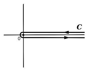
Figure 1: The contour of integration which result in eq.(4.29)

$$\tilde{Z}\Bigl{(}\frac{s}{\lambda(t)};t\Bigr{)}\;=\;\frac{\Gamma\bigl{(}1+s/\lambda(t)\bigr{)}}{2\pi i}\,\Biggl{[}\int_{+\infty}^{0}d\rho\,\rho^{s/\lambda(t)}\,\exp\bigl{\{}-G_{t}(\rho)\bigr{\}}\;+\;\int_{0}^{+\infty}d\rho\,\rho^{s/\lambda(t)}\exp\{2\pi is/\lambda(t)\}\,\exp\bigl{\{}-G_{t}(\rho)\bigr{\}}\Biggr{]}$$ (4.29)

Substituting $\rho\,=\,\exp\{\lambda(t)\,\xi\}$ and reorganizing the integration terms we gets

$$\tilde{Z}\Bigl{(}\frac{s}{\lambda(t)};t\Bigr{)}\;=\;-\Gamma\bigl{(}1+s/\lambda(t)\bigr{)}\;\frac{\lambda(t)}{2\pi i}\,\Bigl{[}1-\exp\bigl{\{}2\pi is/\lambda(t)\bigr{\}}\Bigr{]}\,\int_{-\infty}^{+\infty}\,d\xi\,\exp\bigl{\{}s\,\xi\,-\,G_{t}(\xi)\bigr{\}}$$ (4.30)

where the function $G_{t}(\xi)$ is defined in eqs.(4.26)-(4.27) with

$$S_{t}(z,y)\;\to\;S_{t}(\xi,y)\;=\;\frac{\kappa\,\exp\bigl{\{}\lambda(t)\,(y-\xi)\bigr{\}}}{1\;+\;\kappa\,\exp\bigl{\{}\lambda(t)\,(y-\xi)\bigr{\}}}$$ (4.31)

Performing the inverse Laplace transformation, eq.(2.11), for the free energy probability distribution function we get

$$P_{t}(f)\;=\;-\Gamma\bigl{(}1+s/\lambda(t)\bigr{)}\;\frac{\lambda(t)}{2\pi i}\,\int_{-\infty}^{+\infty}d\xi\int_{-i\infty}^{+i\infty}\frac{ds}{2\pi i}\,\Bigl{[}1-\exp\bigl{\{}2\pi is/\lambda(t)\bigr{\}}\Bigr{]}\,\exp\bigl{\{}s\,(\xi+f)\,-\,G_{t}(\xi)\bigr{\}}$$ (4.32)

Finally, taking the limit $t\to\infty$ (so that $\lambda(t)\to\infty$) we obtain

$$\lim_{t\to\infty}P_{t}(f)\,\equiv\,P_{GUE}(f) = \int_{-\infty}^{+\infty}d\xi\int_{-i\infty}^{+i\infty}\frac{ds}{2\pi i}\,s\,\exp\bigl{\{}s\,(\xi+f)\bigr{\}}\;\exp\bigl{\{}-\,G_{*}(\xi)\bigr{\}}$$ (4.33)

$$= \int_{-\infty}^{+\infty}d\xi\;\delta^{\prime}(\xi+f)\exp\bigl{\{}-\,G_{*}(\xi)\bigr{\}}\$$

$$= -\frac{\partial}{\partial f}\;\exp\bigl{\{}-\,G_{*}(-f)\bigr{\}}$$

where, according to eq.(4.26) and (4.27),

$$G_{*}(-f)\;=\;\sum_{M=1}^{\infty}\frac{1}{M}\;\mbox{Tr}\;\hat{K}_{A}^{M}$$ (4.34)

with

$$\mbox{Tr}\,\hat{K}_{A}^{M}\equiv\lim_{t\to\infty}\prod_{\alpha=1}^{M}\Biggl{[}\int_{0}^{\infty}d\omega_{\alpha}\int_{-\infty}^{\infty}dy\int_{-\infty}^{+\infty}\frac{dp}{2\pi}\operatorname{Ai}(y+p^{2}+\omega_{\alpha}+\omega_{\alpha-1})\;\exp\bigl{\{}ip(\omega_{\alpha}-\omega_{\alpha-1})\bigr{\}}\;S_{t}(z,y)\Biggr{]}$$ (4.35)

Using eq.(4.31) we find

$$\lim_{t\to\infty}S_{t}(-f,y)\;=\;\theta(y+f)$$ (4.36)

Thus, according eqs.(4.33)-(4.36) in the limit $t\to\infty$ the free energy probability density function is

$$P_{GUE}(f)\;=\;-\frac{\partial}{\partial f}\;\exp\Biggl{\{}-\sum_{M=1}^{\infty}\frac{1}{M}\;\mbox{Tr}\;\hat{K}_{A}^{M}\Biggr{\}}$$ (4.37)

where

$$\mbox{Tr}\;\hat{K}_{A}^{M}\;=\;\prod_{\alpha=1}^{M}\Biggl{[}\int_{0}^{\infty}d\omega_{\alpha}\int_{-\infty}^{\infty}dy\int_{-\infty}^{+\infty}\frac{dp}{2\pi}\operatorname{Ai}(y+p^{2}+\omega_{\alpha}+\omega_{\alpha-1})\;\exp\bigl{\{}ip(\omega_{\alpha}-\omega_{\alpha-1})\bigr{\}}\;\theta(y+f)\Biggr{]}$$ (4.38)

One can easily see that the above expression coincides with the one in (4.16) and (4.19) which defines the Fredholm determinant, eq.(4.21).

V GOE Tracy-Widom distribution in the model with free boundary conditions

In this Chapter we consider the system in which the polymer is fixed at the origin, $\phi(0)=0$ and it is free at $\tau=t$. In other words, for a given realization of the random potential $V$ the partition function of this system is:

$$Z(t)=\int_{-\infty}^{+\infty}dx\;Z(x;t)\;=\;\exp\{-\beta F(t)\}$$ (5.1)

where

$$Z(x;t)=\int_{\phi(0)=0}^{\phi(t)=x}{\cal D}\phi(\tau)\;\exp\bigl{\{}-\beta H[\phi;V]\bigr{\}}$$ (5.2)

is the partition function of the system with the fixed boundary conditions, $\phi(0)=0$ and $\phi(t)=x$. Here $F=f_{0}t\,+\,c\,t^{1/3}\,f$ is the total free energy (see discussion in Chapter I and eq.(1.8) and the Hamiltonian $H[\phi;V]$ is given in eq.(1.1). In this Chapter it will be shown that unlike the system with fixed boundary conditions (considered in Chapter IV) the probability distribution of the fluctuating part of the free energy $W(f)$, eq.(2.5), in the present system is the Gaussian orthogonal ensemble (GOE) Tracy-Widom distribution TW2 ; LeDoussal2 ; goe . Namely, in the limit limit, $t\to\infty$, this function is equal to the Fredholm determinant

$$W_{GOE}(f)\;=\;\det(1-\hat{K})\;\equiv\;F_{1}(-f)$$ (5.3)

where $\hat{K}$ is the integral operator on $[-f,\,+\infty)$ with the kernel Ferrari-Spohn

$$K(\omega,\omega^{\prime})\;=\;\operatorname{Ai}(\omega+\omega^{\prime}-f)\;;\;\;\;\;\;\;\;\;\;(\omega,\omega^{\prime}\;>0)$$ (5.4)

Explicitly TW2 ,

$$F_{1}(s)\;=\;\exp\Biggl{[}-\frac{1}{2}\int_{s}^{+\infty}d\xi\;(\xi-s)\;q^{2}(\xi)\;-\frac{1}{2}\int_{s}^{+\infty}d\xi\;q(\xi)\Biggr{]}$$ (5.5)

where $q(\xi)$ is the solution of the Panlevé II differential equation, $q^{\prime\prime}(\xi)=\xi q(\xi)+2q^{3}(\xi)$, with the boundary condition $q(\xi\to+\infty)=\operatorname{Ai}(\xi)$.

It should be noted that derivation given below is rather technical and the purpose of this Chapter is not only the final result (which is well known anyway) but the demonstration of the method and new technical tricks used in the derivation. The most cumbersome technical parts of the calculations are moved to the Appendix E.

Later on we will see that the integration over $x$ in the definition of the partition function, eq.(5.1), requires proper regularization at both limits $\pm\infty$. For that reason it is convenient to represent it in the form of two contributions:

$$Z(t)\;=\;\int_{-\infty}^{0}dx\;Z(x;t)\;+\;\int_{0}^{+\infty}dx\;Z(x;t)\;\equiv\;Z_{(-)}(t)\;+\;Z_{(+)}(t)$$ (5.6)

Correspondingly, following the same route as in Chapter III, for the replica partition function $\overline{Z^{N}(t)}=Z(N;t)$ instead of eq.(3.11) we get

$$Z(N;t)\;=\;\sum_{K,L=0}^{N}\frac{N!}{K!\,L!}\,\delta_{K+L,\,N}\int_{-\infty}^{0}dx_{1}...dx_{K}\int_{0}^{+\infty}dy_{1}...dy_{L}\Psi(x_{1},...,x_{K},y_{L},...,y_{1};t)$$ (5.7)

where

$$\Psi(x_{1},...,x_{K},y_{L},...,y_{1};t)\;=\;\overline{Z(x_{1};t)\,Z(x_{2};t)\,...\,Z(x_{K};t)\,Z(y_{L};t)\,Z(y_{L-1};t)\,...\,Z(y_{1};t)}$$ (5.8)

Explicitly, in terms of the Bethe ansatz solution the above wave function is given in eqs.(3.16) and (3.15). Next, repeating the calculations of Chapter III, instead of eq.(LABEL:4.1) we eventually get

$$\tilde{Z}(N;t) = N!\sum_{K,L=0}^{N}\,\delta_{K+L,\,N}\sum_{M=1}^{N}\,\frac{1}{M!}\prod_{\alpha=1}^{M}\Biggl{[}\sum_{n_{\alpha}=1}^{\infty}\int_{-\infty}^{+\infty}\frac{dq_{\alpha}\,\kappa^{n_{\alpha}}}{2\pi}\exp\Bigl{\{}-\frac{t}{2\beta}\,n_{\alpha}q_{\alpha}^{2}\,+\,\frac{\kappa^{2}\,t}{24\beta}n_{\alpha}^{3}\Bigr{\}}\Biggr{]}{\boldsymbol{\delta}}\Bigl{(}\sum_{\alpha=1}^{M}n_{\alpha}\;,\;N\Bigr{)}\times$$

$$\times \det\Biggl{[}\frac{1}{\frac{1}{2}\kappa n_{\alpha}-iq_{\alpha}+\frac{1}{2}\kappa n_{\beta}+iq_{\beta}}\Biggr{]}_{\alpha,\beta=1,...M}I_{K,L}({\bf q},{\bf n})$$

where

$$I_{K,L}({\bf q},{\bf n}) = \frac{1}{K!\,L!}\sum_{{\cal P}\in S_{N}}\;\int_{-\infty}^{0}dx_{1}...dx_{K}\int_{0}^{+\infty}dy_{1}...dy_{L}\;\exp\Biggl{[}i\sum_{a=1}^{K}\Bigl{(}Q_{{\cal P}_{a}}-i\epsilon\Bigr{)}x_{a}\;+\;i\sum_{c=1}^{L}\Bigl{(}Q_{{\cal P}_{c}}-i\epsilon\Bigr{)}y_{c}\Biggr{]}\times\$$ (5.10)

$$\times \prod_{a<b}^{K}\Biggl{[}1+i\kappa\frac{\operatorname{sgn}(x_{a}-x_{b})}{Q_{{\cal P}_{a}}-Q_{{\cal P}_{b}}}\Biggr{]}\;\prod_{c<d}^{L}\Biggl{[}1+i\kappa\frac{\operatorname{sgn}(y_{c}-y_{d})}{Q_{{\cal P}_{c}}-Q_{{\cal P}_{d}}}\Biggr{]}\;\prod_{a=1}^{K}\prod_{c=1}^{L}\Biggl{[}1+i\kappa\frac{\operatorname{sgn}(x_{a}-y_{c})}{Q_{{\cal P}_{a}}-Q_{{\cal P}_{c}}}\Biggr{]}$$

Here the summation goes over all permutations $P$ of $N$ momenta $\{Q_{1},...,Q_{N}\}$ over $K+L=N$ particles $\{x_{1},...,x_{K},y_{L},...,y_{1}\}$. Note also that the integrations both over $x_{a}$’s and over $y_{c}$’s in eq.(5.10) require proper regularization at $-\infty$ and $+\infty$ correspondingly. This is done in the standard way by introducing a supplementary parameter $\epsilon$ which will be set to zero in final results. Due to the symmetry of the above expression with respect to permutations among $x_{a}$’s and $y_{c}$’s it can be represented as follows

$$I_{K,L}({\bf q},{\bf n}) = \sum_{{\cal P}^{(K,L)}}\sum_{{\cal P}^{(K)}}\sum_{{\cal P}^{(L)}}\;\prod_{a=1}^{K}\prod_{c=1}^{L}\Biggl{[}\frac{Q_{{\cal P}_{a}^{(K)}}-Q_{{\cal P}_{c}^{(L)}}-i\kappa}{Q_{{\cal P}_{a}^{(K)}}-Q_{{\cal P}_{c}^{(L)}}}\Biggr{]}\times\prod_{a<b}^{K}\Biggl{[}\frac{Q_{{\cal P}_{a}^{(K)}}-Q_{{\cal P}_{b}^{(K)}}-i\kappa}{Q_{{\cal P}_{a}^{(K)}}-Q_{{\cal P}_{b}^{(K)}}}\Biggr{]}\times\prod_{c<d}^{L}\Biggl{[}\frac{Q_{{\cal P}_{c}^{(L)}}-Q_{{\cal P}_{d}^{(L)}}+i\kappa}{Q_{{\cal P}_{c}^{(L)}}-Q_{{\cal P}_{d}^{(L)}}}\Biggr{]}\times$$ (5.11)

$$\times \int_{-\infty<x_{1}\leq...\leq x_{K}\leq 0}dx_{1}...dx_{K}\;\exp\Bigl{[}i\sum_{a=1}^{K}(Q_{{\cal P}_{a}^{(K)}}-i\epsilon)x_{a}\Bigr{]}$$

$$\times \int_{0\leq y_{L}\leq...\leq y_{1}<+\infty}dy_{L}...dy_{1}\;\exp\Bigl{[}i\sum_{c=1}^{L}(Q_{{\cal P}_{c}^{(L)}}+i\epsilon)y_{c}\Bigr{]}$$

Here the summation over all permutations ${\cal P}$ is split into three parts: the permutations ${\cal P}^{(K)}$ of $K$ momenta (taken at random out of the total list $\{Q_{1},...,Q_{K+L}\}$) over $K$ ”negative” particles $\{x_{1},...,x_{K}\}$, the permutations ${\cal P}^{(L)}$ of the remaining $L$ momenta over $L$ ”positive” particles $\{y_{L},...,y_{1}\}$, and finally the permutations ${\cal P}^{(K,L)}$ (or the exchange) of the momenta between the group $"K"$ and the group $"L"$.

Performing the integrations in eq.(5.11) we get:

$$I_{K,L}({\bf q},{\bf n}) = i^{-(K+L)}\sum_{{\cal P}^{(K,L)}}\;\;\prod_{a=1}^{K}\prod_{c=1}^{L}\Biggl{[}\frac{Q_{{\cal P}_{a}^{(K)}}-Q_{{\cal P}_{c}^{(L)}}-i\kappa}{Q_{{\cal P}_{a}^{(K)}}-Q_{{\cal P}_{c}^{(L)}}}\Biggr{]}\times$$ (5.12)

$$\times \sum_{{\cal P}^{(K)}}\;\;\frac{1}{Q^{(-)}_{{\cal P}_{1}^{(K)}}\bigl{(}Q^{(-)}_{{\cal P}_{1}^{(K)}}+Q^{(-)}_{{\cal P}_{2}^{(K)}}\bigr{)}...\bigl{(}Q^{(-)}_{{\cal P}_{1}^{(K)}}+...+Q^{(-)}_{{\cal P}_{K}^{(K)}}\bigr{)}}\prod_{a<b}^{K}\Biggl{[}\frac{Q^{(-)}_{{\cal P}_{a}^{(K)}}-Q^{(-)}_{{\cal P}_{b}^{(K)}}-i\kappa}{Q^{(-)}_{{\cal P}_{a}^{(K)}}-Q^{(-)}_{{\cal P}_{b}^{(K)}}}\Biggr{]}\times$$

$$\times \sum_{{\cal P}^{(L)}}\;\;\frac{(-1)^{L}}{Q^{(+)}_{{\cal P}_{1}^{(L)}}\bigl{(}Q^{(+)}_{{\cal P}_{1}^{(L)}}+Q^{(+)}_{{\cal P}_{2}^{(L)}}\bigr{)}...\bigl{(}Q^{(+)}_{{\cal P}_{1}^{(L)}}+...+Q^{(+)}_{{\cal P}_{L}^{(L)}}\bigr{)}}\prod_{c<d}^{L}\Biggl{[}\frac{Q^{(+)}_{{\cal P}_{c}^{(L)}}-Q^{(+)}_{{\cal P}_{d}^{(L)}}+i\kappa}{Q^{(+)}_{{\cal P}_{c}^{(L)}}-Q^{(+)}_{{\cal P}_{d}^{(L)}}}\Biggr{]}$$

where

$$Q^{(\pm)}_{a}\;\equiv\;Q_{a}\pm i\epsilon$$ (5.13)

Using the Bethe ansatz combinatorial identity LeDoussal2 (Appendix D),

$$\sum_{P\in S_{N}}\frac{1}{Q_{P_{1}}(Q_{P_{1}}+Q_{P_{2}})...(Q_{P_{1}}+...+Q_{P_{N}})}\prod_{a<b}^{N}\Biggl{[}\frac{Q_{P_{a}}-Q_{P_{b}}-i\kappa}{Q_{P_{a}}-Q_{P_{b}}}\Biggr{]}\;=\;\frac{1}{\prod_{a=1}^{N}Q_{a}}\;\prod_{a<b}^{N}\Biggl{[}\frac{Q_{a}+Q_{b}+i\kappa}{Q_{a}+Q_{b}}\Biggr{]}$$ (5.14)

(where the summation goes over all permutations of $N$ momenta $\{Q_{1},...,Q_{N}\}$) we get:

$$I_{K,L}({\bf q},{\bf n}) = i^{-(K+L)}\sum_{{\cal P}^{(K,L)}}\;\;\prod_{a=1}^{K}\prod_{c=1}^{L}\Biggl{[}\frac{Q_{{\cal P}_{a}^{(K)}}-Q_{{\cal P}_{c}^{(L)}}-i\kappa}{Q_{{\cal P}_{a}^{(K)}}-Q_{{\cal P}_{c}^{(L)}}}\Biggr{]}\times$$ (5.15)

$$\times \frac{1}{\prod_{a=1}^{K}Q^{(-)}_{{\cal P}_{a}^{(K)}}}\prod_{a<b}^{K}\Biggl{[}\frac{Q^{(-)}_{{\cal P}_{a}^{(K)}}+Q^{(-)}_{{\cal P}_{b}^{(K)}}+i\kappa}{Q^{(-)}_{{\cal P}_{a}^{(K)}}+Q^{(-)}_{{\cal P}_{b}^{(K)}}}\Biggr{]}\times\frac{(-1)^{L}}{\prod_{c=1}^{L}Q^{(+)}_{{\cal P}_{c}^{(L)}}}\prod_{c<d}^{L}\Biggl{[}\frac{Q^{(+)}_{{\cal P}_{c}^{(L)}}+Q^{(+)}_{{\cal P}_{d}^{(L)}}-i\kappa}{Q^{(+)}_{{\cal P}_{c}^{(L)}}+Q^{(+)}_{{\cal P}_{d}^{(L)}}}\Biggr{]}$$

Substituting now eq.(LABEL:5.9) with $I_{K,L}({\bf q},{\bf n})$ given in eq.(5.15) into the expression for the probability distribution function, eq.(2.19), and taking into account that $N\;=\;K+L$ we obtain

$$W(f) = \lim_{t\to\infty}\sum_{K,L=0}^{\infty}(-1)^{K+L}\sum_{M=0}^{\infty}\frac{(-1)^{M}}{M!}\prod_{\alpha=1}^{M}\Biggl{[}\sum_{n_{\alpha}=1}^{\infty}\,(-1)^{n_{\alpha}-1}\int_{-\infty}^{+\infty}\frac{dq_{\alpha}\,\kappa^{n_{\alpha}}}{2\pi}\exp\Bigl{\{}\lambda(t)n_{\alpha}\,f-\frac{t}{2\beta}\,n_{\alpha}q_{\alpha}^{2}\,+\,\frac{\kappa^{2}\,t}{24\beta}n_{\alpha}^{3}\Bigr{\}}\Biggr{]}\times$$

$$\times \det\Biggl{[}\frac{1}{\frac{1}{2}\kappa n_{\alpha}-iq_{\alpha}+\frac{1}{2}\kappa n_{\beta}+iq_{\beta}}\Biggr{]}_{\alpha,\beta=1,...M}I_{K,L}({\bf q},{\bf n})\;\,{\boldsymbol{\delta}}\Bigl{(}\sum_{\alpha=1}^{M}n_{\alpha}\;,\;K+L\Bigr{)}$$

Further simplification comes due to the special Bethe ansatz product structure of the factor $I_{K,L}({\bf q},{\bf n})$, eq.(5.15). One can easily see that in these products, according to the definition (3.13), the momenta $Q_{a}$ belonging to the same cluster must be ordered. In other words, if we consider the momenta, eq.(3.13), of a cluster $\alpha$, $\{q_{1}^{\alpha},q_{2}^{\alpha},...,q_{n_{\alpha}}^{\alpha}\}$, the permutation of any two momenta $q_{r}^{\alpha}$ and $q_{r^{\prime}}^{\alpha}$ of this ordered set gives zero contribution to the factor $I_{K,L}({\bf q},{\bf n})$. Thus, in order to perform the summation over the permutations ${\cal P}^{(K,L)}$ in eq.(5.15) it is sufficient to split the momenta of each cluster into two parts: $\{q_{1}^{\alpha},...,q_{m_{\alpha}}^{\alpha}||q_{m_{\alpha}+1}^{\alpha}...,q_{n_{\alpha}}^{\alpha}\}$, where $m_{\alpha}=0,1,...,n_{\alpha}$ and the momenta $q_{1}^{\alpha},...,q_{m_{\alpha}}^{\alpha}$ belong to the sector $"K"$, while the momenta $q_{m_{\alpha}+1}^{\alpha}...,q_{n_{\alpha}}^{\alpha}$ belong to the sector $"L"$.

It is convenient to introduce the numbering of the momenta of the sector $"L"$ in the reversed order:

$$q_{n_{\alpha}}^{\alpha} \to {q^{*}}_{1}^{\alpha}$$

$$q_{n_{\alpha}-1}^{\alpha} \to {q^{*}}_{2}^{\alpha}$$

$$........$$

$$q_{m_{\alpha}+1}^{\alpha} \to {q^{*}}_{s_{\alpha}}^{\alpha}$$ (5.17)

where $m_{\alpha}+s_{\alpha}=n_{\alpha}$ and (s.f. eq.(3.13))

$${q^{*}}_{r}^{\alpha}\;=\;q_{\alpha}+\frac{i\kappa}{2}(n_{\alpha}+1-2r)\;=\;q_{\alpha}+\frac{i\kappa}{2}(m_{\alpha}+s_{\alpha}+1-2r)$$ (5.18)

By definition, the integer parameters $\{m_{\alpha}\}$ and $\{s_{\alpha}\}$ fulfill the global constrains

$$\sum_{\alpha=1}^{M}m_{\alpha} = K$$ (5.19)

$$\sum_{\alpha=1}^{M}s_{\alpha} = L$$ (5.20)

In this way the summation over permutations ${\cal P}^{(K,L)}$ in eq.(5.15) is changed by the summations over the integer parameters $\{m_{\alpha}\}$ and $\{s_{\alpha}\}$:

$$\sum_{{\cal P}^{(K,L)}}\;\bigl{(}...\bigr{)}\;\to\;\prod_{\alpha=1}^{M}\Biggl{[}\sum_{m_{\alpha}+s_{\alpha}\geq 1}^{\infty}\;{\boldsymbol{\delta}}\Bigl{(}m_{\alpha}+s_{\alpha}\;,\;n_{\alpha}\Bigr{)}\Biggr{]}\;{\boldsymbol{\delta}}\Bigl{(}\sum_{\alpha=1}^{M}m_{\alpha}\;,\;K\Bigr{)}\;{\boldsymbol{\delta}}\Bigl{(}\sum_{\alpha=1}^{M}s_{\alpha}\;,\;L\Bigr{)}\;\bigl{(}...\bigr{)}$$ (5.21)

which allows to lift the summations over $K$, $L$, and $\{n_{\alpha}\}$ in eq.(LABEL:5.16):

$$W(f) = \lim_{t\to\infty}\sum_{M=0}^{\infty}\frac{(-1)^{M}}{M!}\prod_{\alpha=1}^{M}\Biggl{[}\sum_{m_{\alpha}+s_{\alpha}\geq 1}^{\infty}\,(-1)^{m_{\alpha}+s_{\alpha}-1}\,\kappa^{m_{\alpha}+s_{\alpha}}\int_{-\infty}^{+\infty}\frac{dq_{\alpha}}{2\pi}$$

$$\times \exp\Bigl{\{}\lambda(t)(m_{\alpha}+s_{\alpha})\,f-\frac{t}{2\beta}\,(m_{\alpha}+s_{\alpha})q_{\alpha}^{2}\,+\,\frac{\kappa^{2}\,t}{24\beta}(m_{\alpha}+s_{\alpha})^{3}\Bigr{\}}\Biggr{]}$$

$$\times \det\Biggl{[}\frac{1}{\frac{1}{2}\kappa(m_{\alpha}+s_{\alpha})-iq_{\alpha}+\frac{1}{2}\kappa(m_{\beta}+s_{\beta})+iq_{\beta}}\Biggr{]}_{\alpha,\beta=1,...M}I_{K,L}({\bf q};{\bf m},{\bf s})$$

Next, after somewhat painful algebra the factor $I_{K,L}({\bf q};{\bf m},{\bf s})$, eq.(5.15), can be represented in terms of the product of the Gamma functions (see Appendix E). Then, redefining the momenta, $q_{\alpha}=\kappa\,p_{\alpha}/(2\lambda)$ and performing the same transformations as in eqs.(4.5)-(4.7) we get (s.f. eq.(LABEL:4.8))

$$W(f) = \lim_{t\to\infty}\sum_{M=1}^{\infty}\;\frac{(-1)^{M}}{M!}\;\prod_{\alpha=1}^{M}\Biggl{[}\int\int_{-\infty}^{+\infty}\frac{dy_{\alpha}dp_{\alpha}}{2\pi}\operatorname{Ai}\bigl{(}y_{\alpha}+p_{\alpha}^{2}-f\bigr{)}$$ (5.23)

$$\times \sum_{m_{\alpha}+s_{\alpha}\geq 1}^{\infty}(-1)^{m_{\alpha}+s_{\alpha}-1}\exp\bigl{\{}\lambda(t)(m_{\alpha}+s_{\alpha})y_{\alpha}\bigr{\}}\;{\cal G}\Bigl{(}\frac{p_{\alpha}}{\lambda(t)},\;m_{\alpha},\;s_{\alpha}\Bigr{)}\;\Biggr{]}$$

$$\times \det\Biggl{[}\frac{1}{\lambda(t)(m_{\alpha}+s_{\alpha})-ip_{\alpha}+\lambda(t)(m_{\beta}+s_{\beta})+ip_{\beta}}\Biggr{]}_{\alpha,\beta=1,...M}\times\prod_{1\leq\alpha<\beta}^{M}\;{\cal G}_{\alpha\beta}\Bigl{(}\frac{{\bf p}}{\lambda(t)},\;{\bf m},\;{\bf s}\Bigr{)}$$

where (see eq.(E.17)

$${\cal G}\bigl{(}\frac{p_{\alpha}}{\lambda},m_{\alpha},s_{\alpha}\bigr{)}\;=\;\frac{\Gamma\Bigl{(}s_{\alpha}+i{p_{\alpha}}^{(-)}/\lambda\Bigr{)}\,\Gamma\Bigl{(}m_{\alpha}-i{p_{\alpha}}^{(+)}/\lambda\Bigr{)}\,\Gamma\bigl{(}1+m_{\alpha}+s_{\alpha}\bigr{)}}{2^{(m_{\alpha}+s_{\alpha})}\Gamma\Bigl{(}m_{\alpha}+s_{\alpha}+i{p_{\alpha}}^{(-)}/\lambda\Bigr{)}\,\Gamma\Bigl{(}m_{\alpha}+s_{\alpha}-i{p_{\alpha}}^{(+)}/\lambda\Bigr{)}\,\Gamma\bigl{(}1+m_{\alpha}\bigr{)}\Gamma\bigl{(}1+s_{\alpha}\bigr{)}}$$ (5.24)

and the explicit expression for the factor ${\cal G}_{\alpha\beta}\bigl{(}{\bf q},\;{\bf m},\;{\bf s}\bigr{)}$ is given in eq.(E.18).

The crucial point of the further calculations is taking the limit $t\to\infty$. Reorganizing the terms, the expression in eq.(5.23) can be represented as follows

$$W(f)\;=\;\sum_{M=0}^{\infty}\;\frac{(-1)^{M}}{M!}\;\prod_{\alpha=1}^{M}\Biggl{[}\int\int_{-\infty}^{+\infty}\frac{dy_{\alpha}dp_{\alpha}}{2\pi}\operatorname{Ai}\bigl{(}y_{\alpha}+p_{\alpha}^{2}-f\bigr{)}\Biggr{]}\;{\cal S}_{M}\bigl{(}{\bf p},{\bf y}\bigr{)}$$ (5.25)

where

$${\cal S}_{M}\bigl{(}{\bf p},{\bf y}\bigr{)} = \lim_{t\to\infty}\prod_{\alpha=1}^{M}\Biggl{[}\sum_{m_{\alpha}+s_{\alpha}\geq 1}^{\infty}(-1)^{m_{\alpha}+s_{\alpha}-1}\exp\bigl{\{}\lambda(t)m_{\alpha}y_{\alpha}+\lambda(t)s_{\alpha}y_{\alpha}\bigr{\}}\Biggr{]}\times\prod_{\alpha=1}^{M}\Biggl{[}{\cal G}\Bigl{(}\frac{p_{\alpha}}{\lambda(t)},\;m_{\alpha},\;s_{\alpha}\Bigr{)}\;\Biggr{]}\times$$ (5.26)

$$\times \prod_{1\leq\alpha<\beta}^{M}\Biggl{[}{\cal G}_{\alpha\beta}\Bigl{(}\frac{{\bf p}}{\lambda(t)},\;{\bf m},\;{\bf s}\Bigr{)}\Biggr{]}\;\det\Biggl{[}\frac{1}{\lambda(t)(m_{\alpha}+s_{\alpha})-ip_{\alpha}+\lambda(t)(m_{\beta}+s_{\beta})+ip_{\beta}}\Biggr{]}_{\alpha,\beta=1,...M}$$

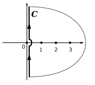
Figure 2: The contour of integration in eq.(5.28)

In the limit $t\to\infty$ the summations over $\{m_{\alpha}\}$ and $\{s_{\alpha}\}$ in the above expression can performed according to the following algorithm. Let us consider the sum of a general type:

$$R({\bf y},{\bf p})\;=\;\lim_{\lambda\to\infty}\prod_{\alpha=1}^{M}\Biggl{[}\sum_{n_{\alpha}=1}^{\infty}\;(-1)^{n_{\alpha}-1}\exp\{\lambda n_{\alpha}y_{\alpha}\}\Biggr{]}\;\Phi\Bigl{(}{\bf p},\;\frac{{\bf p}}{\lambda},\;\lambda{\bf n},\;{\bf n}\Bigr{)}$$ (5.27)

where $\Phi$ is a ”good” function which depend on the factors $p_{\alpha}$, $p_{\alpha}/\lambda$, $\lambda n_{\alpha}$ and $n_{\alpha}$. One can easily see that the summations in eq.(5.27) can be changed by of the integrations in the complex plane:

$$R({\bf y},{\bf p})\;=\;\lim_{\lambda\to\infty}\prod_{\alpha=1}^{M}\Biggl{[}\frac{1}{2i}\int_{{\cal C}}\frac{dz_{\alpha}}{\sin(\pi z_{\alpha})}\exp\{\lambda z_{\alpha}y_{\alpha}\}\Biggr{]}\;\Phi\Bigl{(}{\bf p},\;\frac{{\bf p}}{\lambda},\;\lambda{\bf z},\;{\bf z}\Bigr{)}$$ (5.28)

where the integration goes over the contour ${\cal C}$ shown in Fig.2, and it is assumed that the function $\Phi$ is such that there is no contribution from $\infty$. Indeed, due to the sign alternating contributions of simple poles at integer $z=1,2,...$, eq.(5.28) reduces to eq.(5.27). Then, redefining $z\to z/\lambda$, in the limit $\lambda\to\infty$ we get:

$$R({\bf y},{\bf p}) = \prod_{\alpha=1}^{M}\Biggl{[}\frac{1}{2\pi i}\int_{{\cal C}}\frac{dz_{\alpha}}{z_{\alpha}}\exp\{z_{\alpha}y_{\alpha}\}\Biggr{]}\;\lim_{\lambda\to\infty}\Phi\Bigl{(}{\bf p},\;\frac{{\bf p}}{\lambda},\;{\bf z},\;\frac{{\bf z}}{\lambda}\Bigr{)}$$ (5.29)

$$= \prod_{\alpha=1}^{M}\Biggl{[}\frac{1}{2\pi i}\int_{{\cal C}}\frac{dz_{\alpha}}{z_{\alpha}}\exp\{z_{\alpha}y_{\alpha}\}\Biggr{]}\;\Phi\Bigl{(}{\bf p},\;{\bf 0},\;{\bf z},\;{\bf 0}\Bigr{)}$$

Coming back to eq.(5.26), the summations over $m_{\alpha}$ and $s_{\alpha}$ can be represented as follows

$$\sum_{m_{\alpha}+s_{\alpha}\geq 1}^{\infty}(-1)^{m_{\alpha}+s_{\alpha}-1}=\sum_{m_{\alpha}=1}^{\infty}(-1)^{m_{\alpha}-1}\delta(s_{\alpha},0)+\sum_{s_{\alpha}=1}^{\infty}(-1)^{s_{\alpha}-1}\delta(m_{\alpha},0)-\sum_{m_{\alpha}=1}^{\infty}(-1)^{m_{\alpha}-1}\sum_{s_{\alpha}=1}^{\infty}(-1)^{s_{\alpha}-1}$$ (5.30)

Thus in the integral representation, following the algorithm eqs.(5.27)-(5.29), we get

$${\cal S}_{M}\bigl{(}{\bf p},{\bf y}\bigr{)} = \prod_{\alpha=1}^{M}\Biggl{[}\int\int_{{\cal C}}\frac{d{z_{1}}_{\alpha}d{z_{2}}_{\alpha}}{(2\pi i)^{2}}\Bigl{(}\frac{2\pi i}{{z_{1}}_{\alpha}}\delta({z_{2}}_{\alpha})+\frac{2\pi i}{{z_{2}}_{\alpha}}\delta({z_{1}}_{\alpha})-\frac{1}{{z_{1}}_{\alpha}{z_{2}}_{\alpha}}\Bigr{)}\exp\bigl{\{}{z_{1}}_{\alpha}y_{\alpha}+{z_{2}}_{\alpha}y_{\alpha}\bigr{\}}\Biggr{]}\times$$ (5.31)

$$\times \det\Bigl{[}\frac{1}{{z_{1}}_{\alpha}+{z_{2}}_{\alpha}-ip_{\alpha}+{z_{1}}_{\beta}+{z_{2}}_{\beta}+ip_{\beta}}\Bigr{]}_{(\alpha,\beta)=1,2,...,M}\times$$

$$\times \lim_{t\to\infty}\Biggl{\{}\prod_{\alpha=1}^{M}\Biggl{[}{\cal G}\Bigl{(}\frac{p_{\alpha}}{\lambda(t)},\;\frac{{z_{1}}_{\alpha}}{\lambda(t)},\;\frac{{z_{2}}_{\alpha}}{\lambda(t)}\Bigr{)}\;\Biggr{]}\;\prod_{1\leq\alpha<\beta}^{M}\Biggl{[}{\cal G}_{\alpha\beta}\Bigl{(}\frac{{\bf p}}{\lambda(t)},\;\frac{{\bf z_{1}}}{\lambda(t)},\;\frac{{\bf z_{2}}}{\lambda(t)}\Bigr{)}\Biggr{]}\Biggr{\}}$$

Taking into account the Gamma function properties, $\Gamma(z)|_{|z|\to 0}=1/z$ and $\Gamma(1+z)|_{|z|\to 0}=1$, for the factors ${\cal G}$, eq.(5.24), and ${\cal G}_{\alpha\beta}$, eq.(E.18), we obtain

$$\lim_{t\to\infty}{\cal G}\Bigl{(}\frac{p_{\alpha}}{\lambda(t)},\;\frac{{z_{1}}_{\alpha}}{\lambda(t)},\;\frac{{z_{2}}_{\alpha}}{\lambda(t)}\Bigr{)}\;=\;\frac{\bigl{(}{z_{1}}_{\alpha}+{z_{2}}_{\alpha}+ip_{\alpha}^{(-)}\bigr{)}\bigl{(}{z_{1}}_{\alpha}+{z_{2}}_{\alpha}-ip_{\alpha}^{(+)}\bigr{)}}{\bigl{(}{z_{2}}_{\alpha}+ip_{\alpha}^{(-)}\bigr{)}\bigl{(}{z_{1}}_{\alpha}-ip_{\alpha}^{(+)}\bigr{)}}$$ (5.32)

and

$$\lim_{t\to\infty}{\bf G}\Bigl{(}\frac{{\bf p}}{\lambda(t)},\;\frac{{\bf z}_{1}}{\lambda(t)},\;\frac{{\bf z}_{2}}{\lambda(t)}\Bigr{)}\;=\;1$$ (5.33)

Substituting eqs.(5.32) and (5.33) into eq.(5.31) and then eq.(5.31) into eq.(5.25) we see that in the limit $t\to\infty$ the expression for the probability distribution function, eq.(5.25), takes the form of the Fredholm determinant

$$W(f) = \sum_{M=0}^{\infty}\;\frac{(-1)^{M}}{M!}\;\prod_{\alpha=1}^{M}\Biggl{[}\int\int_{-\infty}^{+\infty}\frac{dy_{\alpha}dp_{\alpha}}{2\pi}\operatorname{Ai}\bigl{(}y_{\alpha}+p_{\alpha}^{2}-f\bigr{)}$$ (5.34)

$$\times \int\int_{{\cal C}}\frac{d{z_{1}}_{\alpha}d{z_{2}}_{\alpha}}{(2\pi i)^{2}}\Bigl{(}\frac{2\pi i}{{z_{1}}_{\alpha}}\delta({z_{2}}_{\alpha})+\frac{2\pi i}{{z_{2}}_{\alpha}}\delta({z_{1}}_{\alpha})-\frac{1}{{z_{1}}_{\alpha}{z_{2}}_{\alpha}}\Bigr{)}\Bigl{(}1+\frac{{z_{1}}_{\alpha}}{{z_{2}}_{\alpha}+ip_{\alpha}^{(-)}}\Bigr{)}\Bigl{(}1+\frac{{z_{2}}_{\alpha}}{{z_{1}}_{\alpha}-ip_{\alpha}^{(+)}}\Bigr{)}\times$$

$$\times \exp\bigl{\{}{z_{1}}_{\alpha}y_{\alpha}+{z_{2}}_{\alpha}y_{\alpha}\bigr{\}}\Biggr{]}\det\Bigl{[}\frac{1}{{z_{1}}_{\alpha}+{z_{2}}_{\alpha}-ip_{\alpha}+{z_{1}}_{\beta}+{z_{2}}_{\beta}+ip_{\beta}}\Bigr{]}_{(\alpha,\beta)=1,2,...,M}$$

$$= \det\bigl{[}1\,-\,\hat{K}\bigr{]}$$

with the kernel

$$\hat{K}\bigl{[}({z_{1}},\,{z_{2}},\,p);({z_{1}}^{\prime},\,{z_{2}}^{\prime},\,p^{\prime})\bigr{]} = \int_{-\infty}^{+\infty}\frac{dy}{2\pi}\operatorname{Ai}\bigl{(}y+p^{2}-f\bigr{)}\Bigl{(}\frac{2\pi i}{z_{1}}\delta(z_{2})+\frac{2\pi i}{z_{2}}\delta(z_{1})-\frac{1}{z_{1}{z_{2}}}\Bigr{)}\times$$ (5.35)

$$\times \Bigl{(}1+\frac{z_{1}}{z_{2}+ip^{(-)}}\Bigr{)}\Bigl{(}1+\frac{z_{2}}{z_{1}-ip^{(+)}}\Bigr{)}\frac{\exp\bigl{\{}z_{1}y+z_{2}y\bigr{\}}}{{z_{1}}+{z_{2}}-ip+{z_{1}}^{\prime}+{z_{2}}^{\prime}+ip^{\prime}}$$

In the exponential representation of this determinant we get

$$W(f)\;=\;\exp\Bigl{[}-\sum_{M=1}^{\infty}\frac{1}{M}\;\mbox{Tr}\,\hat{K}^{M}\Bigr{]}$$ (5.36)

where

$$\mbox{Tr}\,\hat{K}^{M} = \prod_{\alpha=1}^{M}\Biggl{[}\int\int_{-\infty}^{+\infty}\frac{dy_{\alpha}dp_{\alpha}}{2\pi}\operatorname{Ai}\bigl{(}y_{\alpha}+p_{\alpha}^{2}-f\bigr{)}\times$$ (5.37)

$$\times \int\int_{{\cal C}}\frac{d{z_{1}}_{\alpha}d{z_{2}}_{\alpha}}{(2\pi i)^{2}}\Bigl{(}\frac{2\pi i}{{z_{1}}_{\alpha}}\delta({z_{2}}_{\alpha})+\frac{2\pi i}{{z_{2}}_{\alpha}}\delta({z_{1}}_{\alpha})-\frac{1}{{z_{1}}_{\alpha}{z_{2}}_{\alpha}}\Bigr{)}\Bigl{(}1+\frac{{z_{1}}_{\alpha}}{{z_{2}}_{\alpha}+ip_{\alpha}^{(-)}}\Bigr{)}\Bigl{(}1+\frac{{z_{2}}_{\alpha}}{{z_{1}}_{\alpha}-ip_{\alpha}^{(+)}}\Bigr{)}\times$$

$$\times \exp\bigl{\{}{z_{1}}_{\alpha}y_{\alpha}+{z_{2}}_{\alpha}y_{\alpha}\bigr{\}}\Biggr{]}\;\prod_{\alpha=1}^{M}\Biggl{[}\frac{1}{{z_{1}}_{\alpha}+{z_{2}}_{\alpha}-ip_{\alpha}+{z_{1}}_{\alpha+1}+{z_{2}}_{\alpha+1}+ip_{\alpha+1}}\Biggr{]}$$

Here, by definition, it is assumed that ${z_{i_{M+1}}}\equiv{z_{i_{1}}}$ ($i=1,2$) and $p_{M+1}\equiv p_{1}$. Substituting

$$\frac{1}{{z_{1}}_{\alpha}+{z_{2}}_{\alpha}-ip_{\alpha}+{z_{1}}_{\alpha+1}+{z_{2}}_{\alpha+1}+ip_{\alpha+1}}\;=\;\int_{0}^{\infty}d\omega_{\alpha}\exp\Bigl{[}-\bigl{(}{z_{1}}_{\alpha}+{z_{2}}_{\alpha}-ip_{\alpha}+{z_{1}}_{\alpha+1}+{z_{2}}_{\alpha+1}+ip_{\alpha+1}\bigr{)}\,\omega_{\alpha}\Bigr{]}$$ (5.38)

into eq.(5.37), we obtain

$$\mbox{Tr}\,\hat{K}^{M}\;=\;\int_{0}^{\infty}d\omega_{1}\,...\,d\omega_{M}\,\prod_{\alpha=1}^{M}\Biggl{[}\int\int_{-\infty}^{+\infty}\frac{dydp}{2\pi}\operatorname{Ai}\bigl{(}y+p^{2}+\omega_{\alpha}+\omega_{\alpha-1}-f\bigr{)}\exp\{ip\bigl{(}\omega_{\alpha}-\omega_{\alpha-1}\bigr{)}\}\;S\bigl{(}p,y\bigr{)}\Biggr{]}$$ (5.39)

where, by definition, $\omega_{0}\equiv\omega_{M}$, and

$$S(p,y) = \int\int_{{\cal C}}\frac{dz_{1}dz_{2}}{(2\pi i)^{2}}\Bigl{(}\frac{2\pi i}{z_{1}}\delta(z_{2})+\frac{2\pi i}{z_{2}}\delta(z_{1})-\frac{1}{z_{1}z_{2}}\Bigr{)}\Bigl{(}1+\frac{z_{1}}{z_{2}+ip^{(-)}}\Bigr{)}\Bigl{(}1+\frac{z_{2}}{z_{1}-ip^{(+)}}\Bigr{)}\times$$ (5.40)

$$\times \exp\bigl{\{}z_{1}y+z_{2}y\bigr{\}}$$

Simple calculations yield:

$$S\bigl{(}p,\,y\bigr{)} = \frac{1}{2\pi i}\int_{{\cal C}}\frac{dz_{1}}{z_{1}}\,\Bigl{(}1+\frac{z_{1}}{i(p-i\epsilon)}\Bigr{)}\,\exp\{z_{1}y\}\;+\;\frac{1}{2\pi i}\int_{{\cal C}}\frac{dz_{2}}{z_{2}}\,\Bigl{(}1-\frac{z_{2}}{i(p+i\epsilon)}\Bigr{)}\,\exp\{z_{2}y\}\;-$$ (5.41)

$$- \frac{1}{(2\pi i)^{2}}\int\int_{{\cal C}}\frac{dz_{1}}{z_{1}}\,\frac{dz_{2}}{z_{2}}\Bigl{(}1+\frac{z_{1}}{z_{2}+i(p-i\epsilon)}\Bigr{)}\Bigl{(}1+\frac{z_{2}}{z_{1}-i(p+i\epsilon)}\Bigr{)}\exp\{(z_{1}+z_{2})y\}$$

$$= \Bigl{[}\frac{1}{i(p-i\epsilon)}-\frac{1}{i(p+i\epsilon)}\Bigr{]}\;\delta(y)$$

Taking the limit $\epsilon\to 0$ we find:

$$S\bigl{(}p,\,y\bigr{)}\;=\;\delta(y)\delta(p)$$ (5.42)

Substituting this result into eq.(5.39) we obtain

$$\mbox{Tr}\,\hat{K}^{M}\;=\;\int_{0}^{\infty}d\omega_{1}\,...\,d\omega_{M}\,\prod_{\alpha=1}^{M}\Bigl{[}\operatorname{Ai}\bigl{(}\omega_{\alpha}+\omega_{\alpha-1}-f\bigr{)}\Bigr{]}$$ (5.43)

In other words, the free energy distribution function of our problem is given by the Fredholm determinant,

$$W(f)\;=\;\det\Bigl{[}1\;-\;\hat{K}\Bigr{]}\;=\;F_{1}(-f)$$ (5.44)

with the kernel

$$K(\omega,\omega^{\prime})\;=\;\operatorname{Ai}\bigl{(}\omega\;+\;\omega^{\prime}\;-\;f\bigr{)}\;,\;\;\;\;\;\;\;\;\;\;\;\;\;\;\;\;(\omega,\;\omega^{\prime}\;>\;0)$$ (5.45)

which is the GOE Tracy-Widom distribution TW2 ; Ferrari-Spohn .

In conclusion, the key technical tricks of the calculations presented in this Chapter includes the following points:

1. First of all, to make the integration over particle coordinates of the Bethe ansatz propagator well defined one has to introduce proper regularization at $\pm\infty$ which requires formal splitting the partition function into two parts: the one in the positive particles coordinates sector (up to $+\infty$) and another one in the negative particles coordinates sector (down to $-\infty$), eqs.(5.6)-(5.7).

2. Next is the ”magic” Bethe ansatz combinatorial identity, eq.(5.14), which allows to perform the summation over the momenta permutations and ”disentangle” sophisticated products contained in the Bethe ansatz propagator.

3. One more trick is the representation of the summation over permutations of the momenta in terms of the series summations, eq.(5.21) and (LABEL:5.22).

4. Finally, the crucial point of the considered derivation is taking the limit $t\to\infty$. In this limit, due to the integral representation of the series, eqs.(5.27)-(5.29), one obtains dramatic simplifications of the expression for the probability distribution function $W(f)$ which eventually makes possible to represent it in the form of the Fredholm determinant, eqs.(5.34) and (5.44)-(5.45).

VI Multi-point free energy distribution functions

Let us consider consider the system in which the polymer is fixed at the origin, $\phi(0)=0$ and it arrives at a given point $x$ at $\tau=t$. In other words, for a given realization of the random potential $V$ the partition function of this system is:

$$Z(x;t)\;=\;\int_{\phi(0)=0}^{\phi(t)=x}{\cal D}\phi(\tau)\;\exp\bigl{\{}-\beta H[\phi;V]\bigr{\}}\;=\;\exp\{-\beta F(x;t)\}$$ (6.1)

where (in the limit $t\to\infty$) the total free energy $\beta F(x;t)=\beta f_{0}t\,+\,\lambda(t)\,f(x)$ with $\lambda(t)=\frac{1}{2}(\beta^{5}u^{2}t)^{1/3}$ (see discussion in Chapter I and eq.(1.8) and the Hamiltonian $H[\phi;V]$ is given in eq.(1.1). In this Chapter we will the study the $N$-point free energy probability distribution function

$$W_{N}(f_{1},\,f_{2},\,...,f_{N};\;x_{1},\,x_{2},\,...,\,x_{N})\;=\;\lim_{t\to\infty}\;\mbox{Prob}\bigl{[}f(x_{1})>f_{1};\;f(x_{2})>f_{2};\;...;\;f(x_{N})>f_{N}\bigr{]}$$ (6.2)

which describes joint statistics of the free energies of $N$ directed polymers coming to $N$ different endpoints Prolhac-Spohn ; 2pointPDF ; Imamura-Sasamoto-Spohn ; N-point-1 ; N-point-2

VI.1 Two-point distribution

The simplest case is of course $N=2$. It is clear that in this case the probability distribution of the type (6.1) must depend only on the distance between the two points $x\equiv|x_{2}-x_{1}|$, and therefore, to simplify formulas we will consider the particular case: $x_{1}=-\frac{1}{2}x$ and $x_{2}=+\frac{1}{2}x$. In other words, we are going to calculate the probability distribution function

$$W(f_{1},f_{2};x)\;=\;\lim_{t\to\infty}\;\mbox{Prob}\bigl{[}f(-x/2)>f_{1};\;f(x/2)>f_{2}\bigr{]}$$ (6.3)

To remove the irrelevant linear contribution $f_{0}t$ to the total free energy we redefine the partition function as it is shown in eqs.(2.5)-(2.8). Then, following the usual procedure of the generating function approach, eqs.(2.15)-(2.19), for the probability function (6.3) we get

$$W(f_{1},f_{2};x) = \lim_{t\to\infty}\sum_{L=0}^{\infty}\sum_{R=0}^{\infty}\frac{(-1)^{L}}{L!}\frac{(-1)^{R}}{R!}\exp\bigl{\{}\lambda(t)Lf_{1}+\lambda(t)Rf_{2}\bigr{\}}\;\overline{\tilde{Z}^{L}(-x/2;t)\,\tilde{Z}^{R}(x/2;t)}$$ (6.4)

$$= \lim_{t\to\infty}\sum_{L=0}^{\infty}\sum_{R=0}^{\infty}\frac{(-1)^{L}}{L!}\frac{(-1)^{R}}{R!}\exp\bigl{\{}\lambda(t)Lf_{1}+\lambda(t)Rf_{2}\bigr{\}}\;\Psi\bigl{(}\underbrace{-x/2,...,-x/2}_{L},\underbrace{x/2,...,x/2}_{R};\;t\bigr{)}$$

where the explicit form of the wave function $\Psi\bigl{(}{\bf x};t\bigr{)}$ is given in eqs.(3.16) and (3.15). Then, repeating the calculations of Chapter III, instead of eq.(LABEL:4.2) we get

$$W(f_{1},f_{2};x) = \lim_{t\to\infty}\sum_{L,R=0}^{\infty}\;\frac{(-1)^{L+R}}{L!\,R!}\;\exp\bigl{\{}\lambda(t)Lf_{1}+\lambda(t)Rf_{2}\bigr{\}}\times$$ (6.5)

$$\times \sum_{M=0}^{\infty}\frac{1}{M!}\prod_{\alpha=1}^{M}\Biggl{[}\sum_{n_{\alpha}=1}^{\infty}\int_{-\infty}^{+\infty}\frac{dq_{\alpha}}{2\pi}\,\kappa^{n_{\alpha}}\exp\Bigl{\{}-\frac{t}{2\beta}n_{\alpha}q_{\alpha}^{2}+\frac{\kappa^{2}t}{24\beta}n_{\alpha}^{3}\Bigr{\}}\Biggr{]}\;{\boldsymbol{\delta}}\Bigl{(}\sum_{\alpha=1}^{M}n_{\alpha}\;,\;L+R\Bigr{)}$$

$$\times \det\Biggl{[}\frac{1}{\frac{1}{2}\kappa n_{\alpha}-iq_{\alpha}+\frac{1}{2}\kappa n_{\beta}+iq_{\beta}}\Biggr{]}_{\alpha,\beta=1,...M}$$

$$\times \sum_{{\cal P}^{(L,R)}}\sum_{{\cal P}^{(L)}}\sum_{{\cal P}^{(R)}}\;\prod_{a=1}^{L}\prod_{c=1}^{R}\Biggl{[}\frac{Q_{{\cal P}_{a}^{(L)}}-Q_{{\cal P}_{c}^{(R)}}-i\kappa}{Q_{{\cal P}_{a}^{(L)}}-Q_{{\cal P}_{c}^{(R)}}}\Biggr{]}\exp\Biggl{\{}-\frac{i}{2}x\sum_{a=1}^{L}Q_{{\cal P}_{a}^{(L)}}+\frac{i}{2}x\sum_{c=1}^{R}Q_{{\cal P}_{c}^{(R)}}\Biggr{\}}$$

In eq.(6.5) the summation over all permutations ${\cal P}$ of $(L+R)$ momenta $\{Q_{1},...,Q_{L+R}\}$ over $L$ ”left” particles $\{x_{1}=x_{2}=...=x_{L}=-x/2\}$ and $R$ ”right” particles $\{x_{L+1}=x_{L+2}=...=x_{L+R}=x/2\}$ split into three parts: the permutations ${\cal P}^{(L)}$ of $L$ momenta (taken at random out of the total list $\{Q_{1},...,Q_{L+R}\}$) over $L$ ”left” particles, the permutations ${\cal P}^{(R)}$ of the remaining $R$ momenta over $R$ ”right” particles, and finally the permutations ${\cal P}^{(L,R)}$ (or the exchange) of the momenta between the group $"L"$ and the group $"R"$. It is evident that due to the symmetry of the expression in eq.(6.5) with respect to the permutations ${\cal P}^{(L)}$ and ${\cal P}^{(R)}$ the summations over these permutations give just the factor $L!\,R!$.

Further simplification comes due to the special Bethe ansatz product structure of the factor in eq.(6.5). One can easily see that in this product, according to the definition (3.13), the momenta $Q_{a}$ belonging to the same cluster must be ordered. In other words, if we consider the momenta, eq.(3.13), of a cluster $\alpha$, $\{q_{1}^{\alpha},q_{2}^{\alpha},...,q_{n_{\alpha}}^{\alpha}\}$, the permutation of any two momenta $q_{r}^{\alpha}$ and $q_{r^{\prime}}^{\alpha}$ of this ordered set in the product in eq.(6.5) gives zero contribution. Thus, in order to perform the summation over the permutations ${\cal P}^{(L,R)}$ in eq.(6.5) it is sufficient to split the momenta of each cluster into two parts: $\{q_{1}^{\alpha},...,q_{m_{\alpha}}^{\alpha}||q_{m_{\alpha}+1}^{\alpha}...,q_{n_{\alpha}}^{\alpha}\}$, where $m_{\alpha}=0,1,...,n_{\alpha}$ and where the momenta $q_{1}^{\alpha},...,q_{m_{\alpha}}^{\alpha}$ belong to the particles of the sector $"L"$ (whose coordinates are all equal to $-x/2$), while the momenta $q_{m_{\alpha}+1}^{\alpha}...,q_{n_{\alpha}}^{\alpha}$ belong to the particles of the sector $"R"$ (whose coordinates are all equal to $+x/2$).

It is convenient to introduce the numbering of the momenta of the sector $"R"$ in the reversed order:

$$q_{n_{\alpha}}^{\alpha} \to {q^{*}}_{1}^{\alpha}$$

$$q_{n_{\alpha}-1}^{\alpha} \to {q^{*}}_{2}^{\alpha}$$

$$........$$

$$q_{m_{\alpha}+1}^{\alpha} \to {q^{*}}_{s_{\alpha}}^{\alpha}$$ (6.6)

where $m_{\alpha}+s_{\alpha}=n_{\alpha}$ and (s.f. eq.(3.13))

$${q^{*}}_{r}^{\alpha}\;=\;q_{\alpha}+\frac{i\kappa}{2}(n_{\alpha}+1-2r)\;=\;q_{\alpha}+\frac{i\kappa}{2}(m_{\alpha}+s_{\alpha}+1-2r)$$ (6.7)

By definition, the integer parameters $\{m_{\alpha}\}$ and $\{s_{\alpha}\}$ fulfill the global constrains

$$\sum_{\alpha=1}^{M}m_{\alpha} = L$$ (6.8)

$$\sum_{\alpha=1}^{M}s_{\alpha} = R$$ (6.9)

In this way the summation over permutations ${\cal P}^{(L,R)}$ in eq.(6.5) is changed by the summations over the integer parameters $\{m_{\alpha}\}$ and $\{s_{\alpha}\}$, which allows to lift the summations over $L$, $R$, and $\{n_{\alpha}\}$. Straightforward calculations result in the following expression:

$$W(f_{1},f_{2};x) = \lim_{t\to\infty}\sum_{M=0}^{\infty}\;\frac{(-1)^{M}}{M!}\;\prod_{\alpha=1}^{M}\Biggl{[}\sum_{m_{\alpha}+s_{\alpha}\geq 1}^{\infty}(-1)^{m_{\alpha}+s_{\alpha}-1}\,\int_{-\infty}^{+\infty}\;\frac{dq_{\alpha}}{2\pi}\times$$ (6.10)

$$\times \exp\Bigl{\{}\lambda m_{\alpha}f_{1}+\lambda s_{\alpha}f_{2}-\frac{i}{2}xm_{\alpha}q_{\alpha}+\frac{i}{2}xs_{\alpha}q_{\alpha}-\frac{1}{2}\kappa xm_{\alpha}s_{\alpha}-\frac{t}{2\beta}(m_{\alpha}+s_{\alpha})q_{\alpha}^{2}+\frac{\kappa^{2}t}{24\beta}(m_{\alpha}+s_{\alpha})^{3}\Bigr{\}}\Biggr{]}\times$$

$$\times \det\Biggl{[}\frac{1}{\frac{1}{2}\kappa(m_{\alpha}+s_{\alpha})-iq_{\alpha}+\frac{1}{2}\kappa(m_{\beta}+s_{\beta})+iq_{\beta}}\Biggr{]}_{\alpha,\beta=1,...M}\;{\bf G}_{M}\bigl{(}{\bf q},{\bf m},{\bf s}\bigr{)}$$

where

$${\bf G}_{M}\bigl{(}{\bf q},{\bf m},{\bf s}\bigr{)} = \prod_{\alpha=1}^{M}\prod_{r=1}^{m_{\alpha}}\prod_{r^{\prime}=1}^{s_{\alpha}}\Biggl{(}\frac{q^{\alpha}_{r}-{q^{*}}_{r^{\prime}}^{\alpha}-i\kappa}{q^{\alpha}_{r}-{q^{*}}_{r^{\prime}}^{\alpha}}\Biggr{)}\times\prod_{\alpha<\beta}^{M}\prod_{r=1}^{m_{\alpha}}\prod_{r^{\prime}=1}^{s_{\alpha}}\Biggl{(}\frac{q^{\alpha}_{r}-{q^{*}}_{r^{\prime}}^{\beta}-i\kappa}{q^{\alpha}_{r}-{q^{*}}_{r^{\prime}}^{\beta}}\Biggr{)}$$

$$= \prod_{\alpha=1}^{M}\frac{\Gamma\bigl{(}1+m_{\alpha}+s_{\alpha}\bigr{)}}{\Gamma\bigl{(}1+m_{\alpha}\bigr{)}\Gamma\bigl{(}1+s_{\alpha}\bigr{)}}\times$$

$$\times \prod_{\alpha\not=\beta}^{M}\frac{\Gamma\Bigl{[}1+\frac{m_{\alpha}+m_{\beta}+s_{\alpha}+s_{\beta}}{2}+\frac{i}{\kappa}\bigl{(}q_{\alpha}-q_{\beta}\bigr{)}\Bigr{]}\,\Gamma\Bigl{[}1+\frac{-m_{\alpha}+m_{\beta}+s_{\alpha}-s_{\beta}}{2}+\frac{i}{\kappa}\bigl{(}q_{\alpha}-q_{\beta}\bigr{)}\Bigr{]}}{\Gamma\Bigl{[}1+\frac{-m_{\alpha}+m_{\beta}+s_{\alpha}+s_{\beta}}{2}+\frac{i}{\kappa}\bigl{(}q_{\alpha}-q_{\beta}\bigr{)}\Bigr{]}\,\Gamma\Bigl{[}1+\frac{m_{\alpha}+m_{\beta}+s_{\alpha}-s_{\beta}}{2}+\frac{i}{\kappa}\bigl{(}q_{\alpha}-q_{\beta}\bigr{)}\Bigr{]}}$$

After rescaling (s.f. eqs.(4.3)-(4.6))

$$q_{\alpha} \to \frac{\kappa}{2\lambda}\,q_{\alpha}$$ (6.12)

$$x \to \frac{2\lambda^{2}}{\kappa}\,x$$ (6.13)

with

$$\lambda\;=\;\frac{1}{2}\,\bigl{(}\beta^{5}u^{2}t\bigr{)}^{1/3}$$ (6.14)

and using the Airy function relation

$$\exp\Bigl{\{}\frac{1}{3}\lambda^{3}(m_{\alpha}+s_{\alpha})^{3}\Bigr{\}}\;=\;\int_{-\infty}^{+\infty}dy\;\operatorname{Ai}(y)\;\exp\Bigl{\{}\lambda(m_{\alpha}+s_{\alpha})\,y\Bigr{\}}$$ (6.15)

we get

$$W(f_{1},f_{2};x) = \lim_{t\to\infty}\sum_{M=0}^{\infty}\;\frac{(-1)^{M}}{M!}\;\prod_{\alpha=1}^{M}\Biggl{[}\int\int_{-\infty}^{+\infty}\frac{dy_{\alpha}dq_{\alpha}}{2\pi}\operatorname{Ai}\bigl{(}y_{\alpha}+q_{\alpha}^{2}\bigr{)}\sum_{m_{\alpha}+s_{\alpha}\geq 1}^{\infty}(-1)^{m_{\alpha}+s_{\alpha}-1}\times$$ (6.16)

$$\times \exp\Bigl{\{}\lambda(t)m_{\alpha}(y_{\alpha}+f_{1}-\frac{1}{2}iq_{\alpha}x)+\lambda(t)s_{\alpha}(y_{\alpha}+f_{2}+\frac{1}{2}iq_{\alpha}x)-\lambda^{2}m_{\alpha}s_{\alpha}x\Bigr{\}}\;\Biggr{]}\times$$

$$\times \det\Biggl{[}\frac{1}{\lambda(t)(m_{\alpha}+s_{\alpha})-iq_{\alpha}+\lambda(t)(m_{\beta}+s_{\beta})+iq_{\beta}}\Biggr{]}_{\alpha,\beta=1,...M}\;\;{\bf G}_{M}\Bigl{(}\frac{{\kappa\bf q}}{2\lambda(t)},\;{\bf m},\;{\bf s}\Bigr{)}$$

Using the relation

$$\exp\{-\lambda^{2}\,m\,s\,x\}\;=\;\int_{-\infty}^{+\infty}\frac{d\xi_{1}d\xi_{2}d\xi_{3}}{(2\pi)^{3/2}}\exp\Bigl{\{}-\frac{1}{2}\xi_{1}^{2}-\frac{1}{2}\xi_{2}^{2}-\frac{1}{2}\xi_{3}^{2}+\lambda m\sqrt{x}\xi_{1}+\lambda s\sqrt{x}\xi_{2}+i\lambda(m+s)\sqrt{x}\xi_{3}\Bigr{\}}$$ (6.17)

the expression in eq.(6.16) can be represented as follows:

$$W(f_{1},f_{2};x) = \sum_{M=0}^{\infty}\;\frac{(-1)^{M}}{M!}\;\prod_{\alpha=1}^{M}\Biggl{[}\int_{-\infty}^{+\infty}\frac{dy_{\alpha}dq_{\alpha}}{2\pi}\frac{d{\xi_{1}}_{\alpha}d{\xi_{2}}_{\alpha}d{\xi_{3}}_{\alpha}}{(2\pi)^{3/2}}\;\operatorname{Ai}\bigl{(}y_{\alpha}+q_{\alpha}^{2}-i{\xi_{3}}_{\alpha}\sqrt{x}\bigr{)}\times$$ (6.18)

$$\times \exp\Bigl{\{}-\frac{1}{2}\bigl{(}{\xi_{1}}_{\alpha}+\frac{1}{2}iq_{\alpha}\sqrt{x}\bigr{)}^{2}-\frac{1}{2}\bigl{(}{\xi_{2}}_{\alpha}-\frac{1}{2}iq_{\alpha}\sqrt{x}\bigr{)}^{2}-\frac{1}{2}{\xi_{3}}_{\alpha}^{2}\Bigr{\}}\Biggr{]}\;{\cal S}_{M}\bigl{(}{\bf q},{\bf y},{\boldsymbol{\xi}}_{1},{\boldsymbol{\xi}}_{1},f_{1},f_{2},x\bigr{)}$$

where

$${\cal S}_{M}\bigl{(}{\bf q},{\bf y},{\boldsymbol{\xi}}_{1},{\boldsymbol{\xi}}_{1},f_{1},f_{2},x\bigr{)} = \lim_{t\to\infty}\prod_{\alpha=1}^{M}\Biggl{[}\sum_{m_{\alpha}+s_{\alpha}\geq 1}^{\infty}(-1)^{m_{\alpha}+s_{\alpha}-1}\exp\Bigl{\{}\lambda(t)m_{\alpha}(y_{\alpha}+f_{1}+{\xi_{1}}_{\alpha}\sqrt{x})+\lambda(t)s_{\alpha}(y_{\alpha}+f_{2}+{\xi_{2}}_{\alpha}\sqrt{x})\Bigr{\}}\;\Biggr{]}$$ (6.19)

$$\times \det\Biggl{[}\frac{1}{\lambda(t)(m_{\alpha}+s_{\alpha})-iq_{\alpha}+\lambda(t)(m_{\beta}+s_{\beta})+iq_{\beta}}\Biggr{]}_{\alpha,\beta=1,...M}\;{\bf G}_{M}\Bigl{(}\frac{{\kappa\bf q}}{2\lambda(t)},\;{\bf m},\;{\bf s}\Bigr{)}$$

The summations over $\{m_{\alpha}\}$ and $\{s_{\alpha}\}$ in the limit $t\to\infty$ can be performed according to the algorithm described in Chapter V, eqs.(5.27)-(5.30). In this way for the function in eq.(6.19), we get (s.f. eq.(5.31))

$${\cal S}_{M}\bigl{(}{\bf q},{\bf y},{\boldsymbol{\xi}}_{1},{\boldsymbol{\xi}}_{1},f_{1},f_{2},x\bigr{)} = \prod_{\alpha=1}^{M}\Biggl{[}\int\int_{{\cal C}}\frac{d{z_{1}}_{\alpha}d{z_{2}}_{\alpha}}{(2\pi i)^{2}}\Bigl{(}\frac{2\pi i}{{z_{1}}_{\alpha}}\delta({z_{2}}_{\alpha})+\frac{2\pi i}{{z_{2}}_{\alpha}}\delta({z_{1}}_{\alpha})-\frac{1}{{z_{1}}_{\alpha}{z_{2}}_{\alpha}}\Bigr{)}\times$$ (6.20)

$$\times \exp\Bigl{\{}{z_{1}}_{\alpha}\bigl{(}y_{\alpha}+f_{1}+{\xi_{1}}_{\alpha}\sqrt{x}\bigr{)}+{z_{2}}_{\alpha}\bigl{(}y_{\alpha}+f_{2}+{\xi_{2}}_{\alpha}\sqrt{x}\bigr{)}\Bigr{\}}\Biggr{]}\times$$

$$\times \det\Bigl{[}\frac{1}{{z_{1}}_{\alpha}+{z_{2}}_{\alpha}-ip_{\alpha}+{z_{1}}_{\beta}+{z_{2}}_{\beta}+ip_{\beta}}\Bigr{]}_{(\alpha,\beta)=1,2,...,M}$$

$$\times \lim_{t\to\infty}{\bf G}_{M}\Bigl{(}\frac{\kappa{\bf q}}{2\lambda(t)},\;\frac{{\bf z_{1}}}{\lambda(t)},\;\frac{{\bf z_{2}}}{\lambda(t)}\Bigr{)}$$

where the integrations over $\{{z_{1}}_{\alpha}\}$ and $\{{z_{2}}_{\alpha}\}$ goes over the contour ${\cal C}$ shown in Fig. 2. Using the explicit form of the factor ${\bf G}_{M}$, eq.(VI.1), and taking into account that $\Gamma(1+z)\big{|}_{|z|\to 0}=1$, we find

$$\lim_{t\to\infty}{\bf G}_{M}\Bigl{(}\frac{\kappa{\bf q}}{2\lambda(t)},\;\frac{{\bf z_{1}}}{\lambda(t)},\;\frac{{\bf z_{2}}}{\lambda(t)}\Bigr{)}\;=\;1$$ (6.21)

Thus, in the limit $t\to\infty$ the expression for the probability distribution function, eq.(6.10), takes the form of the Fredholm determinant

$$W(f_{1},f_{2};x) = \sum_{M=0}^{\infty}\;\frac{(-1)^{M}}{M!}\;\prod_{\alpha=1}^{M}\Biggl{[}\int_{-\infty}^{+\infty}\frac{dy_{\alpha}dq_{\alpha}}{2\pi}\frac{d{\xi_{1}}_{\alpha}d{\xi_{2}}_{\alpha}d{\xi_{3}}_{\alpha}}{(2\pi)^{3/2}}\;\operatorname{Ai}\bigl{(}y_{\alpha}+q_{\alpha}^{2}-i{\xi_{3}}_{\alpha}\sqrt{x}\bigr{)}\times$$

$$\times \exp\Bigl{\{}-\frac{1}{2}\bigl{(}{\xi_{1}}_{\alpha}+\frac{1}{2}iq_{\alpha}\sqrt{x}\bigr{)}^{2}-\frac{1}{2}\bigl{(}{\xi_{2}}_{\alpha}-\frac{1}{2}iq_{\alpha}\sqrt{x}\bigr{)}^{2}-\frac{1}{2}{\xi_{3}}_{\alpha}^{2}\Bigr{\}}\times$$

$$\times \int\int_{{\cal C}}\frac{d{z_{1}}_{\alpha}d{z_{2}}_{\alpha}}{(2\pi i)^{2}}\Bigl{(}\frac{2\pi i}{{z_{1}}_{\alpha}}\delta({z_{2}}_{\alpha})+\frac{2\pi i}{{z_{2}}_{\alpha}}\delta({z_{1}}_{\alpha})-\frac{1}{{z_{1}}_{\alpha}{z_{2}}_{\alpha}}\Bigr{)}\times$$

$$\times \exp\Bigl{\{}{z_{1}}_{\alpha}\bigl{(}y_{\alpha}+f_{1}+{\xi_{1}}_{\alpha}\sqrt{x}\bigr{)}+{z_{2}}_{\alpha}\bigl{(}y_{\alpha}+f_{2}+{\xi_{2}}_{\alpha}\sqrt{x}\bigr{)}\Bigr{\}}\Biggr{]}\;\times$$

$$\times \det\Bigl{[}\frac{1}{{z_{1}}_{\alpha}+{z_{2}}_{\alpha}-ip_{\alpha}+{z_{1}}_{\beta}+{z_{2}}_{\beta}+ip_{\beta}}\Bigr{]}_{(\alpha,\beta)=1,2,...,M}$$

$$= \det\bigl{[}\hat{1}\,-\,\hat{A}\bigr{]}$$

with the kernel

$$\hat{A}\bigl{[}({z_{1}},\,{z_{2}},\,q);({z_{1}}^{\prime},\,{z_{2}}^{\prime},\,q^{\prime})\bigr{]} = \int_{-\infty}^{+\infty}\frac{dy}{2\pi}\frac{d{\xi_{1}}d{\xi_{2}}d{\xi_{3}}}{(2\pi)^{3/2}}\;\operatorname{Ai}\bigl{(}y+q^{2}-i{\xi_{3}}\sqrt{x}\bigr{)}\times$$ (6.23)

$$\times \exp\Bigl{\{}-\frac{1}{2}\bigl{(}{\xi_{1}}+\frac{1}{2}iq\sqrt{x}\bigr{)}^{2}-\frac{1}{2}\bigl{(}{\xi_{2}}-\frac{1}{2}iq\sqrt{x}\bigr{)}^{2}-\frac{1}{2}{\xi_{3}}^{2}\Bigr{\}}\times$$

$$\times \Bigl{(}\frac{2\pi i}{{z_{1}}}\delta({z_{2}})+\frac{2\pi i}{{z_{2}}}\delta({z_{1}})-\frac{1}{{z_{1}}{z_{2}}}\Bigr{)}\times$$

$$\times \exp\Bigl{\{}{z_{1}}\bigl{(}y+f_{1}+{\xi_{1}}\sqrt{x}\bigr{)}+{z_{2}}\bigl{(}y+f_{2}+{\xi_{2}}\sqrt{x}\bigr{)}\Bigr{\}}\times$$

$$\times \frac{1}{z_{1}+z_{2}-iq+z_{1}^{\prime}+z_{2}^{\prime}+iq^{\prime}}$$

In the exponential representation of this determinant we get

$$W(f_{1},f_{2},x)\;=\;\exp\Bigl{[}-\sum_{M=1}^{\infty}\frac{1}{M}\;\mbox{Tr}\,\hat{A}^{M}\Bigr{]}$$ (6.24)

where

$$\mbox{Tr}\,\hat{A}^{M} = \prod_{\alpha=1}^{M}\Biggl{[}\int_{-\infty}^{+\infty}\frac{dydq_{\alpha}}{2\pi}\frac{d{\xi_{1}}d{\xi_{2}}d{\xi_{3}}}{(2\pi)^{3/2}}\;\operatorname{Ai}\bigl{(}y+q_{\alpha}^{2}-i{\xi_{3}}\sqrt{x}\bigr{)}\times$$ (6.25)

$$\times \exp\Bigl{\{}-\frac{1}{2}\bigl{(}{\xi_{1}}+\frac{1}{2}iq_{\alpha}\sqrt{x}\bigr{)}^{2}-\frac{1}{2}\bigl{(}{\xi_{2}}-\frac{1}{2}iq_{\alpha}\sqrt{x}\bigr{)}^{2}-\frac{1}{2}{\xi_{3}}^{2}\Bigr{\}}\times$$

$$\times \int\int_{{\cal C}}\frac{d{z_{1}}_{\alpha}d{z_{2}}_{\alpha}}{(2\pi i)^{2}}\Bigl{(}\frac{2\pi i}{{z_{1}}_{\alpha}}\delta({z_{2}}_{\alpha})+\frac{2\pi i}{{z_{2}}_{\alpha}}\delta({z_{1}}_{\alpha})-\frac{1}{{z_{1}}_{\alpha}{z_{2}}_{\alpha}}\Bigr{)}\times$$

$$\times \exp\Bigl{\{}{z_{1}}_{\alpha}\bigl{(}y+f_{1}+{\xi_{1}}\sqrt{x}\bigr{)}+{z_{2}}_{\alpha}\bigl{(}y+f_{2}+{\xi_{2}}\sqrt{x}\bigr{)}\Bigr{\}}\Biggr{]}\times$$

$$\times \prod_{\alpha=1}^{M}\Biggl{[}\frac{1}{{z_{1}}_{\alpha}+{z_{2}}_{\alpha}-iq_{\alpha}+{z_{1}}_{\alpha+1}+{z_{2}}_{\alpha+1}+iq_{\alpha+1}}\Biggr{]}$$

Here, by definition, it is assumed that ${z_{i_{M+1}}}\equiv{z_{i_{1}}}$ ($i=1,2$) and $q_{M+1}\equiv q_{1}$. Substituting

$$\frac{1}{{z_{1}}_{\alpha}+{z_{2}}_{\alpha}-iq_{\alpha}+{z_{1}}_{\alpha+1}+{z_{2}}_{\alpha+1}+iq_{\alpha+1}}\;=\;\int_{0}^{\infty}d\omega_{\alpha}\exp\Bigl{[}-\bigl{(}{z_{1}}_{\alpha}+{z_{2}}_{\alpha}-iq_{\alpha}+{z_{1}}_{\alpha+1}+{z_{2}}_{\alpha+1}+iq_{\alpha+1}\bigr{)}\,\omega_{\alpha}\Bigr{]}$$ (6.26)

into eq.(6.25), we obtain

$$\mbox{Tr}\,\hat{A}^{M}\;=\;\int_{0}^{\infty}d\omega_{1}\,...\,d\omega_{M}\,\prod_{\alpha=1}^{M}\Bigl{[}A\bigl{(}\omega_{\alpha},\omega_{\alpha+1}\bigr{)}\Bigr{]}$$ (6.27)

where

$$A\bigl{(}\omega,\omega^{\prime}\bigr{)} = \int_{-\infty}^{+\infty}\frac{dydq}{2\pi}\frac{d{\xi_{1}}d{\xi_{2}}d{\xi_{3}}}{(2\pi)^{3/2}}\;\operatorname{Ai}\bigl{(}y+q^{2}+\omega+\omega^{\prime}-i{\xi_{3}}\sqrt{x}\bigr{)}\times$$ (6.28)

$$\times \exp\Bigl{\{}-\frac{1}{2}\bigl{(}{\xi_{1}}+\frac{1}{2}iq\sqrt{x}\bigr{)}^{2}-\frac{1}{2}\bigl{(}{\xi_{2}}-\frac{1}{2}iq\sqrt{x}\bigr{)}^{2}-\frac{1}{2}{\xi_{3}}^{2}-iq(\omega-\omega^{\prime})\Bigr{\}}\times$$

$$\times \int\int_{{\cal C}}\frac{d{z_{1}}d{z_{2}}}{(2\pi i)^{2}}\Bigl{(}\frac{2\pi i}{{z_{1}}}\delta({z_{2}})+\frac{2\pi i}{{z_{2}}}\delta({z_{1}})-\frac{1}{{z_{1}}{z_{2}}}\Bigr{)}\times$$

$$\times \exp\Bigl{\{}{z_{1}}\bigl{(}y+f_{1}+{\xi_{1}}\sqrt{x}\bigr{)}+{z_{2}}\bigl{(}y+f_{2}+{\xi_{2}}\sqrt{x}\bigr{)}\Bigr{\}}$$

Integrating over $z_{1}$ and $z_{2}$ we get:

$$A\bigl{(}\omega,\omega^{\prime}\bigr{)} = \int_{0}^{+\infty}dy\int_{-\infty}^{+\infty}\frac{dq}{2\pi}\operatorname{Ai}\bigl{(}y+q^{2}-f_{1}+\omega+\omega^{\prime}+\frac{1}{2}iqx\bigr{)}\exp\bigl{\{}-iq(\omega-\omega^{\prime})\bigr{\}}\;+$$ (6.29)

$$+ \int_{0}^{+\infty}dy\int_{-\infty}^{+\infty}\frac{dq}{2\pi}\operatorname{Ai}\bigl{(}y+q^{2}-f_{2}+\omega+\omega^{\prime}-\frac{1}{2}iqx\bigr{)}\exp\bigl{\{}-iq(\omega-\omega^{\prime})\bigr{\}}\;+$$

$$- \int_{-\infty}^{+\infty}dy\int_{-\infty}^{+\infty}\frac{dq}{2\pi}\int\int\int_{-\infty}^{+\infty}\frac{d{\xi_{1}}d{\xi_{2}}d{\xi_{3}}}{(2\pi)^{3/2}}\;\operatorname{Ai}\bigl{(}y+q^{2}+\omega+\omega^{\prime}-i{\xi_{3}}\sqrt{x}\bigr{)}\times$$

$$\times \exp\Bigl{\{}-\frac{1}{2}\bigl{(}{\xi_{1}}+\frac{1}{2}iq\sqrt{x}\bigr{)}^{2}-\frac{1}{2}\bigl{(}{\xi_{2}}-\frac{1}{2}iq\sqrt{x}\bigr{)}^{2}-\frac{1}{2}{\xi_{3}}^{2}-iq(\omega-\omega^{\prime})\Bigr{\}}\times$$

$$\times \theta\bigl{(}y+f_{1}+\xi_{1}\sqrt{x}\bigr{)}\;\theta\bigl{(}y+f_{2}+\xi_{2}\sqrt{x}\bigr{)}$$

where $\theta(y)$ is the step function. Redefining, $\xi_{1}=(t-\eta)/\sqrt{2},\;$ $\xi_{2}=(t+\eta)/\sqrt{2},\;$ $\xi_{3}=(it+\zeta)/\sqrt{2},\;$ and integrating over $q$, $t$ and $\zeta$, we find the following result:

$$A(\omega,\omega^{\prime}) = 2^{1/3}K\Bigl{[}2^{1/3}\bigl{(}\omega-\tilde{f}_{1}\bigr{)}\,,\;2^{1/3}\bigl{(}\omega^{\prime}-\tilde{f}_{1}\bigr{)}\Bigr{]}\exp\Bigl{\{}\frac{1}{4}(\omega-\omega^{\prime})x\Bigr{\}}\;+$$ (6.30)

$$+ 2^{1/3}K\Bigl{[}2^{1/3}\bigl{(}\omega-\tilde{f}_{2}\bigr{)}\,,\;2^{1/3}\bigl{(}\omega^{\prime}-\tilde{f}_{2}\bigr{)}\Bigr{]}\exp\Bigl{\{}-\frac{1}{4}(\omega-\omega^{\prime})x\Bigr{\}}\;-$$

$$- 2^{2/3}\int_{-\infty}^{+\infty}dy\;\int_{-\infty}^{+\infty}\frac{d\eta}{\sqrt{2\pi}}\operatorname{Ai}\Bigl{[}2^{1/3}\Bigl{(}y+\omega-\eta\sqrt{\frac{x}{8}}\;\Bigr{)}\Bigr{]}\operatorname{Ai}\Bigl{[}2^{1/3}\Bigl{(}y+\omega^{\prime}+\eta\sqrt{\frac{x}{8}}\;\Bigr{)}\Bigr{]}\times$$

$$\times \exp\Bigl{\{}-\frac{1}{2}\eta^{2}\,-\,\frac{1}{2}xy\,-\,\frac{1}{4}x(\omega+\omega^{\prime})+\frac{1}{3}\Bigl{(}\frac{x}{4}\Bigr{)}^{3}\Bigr{\}}\;\theta\Bigl{(}y+\tilde{f}_{1}-\eta\sqrt{\frac{x}{8}}\;\Bigr{)}\;\theta\Bigl{(}y+\tilde{f}_{2}+\eta\sqrt{\frac{x}{8}}\;\Bigr{)}$$

where $\tilde{f}_{1,2}=\frac{1}{2}\bigl{(}f_{1,2}-x^{2}/16\bigr{)}$ and $K\bigl{(}\omega,\omega^{\prime}\bigr{)}=\int_{0}^{\infty}dy\operatorname{Ai}(y+\omega)\operatorname{Ai}(y+\omega^{\prime})$ is the Airy kernel. Note that the free energy shift $x^{2}/16$ in the above definition of $\tilde{f}_{1,2}$ is just the rescaled (see eq.(6.13)) trivial elastic energy of a straight lines which start at $x=0$ at $\tau=0$ and ends up at $\pm x/2$ at $\tau=t$.

Thus the distribution function $W(f_{1},f_{2};x)$, eq.(6.3), is given the Fredholm determinant

$$W(f_{1},f_{2};x)\;=\;\det\bigl{[}1\,-\,\hat{A}\bigr{]}$$ (6.31)

where $\hat{A}$ is the integral operator with the kernel $A(\omega,\omega^{\prime})\;\;\;(\omega,\omega^{\prime}\geq 0)$ given in eq.(6.30).

Note that using explicit expression (6.30) one can easily test the obtained result for three limit cases:

$$\lim_{f_{1}\to-\infty}A(\omega,\omega^{\prime}) = 2^{1/3}K\Bigl{[}2^{1/3}\bigl{(}\omega-\tilde{f}_{2}\bigr{)}\,,\;2^{1/3}\bigl{(}\omega^{\prime}-\tilde{f}_{2}\bigr{)}\Bigr{]}\exp\Bigl{\{}-\frac{1}{4}(\omega-\omega^{\prime})x\Bigr{\}}$$ (6.32)

$$\lim_{f_{2}\to-\infty}A(\omega,\omega^{\prime}) = 2^{1/3}K\Bigl{[}2^{1/3}\bigl{(}\omega-\tilde{f}_{1}\bigr{)}\,,\;2^{1/3}\bigl{(}\omega^{\prime}-\tilde{f}_{1}\bigr{)}\Bigr{]}\exp\Bigl{\{}\frac{1}{4}(\omega-\omega^{\prime})x\Bigr{\}}$$ (6.33)

$$\lim_{x\to 0}A(\omega,\omega^{\prime}) = 2^{1/3}K\Bigl{[}2^{1/3}\bigl{(}\omega-f_{1}/2\bigr{)}\,,\;2^{1/3}\bigl{(}\omega^{\prime}-f_{1}/2\bigr{)}\Bigr{]}\;\theta(f_{1}-f_{2})\;+$$ (6.34)

$$+ 2^{1/3}K\Bigl{[}2^{1/3}\bigl{(}\omega-f_{2}/2\bigr{)}\,,\;2^{1/3}\bigl{(}\omega^{\prime}-f_{2}/2\bigr{)}\Bigr{]}\;\theta(f_{2}-f_{1})$$

which demonstrate that in the case $f_{1}\to-\infty$ we recover the usual GUE Tracy-Widom distribution for $f_{2}$; in the case $f_{2}\to-\infty$ we recover the usual GUE Tracy-Widom distribution for $f_{1}$; while in the limit $x\to 0$ we find the usual GUE Tracy-Widom distribution for $f_{1}$ (in the case $f_{1}>f_{2}$) and for $f_{2}$ (in the case $f_{2}>f_{1}$), as it should be.

VI.2 $N$-point distribution

For the fixed boundary conditions, $\phi(0)=0;\;\phi(t)=x$, the partition function of the model (1.1) is given in eq.(6.1) where in the limit $t\to\infty$ the total free energy $F(x;t)$ can be separated into three contributions: self-averaging linear in time part $f_{0}t$, the elastic contribution $x^{2}/2t$, and the fluctuating part $\beta^{-1}\lambda(t)f(x)$:

$$\beta F(x;t)=\beta f_{0}t+\beta x^{2}/2t+\lambda(t)f(x)$$ (6.35)

where

$$\lambda(t)\;=\;\frac{1}{2}(\beta^{5}u^{2}t)^{1/3}\propto t^{1/3}$$ (6.36)

Let us redefine the partition function

$$Z(x;t)\;=\;\exp\bigl{\{}-\beta f_{0}t-\beta x^{2}/2t\bigr{\}}\,\tilde{Z}(x;t)$$ (6.37)

so that

$$\tilde{Z}(x;t)\;=\;\exp\bigl{\{}-\lambda(t)f(x)\bigr{\}}$$ (6.38)

The aim of this section is to study the $N$-point free energy distribution function

$$W(f_{1},...,f_{N};x_{1},...,x_{N})\;\equiv\;W({\bf f};{\bf x})\;=\;\lim_{t\to\infty}\;\mbox{Prob}\bigl{[}f(x_{1})>f_{1},\,...\,,f(x_{N})>f_{N}\bigr{]}$$ (6.39)

which describes joint statistics of the free energies of $N$ directed polymers coming to $N$ different endpoints. Following the usual procedure of the generating function approach, eqs.(2.15)-(2.19) we get (s.f.(6.4))

$$W({\bf f};{\bf x})=\lim_{t\to\infty}\sum_{L_{1},...,L_{N}=0}^{\infty}\prod_{k=1}^{N}\Biggl{[}\frac{(-1)^{L_{k}}}{L_{k}!}\exp\bigl{(}\lambda(t)L_{k}f_{k}\bigr{)}\Biggr{]}\;\overline{\Biggl{(}\prod_{k=1}^{N}\tilde{Z}(x_{k};t)\Biggr{)}}$$ (6.40)

Performing the standard averaging over the random potentials one obtains

$$W({\bf f};{\bf x})=\lim_{\lambda\to\infty}\sum_{L_{1},...,L_{N}=0}^{\infty}\prod_{k=1}^{N}\Biggl{[}\frac{(-1)^{L_{k}}}{L_{k}!}\exp\bigl{(}\lambda L_{k}f_{k}\bigr{)}\Biggr{]}\;\Psi\bigl{(}\underbrace{x_{1},...,x_{1}}_{L_{1}},\,\underbrace{x_{2},...,x_{2}}_{L_{1}},\,...\,,\underbrace{x_{N},...,x_{N}}_{L_{N}};\;t\bigr{)}$$ (6.41)

where the time dependent $n$-point wave function $\Psi(x_{1},...,x_{n};t)$ ($n=\sum_{k=1}^{N}L_{k}$) is given in eqs.(3.16)-(3.15). Then, repeating the calculations of Chapter III, instead of eq.(LABEL:4.2) we obtain (s.f. eq.(6.5))

$$W({\bf f};{\bf x}) = \lim_{t\to\infty}\Biggl{\{}\sum_{L_{1},...,L_{N}=0}^{\infty}\prod_{k=1}^{N}\Biggl{[}\frac{(-1)^{L_{k}}}{L_{k}!}\exp\bigl{(}\lambda(t)L_{k}f_{k}\bigr{)}\Biggr{]}\;\times$$

$$\times \sum_{M=1}^{\infty}\frac{1}{M!}\prod_{\alpha=1}^{M}\Biggl{[}\sum_{n_{\alpha}=1}^{\infty}\int_{-\infty}^{+\infty}dq_{\alpha}\frac{\kappa^{n_{\alpha}}}{2\pi}\mbox{\LARGE e}^{-\frac{t}{2\beta}n_{\alpha}q_{\alpha}^{2}+\frac{\kappa^{2}t}{24\beta}n_{\alpha}^{3}}\Biggr{]}\;{\boldsymbol{\delta}}\Bigl{(}\sum_{\alpha=1}^{M}n_{\alpha}\;,\;\sum_{k=1}^{N}L_{k}\Bigr{)}\;D_{M}({\bf q},{\bf n})\times$$

$$\times \sum_{{\cal P}^{(L_{1},...,L_{N})}}\prod_{k=1}^{N}\Biggl{[}\sum_{{\cal P}^{(L_{k})}}\Biggr{]}\;\prod_{k<l}^{N}\prod_{a_{k}=1}^{L_{k}}\prod_{a_{l}=1}^{L_{l}}\Biggl{(}\frac{Q_{{\cal P}_{a_{k}}^{(L_{k})}}-Q_{{\cal P}_{a_{l}}^{(L_{l})}}-i\kappa}{Q_{{\cal P}_{a_{k}}^{(L_{k})}}-Q_{{\cal P}_{a_{l}}^{(L_{l})}}}\Biggr{)}\;\exp\Bigl{(}i\sum_{k=1}^{N}x_{k}\sum_{a_{k}=1}^{L_{k}}Q_{{\cal P}_{a_{k}}^{(L_{k})}}\Bigr{)}\Biggr{\}}$$

where

$$D_{M}({\bf q},{\bf n})\;=\;\det\Biggl{[}\frac{1}{\frac{1}{2}\kappa n_{\alpha}-iq_{\alpha}+\frac{1}{2}\kappa n_{\beta}+iq_{\beta}}\Biggr{]}_{\alpha,\beta=1,...M}$$ (6.43)

In the above expression the summation over permutations of $n=L_{1}+...+L_{N}$ momenta $Q_{a}$ split into the internal permutations ${\cal P}^{(L_{k})}$ of $L_{k}$ momenta (taken at random out of the total list $\{Q_{a}\}\;(a=1,...,n)$) and the permutations ${\cal P}^{(L_{1},...,L_{N})}$ of the momenta among the groups $L_{k}$. It is evident that due to the symmetry of the expression in eq.(VI.2) the summations over ${\cal P}^{(L_{k})}$ give just the factor $L_{1}!...L_{N}!$. On the other hand the structure of the Bethe ansatz wave functions, eq.(3.15) is such that for ordered particles positions in the summation over permutations the momenta $Q_{a}$ belonging to the same cluster also remain ordered (see the discussion after eq.(6.5)). Thus, in order to perform the summation over the permutations ${\cal P}^{(L_{1},...,L_{N})}$ in eq.(VI.2) it is sufficient to split the momenta of each cluster into $N$ parts:

$$\{\underbrace{q_{1}^{\alpha},...,q_{m^{1}_{\alpha}}^{\alpha}}_{m^{1}_{\alpha}};\;\underbrace{q_{m^{1}_{\alpha}+1}^{\alpha},...,q_{m^{1}_{\alpha}+m^{2}_{\alpha}}^{\alpha}}_{m^{2}_{\alpha}};\;...\;;\;\underbrace{q_{\sum_{k=1}^{N-1}m^{k}_{\alpha}+1}^{\alpha},...,q_{\sum_{k=1}^{N}m^{k}_{\alpha}}^{\alpha}}_{m^{N}_{\alpha}}\}$$ (6.44)

where the integers $m^{k}_{\alpha}=0,1,...,n_{\alpha}$ are constrained by the conditions

$$\sum_{k=1}^{N}m^{k}_{\alpha} = n_{\alpha}$$ (6.45)

$$\sum_{\alpha=1}^{M}m^{k}_{\alpha} = L_{k}$$ (6.46)

and the momenta of every group $\{q_{\sum_{l=1}^{k-1}m^{l}_{\alpha}+1}^{\alpha},\;...,\;q_{\sum_{l=1}^{k}m^{l}_{\alpha}}^{\alpha}\}$ belong to the particles whose coordinates are all equal $x_{k}$. Let us redefine:

$$q_{\sum_{l=1}^{k-1}m^{l}_{\alpha}+r}^{\alpha}\;\equiv\;q_{k,r}^{\alpha}\;=\;q_{\alpha}+\frac{i\kappa}{2}\bigl{(}n_{\alpha}+1-2\sum_{l=1}^{k-1}m^{l}_{\alpha}-2r\bigr{)}$$ (6.47)

In this way the summation over ${\cal P}^{(L_{1},...,L_{N})}$ is changed by the summation over the integers $\{m^{k}_{\alpha}\}$. Substituting eqs.(6.44)-(6.47) into eq.(VI.2) after simple algebra we find

$$W({\bf f};{\bf x}) = \lim_{t\to\infty}\sum_{M=0}^{\infty}\frac{(-1)^{M}}{M!}\prod_{\alpha=1}^{M}\Biggl{[}\sum_{\sum_{k}^{N}m^{k}_{\alpha}\geq 1}(-1)^{\sum_{k}^{N}m^{k}_{\alpha}-1}\int_{-\infty}^{+\infty}\frac{dq_{\alpha}}{2\pi}\times$$

$$\times \exp\Bigl{\{}\lambda(t)\sum_{k=1}^{N}m^{k}_{\alpha}f_{k}+i\sum_{k=1}^{N}m^{k}_{\alpha}x_{k}q_{\alpha}-\frac{1}{4}\kappa\sum_{k,l=1}^{N}m^{k}_{\alpha}m^{l}_{\alpha}\big{|}x_{k}-x_{l}\big{|}-\frac{t}{2\beta}q_{\alpha}^{2}\sum_{k=1}^{N}m^{k}_{\alpha}+\frac{\kappa^{2}t}{24\beta}\Bigl{(}\sum_{k=1}^{N}m^{k}_{\alpha}\Bigr{)}^{3}\Bigr{\}}\Biggr{]}\times$$

$$\times D_{M}\bigl{(}{\bf q};\{m^{k}_{\alpha}\}\bigr{)}\;G_{M}\bigl{(}{\bf q};\{m^{k}_{\alpha}\}\bigr{)}$$

where

$$G_{M}\bigl{(}{\bf q};\{m^{k}_{\alpha}\}\bigr{)}=\prod_{\alpha=1}^{M}\prod_{k<l}^{N}\prod_{r=1}^{m^{k}_{\alpha}}\prod_{r^{\prime}=1}^{m^{l}_{\alpha}}\Biggl{(}\frac{q_{k,r}^{\alpha}-q_{l,r^{\prime}}^{\alpha}-i\kappa}{q_{k,r}^{\alpha}-q_{l,r^{\prime}}^{\alpha}}\Biggr{)}\times\prod_{\alpha<\beta}^{M}\prod_{k=1}^{N}\prod_{l=1}^{N}\prod_{r=1}^{m^{k}_{\alpha}}\prod_{r^{\prime}=1}^{m^{l}_{\alpha}}\Biggl{(}\frac{q_{k,r}^{\alpha}-q_{l,r^{\prime}}^{\alpha}-i\kappa}{q_{k,r}^{\alpha}-q_{l,r^{\prime}}^{\alpha}}\Biggr{)}$$ (6.49)

Substituting here the expressions for $q_{k,r}^{\alpha}$, eq.(6.47), one can find an explicit formula for the above factor $G_{M}$ which is rather cumbersome: it contains the products of all kinds of the Gamma functions of the type $\Gamma\bigl{[}1+\frac{1}{2}\bigl{(}\sum_{k}^{N}(\pm)m^{k}_{\alpha}+\sum_{l}^{N}(\pm)m^{l}_{\beta}\bigr{)}\pm\frac{1}{\kappa}(q_{\alpha}-q_{\beta})\bigr{]}$. (for the example of such kind of the product see eq.(E.18)). We do not reproduce it here as it turns out to be irrelevant in the limit $t\to\infty$ (see below).

Rescaling

$$q_{\alpha} \to \frac{\kappa}{2\lambda}\,q_{\alpha}$$ (6.50)

$$x_{k} \to \frac{2\lambda^{2}}{\kappa}\,x_{k}$$ (6.51)

and substituting the Airy function relation

$$\exp\Bigl{\{}\frac{1}{3}\lambda^{3}\Bigl{(}\sum_{k}^{N}m^{k}_{\alpha}\Bigr{)}^{3}\Bigr{\}}\;=\;\int_{-\infty}^{+\infty}dy\;\operatorname{Ai}(y)\;\exp\Bigl{\{}\lambda\Bigl{(}\sum_{k}^{N}m^{k}_{\alpha}\Bigr{)}\,y\Bigr{\}}$$ (6.52)

into eq.(VI.2) we get

$$W({\bf f};{\bf x}) = \lim_{t\to\infty}\sum_{M=0}^{\infty}\frac{(-1)^{M}}{M!}\prod_{\alpha=1}^{M}\Biggl{[}\int\int_{-\infty}^{+\infty}\frac{dq_{\alpha}dy_{\alpha}}{2\pi}\operatorname{Ai}(y_{\alpha}+q_{\alpha}^{2})\times$$ (6.53)

$$\times \sum_{\sum_{k}^{N}m^{k}_{\alpha}\geq 1}(-1)^{\sum_{k}^{N}m^{k}_{\alpha}-1}\exp\Bigl{\{}\lambda(t)\sum_{k=1}^{N}m^{k}_{\alpha}\bigl{(}y_{\alpha}+f_{k}+ix_{k}q_{\alpha}\bigr{)}-\frac{1}{2}\lambda^{2}(t)\sum_{k,l=1}^{N}m^{k}_{\alpha}m^{l}_{\alpha}\Delta_{kl}\Bigr{\}}\Biggr{]}\times$$

$$\times \det\hat{K}\Bigl{[}\bigl{(}\sum_{k}^{N}\lambda(t)m^{k}_{\alpha},\;q_{\alpha}\bigr{)};\;\bigl{(}\sum_{k}^{N}\lambda(t)m^{k}_{\beta},\;q_{\beta}\bigr{)}\Bigr{]}_{\alpha,\beta=1,...,M}\times G_{M}\bigl{(}\frac{\kappa{\bf q}}{2\lambda(t)};\;\{m^{k}_{\alpha}\}\bigr{)}$$

where

$$\Delta_{kl}\;=\;\big{|}x_{k}-x_{l}\big{|}$$ (6.54)

and

$$\hat{K}\Bigl{[}\bigl{(}\sum_{k}^{N}\lambda m^{k}_{\alpha},\;q_{\alpha}\bigr{)};\;\bigl{(}\sum_{k}^{N}\lambda m^{k}_{\beta},\;q_{\beta}\bigr{)}\Bigr{]}=\frac{1}{\bigl{(}\sum_{k}^{N}\lambda m^{k}_{\alpha}-iq_{\alpha}\bigr{)}+\bigl{(}\sum_{k}^{N}\lambda m^{k}_{\beta}+iq_{\beta}\bigr{)}}$$ (6.55)

The quadratic in $m^{k}_{\alpha}$ term in the exponential of eq.(6.53) can be linearized as follows:

$$\exp\Bigl{\{}-\frac{1}{2}\lambda^{2}\sum_{k,l=1}^{N}m^{k}_{\alpha}m^{l}_{\alpha}\Delta_{kl}\Bigr{\}} = \exp\Bigl{\{}-\frac{1}{4}\lambda^{2}\sum_{k,l=1}^{N}\Delta_{kl}\bigl{(}m^{k}_{\alpha}+m^{l}_{\alpha}\bigr{)}^{2}+\frac{1}{2}\lambda^{2}\sum_{k=1}^{N}\bigl{(}m^{k}_{\alpha}\bigr{)}^{2}\sum_{l=1}^{N}\Delta_{kl}\Bigr{\}}$$ (6.56)

$$= \prod_{k,l=1}^{N}\Biggl{(}\int_{-\infty}^{+\infty}\frac{d\xi_{kl}^{\alpha}}{\sqrt{2\pi}}\exp\Bigl{\{}-\frac{1}{2}\bigl{(}\xi_{kl}^{\alpha}\bigr{)}^{2}\Bigr{\}}\Biggr{)}\;\prod_{k=1}^{N}\Biggl{(}\int_{-\infty}^{+\infty}\frac{d\eta_{k}^{\alpha}}{\sqrt{2\pi}}\exp\Bigl{\{}-\frac{1}{2}\bigl{(}\eta_{k}^{\alpha}\bigr{)}^{2}\Bigr{\}}\Biggr{)}\times$$

$$\times \exp\Bigl{\{}\lambda\sum_{k}^{N}\Bigl{[}\frac{i}{\sqrt{2}}\sum_{l=1}^{N}\sqrt{\Delta_{kl}}\,\bigl{(}\xi_{kl}^{\alpha}+\xi_{lk}^{\alpha}\bigr{)}-\sqrt{\gamma_{k}}\,\eta_{k}^{\alpha}\Bigr{]}m^{k}_{\alpha}\Bigr{\}}$$

where

$$\gamma_{k}\;=\;\sum_{l=1}^{N}\Delta_{kl}\;=\;\sum_{l=1}^{N}\big{|}x_{k}-x_{l}\big{|}$$ (6.57)

Substituting the representation (6.56) into eq.(6.53) and redefining the integration parameters

$$\eta_{k}^{\alpha}\;\to\;\eta_{k}^{\alpha}+\frac{i}{\sqrt{\gamma_{k}}}\,q_{\alpha}x_{k}+i\sum_{l=1}^{N}\sqrt{\frac{\Delta_{kl}}{2\gamma_{k}}}\;\bigl{(}\xi_{kl}^{\alpha}+\xi_{lk}^{\alpha}\bigr{)}$$ (6.58)

we get

$$W({\bf f};{\bf x}) = \sum_{M=0}^{\infty}\frac{(-1)^{M}}{M!}\prod_{\alpha=1}^{M}\Biggl{[}\int\int_{-\infty}^{+\infty}\frac{dq_{\alpha}dy_{\alpha}}{2\pi}\operatorname{Ai}(y_{\alpha}+q_{\alpha}^{2})\prod_{k,l=1}^{N}\Biggl{(}\int_{-\infty}^{+\infty}\frac{d\xi_{kl}^{\alpha}}{\sqrt{2\pi}}\Biggr{)}\prod_{k=1}^{N}\Biggl{(}\int_{-\infty}^{+\infty}\frac{d\eta_{k}^{\alpha}}{\sqrt{2\pi}}\Biggr{)}\times$$ (6.59)

$$\times \exp\Biggl{\{}-\frac{1}{2}\sum_{k,l=1}^{N}\bigl{(}\xi_{kl}^{\alpha}\bigr{)}^{2}-\frac{1}{2}\sum_{k=1}^{N}\Bigl{[}\eta_{k}^{\alpha}+\frac{i}{\sqrt{\gamma_{k}}}\,q_{\alpha}x_{k}+i\sum_{l=1}^{N}\sqrt{\frac{\Delta_{kl}}{2\gamma_{k}}}\;\bigl{(}\xi_{kl}^{\alpha}+\xi_{lk}^{\alpha}\bigr{)}\Bigr{]}^{2}\Biggr{\}}\Biggr{]}\times{\cal S}\bigl{(}{\bf f},{\bf y},{\bf q},\{\eta_{k}\}\bigr{)}$$

where

$${\cal S}\bigl{(}{\bf f},{\bf y},{\bf q},\{\eta_{k}\}\bigr{)} = \lim_{t\to\infty}\prod_{\alpha=1}^{M}\Biggl{[}\sum_{\sum_{k}^{N}m^{k}_{\alpha}\geq 1}(-1)^{\sum_{k}^{N}m^{k}_{\alpha}-1}\exp\Bigl{\{}\lambda(t)\sum_{k=1}^{N}m^{k}_{\alpha}\bigl{(}y_{\alpha}+f_{k}-\sqrt{\gamma_{k}}\eta_{k}\bigr{)}\Bigr{\}}\times$$ (6.60)

$$\times \det\hat{K}\Bigl{[}\bigl{(}\sum_{k}^{N}\lambda(t)m^{k}_{\alpha},\;q_{\alpha}\bigr{)};\;\bigl{(}\sum_{k}^{N}\lambda(t)m^{k}_{\beta},\;q_{\beta}\bigr{)}\Bigr{]}_{\alpha,\beta=1,...,M}\times G_{M}\bigl{(}\frac{\kappa{\bf q}}{2\lambda(t)};\;\{m^{k}_{\alpha}\}\bigr{)}$$

The summations over $m^{k}_{\alpha}$ in the above expression can be performed as follows

$${\cal S}\bigl{(}{\bf f},{\bf y},{\bf q},\{\eta_{k}\}\bigr{)} = \lim_{t\to\infty}\prod_{\alpha=1}^{M}\Biggl{[}\prod_{k=1}^{N}\Biggl{(}\sum_{m^{k}_{\alpha}=0}^{\infty}\,\delta_{m^{k}_{\alpha},\,0}\Biggr{)}-(-1)^{N}\prod_{k=1}^{N}\Biggl{(}\sum_{m^{k}_{\alpha}=0}^{\infty}(-1)^{m^{k}_{\alpha}-1}\exp\Bigl{\{}\lambda(t)m^{k}_{\alpha}\bigl{(}y_{\alpha}+f_{k}-\sqrt{\gamma_{k}}\eta_{k}\bigr{)}\Bigr{\}}\Biggr{)}\Biggr{]}\times$$ (6.61)

$$\times \det\hat{K}\Bigl{[}\bigl{(}\sum_{k}^{N}\lambda(t)m^{k}_{\alpha},\;q_{\alpha}\bigr{)};\;\bigl{(}\sum_{k}^{N}\lambda(t)m^{k}_{\beta},\;q_{\beta}\bigr{)}\Bigr{]}_{\alpha,\beta=1,...,M}\times G_{M}\bigl{(}\frac{\kappa{\bf q}}{2\lambda(t)};\;\{m^{k}_{\alpha}\}\bigr{)}$$

$$= \lim_{t\to\infty}\prod_{\alpha=1}^{M}\Biggl{[}\prod_{k=1}^{N}\Biggl{(}\int_{{\cal C}}dz^{k}_{\alpha}\,\delta(z^{k}_{\alpha})\Biggr{)}-(-1)^{N}\prod_{k=1}^{N}\Biggl{(}\int_{{\cal C}}\frac{dz^{k}_{\alpha}}{2i\sin(\pi z^{k}_{\alpha})}\exp\Bigl{\{}\lambda(t)z^{k}_{\alpha}\bigl{(}y_{\alpha}+f_{k}-\sqrt{\gamma_{k}}\eta_{k}\bigr{)}\Bigr{\}}\Biggr{)}\Biggr{]}$$

$$\times \det\hat{K}\Bigl{[}\bigl{(}\sum_{k}^{N}\lambda(t)z^{k}_{\alpha},\;q_{\alpha}\bigr{)};\;\bigl{(}\sum_{k}^{N}\lambda(t)z^{k}_{\beta},\;q_{\beta}\bigr{)}\Bigr{]}_{\alpha,\beta=1,...,M}\times G_{M}\bigl{(}\frac{\kappa{\bf q}}{2\lambda(t)};\;\{z^{k}_{\alpha}\}\bigr{)}$$

where the integration goes over the contour ${\cal C}$ shown in Fig.3. Redefining $z^{k}_{\alpha}\to z^{k}_{\alpha}/\lambda(t)$, in the limit $t\to\infty$ we get

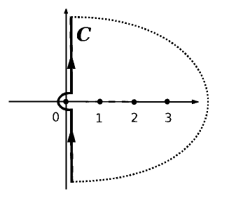
Figure 3: The contours of integration in the complex plane used for summing the series eq.(6.61)

$${\cal S}\bigl{(}{\bf f},{\bf y},{\bf q},\{\eta_{k}\}\bigr{)} = \prod_{\alpha=1}^{M}\Biggl{[}\prod_{k=1}^{N}\Biggl{(}\int_{{\cal C}}dz^{k}_{\alpha}\,\delta(z^{k}_{\alpha})\Biggr{)}-(-1)^{N}\prod_{k=1}^{N}\Biggl{(}\int_{{\cal C}}\frac{dz^{k}_{\alpha}}{2\pi i\,z^{k}_{\alpha}}\exp\Bigl{\{}z^{k}_{\alpha}\bigl{(}y_{\alpha}+f_{k}-\sqrt{\gamma_{k}}\eta_{k}\bigr{)}\Bigr{\}}\Biggr{)}\Biggr{]}$$ (6.62)

$$\times \det\hat{K}\Bigl{[}\bigl{(}\sum_{k}^{N}z^{k}_{\alpha},\;q_{\alpha}\bigr{)};\;\bigl{(}\sum_{k}^{N}z^{k}_{\beta},\;q_{\beta}\bigr{)}\Bigr{]}_{\alpha,\beta=1,...,M}\times\lim_{t\to\infty}G_{M}\Bigl{(}\frac{\kappa{\bf q}}{2\lambda(t)};\;\{\frac{z^{k}_{\alpha}}{\lambda(t)}\}\Bigr{)}$$

Taking into account the Gamma function property $\lim_{|z|\to 0}\Gamma(1+z)=1$ one can easily demonstrate (see e.g. eqs.(5.33) or (6.21)) that

$$\lim_{t\to\infty}G_{M}\Bigl{(}\frac{\kappa{\bf q}}{2\lambda(t)};\;\{\frac{z^{k}_{\alpha}}{\lambda(t)}\}\Bigr{)}\;=\;1$$ (6.63)

Thus in the limit $\lambda\to\infty$ the expression (6.59) takes the form of the Fredholm determinant

$$W({\bf f};{\bf x}) = \sum_{M=0}^{\infty}\frac{(-1)^{M}}{M!}\prod_{\alpha=1}^{M}\Biggl{[}\int\int_{-\infty}^{+\infty}\frac{dq_{\alpha}dy_{\alpha}}{2\pi}\operatorname{Ai}(y_{\alpha}+q_{\alpha}^{2})\prod_{k,l=1}^{N}\Biggl{(}\int_{-\infty}^{+\infty}\frac{d\xi_{kl}^{\alpha}}{\sqrt{2\pi}}\Biggr{)}\prod_{k=1}^{N}\Biggl{(}\int_{-\infty}^{+\infty}\frac{d\eta_{k}^{\alpha}}{\sqrt{2\pi}}\Biggr{)}\times$$ (6.64)

$$\times \exp\Biggl{\{}-\frac{1}{2}\sum_{k,l=1}^{N}\xi_{kl}^{2}-\frac{1}{2}\sum_{k=1}^{N}\Bigl{[}\eta_{k}^{\alpha}+\frac{i}{\sqrt{\gamma_{k}}}\,q_{\alpha}x_{k}+i\sum_{l=1}^{N}\sqrt{\frac{\Delta_{kl}}{2\gamma_{k}}}\;\bigl{(}\xi_{kl}^{\alpha}+\xi_{lk}^{\alpha}\bigr{)}\Bigr{]}^{2}\Biggr{\}}\times$$

$$\times \prod_{k=1}^{N}\Biggl{(}\int_{{\cal C}}dz^{k}_{\alpha}\Biggr{)}\Biggl{(}\prod_{k=1}^{N}\,\delta(z^{k}_{\alpha})\;-\;(-1)^{N}\prod_{k=1}^{N}\frac{1}{2\pi iz^{k}_{\alpha}}\exp\Bigl{\{}z^{k}_{\alpha}\bigl{(}y_{\alpha}+f_{k}-\sqrt{\gamma_{k}}\eta_{k}\bigr{)}\Bigr{\}}\Biggr{)}\Biggr{]}\times$$

$$\times \det\hat{K}\Bigl{[}\bigl{(}\sum_{k}^{N}z^{k}_{\alpha},\;q_{\alpha}\bigr{)};\;\bigl{(}\sum_{k}^{N}z^{k}_{\beta},\;q_{\beta}\bigr{)}\Bigr{]}_{\alpha,\beta=1,...,M}$$

$$\equiv \det\bigl{[}\hat{1}-\hat{A}\bigr{]}\;=\;\exp\Bigl{\{}-\sum_{M=1}^{\infty}\frac{1}{M}\mbox{Tr}\hat{A}^{M}\Bigr{\}}$$ (6.65)

where $\hat{A}$ is the integral operator with the kernel

$$A\Bigl{[}\Bigl{(}\sum_{k}^{N}z^{k},\,q\Bigr{)};\;\Bigl{(}\sum_{k}^{N}\tilde{z}^{k},\,\tilde{q}\Bigr{)}\Bigr{]} = \int_{-\infty}^{+\infty}\frac{dy}{2\pi}\operatorname{Ai}(y+q^{2})\prod_{k,l=1}^{N}\Biggl{(}\int_{-\infty}^{+\infty}\frac{d\xi_{kl}}{\sqrt{2\pi}}\Biggr{)}\prod_{k=1}^{N}\Biggl{(}\int_{-\infty}^{+\infty}\frac{d\eta_{k}}{\sqrt{2\pi}}\Biggr{)}\times$$ (6.66)

$$\times \exp\Biggl{\{}-\frac{1}{2}\sum_{k,l=1}^{N}\xi_{kl}^{2}-\frac{1}{2}\sum_{k=1}^{N}\Bigl{[}\eta_{k}+\frac{i}{\sqrt{\gamma_{k}}}\,q_{\alpha}x_{k}+i\sum_{l=1}^{N}\sqrt{\frac{\Delta_{kl}}{2\gamma_{k}}}\;\bigl{(}\xi_{kl}+\xi_{lk}\bigr{)}\Bigr{]}^{2}\Biggr{\}}\times$$

$$\times \Biggl{(}\prod_{k=1}^{N}\,\delta(z^{k})\;-\;(-1)^{N}\prod_{k=1}^{N}\frac{1}{2\pi iz^{k}}\exp\Bigl{\{}z^{k}\bigl{(}y+f_{k}-\sqrt{\gamma_{k}}\eta_{k}\bigr{)}\Bigr{\}}\Biggr{)}\times$$

$$\times \frac{1}{\sum_{k}^{N}z^{k}\,-\,iq\;+\;\sum_{k}^{N}\tilde{z}^{k}\,+\,i\tilde{q}}$$

Correspondingly, for the trace of this operator in the $M$-th power (in the exponential representation of the Fredholm determinant, eq.(6.65)) we get

$$\mbox{Tr}\hat{A}^{M} = \prod_{\alpha=1}^{M}\Biggl{[}\int\int_{-\infty}^{+\infty}\frac{dydq_{\alpha}}{2\pi}\operatorname{Ai}(y+q_{\alpha}^{2})\prod_{k,l=1}^{N}\Biggl{(}\int_{-\infty}^{+\infty}\frac{d\xi_{kl}}{\sqrt{2\pi}}\Biggr{)}\prod_{k=1}^{N}\Biggl{(}\int_{-\infty}^{+\infty}\frac{d\eta_{k}}{\sqrt{2\pi}}\Biggr{)}\times$$ (6.67)

$$\times \exp\Biggl{\{}-\frac{1}{2}\sum_{k,l=1}^{N}\xi_{kl}^{2}-\frac{1}{2}\sum_{k=1}^{N}\Bigl{[}\eta_{k}+\frac{i}{\sqrt{\gamma_{k}}}\,q_{\alpha}x_{k}+i\sum_{l=1}^{N}\sqrt{\frac{\Delta_{kl}}{2\gamma_{k}}}\;\bigl{(}\xi_{kl}+\xi_{lk}\bigr{)}\Bigr{]}^{2}\Biggr{\}}\times$$

$$\times \prod_{k=1}^{N}\Biggl{(}\int_{{\cal C}}dz^{k}_{\alpha}\Biggr{)}\Biggl{(}\prod_{k=1}^{N}\,\delta(z^{k}_{\alpha})\;-\;(-1)^{N}\prod_{k=1}^{N}\frac{1}{2\pi iz^{k}_{\alpha}}\exp\Bigl{\{}z^{k}_{\alpha}\bigl{(}y+f_{k}-\sqrt{\gamma_{k}}\eta_{k}\bigr{)}\Bigr{\}}\Biggr{)}\Biggr{]}\times$$

$$\times \prod_{\alpha=1}^{M}\Biggl{(}\frac{1}{\sum_{k}^{N}z^{k}_{\alpha}\,-\,iq_{\alpha}\;+\;\sum_{k}^{N}z^{k}_{\alpha+1}\,+\,iq_{\alpha+1}}\Biggr{)}$$

where, by definition, $z^{k}_{M+1}\equiv z^{k}_{1}$ and $q_{M+1}\equiv q_{1}$.

Substituting

$$\frac{1}{\sum_{k}^{N}z^{k}_{\alpha}\,-\,iq_{\alpha}\;+\;\sum_{k}^{N}z^{k}_{\alpha+1}\,+\,iq_{\alpha+1}}\;=\;\int_{0}^{\infty}d\omega_{\alpha}\exp\Bigl{\{}-\omega_{\alpha}\Bigl{(}\sum_{k}^{N}z^{k}_{\alpha}\,-\,iq_{\alpha}\;+\;\sum_{k}^{N}z^{k}_{\alpha+1}\,+\,iq_{\alpha+1}\Bigr{)}\Bigr{\}}$$ (6.68)

into eq.(6.67) we obtain

$$\mbox{Tr}\hat{A}^{M}\;=\;\int_{0}^{\infty}...\int_{0}^{\infty}d\omega_{1}...d\omega_{M}\;\prod_{\alpha=1}^{M}A\bigl{(}\omega_{\alpha};\;\omega_{\alpha+1}\bigr{)}$$ (6.69)

where

$$A\bigl{(}\omega;\;\omega^{\prime}\bigr{)} = \int\int_{-\infty}^{+\infty}\frac{dydq}{2\pi}\operatorname{Ai}(y+q^{2}+\omega+\omega^{\prime})\prod_{k,l=1}^{N}\Biggl{(}\int_{-\infty}^{+\infty}\frac{d\xi_{kl}}{\sqrt{2\pi}}\Biggr{)}\prod_{k=1}^{N}\Biggl{(}\int_{-\infty}^{+\infty}\frac{d\eta_{k}}{\sqrt{2\pi}}\Biggr{)}\times$$ (6.70)

$$\times \exp\Biggl{\{}-\frac{1}{2}\sum_{k,l=1}^{N}\xi_{kl}^{2}-\frac{1}{2}\sum_{k=1}^{N}\Bigl{[}\eta_{k}+\frac{i}{\sqrt{\gamma_{k}}}\,qx_{k}+i\sum_{l=1}^{N}\sqrt{\frac{\Delta_{kl}}{2\gamma_{k}}}\;\bigl{(}\xi_{kl}+\xi_{lk}\bigr{)}\Biggr{]}^{2}-iq(\omega-\omega^{\prime})\Bigr{\}}\times$$

$$\times \Biggl{(}1\;-\;(-1)^{N}\prod_{k=1}^{N}\int_{{\cal C}}\frac{dz^{k}}{2\pi iz^{k}}\exp\Bigl{\{}z^{k}\bigl{(}y+f_{k}-\sqrt{\gamma_{k}}\eta_{k}\bigr{)}\Bigr{\}}\Biggr{)}$$

Integrating over $z^{1},...,z^{N}$ we finally get

$$A\bigl{(}\omega;\;\omega^{\prime}\bigr{)} = \int\int_{-\infty}^{+\infty}\frac{dydq}{2\pi}\operatorname{Ai}(y+q^{2}+\omega+\omega^{\prime})\prod_{k,l=1}^{N}\Biggl{(}\int_{-\infty}^{+\infty}\frac{d\xi_{kl}}{\sqrt{2\pi}}\Biggr{)}\prod_{k=1}^{N}\Biggl{(}\int_{-\infty}^{+\infty}\frac{d\eta_{k}}{\sqrt{2\pi}}\Biggr{)}\times$$ (6.71)

$$\times \exp\Biggl{\{}-\frac{1}{2}\sum_{k,l=1}^{N}\xi_{kl}^{2}-\frac{1}{2}\sum_{k=1}^{N}\Bigl{[}\eta_{k}+\frac{i}{\sqrt{\gamma_{k}}}\,qx_{k}+i\sum_{l=1}^{N}\sqrt{\frac{\Delta_{kl}}{2\gamma_{k}}}\;\bigl{(}\xi_{kl}+\xi_{lk}\bigr{)}\Bigr{]}^{2}-iq(\omega-\omega^{\prime})\Biggr{\}}\times$$

$$\times \Biggl{[}1\;-\;(-1)^{N}\prod_{k=1}^{N}\theta\Bigl{(}-y-f_{k}+\eta_{k}\sqrt{\gamma_{k}}\;\Bigr{)}\Biggr{]}$$

where $\Delta_{kl}=\big{|}x_{k}-x_{l}\big{|}$ and $\gamma_{k}=\sum_{l=1}^{N}\Delta_{kl}$.

Thus the $N$-point free energy distribution function $W\bigl{(}f_{1},...,f_{N};\;x_{1},...,x_{N}\bigr{)}$, eq.(6.39), is given by the Fredholm determinant

$$W\bigl{(}{\bf f};\;{\bf x}\bigr{)}\;=\;\det\bigl{[}\hat{1}\;-\;\hat{A}\bigr{]}$$ (6.72)

where $\hat{A}$ is the integral operator with the kernel $A\bigl{(}\omega;\;\omega^{\prime}\bigr{)}$ (with $\omega,\omega^{\prime}\geq 0$) represented in eq.(6.71).

VII Probability distribution function of the endpoint fluctuations

In this Chapter we consider the problem in which the polymer is fixed at the origin, $\phi(0)=0$ and it is free at $\tau=t$. In other words, for a given realization of the random potential $V$ the partition function of the considered system is:

$$Z(t)=\int_{-\infty}^{+\infty}dx\;Z(x;t)\;=\;\exp\{-\beta F(t)\}$$ (7.1)

where

$$Z(x;t)=\int_{\phi(0)=0}^{\phi(t)=x}{\cal D}\phi(\tau)\;\exp\bigl{\{}-\beta H[\phi;V]\bigr{\}}$$ (7.2)

is the partition function of the system with the fixed boundary condition, $\phi(t)=x$ and $F(t)$ is the total free energy. As it was discussed in the Introduction, besides the usual extensive part $f_{0}t$ (where $f_{0}$ is the linear free energy density), the total free energy $F$ of such system contains the disorder dependent fluctuating contribution $\propto t^{1/3}$. In other words, in the limit of large $t$ the total (random) free energy of the system can be represented as $\beta F(t)=\beta f_{0}t+\lambda(t)f$, where $\lambda(t)=\frac{1}{2}\bigl{(}\beta^{5}u^{2}t\bigr{)}^{1/3}$ and $f\sim 1$ is the random quantity which in the thermodynamic limit $t\to\infty$ is described by the universal Tracy-Widom distribution function $P_{TW}(f)$ (see Chapters IV and V). Note that the trivial self-averaging contribution $f_{0}t$ to the free energy can be eliminated by the simple redefinition of the partition function, $Z=\exp\{-\beta f_{0}t\}\,\tilde{Z}$, so that $\tilde{Z}=\exp\{-\lambda f\}$, (see Chapter II).

In this Chapter instead of the free energy we are going to study on the statistical properties of the transverse fluctuations of the directed polymer itself. The scaling properties of the typical value of the endpoint deviations, $\phi(t)$, at large times is well known: $\overline{\langle\phi(t)\rangle^{2}}\;\propto\;t^{4/3}\;\;$ hhf_85 ; numer1 ; numer2 ; kardar_87 . Much more interesting object is the probability distribution function of the rescaled quantity $x=\phi(t)/t^{2/3}$ which in the limit $t\to\infty$ becomes a universal function math1 ; math2 ; math3 ; end-point ; math4 . This distribution function can be defined as follows:

$$W(x)\;=\;\lim_{t\to\infty}\;\mbox{Prob}\bigl{[}\phi(t)t^{-2/3}\;>\;x\bigr{]}$$ (7.3)

In this Chapter it will be shown that

$$W(x)\;=\;\int_{-\infty}^{+\infty}df\;F_{1}(-f)\int_{0}^{+\infty}d\omega\int_{0}^{+\infty}d\omega^{\prime}\bigl{(}\hat{1}-\hat{K}\bigr{)}^{-1}(\omega,\omega^{\prime})\;\Phi(\omega^{\prime},\omega;\;f,x)$$ (7.4)

Here $\hat{K}$ is the integral operator with the kernel $B(\omega,\omega^{\prime})=\operatorname{Ai}(\omega+\omega^{\prime}-f)\;\;(\omega,\omega^{\prime}\,>\,0)$, the function $F_{1}(-f)=\det\bigl{[}\hat{1}-\hat{K}\bigr{]}$ is the GOE Tracy-Widom distribution (see Chapter V), $\bigl{(}\hat{1}-\hat{K}\bigr{)}^{-1}(\omega,\omega^{\prime})$ denotes the kernel of the inverse operator $\bigl{(}\hat{1}-\hat{K}\bigr{)}^{-1}$ in $\omega$ and $\omega^{\prime}$ and finally the function $\Phi(\omega^{\prime},\omega;\;f,x)$ is:

$$\Phi(\omega,\omega^{\prime};\;f,x)=-\frac{1}{2}\int_{0}^{+\infty}dy\; \Biggl{[} \Bigl{(}\frac{\partial}{\partial\omega}-\frac{\partial}{\partial\omega^{\prime}}\Bigr{)}\Psi\bigl{(}\omega-\frac{1}{2}f+y;\;x\bigr{)}\Psi\bigl{(}\omega^{\prime}-\frac{1}{2}f+y;\;-x\bigr{)}+$$ (7.5)

$$+ \Bigl{(}\frac{\partial}{\partial\omega}+\frac{\partial}{\partial\omega^{\prime}}\Bigr{)}\Psi\bigl{(}\omega-\frac{1}{2}f-y;\;x\bigr{)}\Psi\bigl{(}\omega^{\prime}-\frac{1}{2}f+y;\;-x\bigr{)}\Biggr{]}$$

where

$$\Psi(\omega;x)\;=\;2^{1/3}\mbox{Ai}\Bigl{[}2^{1/3}\bigl{(}\omega+\frac{1}{8}x^{2}\bigr{)}\Bigr{]}\,\exp\bigl{\{}-\frac{1}{2}\omega x\bigr{\}}$$ (7.6)

Unfortunately the above expression for the distribution function is rather complicated and its analytic properties is not so easy to analyze although the asymptotic tail of this function at $|x|\to\infty$ is already known to decay as $\sim\exp\{-|x|^{3}/12\}$ math2 .

In terms of the partition function $\tilde{Z}(x;t)$ the probability distribution function of the polymer’s endpoint $W(x)$, eq.(7.3), can be defined as follows:

$$W(x)\,=\,\lim_{t\to\infty}\,\overline{\Biggl{(}\int_{x}^{+\infty}dx^{\prime}\frac{\tilde{Z}(x^{\prime};t)}{\int_{-\infty}^{+\infty}dx^{\prime}\;\tilde{Z}(x^{\prime};t)}\Biggr{)}}\;=\;\lim_{t\to\infty}\,\overline{\Biggl{(}\frac{\tilde{Z}^{(+)}(x;t)}{\tilde{Z}^{(+)}(x;t)+\tilde{Z}^{(-)}(x;t)}\Biggr{)}}$$ (7.7)

Here, as usual, $\overline{(...)}$ denotes the averaging over the disorder potential and

$$\tilde{Z}^{(-)}(x;t) \equiv \int_{-\infty}^{x}dx^{\prime}\;\tilde{Z}(x^{\prime};t)\;=\;\exp\{-\lambda(t)f_{(-)}\}$$ (7.8)

$$\tilde{Z}^{(+)}(x;t) \equiv \int_{x}^{+\infty}dx^{\prime}\;\tilde{Z}(x^{\prime};t)\;=\;\exp\{-\lambda(t)f_{(+)}\}$$ (7.9)

where $f_{(\pm)}$ are the free energies of the polymers with the endpoint $\phi(t)$ located correspondingly above and below a given position $x$ and

$$\lambda(t)\;=\;\frac{1}{2}\bigl{(}\beta^{5}u^{2}t\bigr{)}^{1/3}\;\propto\;t^{1/3}$$ (7.10)

which implies that the limit $t\to\infty$ is equivalent to the limit $\lambda\to\infty$. According to the above definitions, eqs.(7.8)-(7.9),

$$\lim_{\lambda\to\infty}\;\frac{\exp\{-\lambda f_{(+)}\}}{\exp\{-\lambda f_{(-)}\}\,+\,\exp\{-\lambda f_{(+)}\}}\;=\;\left\{\begin{array}[]{ll}0,\;\;\;\;\mbox{for}\;\;f_{(-)}<f_{(+)}\\ \\ 1,\;\;\;\;\mbox{for}\;\;f_{(-)}>f_{(+)}\end{array}\right.$$ (7.11)

Let us introduce the joint probability density function ${\cal P}_{x}\bigl{[}f_{(+)};f_{(-)}\bigr{]}$ such that the quantity ${\cal P}_{x}\bigl{[}f_{(+)};f_{(-)}\bigr{]}\,df_{(+)}\,df_{(-)}$ gives the probability that the free energy of the polymer with the endpoint located below $x$ is equal to $f_{(-)}$ (within the interval $df_{(-)}$), while the free energy of the polymer with the endpoint located above $x$ is equal to $f_{(+)}$ (within the interval $df_{(+)}$). Thus, according to eq.(7.11),

$$W(x)\;=\;\lim_{\lambda\to\infty}\,\int_{-\infty}^{+\infty}df_{(+)}\int_{f_{(+)}}^{+\infty}df_{(-)}{\cal P}_{x}\bigl{[}f_{(+)};f_{(-)}\bigr{]}$$ (7.12)

Let us introduce one more joint probability distribution function:

$${\cal W}_{x}(f_{1},f_{2})\;=\;\lim_{\lambda\to\infty}\mbox{Prob}\bigl{[}f_{(+)}>f_{1};\;f_{(-)}>f_{2}\bigr{]}\;=\;\lim_{\lambda\to\infty}\int_{f_{1}}^{+\infty}df_{(+)}\int_{f_{2}}^{+\infty}df_{(-)}\,{\cal P}_{x}\bigl{[}f_{(+)};f_{(-)}\bigr{]}$$ (7.13)

This two-point free energy distribution function gives the probability that the free energy of the polymer with the endpoint located above the position $x$ is bigger than a given value $f_{1}$, while the free energy of the polymer with the endpoint located below the position $x$ is bigger than a given value $f_{2}$. According to this definition,

$${\cal P}_{x}\bigl{[}f_{1};f_{2}\bigr{]}\;=\;\frac{\partial}{\partial f_{1}}\,\frac{\partial}{\partial f_{2}}\,{\cal W}_{x}(f_{1},f_{2})$$ (7.14)

Substituting this relation into eq.(7.11) we find

$$W(x)\;=\;\lim_{\lambda\to\infty}\int_{-\infty}^{+\infty}df_{1}\int_{f_{1}}^{+\infty}df_{2}\frac{\partial}{\partial f_{1}}\,\frac{\partial}{\partial f_{2}}\,{\cal W}_{x}(f_{1},f_{2})$$ (7.15)

Integrating by parts over $f_{2}$ and taking into account that ${\cal W}_{x}(f_{1},f_{2})\big{|}_{f_{2}=+\infty}=0$ we get

$$W(x)\;=\;\lim_{\lambda\to\infty}-\int_{-\infty}^{+\infty}df_{1}\Bigl{(}\frac{\partial}{\partial f_{1}}\,{\cal W}_{x}(f_{1},f_{2})\Bigr{)}\Big{|}_{f_{2}=f_{1}+0}$$ (7.16)

Thus, to get the distribution function $W(x)$ for the polymer’s endpoint fluctuations we have to derive the two-point free energy distribution function ${\cal W}_{x}(f_{1},f_{2})$ first. Note that this function is different from the two-point free energy distribution function derived in Chapter VI which describes joint statistics of the free energies of the directed polymers coming to two given endpoints.

According to the definition, eq.(7.12), the probability distribution function $V_{x}(f_{1},f_{2})$ can be defined as follows:

$${\cal W}_{x}(f_{1},f_{2})=\lim_{\lambda\to\infty}\sum_{L=0}^{\infty}\sum_{R=0}^{\infty}\frac{(-1)^{L}}{L!}\frac{(-1)^{R}}{R!}\exp\bigl{\{}\lambda Lf_{1}+\lambda Rf_{2}\bigr{\}}\;\overline{\bigl{[}Z^{(+)}(x)\bigr{]}^{L}\,\bigl{[}Z^{(-)}(x)\bigr{]}^{R}}$$ (7.17)

Substituting eqs.(7.7)-(7.8) into eq.(7.17) we get:

$${\cal W}_{x}(f_{1},f_{2})=\lim_{\lambda\to\infty}\sum_{L,R=0}^{\infty}\frac{(-1)^{L+R}}{L!R!}\exp\bigl{\{}\lambda Lf_{1}+\lambda Rf_{2}\bigr{\}}\;\int_{-\infty}^{x}dx_{1}...dx_{L}\int_{x}^{+\infty}dy_{1}...dy_{R}\Psi(x_{1},...,x_{L},y_{R},...,y_{1};t)$$ (7.18)

where the wave function

$$\Psi(x_{1},...,x_{N};t)\;\equiv\;\overline{Z(x_{1})\,Z(x_{2})\,...\,Z(x_{N})}$$ (7.19)

is given in eqs.(3.15)-(3.16).

Further calculations of ${\cal W}_{x}(f_{1},f_{2})$, eq.(7.18) to a large extent repeats the procedure described in detail in the Chapter V for the GOE Tracy-Widom free energy distribution function. The only two differences of the present procedure from the one in Chapter V are: (1) instead of the exponential factor $\lambda Nf\;=\;\lambda(K+L)f$ in the expression for the probability function $W(f)$ eq.(2.19), we now have the factor $\lambda Lf_{1}+\lambda Rf_{2}$ in eq.(7.18); (2) in the integrations over $x_{a}$’s and $y_{a}$’s the regions $(-\infty;0]$ and $[0;+\infty)$ in eqs.(5.7) and (5.11) are changed correspondingly for $(-\infty;x]$ and $[x;+\infty)$ in eq.(7.18) Following the steps given in eqs.(5.7)-(5.15) instead of eq.(LABEL:5.16) get

$${\cal W}_{x}(f_{1},f_{2}) = \lim_{\lambda\to\infty}\sum_{L,R=0}^{\infty}\;(-1)^{L+R}\;\exp\bigl{\{}\lambda Lf_{1}+\lambda Rf_{2}\bigr{\}}\times$$

$$\times \sum_{M=1}^{\infty}\frac{1}{M!}\prod_{\alpha=1}^{M}\Biggl{[}\sum_{n_{\alpha}=1}^{\infty}\,\int_{-\infty}^{+\infty}\frac{dq_{\alpha}\,\kappa^{n_{\alpha}}}{2\pi}\exp\Bigl{\{}-\frac{t}{2\beta}\,n_{\alpha}q_{\alpha}^{2}\,+\,\frac{\kappa^{2}\,t}{24\beta}n_{\alpha}^{3}\Bigr{\}}\Biggr{]}D_{M}({\bf q},{\bf n})J_{L,R}({\bf q},{\bf n};\,x)\;\,{\boldsymbol{\delta}}\Bigl{(}\sum_{\alpha=1}^{M}n_{\alpha},K+L\Bigr{)}$$

where

$$D_{M}({\bf q},{\bf n})\;=\;\det\Biggl{[}\frac{1}{\frac{1}{2}\kappa n_{\alpha}-iq_{\alpha}+\frac{1}{2}\kappa n_{\beta}+iq_{\beta}}\Biggr{]}_{\alpha,\beta=1,...M}$$ (7.21)

and (s.f. eq.(5.15))

$$J_{L,R}({\bf q},{\bf n};\,x) = i^{-(L+R)}\;\exp\bigl{\{}ix\sum_{\alpha=1}^{M}n_{\alpha}q_{\alpha}\bigr{\}}\sum_{{\cal P}^{(L,R)}}\;\;\prod_{a=1}^{L}\prod_{c=1}^{R}\Biggl{[}\frac{q_{{\cal P}_{a}^{(L)}}-q_{{\cal P}_{c}^{(R)}}-i\kappa}{q_{{\cal P}_{a}^{(L)}}-q_{{\cal P}_{c}^{(R)}}}\Biggr{]}\times$$ (7.22)

$$\times \frac{1}{\prod_{a=1}^{L}q^{(-)}_{{\cal P}_{a}^{(L)}}}\prod_{a<b}^{L}\Biggl{[}\frac{q^{(-)}_{{\cal P}_{a}^{(L)}}+q^{(-)}_{{\cal P}_{b}^{(L)}}+i\kappa}{q^{(-)}_{{\cal P}_{a}^{(L)}}+q^{(-)}_{{\cal P}_{b}^{(L)}}}\Biggr{]}\times\frac{(-1)^{R}}{\prod_{c=1}^{R}q^{(+)}_{{\cal P}_{c}^{(R)}}}\prod_{c<d}^{R}\Biggl{[}\frac{q^{(+)}_{{\cal P}_{c}^{(R)}}+q^{(+)}_{{\cal P}_{d}^{(R)}}-i\kappa}{q^{(+)}_{{\cal P}_{c}^{(R)}}+q^{(+)}_{{\cal P}_{d}^{(R)}}}\Biggr{]}$$

The only difference of the above expression for $J_{L,R}({\bf q},{\bf n};\,x)$ from $I_{L,R}({\bf q},{\bf n})$ , eq.(5.15), is the presence of the additional factor $\exp\bigl{\{}ix\sum_{\alpha=1}^{M}n_{\alpha}q_{\alpha}\bigr{\}}$. Following the derivation given in eqs.(5.17)-(5.23) we obtain

$${\cal W}_{x}(f_{1},f_{2}) = \lim_{\lambda\to\infty}\sum_{M=0}^{\infty}\;\frac{(-1)^{M}}{M!}\;\prod_{\alpha=1}^{M}\Biggl{[}\int\int_{-\infty}^{+\infty}\frac{dy_{\alpha}dp_{\alpha}}{2\pi}\operatorname{Ai}\bigl{(}y_{\alpha}+p_{\alpha}^{2}-ixp_{\alpha}\bigr{)}\sum_{m_{\alpha}+s_{\alpha}\geq 1}^{\infty}(-1)^{m_{\alpha}+s_{\alpha}-1}\times$$ (7.23)

$$\times \exp\Bigl{\{}\lambda m_{\alpha}(y_{\alpha}+f_{1})+\lambda s_{\alpha}(y_{\alpha}+f_{2})\Bigr{\}}\;{\cal G}\Bigl{(}\frac{p_{\alpha}}{\lambda},\;m_{\alpha},\;s_{\alpha}\Bigr{)}\;\Biggr{]}\times$$

$$\times \det\hat{K}\bigl{[}(\lambda m_{\alpha},\,\lambda s_{\alpha},\,p_{\alpha});(\lambda m_{\beta},\,\lambda s_{\beta},\,p_{\beta})\bigr{]}_{\alpha,\beta=1,...,M}\;{\bf G}_{M}\Bigl{(}\frac{{\bf p}}{\lambda},\;{\bf m},\;{\bf s}\Bigr{)}\Biggr{\}}$$

where

$$\hat{K}\bigl{[}(\lambda m,\,\lambda s,\,p);(\lambda m^{\prime},\,\lambda s^{\prime},\,p^{\prime})\bigr{]}\;=\;\frac{1}{\lambda m+\lambda s-ip+\lambda m^{\prime}+\lambda s^{\prime}+ip^{\prime}}$$ (7.24)

and the explicit expression for the factors ${\cal G}\bigl{(}\frac{p_{\alpha}}{\lambda},m_{\alpha},s_{\alpha}\bigr{)}$ and ${\cal G}_{\alpha\beta}\bigl{(}{\bf q},\;{\bf m},\;{\bf s}\bigr{)}$ are given in eqs.(5.24) and (E.18) correspondingly. Performing summations over $\{m_{\alpha}\}$ and $\{s_{\alpha}\}$ (see eq.(5.25)-(5.33)) in the limit $\lambda\to\infty$ we find that the expression for the probability function, eq.(7.23) takes the form of the Fredholm determinant (s.f. eq.(5.34))

$${\cal W}_{x}(f_{1},f_{2}) = 1+\sum_{M=1}^{\infty}\;\frac{(-1)^{M}}{M!}\;\prod_{\alpha=1}^{M}\Biggl{[}\int\int_{-\infty}^{+\infty}\frac{dy_{\alpha}dp_{\alpha}}{2\pi}\operatorname{Ai}\bigl{(}y_{\alpha}+p_{\alpha}^{2}-ixp_{\alpha}\bigr{)}\times$$ (7.25)

$$\times \int\int_{{\cal C}^{\prime}}\frac{d{z_{1}}_{\alpha}d{z_{2}}_{\alpha}}{(2\pi i)^{2}}\Bigl{(}\frac{2\pi i}{{z_{1}}_{\alpha}}\delta({z_{2}}_{\alpha})+\frac{2\pi i}{{z_{2}}_{\alpha}}\delta({z_{1}}_{\alpha})-\frac{1}{{z_{1}}_{\alpha}{z_{2}}_{\alpha}}\Bigr{)}\Bigl{(}1+\frac{{z_{1}}_{\alpha}}{{z_{2}}_{\alpha}+ip_{\alpha}^{(-)}}\Bigr{)}\Bigl{(}1+\frac{{z_{2}}_{\alpha}}{{z_{1}}_{\alpha}-ip_{\alpha}^{(+)}}\Bigr{)}\times$$

$$\times \exp\Bigl{\{}{z_{1}}_{\alpha}\bigl{(}y_{\alpha}+f_{1}\bigr{)}+{z_{2}}_{\alpha}\bigl{(}y_{\alpha}+f_{2}\bigr{)}\Bigr{\}}\Biggr{]}\det\Bigl{[}\frac{1}{{z_{1}}_{\alpha}+{z_{2}}_{\alpha}-ip_{\alpha}+{z_{1}}_{\beta}+{z_{2}}_{\beta}+ip_{\beta}}\Bigr{]}_{(\alpha,\beta)=1,2,...,M}$$

$$= \det\bigl{[}\hat{1}\,-\,\hat{B}\bigr{]}$$

with the kernel (s.f. eq.(5.35))

$$\hat{B}\bigl{[}({z_{1}},\,{z_{2}},\,p);({z_{1}}^{\prime},\,{z_{2}}^{\prime},\,p^{\prime})\bigr{]} = \int_{-\infty}^{+\infty}\frac{dy}{2\pi}\operatorname{Ai}\bigl{(}y+p^{2}-ixp\bigr{)}\Bigl{(}\frac{2\pi i}{z_{1}}\delta(z_{2})+\frac{2\pi i}{z_{2}}\delta(z_{1})-\frac{1}{z_{1}{z_{2}}}\Bigr{)}\times$$ (7.26)

$$\times \Bigl{(}1+\frac{z_{1}}{z_{2}+ip^{(-)}}\Bigr{)}\Bigl{(}1+\frac{z_{2}}{z_{1}-ip^{(+)}}\Bigr{)}\exp\Bigl{\{}z_{1}\bigl{(}y+f_{1}\bigr{)}+z_{2}\bigl{(}y+f_{2}\bigr{)}\Bigr{\}}\times$$

$$\times \frac{1}{{z_{1}}+{z_{2}}-ip+{z_{1}}^{\prime}+{z_{2}}^{\prime}+ip^{\prime}}$$

In the exponential representation of this determinant we get

$${\cal W}_{x}(f_{1},f_{2})\;=\;\exp\Bigl{[}-\sum_{M=1}^{\infty}\frac{1}{M}\;\mbox{Tr}\,\hat{B}^{M}\Bigr{]}$$ (7.27)

where

$$\mbox{Tr}\,\hat{B}^{M} = \prod_{\alpha=1}^{M}\Biggl{[}\int\int_{-\infty}^{+\infty}\frac{dy_{\alpha}dp_{\alpha}}{2\pi}\operatorname{Ai}\bigl{(}y_{\alpha}+p_{\alpha}^{2}-ixp_{\alpha}\bigr{)}\times$$ (7.28)

$$\times \int\int_{{\cal C}^{\prime}}\frac{d{z_{1}}_{\alpha}d{z_{2}}_{\alpha}}{(2\pi i)^{2}}\Bigl{(}\frac{2\pi i}{{z_{1}}_{\alpha}}\delta({z_{2}}_{\alpha})+\frac{2\pi i}{{z_{2}}_{\alpha}}\delta({z_{1}}_{\alpha})-\frac{1}{{z_{1}}_{\alpha}{z_{2}}_{\alpha}}\Bigr{)}\Bigl{(}1+\frac{{z_{1}}_{\alpha}}{{z_{2}}_{\alpha}+ip_{\alpha}^{(-)}}\Bigr{)}\Bigl{(}1+\frac{{z_{2}}_{\alpha}}{{z_{1}}_{\alpha}-ip_{\alpha}^{(+)}}\Bigr{)}\times$$

$$\times \exp\Bigl{\{}{z_{1}}_{\alpha}\bigl{(}y_{\alpha}+f_{1}\bigr{)}+{z_{2}}_{\alpha}\bigl{(}y_{\alpha}+f_{2}\bigr{)}\Bigr{\}}\Biggr{]}\;\prod_{\alpha=1}^{M}\Biggl{[}\frac{1}{{z_{1}}_{\alpha}+{z_{2}}_{\alpha}-ip_{\alpha}+{z_{1}}_{\alpha+1}+{z_{2}}_{\alpha+1}+ip_{\alpha+1}}\Biggr{]}$$

Here, by definition, it is assumed that ${z_{i_{M+1}}}\equiv{z_{i_{1}}}$ ($i=1,2$) and $p_{M+1}\equiv p_{1}$. Substituting

$$\frac{1}{{z_{1}}_{\alpha}+{z_{2}}_{\alpha}-ip_{\alpha}+{z_{1}}_{\alpha+1}+{z_{2}}_{\alpha+1}+ip_{\alpha+1}}\;=\;\int_{0}^{\infty}d\omega_{\alpha}\exp\Bigl{[}-\bigl{(}{z_{1}}_{\alpha}+{z_{2}}_{\alpha}-ip_{\alpha}+{z_{1}}_{\alpha+1}+{z_{2}}_{\alpha+1}+ip_{\alpha+1}\bigr{)}\,\omega_{\alpha}\Bigr{]}$$ (7.29)

into eq.(7.28), we obtain

$$\mbox{Tr}\,\hat{B}^{M}\;=\;\int_{0}^{\infty}d\omega_{1}\,...\,d\omega_{M}\,\prod_{\alpha=1}^{M}\Biggl{[}\int\int_{-\infty}^{+\infty}\frac{dydp}{2\pi}\operatorname{Ai}\bigl{(}y+p^{2}+\omega_{\alpha}+\omega_{\alpha-1}-ixp\bigr{)}\exp\{ip\bigl{(}\omega_{\alpha}-\omega_{\alpha-1}\bigr{)}\}\;S\bigl{(}p,y;f_{1},f_{2}\bigr{)}\Biggr{]}$$ (7.30)

where, by definition, $\omega_{0}\equiv\omega_{M}$, and

$$S(p,y;f_{1},f_{2}) = \int\int_{{\cal C}^{\prime}}\frac{dz_{1}dz_{2}}{(2\pi i)^{2}}\Bigl{(}\frac{2\pi i}{z_{1}}\delta(z_{2})+\frac{2\pi i}{z_{2}}\delta(z_{1})-\frac{1}{z_{1}z_{2}}\Bigr{)}\Bigl{(}1+\frac{z_{1}}{z_{2}+ip^{(-)}}\Bigr{)}\Bigl{(}1+\frac{z_{2}}{z_{1}-ip^{(+)}}\Bigr{)}\times$$ (7.31)

$$\times \exp\Bigl{\{}z_{1}\bigl{(}y+f_{1}\bigr{)}+z_{2}\bigl{(}y+f_{2}\bigr{)}\Bigr{\}}$$

Simple integrations yields the following result:

$$S(p,y;f_{1},f_{2}) = \theta(y+f_{1})+\theta(y+f_{2})-\theta(y+f_{1})\theta(y+f_{2})-\theta(y+f_{1})\theta(y+f_{2})\exp\bigl{\{}ip(f_{1}-f_{2})-2\epsilon y\bigr{\}}$$ (7.32)

$$+ \frac{i}{p+i\epsilon}\delta(y+f_{2})-\frac{i}{p-i\epsilon}\delta(y+f_{1})$$

$$- \frac{i}{p+i\epsilon}\delta(y+f_{2})\theta(f_{1}-f_{2})\Bigl{[}1-\exp\{i(p+i\epsilon)(f_{1}-f_{2})\}\Bigr{]}$$

$$+ \frac{i}{p-i\epsilon}\delta(y+f_{1})\theta(f_{2}-f_{1})\bigl{[}1-\exp\{i(p-i\epsilon)(f_{1}-f_{2})\}\bigr{]}$$

According to eq.(7.16) in what follows we will be dealing with the sector $f_{2}>f_{1}$ only. In this case the above expression simplifies to

$$S(p,y;f_{1},f_{2})\big{|}_{f_{2}>f_{1}} = \Bigl{(}\frac{i}{p+i\epsilon}-\frac{i}{p-i\epsilon}\Bigr{)}\delta(y+f_{2})$$ (7.33)

$$+ \frac{i}{p-i\epsilon}\Bigl{[}\delta(y+f_{2})-\delta(y+f_{1})\exp\{ip(f_{1}-f_{2})\}\Bigr{]}$$

$$+ \theta(y+f_{2})-\theta(y+f_{1})\exp\{ip(f_{1}-f_{2})-2\epsilon y\}$$

Note that at edge of the sector $f_{2}>f_{1}$ in the limit $\epsilon\to 0$

$$S(p,y;f_{1},f_{2})\big{|}_{f_{2}=f_{1}+0}\;=\;2\pi\delta(p)\delta(y+f_{2})$$ (7.34)

Substituting eq.(7.33)) into eq.(7.30), we find that the free energy distribution function ${\cal W}_{x}(f_{1},f_{2})$, eq.(7.13), (in the sector $f_{2}>f_{1}$) is given by the Fredholm determinant, eq.(7.27), with the kernel

$$B(\omega,\omega^{\prime}) = \operatorname{Ai}(\omega+\omega^{\prime}-f_{2})-$$ (7.35)

$$- \int_{-\infty}^{+\infty}\frac{dp}{2\pi}\frac{\Bigl{[}\operatorname{Ai}(\omega+\omega^{\prime}+p^{2}-ipx-f_{2})-\operatorname{Ai}(\omega+\omega^{\prime}+p^{2}-ipx-f_{1})\exp\{ip(f_{1}-f_{2})\}\Bigr{]}}{i(p-i\epsilon)}\exp\{ip\bigl{(}\omega-\omega^{\prime}\bigr{)}\}+$$

$$+ \int_{-\infty}^{+\infty}\frac{dp}{2\pi}\Biggl{[}\int_{-f_{2}}^{+\infty}dy\operatorname{Ai}(\omega+\omega^{\prime}+p^{2}-ipx+y)-\int_{-f_{1}}^{+\infty}dy\operatorname{Ai}(\omega+\omega^{\prime}+p^{2}-ipx+y)\exp\{ip(f_{1}-f_{2})\}\Biggr{]}\times$$

$$\times \exp\{ip\bigl{(}\omega-\omega^{\prime}\bigr{)}\}$$

with $\omega,\omega^{\prime}>0$.

Finally, substituting the above result, eqs.(7.27) and (7.35), into eq.(7.16) for the endpoint distribution function one obtains the following expression:

$$W(x)\;=\;\int_{-\infty}^{+\infty}df\;F_{1}(-f)\int_{0}^{+\infty}d\omega\int_{0}^{+\infty}d\omega^{\prime}\Bigl{(}\hat{1}-\hat{K}\Bigr{)}^{-1}(\omega,\omega^{\prime})\;\Phi(\omega^{\prime},\omega;f,x)$$ (7.36)

where

$$F_{1}(-f)=\det\bigl{[}\hat{1}\,-\,\hat{K}\bigr{]}\;=\;\exp\Bigl{[}-\sum_{M=1}^{\infty}\frac{1}{M}\;\mbox{Tr}\,\hat{K}^{M}\Bigr{]}$$ (7.37)

is the GOE Tracy-Widom distribution with the kernel

$$K(\omega,\omega^{\prime})\;=\;\operatorname{Ai}(\omega+\omega^{\prime}-f),\;\;\;\;\;\;\;(\omega,\omega^{\prime}\,>\,0)$$ (7.38)

(see eqs.(5.3)-(5.5)) and

$$\Phi(\omega,\omega^{\prime};f,x) = i\int_{-\infty}^{+\infty}\frac{dp}{2\pi}\;\frac{1}{p-i\epsilon}\;\operatorname{Ai}^{\prime}(\omega+\omega^{\prime}+p^{2}-ipx-f)\;\exp\{ip\bigl{(}\omega-\omega^{\prime}\bigr{)}\}$$ (7.39)

$$- i\int_{-f}^{+\infty}dy\;\int_{-\infty}^{+\infty}\frac{dp}{2\pi}\,p\,\operatorname{Ai}(\omega+\omega^{\prime}+p^{2}-ipx+y)\;\exp\{ip\bigl{(}\omega-\omega^{\prime}\bigr{)}\}$$

Using the standard integral representation of the Airy function (see Appendix B) one can easily reduce the above function $\Phi(\omega,\omega^{\prime};f,x)$ to the following more simple form:

$$\Phi(\omega,\omega^{\prime};f,x)=-\frac{1}{2}\int_{0}^{+\infty}dy\; \Biggl{[} \Bigl{(}\frac{\partial}{\partial\omega}-\frac{\partial}{\partial\omega^{\prime}}\Bigr{)}\Psi\bigl{(}\omega-\frac{1}{2}f+y;\;x\bigr{)}\Psi\bigl{(}\omega^{\prime}-\frac{1}{2}f+y;\;-x\bigr{)}+$$ (7.40)

$$+ \Bigl{(}\frac{\partial}{\partial\omega}+\frac{\partial}{\partial\omega^{\prime}}\Bigr{)}\Psi\bigl{(}\omega-\frac{1}{2}f-y;\;x\bigr{)}\Psi\bigl{(}\omega^{\prime}-\frac{1}{2}f+y;\;-x\bigr{)}\Biggr{]}$$

where

$$\Psi(\omega;x)\;=\;2^{1/3}\mbox{Ai}\Bigl{[}2^{1/3}\bigl{(}\omega+\frac{1}{8}x^{2}\bigr{)}\Bigr{]}\,\exp\bigl{\{}-\frac{1}{2}\omega x\bigr{\}}$$ (7.41)

Thus, eqs.(7.36)-(7.41) complete the derivation of the probability distribution function for the directed polymer’s endpoint. Unfortunately, we see that at present stage this final expression is rather involved, so that the study of its analytical properties requires special efforts.

PART 2: Unsolved problems

VIII Zero temperature limit

In this Chapter we will study the statistical properties of one-dimensional directed polymers in correlated random potential in the zero-temperature limit. This system is defined in terms of the Hamiltonian

$$H[\phi(\tau),V]=\int_{0}^{t}d\tau\Bigl{\{}\frac{1}{2}\bigl{[}\partial_{\tau}\phi(\tau)\bigr{]}^{2}+V[\phi(\tau),\tau]\Bigr{\}};$$ (8.1)

where $V(\phi,\tau)$ is the Gaussian distributed random potential with a zero mean, $\overline{V(\phi,\tau)}=0$, and the correlation function

$$\overline{V(\phi,\tau)V(\phi^{\prime},\tau^{\prime})}=u\delta(\tau-\tau^{\prime})U(\phi-\phi^{\prime})$$ (8.2)

Here $U(\phi)$ is the ”spatial” correlation function characterized by some finite correlation length $R$. For simplicity we take

$$U(\phi)\;=\;\frac{1}{\sqrt{2\pi}\,R}\;\exp\Bigl{\{}-\frac{\phi^{2}}{2R^{2}}\Bigr{\}}$$ (8.3)

It can be argued (see below) that the model, eqs.(8.1)-(8.3), with finite correlation length $R$ in the high temperature limit is equivalent to the one with the $\delta$-correlated random potentials considered in the previous chapters. Note that this provides the basis for the short-length regularization of the model with the $\delta$-potentials which, in fact, is ill defined at short scales. The zero-temperature limit for this model is much less clear. The problem is that in the exact solution of the model with $\delta$-correlated potentials (Chapter IV) the fluctuating part of the free energy $F(T,t)$ (in the limit $t\to\infty$) is proportional to $(u/T)^{2/3}\,t^{1/3}\,f$ and this free energy does not reveal any finite zero-temperature limit. The physical origin of this pathology is clear: the exact solution mentioned above is valid only for the model with $\delta$-correlated potentials which is ill defined at short scales while it is the short scales which are getting the most relevant in the limit $T\to 0$. One can propose two types of the regularization of the model on short scales: (1) introducing a lattice, and (2) keeping continuous structure of the ”space-time” but introducing smooth finite size correlations for the random potential like in eq.(8.3). In both cases, however, the solution derived for the model with $\delta$-correlated potentials becomes not valid. Nevertheless, it is generally believed that in the zero-temperature limit the considered system must reveal the same TW distribution. On one hand there are exact results for strictly zero temperature lattice models revealing main features of (1+1) directed polymers (see e.g rigorous solution of the directed polymer lattice model with geometric disorder Johansson ). On the other hand there are analytic indications that in the zero-temperature limit the continuous model with finite correlation length of the type introduced above, eqs.(8.1)-(8.3), after crossover to a new regime keeps the main features of the finite-temperature solution Korshunov ; Lecomte .

In this Chapter we will try to formulate a general scheme which would allow to obtain a finite zero-temperature limit for the continuous model (8.1)-(8.3). In terms of the standard replica technique (see Chapters II and III) it will be demonstrated that in the limit $T\to 0$ the considered system reveals the one-step replica symmetry breaking structure similar to the one which takes place in the low-temperature phase of the Random Energy Model (REM) REM . Of course, the considered system (unlike REM) reveal no phase transition: here at the temperature $T_{*}\sim(uR)^{1/3}$ we observe only a crossover from the high- to the low-temperature regime. Namely, at $T\gg T_{*}$ the fluctuating part of the free energy is the same as in the model with the $\delta$-interactions, $F(T,t)\simeq(u/T)^{2/3}\,t^{1/3}\,f$, while at $T\ll T_{*}$ the non-universal prefactor of the free energy saturates at finite value, $F(T=0,t)\simeq(u^{2}/R)^{1/9}\,t^{1/3}\,f$. The probability distribution function of the random quantity $f$ is, of course, expected to be the TW one, although at present stage this is not proved yet.

For simplicity let us consider the case of the zero boundary conditions: $\phi(0)=\phi(t)=0$. Following the procedure described in Chapters II and III, the free energy probability distribution function $P(F)$ of this system can be studied in terms of the replica partition function:

$$Z(N,t)\;=\;\int_{-\infty}^{+\infty}dF\,P(F)\,\exp\bigl{\{}-\beta NF\bigr{\}}$$ (8.4)

where

$$Z(N,t)\;=\;\prod_{a=1}^{N}\int_{\phi_{a}(0)=0}^{\phi_{a}(t)=0}{\cal D}\phi_{a}(\tau)\;\exp\Bigl{\{}-\beta H_{N}[\boldsymbol{\phi}(\tau)]\Bigr{\}}$$ (8.5)

with the replica Hamiltonian

$$\beta H_{N}[\boldsymbol{\phi}]=\int_{0}^{t}d\tau\Biggl{[}\frac{1}{2}\beta\sum_{a=1}^{N}\Bigl{(}\partial_{\tau}\phi_{a}(\tau)\Bigr{)}^{2}\;-\;\frac{1}{2}\beta^{2}\,u\,\sum_{a,b=1}^{N}U\bigl{(}\phi_{a}(\tau)-\phi_{b}(\tau)\bigr{)}\Biggr{]};$$ (8.6)

which describes $N$ elastic strings $\bigl{\{}\phi_{1}(\tau),\,\phi_{2}(\tau),\,...\,,\phi_{N}(\tau)\bigr{\}}$ with the finite width attractive interactions $U\bigl{(}\phi_{a}-\phi_{b}\bigr{)}$, eq.(8.3).

Mapping this system to the $N$-particle quantum boson model (see Chapter III) one introduces the wave function

$$\Psi(x_{1},\,x_{2},\,...\,x_{N};\;t)\;=\;\prod_{a=1}^{N}\int_{\phi_{a}(0)=0}^{\phi_{a}(t)=x_{a}}{\cal D}\phi_{a}(\tau)\;\exp\Bigl{\{}-\beta H_{N}[\boldsymbol{\phi}(\tau)]\Bigr{\}}$$ (8.7)

such that $Z(N,t)\,=\,\Psi(x_{1},x_{2},...x_{N};\,t)\big{|}_{x_{a}=0}$. The above wave function can be obtained as the solution of the the imaginary time Schrödinger equation

$$\beta\frac{\partial}{\partial t}\Psi({\bf x};\,t)\;=\;\frac{1}{2}\sum_{a=1}^{N}\,\frac{\partial^{2}}{\partial x_{a}^{2}}\Psi({\bf x};\,t)\;+\;\frac{1}{2}\,\beta^{3}u\,\sum_{a,b=1}^{N}U(x_{a}-x_{b})\,\Psi({\bf x};\,t)$$ (8.8)

with the initial condition $\Psi({\bf x};\,0)\;=\;\prod_{a=1}^{N}\,\delta(x_{a})$. In the high temperature limit ($\beta\to 0$) the typical distance between the particles (defined by the wave function $\Psi({\bf x};\,t)$) is much larger that the size $R$ of the potential $U(x)$, eq.(8.3) (see below). In this case the potential $U(x)$ can be approximated by the $\delta$-function, so that a generic solution of the Schrödinger equation (8.9) (with $U(x)=\delta(x)$) is obtained in terms of the Bethe ansatz eigenfunctions, eqs.(3.13)-(3.19). In particular, the ground state wave function (which in eqs.(3.13)-(3.15) corresponds to $M=1;\;Q_{a}=q-\frac{i}{2}\kappa(N+1-2a)$) of this system is:

$$\Psi_{q}({\bf x})\;\propto\;\exp\Bigl{\{}-\frac{1}{4}\,\kappa\sum_{a,b=1}^{N}|x_{a}-x_{b}|\,+\,iq\sum_{a=1}^{N}x_{a}\Bigr{\}}$$ (8.9)

For the excited states (with $M>1$) the generic wave function can be represented as a linear combination of various products of the ”cluster” wave functions which have the structure similar to the one in eq.(8.9). We see that in any case the typical distance between the particles is of the order of $\kappa^{-1}\,=\,(\beta^{3}u)^{-1}$. Thus, the approximation of the potential $U(x)$, eq.(8.3), by the $\delta$-function is justified provided $(\beta^{3}u)^{-1}\gg R$ which for a given $R$ and $u$ is valid only in the high temperature region,

$$\beta\,\ll\,(Ru)^{-1/3}$$ (8.10)

At temperatures of the order of the $(Ru)^{1/3}$ and below the typical distance between particles becomes comparable with the size $R$ of the potential $U(x)$, and therefore its approximation by the $\delta$-function is no longer valid, which makes the considered model unsolvable (at least for the time being). It turns out, however, that in the zero temperature limit, at $T\ll(Ru)^{1/3}$ the situation somewhat simplifies again (see below).

One can easily show that the parameters of the considered system can be redefined in such a way that in the limit $t\to\infty$ the properties of the system would depend on the only parameter, which is the reduced temperature $\tilde{T}\,=\,T/T_{*}$ where

$$T_{*}\,=\,\Bigl{(}\frac{uR}{\sqrt{2\pi}}\Bigr{)}^{1/3}$$ (8.11)

Indeed, redefining

$$\phi \to R\,\phi$$

$$\beta = T_{*}^{-1}\,\tilde{\beta}$$ (8.12)

$$\tau \to \tau_{*}\,\tau$$

with

$$\tau_{*}\,=\,\Bigl{(}\sqrt{2\pi}\,R^{5}u^{-1}\Bigr{)}^{1/3}$$ (8.13)

instead of the replica Hamiltonian, eq.(8.6), one gets

$$\beta\tilde{H}_{N}[\boldsymbol{\phi}]=\int_{0}^{t/\tau_{*}}d\tau\Biggl{[}\frac{1}{2}\,\tilde{\beta}\sum_{a=1}^{N}\Bigl{(}\partial_{\tau}\phi_{a}(\tau)\Bigr{)}^{2}\;-\;\frac{1}{2}\,\tilde{\beta}^{2}\sum_{a,b=1}^{N}U_{0}\bigl{(}\phi_{a}(\tau)-\phi_{b}(\tau)\bigr{)}\Biggr{]};$$ (8.14)

where

$$U_{0}(\phi)\;=\;\exp\Bigl{\{}-\frac{1}{2}\,\phi^{2}\Bigr{\}}$$ (8.15)

Accordingly, the wave function $\tilde{\Psi}({\bf x};t)$ defined by eq.(8.7) with $\beta H_{N}[\boldsymbol{\phi}]$ replaced by $\beta\tilde{H}_{N}[\boldsymbol{\phi}]$ is given by the solution of the Schrödinger equation

$$2\tilde{\beta}\frac{\partial}{\partial\tilde{t}}\tilde{\Psi}({\bf x};\,\tilde{t})\;=\;\sum_{a=1}^{N}\,\frac{\partial^{2}}{\partial x_{a}^{2}}\tilde{\Psi}({\bf x};\,\tilde{t})\;+\;{\tilde{\beta}}^{3}\sum_{a,b=1}^{N}U_{0}(x_{a}-x_{b})\,\tilde{\Psi}({\bf x};\,\tilde{t})$$ (8.16)

where $\tilde{t}=t/\tau_{*}$. The corresponding eigenvalue equation for the eigenfunctions $\psi({\bf x})$, defined by the relation $\tilde{\Psi}({\bf x};\,\tilde{t})\,=\,\psi({\bf x})\exp\{-\tilde{t}E\}$, reads:

$$-2E\,\tilde{\beta}\,\psi({\bf x})\;=\;\sum_{a=1}^{N}\,\frac{\partial^{2}}{\partial x_{a}^{2}}\psi({\bf x})\;+\;{\tilde{\beta}}^{3}\sum_{a,b=1}^{N}U_{0}(x_{a}-x_{b})\,\psi({\bf x})$$ (8.17)

As in what follows we will be interested only in the limit $t\to\infty$ the rescaling of the time $t$ by the factor $\tau_{*}$ does not change anything. In other words, in the limit $t\to\infty$ our problem (defined by the replica Hamiltonian (8.14) or the Schrödinger equation (8.16)) is controlled by the only parameter $\tilde{\beta}$.

In the zero temperature limit ($\tilde{\beta}\to\infty$), according to the discussion at the end of the previous section, one may naively suggest that the typical distance between particles defined by the eigenfunctions $\psi({\bf x})$, eq.(8.17), becomes small compared to size ($\sim 1$) of the potential $U_{0}(x)$. In other words, all the particles are expected to be localized near the bottom of this potential so that one could approximate

$$U_{0}(\phi)\;\simeq\;1\;-\;\frac{1}{2}\,x^{2}$$ (8.18)

For the corresponding eigenvalue equation

$$-2E\,\tilde{\beta}\,\psi({\bf x})\;=\;\sum_{a=1}^{N}\,\frac{\partial^{2}}{\partial x_{a}^{2}}\psi({\bf x})\;+\;{\tilde{\beta}}^{3}N^{2}\psi({\bf x})\;-\;\frac{1}{2}\,{\tilde{\beta}}^{3}\sum_{a,b=1}^{N}(x_{a}-x_{b})^{2}\,\psi({\bf x})$$ (8.19)

one finds simple (exact) ground state solution

$$\psi_{0}({\bf x})\;=\;C\,\exp\Biggl{\{}-\frac{1}{4}\,\sqrt{\frac{{\tilde{\beta}}^{3}}{N}}\sum_{a,b=1}^{N}(x_{a}-x_{b})^{2}\Biggr{\}}$$ (8.20)

where $C$ is the normalization constant, and

$$E_{0}(\tilde{\beta},N)\;=\;-\frac{1}{2}\,\bigl{(}\tilde{\beta}\,N\bigr{)}^{2}+\frac{1}{2}\,(N-1)\,\sqrt{\tilde{\beta}\,N}$$ (8.21)

Using the explicit form of the wave function (8.20) one can easily estimate the average distance $\Delta x$ between arbitrary two particles in this $N$-particle system:

$$\Delta x\;\sim\;\sqrt{\frac{1}{N(N-1)}\sum_{a,b=1}^{N}\overline{(x_{a}-x_{b})^{2}}}\;\sim\;\bigl{(}\tilde{\beta}^{3}N\bigr{)}^{-1/4}$$ (8.22)

In the limit $\tilde{\beta}\to\infty$ (at fixed $N$) $\Delta x\sim\tilde{\beta}^{-3/4}\to 0$. Therefore, in the zero temperature limit for any fixed value of $N$ the wave function $\psi_{0}({\bf x})$ is indeed nicely localized neat the ”bottom” of the potential well $U_{0}(x)$ which justifies the approximation (8.18). On the other hand, one can easily see that both the wave function (8.20) and the ground state energy (8.21) demonstrate completely pathological behavior in the limit $N\to 0$ which is crucial for the reconstruction of the free energy distribution function in the limit $t\to\infty$. The typical size $\Delta x$ (8.22) of the wave function (8.20) grows with decreasing $N$ and become of the order of one at $N\sim\tilde{\beta}^{-3}$. Therefore at smaller values of $N$ the ground state wave function must have essentially different form. The simplest way to let the particles enjoy their mutual attraction while keeping their number in the well finite consists in splitting them into several well separated groups, such that each group would consist of finite number of particles This idea (similar to the one step replica symmetry breaking solution of the Random Energy Model REM ) has been proposed by Sergei Korshunov many years ago Korshunov . More specifically, let us split $N$ particles into $K$ groups each consisting of $m$ particles, so that $K=N/m$. In this way, instead of the coordinates of the particles $\{x_{a}\}\;\;(a=1,...,N)$ we introduce the coordinates of the center of masses of the groups $\{X_{\alpha}\}\;\;(\alpha=1,...,K)$ and the deviations $\xi_{i}^{\alpha}\;\;(i=1,...,m)$ of the particles of a given group $\alpha$ from the position of its center of mass:

$$x_{a}\;\to\;X_{\alpha}\;+\;\xi_{\alpha}^{i}\,,\;\;\;\;\alpha=1,...,K\,,\;\;\;\;i=1,...,m\,,\;\;\;\;K=N/m$$ (8.23)

where $\sum_{i=1}^{m}\xi_{\alpha}^{i}\,=\,0$. It is supposed that in the zero temperature limit ($\tilde{\beta}\to\infty$) the typical value of the particle’s deviations inside the groups are small, $\langle\bigl{(}\xi_{i}^{\alpha}\bigr{)}^{2}\rangle\big{|}_{\tilde{\beta}\to\infty}\,\to\,0$, while the value of the typical distance between the groups remains finite.

In terms of the above ansatz the original replica partition function

$$Z(N,\tilde{t})\;=\;\prod_{a=1}^{N}\int_{\phi_{a}(0)=0}^{\phi_{a}(\tilde{t})=0}{\cal D}\phi_{a}(\tau)\;\exp\Biggl{\{}-\frac{1}{2}\int_{0}^{\tilde{t}}d\tau\Biggl{[}\tilde{\beta}\sum_{a=1}^{N}\Bigl{(}\partial_{\tau}\phi_{a}\Bigr{)}^{2}\;-\;\tilde{\beta}^{2}\sum_{a,b=1}^{N}U_{0}\bigl{(}\phi_{a}-\phi_{b}\bigr{)}\Biggr{]}\Biggr{\}}$$ (8.24)

factorizes into two independent contributions: (a) the ”internal” partition functions $Z_{0}\bigl{(}\tilde{\beta},m,\tilde{t}\bigr{)}$ of tightly bound groups of $m$ polymers for which one can use the approximation (8.18), and (b) the ”external” partition function ${\cal Z}\bigl{(}\tilde{\beta},N/m,m,\tilde{t}\bigr{)}$ of $N/m$ ”complex” polymers (each consisting of $m$ tightly bound original polymers):

$$Z(N,\tilde{t})\;\simeq\;\Bigl{[}Z_{0}\bigl{(}\tilde{\beta},m,\tilde{t}\bigr{)}\Bigr{]}^{\frac{N}{m}}\times{\cal Z}\bigl{(}\tilde{\beta},N/m,m,\tilde{t}\bigr{)}$$ (8.25)

In the limit $\tilde{t}\to\infty$ the ”internal” partition functions $Z_{0}\bigl{(}\tilde{\beta},m,\tilde{t}\bigr{)}$ is dominated by the ground state, eqs.(8.20)-(8.21):

$$Z_{0}\bigl{(}\tilde{\beta},m,\tilde{t}\bigr{)}\;\simeq\;\exp\bigl{\{}-E_{0}(\tilde{\beta},m)\,\tilde{t}\bigr{\}}\times\psi_{0}(\boldsymbol{\xi})\big{|}_{\boldsymbol{\xi}=0}\;\propto\;\exp\Biggl{\{}\frac{1}{2}\,\Bigl{[}\bigl{(}\tilde{\beta}m\bigr{)}^{2}+(1-m)\,\sqrt{\tilde{\beta}m}\;\Bigr{]}\,\tilde{t}\Biggr{\}}$$ (8.26)

According to the definition (8.24), the ”external” partition function ${\cal Z}\bigl{(}\tilde{\beta},N/m,m,\tilde{t}\bigr{)}$ can be represented as follows:

$${\cal Z}\bigl{(}\tilde{\beta},N/m,m,\tilde{t}\bigr{)}\;=\;\prod_{\alpha=1}^{N/m}\int_{\phi_{\alpha}(0)=0}^{\phi_{\alpha}(\tilde{t})=0}{\cal D}\phi_{\alpha}(\tau)\;\exp\Biggl{\{}-\frac{1}{2}\int_{0}^{\tilde{t}}d\tau\Biggl{[}(\tilde{\beta}m)\,\sum_{\alpha=1}^{N/m}\Bigl{(}\partial_{\tau}\phi_{\alpha}\Bigr{)}^{2}\;-\;(\tilde{\beta}m)^{2}\sum_{\alpha\not=\beta}^{N/m}U_{0}\bigl{(}\phi_{\alpha}-\phi_{\beta}\bigr{)}\Biggr{]}\Biggr{\}}$$ (8.27)

Now, to make the present approach self-consistent one has to formulate the procedure which would define the value of the parameter $m$ which for the moment remains arbitrary. In fact, the algorithm which would fix the value of this parameter can be borrowed from the standard procedure of replica symmetry breaking (RSB) scheme of spin glasses. In particular, it is successfully used in the one-step RSB solution of the Random Energy Model (REM) REM . In simple words, this procedure is in the following. Originally the parameter $m$ is introduced as an integer bounded by the condition $1\leq m\leq N$ and such that the replica parameter $N$ must be a multiple of $m$ as the number of the groups of particles $K=N/m$ must be an integer. After analytic continuation of the replica parameters $N$ and $m$ to arbitrary real values in the limit $N\to 0$ the above restriction $1\leq m\leq N$ (interpreted now as $m$ is bounded between $1$ and $N$) turns into $N\leq m\leq 1$. Then the physical value of the parameter $m_{*}$ is fixed by the condition that the extensive part of the free energy of the considered system $F_{0}(m)$ (considered as a function of $m$ at the interval $N\leq m\leq 1$) has the maximum at $m=m_{*}$. Of course, from the mathematical point of view this procedure is ill grounded (or better to say not grounded at all), but somehow in all know cases (where the solution can also be obtained in some other methods) it works perfectly well. In any case, for the moment we don’t have any other method anyway.

In the present case the situation is even worse as the solution of the problem defined by the replica partition function (8.27) (which also gives a contribution to the extensive part of the free energy) is not known. Nevertheless, it would be natural to suggest that its generic structure is similar to the one with the $\delta$-interactions (instead of $U_{0}(\phi)$). Namely, let us suppose (like in the problem with the $\delta$-interactions) that the free energy of the system which is defined by the replica partition function (8.27) contains both the linear in time (self-averaging) part $f_{0}(\tilde{\beta}m)$ and the fluctuating part which scales with time as $t^{1/3}$. In this case, due to factorization, eq.(8.25), in the limit $\tilde{t}\to\infty$, the total free energy of the system $F$ can be represented as the sum of two contributions:

$$F\;=\;F_{0}\,t\;+\;{\cal F}\,t^{1/3}\$$ (8.28)

where the fluctuating part ${\cal F}$ is defined by the solution of the problem (8.27), while the linear part $F_{0}$ is given by the sum of the ”internal” contribution $E_{0}(\tilde{\beta},m)$, eq.(8.21), and the contribution $f_{0}(\tilde{\beta}m)$ coming from the ”external” partition function (8.27). In the limit $t\to\infty$ the fluctuating contribution of the free energy $\sim t^{1/3}$ can be neglected compared with its linear in $t$ part so that we gets

$$F_{0}(\tilde{\beta},m) = -\lim_{t\to\infty}\,\frac{1}{\beta Nt}\,\ln\Bigl{[}Z_{0}^{N/m}\,{\cal Z}\Bigr{]}$$ (8.29)

$$= -\lim_{t\to\infty}\,\frac{T_{*}}{\tilde{\beta}Nt}\,\Bigl{[}\frac{N}{m}\,E_{0}(\tilde{\beta},m)\,\frac{t}{\tau_{*}}\;+\;\frac{N}{m}\,f_{0}(\tilde{\beta}m)\frac{t}{\tau_{*}}\Bigr{]}$$

$$= \frac{T_{*}}{2\tau_{*}}\Bigl{[}-(\tilde{\beta}m)\;-\;(1-m)\,(\tilde{\beta}m)^{-1/2}\;+\;\frac{2}{(\tilde{\beta}m)}f_{0}(\tilde{\beta}m)\Bigr{]}$$

where the quantities $T_{*}$, $\tau_{*}$ and $E_{0}(\tilde{\beta}m)$ are defined in eqs.(8.11), (8.13) and (8.21). The parameter $m$ is defined by the solution of the equation

$$\frac{\partial}{\partial m}\,F_{0}(\tilde{\beta},m)\;=\;0$$ (8.30)

which corresponds to the maximum of the function $F_{0}(m)$ at the interval $0\leq m\leq 1$ (as in the limit $t\to\infty$ the relevant values of the replica parameter $N$ which define the statistics of the free energy fluctuations are of the order of $t^{-1/3}\to 0$). Let us introduce a new parameter

$$\zeta\;=\;\tilde{\beta}m$$ (8.31)

which is supposed to remain finite in the zero-temperature limit, $\tilde{\beta}\to\infty$. In terms of this parameter the expression for the self-averaging free energy $F_{0}$, eq.(8.29), reduces to

$$F_{0}(\zeta)\;\simeq\;\frac{T_{*}}{2\tau_{*}}\Bigl{[}-\zeta\;-\;\zeta^{-1/2}\;+\;\frac{2}{\zeta}\,f_{0}(\zeta)\Bigr{]}$$ (8.32)

where for a finite value of $\zeta$ the factor $(1-m)$ in second term in eq.(8.29) in the limit $\tilde{\beta}\to\infty$ can be approximated as $(1-m)\;=\;\bigl{(}1\,-\,\zeta/\tilde{\beta}\bigr{)}\;\simeq\;1$. Then, according to eq.(8.32) in the zero-temperature limit the saddle-point equation (8.30) reads

$$-1\;+\;\frac{1}{2}\,\zeta^{-3/2}\;+\;\frac{d}{d\zeta}\,\Bigl{[}\frac{2}{\zeta}f_{0}(\zeta)\Bigr{]}\;=\;0$$ (8.33)

which contains no parameters and correspondingly its solution defines a finite value of $\zeta_{*}$ (which is just a number). As a matter of illustration, if we approximate the solution of the ”external problem”, eq.(8.27), by the well known result for the model with the $\delta$-interactions, namely $f_{0}(\tilde{\beta}m)\;=\;\frac{1}{24}\bigl{(}\tilde{\beta}m\bigr{)}^{5}$ (see e.g. BA-TW3 ), the above equation reduces to

$$-1\;+\;\frac{1}{2}\,\zeta^{-3/2}\;+\;\frac{1}{3}\zeta^{3}\;=\;0$$ (8.34)

The solution of this equation is $\zeta_{*}\;\simeq\;0.68$.

Thus, in the zero temperature limit the partition function of the ”external problem”, eq.(8.27), as the function of a new replica parameter $N/m\equiv K$ becomes temperature independent:

$${\cal Z}\bigl{(}\zeta_{*};K,\tilde{t}\bigr{)}\;=\;\prod_{\alpha=1}^{K}\int_{\phi_{\alpha}(0)=0}^{\phi_{\alpha}(\tilde{t})=0}{\cal D}\phi_{\alpha}(\tau)\;\exp\Biggl{\{}-\frac{1}{2}\int_{0}^{\tilde{t}}d\tau\Biggl{[}\zeta_{*}\,\sum_{\alpha=1}^{K}\Bigl{(}\partial_{\tau}\phi_{\alpha}\Bigr{)}^{2}\;-\;\zeta_{*}^{2}\sum_{\alpha\not=\beta}^{K}U_{0}\bigl{(}\phi_{\alpha}-\phi_{\beta}\bigr{)}\Biggr{]}\Biggr{\}}$$ (8.35)

Let us extract from this partition function the explicit contribution containing the linear in time free energy $f_{0}(\zeta_{*})\tilde{t}$ and redefine

$${\cal Z}\bigl{(}\zeta_{*};K,\tilde{t}\bigr{)}\;=\;\exp\bigl{\{}-K\,f_{0}(\zeta_{*})\,\tilde{t}\bigr{\}}\,\times\,\tilde{{\cal Z}}\bigl{(}\zeta_{*};K\tilde{t}^{1/3}\bigr{)}$$ (8.36)

Here by analogy with the solution of the corresponding problem with the $\delta$-interactions in the limit $\tilde{t}\to\infty$ the function $\tilde{{\cal Z}}\bigl{(}\zeta_{*};K\tilde{t}^{1/3}\bigr{)}$ is expected to depend on the replica parameter $K$ and the time $\tilde{t}$ in the combination $K\tilde{t}^{1/3}$. It is this function which defines the probability distribution function $P\bigl{(}{\cal F}\bigr{)}$ of the fluctuating part of the free energy, eq.(8.28). According to the relations, eq.(8.4), (8.25) and (8.36), and the definition (8.28) the probability distribution function $P\bigl{(}{\cal F}\bigr{)}$ and the partition function $\tilde{{\cal Z}}\bigl{(}K\tilde{t}^{1/3}\bigr{)}$ are related via the Laplace transform:

$$\int_{-\infty}^{+\infty}d{\cal F}\,P\bigl{(}{\cal F}\bigr{)}\,\exp\bigl{\{}-K\tilde{t}^{1/3}\,{\cal F}\bigr{\}}\;=\;\tilde{{\cal Z}}\bigl{(}\zeta_{*};K\tilde{t}^{1/3}\bigr{)}$$ (8.37)

which, at least formally, allows to reconstruct the probability distribution function $P\bigl{(}{\cal F}\bigr{)}$ via the inverse Laplace transform

$$P\bigl{(}{\cal F}\bigr{)}\;=\;\int_{-i\infty}^{+i\infty}\frac{ds}{2\pi i}\,\tilde{{\cal Z}}(\zeta_{*};s)\,\exp\bigl{\{}s\,{\cal F}\bigr{\}}$$ (8.38)

Summarizing all the above speculations, the systematic solution of the considered problem in the zero-temperature limit consists of three steps.

First. For a given integer $K$ and for a given real positive $\zeta$ one has to compute the partition function ${\cal Z}(\zeta;K,t)$, eq.(8.35), where $U_{0}\bigl{(}\phi\bigr{)}\;=\;\exp\{-\frac{1}{2}\phi^{2}\}$. This partition function in the limit $t\to\infty$ (similar to the case of the $\delta$-interactions) is expected to factorize into two essentially different contributions: (a) the one which explicitly reveal the linear in time non-random (self-averaging) free energy part $f_{0}(\zeta)$; and (b) a function $\tilde{{\cal Z}}\bigl{(}\zeta;Kt^{1/3}\bigr{)}$ which depends on the replica parameter $K$ and time $t$ in the combination $Kt^{1/3}$, eq.(8.36).

Second. The physical value of the parameter $\zeta_{*}$ is defined by the solution of the equation (8.33). This solution has to be substituted into the function $\tilde{{\cal Z}}\bigl{(}\zeta_{*};Kt^{1/3}\bigr{)}$.

Third. The probability distribution function $P\bigl{(}{\cal F}\bigr{)}$ of the free energy fluctuating part ${\cal F}$ is defined by the Laplace transform relation, eq.(8.37). Here the function $\tilde{{\cal Z}}\bigl{(}\zeta_{*};Kt^{1/3}\bigr{)}$ has to be analytically continued for arbitrary complex values of the replica parameter $K$. Then, introducing the Laplace transform parameter $s=Kt^{1/3}$ the probability distribution function $P\bigl{(}{\cal F}\bigr{)}$ is obtained by the inverse Laplace transform, eq.(8.38).

As in the considered zero-temperature limit the partition function (8.35) does not depend on the temperature, the free energy probability distribution function $P\bigl{(}{\cal F}\bigr{)}$ must be temperature independent too. The only ”little” problem in the above derivation scheme is that for the moment the solution for the partition function ${\cal Z}(\zeta;K,t)$, eq.(8.35) (the First step) is not known. Nevertheless even at present (somewhat speculative) stage we can claim that in the limit $T\to 0$ the considered system reveals the one-step replica symmetry breaking structure, eqs.(8.23) and (8.25), similar to the one which takes place in the Random Energy Model. Besides, at the temperature $T_{*}\sim(uR)^{1/3}$ we observe a crossover from the high- to the low-temperature regime. Namely, at high temperatures, $T\gg T_{*}$, the model is equivalent to the one with the $\delta$-correlated potential in which the non-universal prefactor of the fluctuating part of the free energy is proportional to $(u/T)^{2/3}$, while at $T\ll T_{*}$ this non-universal prefactor saturates at a finite (temperature independent) value $\sim(u^{2}/R)^{1/9}$. The formal proof that the zero temperature limit free energy distribution function of the considered system is indeed the Tracy-Widom one requires further investigation.

IX Random force Burgers turbulence

In this Chapter we will consider the possibility to apply the ideas and technique developed in the previous Chapters for the problem of the randomly forced Burgers turbulence (”burgulence”) which is formally equivalent to the KPZ problem. Let us consider a velocity field $v(x,t)$ governed by the Burgers equation

$$\partial_{t}v(x,t)+v(x,t)\partial_{x}v(x,t)=\nu\partial^{2}_{x}v(x,t)+\zeta(x,t)$$ (9.1)

where the parameter $\nu$ is the viscosity and $\zeta(x,t)$ is the Gaussian distributed random force which is $\delta$-correlated in time and which is characterized by finite correlation length $\xi$ in space: $\overline{\zeta(x,t)\zeta(x^{\prime},t^{\prime})}=u\delta(t-t^{\prime})U[(x-x^{\prime})/\xi]$. Here U(x) is a smooth function decaying to zero fast enough at large arguments and the parameter $u$ is the injected energy density. In this problem one would like to derive e.g. the the probability distribution functions of the velocity gradients $P[\partial_{x}v(x,t)]$ or two-points distribution function $P[v(x,t),v(x^{\prime},t)]$ at scales smaller than the length scale $\xi$ of the stirring force $\zeta$ (see e.g. burgers_74 ; Sinai ; Bouch-Mez-Par ; turbulence and references there in).

Formally the above problem is equivalent to the KPZ equation as well as to the (1+1) directed polymers. Indeed, redefining $v(x,t)=-\partial_{x}F(x,t)$ and $\zeta(x,t)=-\partial_{x}V(x,t)$ one gets the KPZ equation for the interface profile $F(x,t)$ (which is the free energy of (1+1) directed polymers):

$$\partial_{t}F(x,t)=\frac{1}{2}\bigl{(}\partial_{x}F(x,t)\bigr{)}^{2}-\frac{1}{2}T\partial^{2}_{x}F(x,t)-V(x,t)$$ (9.2)

where $T=2\nu$ is the temperature parameter of the directed polymer problem and $V(x,t)$ is the Gaussian distributed random potential. The idea of a new approach to the Burgulence problem which I would like to discuss in this Chapter is in the following. According to the above definitions the velocity field can be represented as

$$v(x,t)=\lim_{\epsilon\to 0}[F(x+\epsilon,t)-F(x,t)]/\epsilon$$ (9.3)

Thus, deriving the four-point KPZ probability distribution function ${\cal P}[F(x+\epsilon,t),F(x,t),F(x^{\prime}+\epsilon,t^{\prime}),F(x^{\prime},t^{\prime})]$ and taking the limit $\epsilon\to 0$ one could hopefully obtain the result for $P[v(x,t),v(x^{\prime},t^{\prime})]$. The only ”little problem” is that unlike the usual KPZ studies operating with the $\delta$-correlated in space random potential, in the Burgulence problem one is mainly interested in the spatial scales comparable or much smaller than the random potential correlation length $\xi$. In other words, in this approach, first one has to study KPZ problem with random potentials having finite correlation length (see Chapter VIII). In this Chapter (as a matter of ”warming up” exercise) I’m going to consider another ”extreme case” in which the random potential $V(x,t)$ of the KPZ problem is changed by it’s linear approximation: $V(x,t)\to\zeta(t)x$ where $\zeta(t)$ is Gaussian distributed random force. In this case we obtain the model introduced by Larkin Larkin ; Larkin-Ovchinnikov long time ago to study small scale displacements of directed polymers. In this approximation the model becomes Gaussian and therefore exactly solvable. Nevertheless, the statistical properties of its free energy (as well as some others quantities) turn out to be rather non-trivial (see e.g Gorochov-Blatter ; gaussian ; replicas ). For that reason this model hopefully could serve as a good ground for testing various approaches developed in the recent KPZ studies.

IX.1 The model

Let us consider the model of one-dimensional directed polymers defined in terms of an elastic string $\phi(\tau)$ which passes through a random medium described by a random potential $V(\phi,\tau)\;=\;\zeta(\tau)\phi$. The energy of a given polymer’s trajectory $\phi(\tau)$ is given by the Hamiltonian

$$H[\phi(\tau),V]=\int_{0}^{t}d\tau\Bigl{\{}\frac{1}{2}\bigl{[}\partial_{\tau}\phi(\tau)\bigr{]}^{2}+\zeta(\tau)\phi(\tau)\Bigr{\}};$$ (9.4)

where the random force $\zeta(\tau)$ is described by the Gaussian distribution with a zero mean $\overline{\zeta(\tau)}=0$ and the $\delta$-correlations:

$${\overline{\zeta(\tau)\zeta(\tau^{\prime})}}=u\delta(\tau-\tau^{\prime})$$ (9.5)

For the fixed boundary conditions, $\phi(0)=y;\;\phi(t)=x$, the partition function of the model (9.4) is

$$Z(x|y;t)=\int_{\phi(0)=y}^{\phi(t)=x}{\cal D}\phi(\tau)\;\mbox{\Large e}^{-\beta H[\phi]}\;=\;\exp\bigl{[}-\beta F(x|y;t)\bigr{]}$$ (9.6)

where $F(x|y;t)$ is the free energy. In the replica approach (see Chapter II) one consider the average of the $N$-th power of the above partition function:

$$\overline{Z^{N}(x|y;t)}\;\equiv\;Z(N;x|y;t)\;=\;\overline{\exp\bigl{[}-\beta NF(x|y;t)\bigr{]}}$$ (9.7)

Simple Gaussian averaging yields:

$$Z(N;x|y;t)\;=\;\prod_{a=1}^{N}\Biggl{[}\int_{\phi_{a}(0)=y}^{\phi_{a}(t)=x}{\cal D}\phi_{a}(\tau)\Biggr{]}\;\exp\Bigl{[}-\beta H_{N}[{\boldsymbol{\phi}}]\Bigr{]}$$ (9.8)

where

$$H_{N}[{\boldsymbol{\phi}}]\;=\;\frac{1}{2}\int_{0}^{t}d\tau\Biggl{(}\sum_{a=1}^{N}\bigl{[}\partial_{\tau}\phi_{a}(\tau)\bigr{]}^{2}-\beta u\sum_{a,b}^{N}\phi_{a}(\tau)\phi_{b}(\tau)\Biggr{)}$$ (9.9)

is the Gaussian replica Hamiltonian. Introducing the free energy distribution function, $P_{x|y;t}(F)$, the relation (9.7) can be represented as follows:

$$Z(N;x|y;t)\;=\;\int_{-\infty}^{+\infty}dF\;P_{x|y;t}(F)\exp\bigl{[}-\beta NF\bigr{]}$$ (9.10)

which is the Laplace transform of the distribution function, $P_{x|y;t}(F)$ with respect to the parameter $\beta N$. In the lucky case when the moments of the partition function $Z(N;x|y;t)$ allows an analytic continuation from integer to arbitrary complex values of the replica parameter $N$ the above relation makes possible to reconstruct the probability distribution function $P_{x|y;t}(F)$ via the inverse Laplace transform:

$$P_{x|y;t}(F)\;=\;\int_{-i\infty}^{+i\infty}\frac{ds}{2\pi i}\;Z\bigl{(}\frac{s}{\beta};x|y;t\bigr{)}\;\exp\bigl{(}sF\bigr{)}$$ (9.11)

In the present model this distribution can be computed explicitly and the resulting function $P_{x|y;t}(F)$ turns out to be rather non-trivial Gorochov-Blatter ; gaussian ; replicas .

Mapping the considered system to quantum bosons (see Chapter III) one introduces the $N$-particle wave function:

$$\Psi_{N}\bigl{[}{\bf x}|{\bf y};t\bigr{]}\;=\;\prod_{a=1}^{N}\Biggl{[}\int_{\phi_{a}(0)=y_{a}}^{\phi_{a}(t)=x_{a}}{\cal D}\phi_{a}(x)\Biggr{]}\;\exp\Bigl{[}-\beta H_{N}[{\boldsymbol{\phi}}]\Bigr{]}$$ (9.12)

with the Hamiltonian $H_{N}[{\boldsymbol{\phi}}]$ is given in eq.(9.9). This wave function can be obtained as the solution of the imaginary time Schrödinger equation

$$\beta\frac{\partial}{\partial t}\Psi({\bf x}|{\bf y};\,t)\;=\;\frac{1}{2}\sum_{a=1}^{N}\,\frac{\partial^{2}}{\partial x_{a}^{2}}\Psi({\bf x}|{\bf y};\,t)\;+\;\frac{1}{2}\,\beta^{3}u\,\sum_{a,b=1}^{N}x_{a}\,x_{b}\;\Psi({\bf x}|{\bf y};\,t)$$ (9.13)

with the initial condition $\Psi_{N}\bigl{[}{\bf x}|{\bf y};t=0\bigr{]}\;=\;\prod_{a=1}^{N}\,\delta(y_{a}-x_{a})$. One can easily check that this solution is replicas :

$$\Psi_{N}\bigl{[}{\bf x}|{\bf y};t\bigr{]}=C\bigl{(}N,t\bigr{)}\exp\Biggl{\{}-\frac{\beta}{2t}\sum_{a=1}^{N}\bigl{(}x_{a}-y_{a}\bigr{)}^{2}-\frac{\beta}{2t}A(N,t)\Biggl{[}\sum_{a=1}^{N}\bigl{(}x_{a}-y_{a}\bigr{)}\Biggr{]}^{2}+\frac{\beta}{t}B(N,t)\sum_{a,b=1}^{N}x_{a}y_{b}\Biggr{\}}$$ (9.14)

where

$$C(N,t) = \Bigl{(}\frac{\beta}{2\pi t}\Bigr{)}^{N/2}\;\sqrt{\frac{\sqrt{\beta Nut^{2}}}{\sin\bigl{(}\sqrt{\beta Nut^{2}}\bigr{)}}}$$ (9.15)

$$A(N,t) = \frac{1}{N}\Biggl{(}\frac{\sqrt{\beta Nut^{2}}}{\tan\bigl{(}\sqrt{\beta Nut^{2}}\bigr{)}}\;-\;1\Biggr{)}$$ (9.16)

$$B(N,t) = \frac{1}{N}\;\frac{\sqrt{\beta Nut^{2}}}{\sin\bigl{(}\sqrt{\beta Nut^{2}}\bigr{)}}\;\bigl{[}1\;-\;\cos\bigl{(}\sqrt{\beta Nut^{2}}\bigr{)}\bigr{]}$$ (9.17)

Note that the above expression for the wave function eq.(9.14) is valid only at finite time interval: $t\;<\;\frac{\pi}{2}(\beta Nu)^{-1/2}\equiv t_{c}(N)$. The reason is that due to specific form of the interaction potentials in the replica Hamiltonian (9.9) the directed polymers trajectories go to infinity at finite time $t_{c}(N)$. For the original physical system this phenomenon is explained by the presence of the slowly decaying left tail of the free energy distribution function $P_{x|y;t}(F\to-\infty)\sim\exp\bigl{\{}-\frac{\pi^{2}}{4ut^{2}}\,|F|\bigr{\}}$ Gorochov-Blatter ; gaussian ; replicas which (according to the relation (9.10)) results in the divergence of all partition function moments $Z(N;x|y;t)$ with $N>N_{c}(t)=\frac{\pi^{2}}{4}(\beta ut^{2})^{-1}$.

IX.2 Two-time free energy distribution function

For simplicity, let us consider the directed polymer problem with the zero boundary conditions: $\phi(0)=\phi(t)=0$. For a given realization of the random function $\zeta(\tau)$ let us denote by $F_{1}$ the free energy of the directed polymers with the (zero) ending point at time $t$ and by $F_{2}$ the one of the directed polymers with the (zero) ending point at time $t\,+\,\Delta t$. According to the definition, eq.(9.6), for the difference of these free energies, $F=F_{2}-F_{1}$ one has:

$$\exp\{-\beta F\}\;=\;Z^{-1}(0|0;\,t)\;Z(0|0;\,t+\Delta t)$$ (9.18)

Taking $n$-th power of the above relation and performing the averaging over quenched randomness we gets

$$\overline{\exp\{-\beta nF\}}\;=\;\overline{Z^{-n}(0|0;\,t)\,Z^{n}(0|0;\,t+\Delta t)}$$ (9.19)

Introducing the two-time free energy difference probability distribution function $P_{t,\Delta t}(F)$ in terms of the replica approach the above relation can be represented as

$$\int_{-\infty}^{+\infty}dF\,P_{t,\Delta t}(F)\,\exp\{-\beta nF\}\;=\;\lim_{N\to 0}\,\overline{Z^{N-n}(0|0;\,t)\,Z^{n}(0|0;\,t+\Delta t)}$$ (9.20)

where according to the usual replica formalism, in the first step, the r.h.s of the above relation is computed for an arbitrary integers $N>n$ and then, at the second step, the obtained result is analytically continued for arbitrary real $N$ and $n$, and finally the limit $N\to 0$ has to be taken.

According to the definition of the partition function, eq.9.6),

$$Z(0|0;\,t+\Delta t)\;=\;\int_{-\infty}^{+\infty}dx\,Z(0|x;\,t)\,Z^{*}(x|0;\,\Delta t)$$ (9.21)

where

$$Z^{*}(x|0;\,\Delta t)=\int_{\phi(t+\Delta t)=0}^{\phi(t)=x}{\cal D}[\phi(\tau)]\;\exp\Bigl{\{}-\beta H[\phi(\tau);V]\Bigr{\}}$$ (9.22)

is the partition function of the directed polymer system in which time goes backwards, from $(t+\Delta t)$ to $t$. Thus, for an integer $N>n$ in terms of the wave function, eqs.(9.12), the product of the partition functions in the r.h.s. of eq.(9.20) can be represented as follows:

$$\overline{Z^{N-n}(0|0;t)Z^{n}(0|0;t+\Delta t)}\equiv Z(N,n;t,\Delta t)=\int_{-\infty}^{+\infty}dx_{1}...dx_{n}\Psi_{N}\bigl{[}\underbrace{0,...,0}_{N-n},x_{1},...,x_{n}|{\bf 0};t\bigr{]}\,\Psi^{*}_{n}\bigl{[}x_{1},...,x_{n}|{\bf 0};\Delta t\bigr{]}$$ (9.23)

where the second (conjugate) wave function represent the ”backward” propagation from the time moment $(t+\Delta t)$ to the previous time moment $t$. Schematically the above expression is represented in Figure 1.

Figure 4: Schematic representation of the directed polymer paths corresponding to eq.(9.23)

Substituting eq.(9.14) into eq.(9.23) we get:

$$Z(N,n;t,\Delta t)=C(N,t)C(n,\Delta t)\int_{-\infty}^{+\infty}dx_{1}...dx_{n}\exp\Biggl{\{}-\frac{1}{2}\beta\sum_{a,b=1}^{n}\Bigl{[}\frac{t+\Delta t}{t\Delta t}\delta_{ab}+\frac{1}{t}A(N,t)+\frac{1}{\Delta t}A(n,\Delta t)\Bigr{]}x_{a}x_{b}\Biggr{\}}$$ (9.24)

Simple integration yields:

$$Z(N,n;t,\Delta t)=C(N,t)C(n,\Delta t)\Bigl{[}\frac{2\pi t\Delta t}{\beta(t+\Delta t)}\Bigr{]}^{n/2}\;\Biggl{[}1\;+\;n\frac{t\Delta t}{t+\Delta t}\Bigl{(}\frac{1}{t}A(N,t)+\frac{1}{\Delta t}A(n,\Delta t)\Bigr{)}\Biggr{]}^{-1/2}$$ (9.25)

Substituting here the explicit expressions (9.15) and (9.16), and taking the limit $N\to 0$ we obtain

$$\lim_{N\to 0}Z(N,n;t,\Delta t)\;=\;\Bigl{(}\frac{t}{t+\Delta t}\Bigr{)}^{n/2}\sqrt{\frac{\sqrt{\beta nu(\Delta t)^{2}}\;(t+\Delta t)}{\sin\bigl{(}\sqrt{\beta nu(\Delta t)^{2}}\bigr{)}\Bigl{[}\Delta t-\frac{1}{3}\beta nu(\Delta t)t^{2}+t\frac{\sqrt{\beta nu(\Delta t)^{2}}}{\tan\bigl{(}\sqrt{\beta nu(\Delta t)^{2}}\bigr{)}}\Bigr{]}}}$$ (9.26)

Substituting eq.(9.26) into eq.(9.20) and redefining:

$$\Delta t\;=\;\xi\,t$$ (9.27)

$$\beta nu(\Delta t)^{2}\;=\;\omega$$ (9.28)

$$F\;=\;u\xi^{2}t^{2}\,f$$ (9.29)

we get the following relation for the probability distribution function $P_{t,\xi}(f)$ of the rescaled free energy $f$:

$$\int_{-\infty}^{+\infty}df\,P_{t,\xi}(f)\,\exp\{-\omega f\}\;=\;\bigl{(}1+\xi\bigr{)}^{-\frac{\omega}{2\beta u\xi^{2}t^{2}}}\frac{\omega^{1/4}\sqrt{1+\xi}}{\sqrt{\Bigl{(}\xi-\frac{\omega}{3\xi}\Bigr{)}\sin(\sqrt{\omega})\;+\;\sqrt{\omega}\cos(\sqrt{\omega})}}$$ (9.30)

By inverse Laplace transform in the limit when both $t\to\infty$ and $\Delta t\to\infty$ (such that the parameter ($\xi=\Delta t/t$ remains finite) we get the following universal result for the limiting two-time free energy distribution function:

$$\lim_{t\to\infty}P_{t,\xi}(f)\equiv{\cal P}_{\xi}(f)\;=\;\sqrt{1+\xi}\,\int_{-i\infty}^{+i\infty}\frac{d\omega}{2\pi i}\;\frac{\omega^{1/4}\exp\{\omega f\}}{\sqrt{\Bigl{(}\xi-\frac{\omega}{3\xi}\Bigr{)}\sin(\sqrt{\omega})\;+\;\sqrt{\omega}\cos(\sqrt{\omega})}}$$ (9.31)

It is interesting to note that this function (like its one-time counterpart Gorochov-Blatter ; gaussian ; replicas ) is identically equal to zero at $f>0$. Indeed, since at $f>0$ the function under the integral in the r.h.s of eq.(9.31) quickly goes to zero at $w\to-\infty$, the contour of integration in the complex plane can be safely shifted to $-\infty$, which means that ${\cal P}_{\xi}(f>0)\equiv 0$.

IX.3 Two-time velocity distribution function

Velocity in the Burgers problem is given by the derivative of the free energy of the directed polymer problem:

$$v(x,t)\;=\;-\frac{\partial F(x,t)}{\partial x}\;=\;-\lim_{\epsilon\to 0}\frac{F(x+\epsilon)-F(x,t)}{\epsilon}$$ (9.32)

Thus, to compute the two-point velocity distribution function in terms of the directed polymers, first, keeping $\epsilon$ finite we consider specially constructed four-point object (see below), and only in the final stage of calculations we take the limit $\epsilon\to 0$.

According to the relation (9.10)

$$\exp\{-\beta\bigl{[}F(x+\epsilon,t)-F(x,t)\bigr{]}\}\;=\;\exp\{\beta\epsilon v(x,t)\}\;=\;\frac{Z(x+\epsilon|0;\,t)}{Z(x|0;\,t)}$$ (9.33)

Following the procedure described in the previous section we have:

$$\overline{\exp\bigl{\{}\beta n_{1}\epsilon v(x_{1},t)+\beta n_{2}\epsilon v(x_{2},t+\Delta t)\bigr{\}}}\;=\;$$ (9.34)

$$\hskip 56.9055pt=\;\lim_{N_{1},N_{2}\to 0}\overline{Z^{n_{1}}(x_{1}+\epsilon|0;\,t)\,Z^{N_{1}-n_{1}}(x_{1}|0;\,t)Z^{n_{2}}(x_{2}+\epsilon|0;\,t+\Delta t)\,Z^{N_{2}-n_{2}}(x_{2}|0;\,t+\Delta t)}$$

Introducing two-time velocity distribution function $P_{x_{1},x_{2}t,\Delta t}(v_{1},v_{2})$ the above relation can be represented as follows:

$$\int\int_{-\infty}^{+\infty}dv_{1}dv_{2}\;P_{x_{1},x_{2}t,\Delta t}(v_{1},v_{2})\exp\bigl{\{}\beta n_{1}\epsilon v_{1}+\beta n_{2}\epsilon v_{2}\bigr{\}}\;=\;\lim_{N_{1},N_{2}\to 0}\;{\cal Z}_{\epsilon}\bigl{(}N_{1},n_{1},N_{2},n_{1},x_{1},x_{2},t,\Delta t\bigr{)}$$ (9.35)

where

$${\cal Z}_{\epsilon}\bigl{(}N_{1},n_{1},N_{2},n_{2},x_{1},x_{2},t,\Delta t\bigr{)}\;=$$ (9.36)

$$\hskip 56.9055pt=\;\overline{Z^{n_{1}}(x_{1}+\epsilon|0;\,t)\,Z^{N_{1}-n_{1}}(x_{1}|0;\,t)Z^{n_{2}}(x_{2}+\epsilon|0;\,t+\Delta t)\,Z^{N_{2}-n_{2}}(x_{2}|0;\,t+\Delta t)}$$

In terms of the wave function, eqs.(9.12)-(9.14),

$${\cal Z}_{\epsilon}\bigl{(}N_{1},n_{1},N_{2},n_{2},x_{1},x_{2},t,\Delta t\bigr{)}\;=$$

$$=\;\int_{-\infty}^{+\infty}\,Dy\;\int_{-\infty}^{+\infty}\,Dz\;\Psi_{N_{1}+N_{2}}\bigl{[}\underbrace{x_{1},...,x_{1}}_{N_{1}-n_{1}},\underbrace{x_{1}+\epsilon,...,x_{1}+\epsilon}_{n_{1}},y_{1},...,y_{N_{2}-n_{2}},z_{1},...,z_{n_{2}}\,|\,{\bf 0};\;t\bigr{]}\times$$

(9.37)

$$\hskip 99.58464pt\times\Psi^{*}_{N_{2}}\bigl{[}y_{1},...,y_{N_{2}-n_{2}},z_{1},...,z_{n_{2}}\,|\,\underbrace{x_{2},...,x_{2}}_{N_{2}-n_{2}},\underbrace{x_{2}+\epsilon,...,x_{2}+\epsilon}_{n_{2}};\,\Delta t\bigr{]}$$

where

$$\int_{-\infty}^{+\infty}\,Dy\; \equiv \;\prod_{a=1}^{N_{2}-n_{2}}\int_{-\infty}^{+\infty}dy_{a}$$ (9.38)

$$\int_{-\infty}^{+\infty}\,Dz\; \equiv \;\prod_{a=1}^{n_{2}}\int_{-\infty}^{+\infty}dz_{a}$$

Schematically the expression in eq.(9.37) is represented in Figure 2.

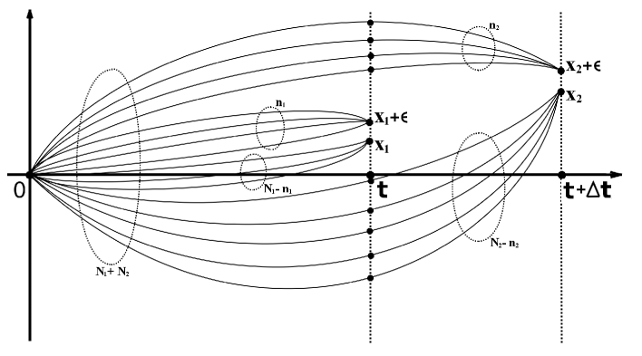
Figure 5: Schematic representation of the directed polymer paths corresponding to eq.(9.37)

Substituting the explicit expressions for the wave function (9.14) into eq.(9.37) we get:

$${\cal Z}_{\epsilon}\bigl{(}N_{1},n_{1},N_{2},n_{2},x_{1},x_{2},t,\Delta t\bigr{)}\;=\;C(N_{1}+N_{2},t)\,C(N_{2},\Delta t)\times$$

$$\times\int_{-\infty}^{+\infty}\,Dy\;\int_{-\infty}^{+\infty}\,Dz\;\exp\Biggl{\{}-\frac{\beta}{2t}\Biggl{[}(N_{1}-n_{1})x_{1}^{2}+n_{1}(x_{1}+\epsilon)^{2}+\sum_{a=1}^{N_{2}-n_{2}}y_{a}^{2}+\sum_{a=1}^{n_{2}}z_{a}^{2}\Biggr{]}\,-$$

$$\hskip 65.44133pt-\frac{\beta}{2t}A(N_{1}+N_{2},t)\Biggl{[}(N_{1}-n_{1})x_{1}+n_{1}(x_{1}+\epsilon)+\sum_{a=1}^{N_{2}-n_{2}}y_{a}+\sum_{a=1}^{n_{2}}z_{a}\Biggr{]}^{2}\,-$$

$$\hskip 65.44133pt-\frac{\beta}{2\Delta t}\Biggl{[}\sum_{a=1}^{N_{2}-n_{2}}(y_{a}-x_{2})^{2}+\sum_{a=1}^{n_{2}}(z_{a}-x_{2}-\epsilon)^{2}\Biggr{]}\,-$$

$$\hskip 65.44133pt-\frac{\beta}{2\Delta t}A(N_{2},\Delta t)\Biggl{[}\sum_{a=1}^{N_{2}-n_{2}}(y_{a}-x_{2})+\sum_{a=1}^{n_{2}}(z_{a}-x_{2}-\epsilon)\Biggr{]}^{2}\,+$$

$$\hskip 65.44133pt+\frac{\beta}{\Delta t}B(N_{2},\Delta t)\Bigl{(}\sum_{a=1}^{N_{2}-n_{2}}y_{a}+\sum_{a=1}^{n_{2}}z_{a}\Bigr{)}\Bigl{[}(N_{2}-n_{2})x_{2}+n_{2}(x_{2}+\epsilon)\Bigr{]}\Biggr{\}}$$ (9.39)

where $A(N,t)$, $B(N,t)$ and $C(N,t)$ are given in eqs.(9.15)-(9.17). Introducing $N_{2}$-component vector ${\boldsymbol{\chi}}=\{y_{1},...,y_{N_{2}-n_{2}},z_{1},...,z_{n_{2}}\}$ after simple algebra we get

$${\cal Z}_{\epsilon}\bigl{(}N_{1},n_{1},N_{2},n_{2},x_{1},x_{2},t,\Delta t\bigr{)} = C(N_{1}+N_{2},t)\,C(N_{2},\Delta t)\times$$ (9.40)

$$\times \Biggl{[}\prod_{a=1}^{N_{2}}\int_{-\infty}^{+\infty}d\chi_{a}\Biggr{]}\;\exp\Biggl{\{}-\frac{1}{2}\sum_{a,b=1}^{N_{2}}T_{ab}\chi_{a}\chi_{b}\;+\;\sum_{a=1}^{N_{2}}L_{a}\chi_{a}-\frac{1}{2}\beta G\Biggr{\}}$$

where

$$G = \frac{1}{t}\bigl{[}n_{1}(x_{1}+\epsilon)^{2}+(N_{1}-n_{1})x_{1}^{2}\bigr{]}\;+\;\frac{1}{\Delta t}\bigl{[}n_{2}(x_{2}+\epsilon)^{2}+(N_{2}-n_{2})x_{2}^{2}\bigr{]}\;+$$ (9.41)

$$+ \frac{1}{t}A(N_{1}+N_{2},t)\bigl{(}N_{1}x_{1}+n_{1}\epsilon\bigr{)}^{2}\;+\;\frac{1}{\Delta t}A(N_{2},\Delta t)\bigl{(}N_{2}x_{2}+n_{2}\epsilon\bigr{)}^{2}$$

and

$$T_{ab} = \gamma\,\delta_{ab}\;+\;\kappa$$ (9.42)

$$\gamma = \beta\frac{t+\Delta t}{t\Delta t}$$ (9.43)

$$\kappa = \frac{\beta}{t}A(N_{1}+N_{2},t)\;+\;\frac{\beta}{\Delta t}A(N_{2},\Delta t)$$ (9.44)

$$L_{a} = L\;+\;X_{a}$$ (9.45)

$$L = -\frac{\beta}{t}A(N_{1}+N_{2},t)\bigl{(}N_{1}x_{1}+n_{1}\epsilon\bigr{)}\;+\;\frac{\beta}{\Delta t}\bigl{[}A(N_{2},\Delta t)+B(N_{2},\Delta t)\bigr{]}\bigl{(}N_{2}x_{2}+n_{2}\epsilon)$$ (9.46)

$$X_{a} = \left\{\begin{array}[]{ll}x_{2}+\epsilon,&\mbox{for $a=1,...,n_{2}$}\\ x_{2},&\mbox{for $a=n_{2}+1,...,N_{2}$}\end{array}\right.$$ (9.49)

Simple integration over $\chi$’s in eq.(9.40) yields:

$${\cal Z}_{\epsilon}\bigl{(}N_{1},n_{1},N_{2},n_{2},x_{1},x_{2},t,\Delta t\bigr{)}\; = \;C(N_{1}+N_{2},t)\,C(N_{2},\Delta t)\times$$ (9.50)

$$\times \exp\Biggl{\{}-\frac{1}{2}\beta G-\frac{1}{2}\mbox{Tr}\,\ln\hat{T}\;+\;\frac{1}{2}\sum_{a,b=1}^{N_{2}}L_{a}L_{b}\hat{T}^{-1}_{ab}\Biggr{\}}$$

where

$$\mbox{Tr}\,\ln\hat{T} = N_{2}\ln\gamma\;+\;\ln\Bigl{(}1\;+\;N_{2}\frac{\kappa}{\gamma}\Bigr{)}$$ (9.51)

$$\hat{T}^{-1}_{ab} = \frac{1}{\gamma}\delta_{ab}\;-\;\frac{\kappa}{\gamma\bigl{(}\gamma+N_{2}\kappa\bigr{)}}$$ (9.52)

Simple calculations yield:

$${\cal Z}_{\epsilon}\bigl{(}N_{1},n_{1},N_{2},n_{2},x_{1},x_{2},t,\Delta t\bigr{)}\;=\;C(N_{1}+N_{2},t)\,C(N_{2},\Delta t)\;\times$$

$$\hskip 28.45274pt\times\exp\Biggl{\{}-\frac{1}{2}\beta G-\frac{1}{2}N_{2}\ln\gamma-\frac{1}{2}\ln\Bigl{(}1+N_{2}\frac{\kappa}{\gamma}\Bigr{)}-\frac{L^{2}N_{2}}{2(\gamma+N_{2}\kappa)}+\frac{\beta L}{\gamma\Delta t}\bigl{(}N_{2}x_{2}+n_{2}\epsilon\bigr{)}-$$

$$\hskip 28.45274pt-\frac{\beta\kappa N_{2}(N_{2}x_{2}+n_{2}\epsilon)}{\gamma\Delta t(\gamma+N_{2}\kappa)}-\frac{\beta^{2}\kappa(N_{2}x_{2}+n_{2}\epsilon)^{2}}{2\gamma(\Delta t)^{2}(\gamma+N_{2}\kappa)}+\frac{\beta^{2}}{2\gamma(\Delta t)^{2}}\Bigl{[}(N_{2}-n_{2})x_{2}^{2}+n_{2}(x_{2}+\epsilon)^{2}\Bigr{]}\Biggr{\}}$$ (9.53)

Next step of the calculations is to take the limits $N_{1,2}\to 0$. Using explicit expressions (9.15)-(9.17), (9.41), (9.44) and (9.46), one easily finds:

$$\lim_{N\to 0}C(N,t) = 1$$ (9.54)

$$\lim_{N\to 0}A(N,t) = -\frac{1}{3}\beta ut^{2}$$ (9.55)

$$\lim_{N\to 0}B(N,t) = \frac{1}{2}\beta ut^{2}$$ (9.56)

$$\lim_{N_{1},N_{2}\to 0}\beta G = \frac{\beta n_{1}\epsilon}{t}(2x_{1}+\epsilon)+\frac{\beta n_{2}\epsilon}{\Delta t}(2x_{2}+\epsilon)-\frac{1}{3}(\beta n_{1}\epsilon)^{2}ut-\frac{1}{3}(\beta n_{2}\epsilon)^{2}u\Delta t$$ (9.57)

$$\lim_{N_{1},N_{2}\to 0}L = \frac{1}{3}\beta^{2}n_{1}\epsilon ut+\frac{1}{6}\beta^{2}n_{2}\epsilon u\Delta t$$ (9.58)

$$\lim_{N_{1},N_{2}\to 0}\kappa = -\frac{1}{3}\beta^{2}u(t+\Delta t)$$ (9.59)

Substituting the above limiting values into eq.(9.53) we get

$$\lim_{N_{1,2}\to 0}{\cal Z}_{\epsilon}\bigl{(}N_{1},n_{1},N_{2},n_{2},x_{1},x_{2},t,\Delta t\bigr{)}\;\equiv\;Z_{\epsilon}\bigl{(}n_{1},n_{2},x_{1},x_{2},t,\Delta t\bigr{)}\;=$$

$$=\exp\Biggl{\{}-\frac{\beta n_{1}\epsilon}{2t}(2x_{1}+\epsilon)-\frac{\beta n_{2}\epsilon}{2(t+\Delta t)}(2x_{2}+\epsilon)+\frac{1}{6}(\beta n_{1}\epsilon)^{2}ut+\frac{1}{6}(\beta n_{2}\epsilon)^{2}u(t+\Delta t)+\frac{(\beta n_{1}\epsilon)(\beta n_{2}\epsilon)ut^{2}}{3(t+\Delta t)}\Biggr{\}}$$ (9.60)

Substituting the above result into eq.(9.35) and introducing notations $\beta n_{1,2}\epsilon\;=\;s_{1,2}$ in the limit $\epsilon\to 0$ we obtain:

$$\int\int_{-\infty}^{+\infty}dv_{1}dv_{2}\;P_{x_{1},x_{2}t,\Delta t}(v_{1},v_{2})\exp\bigl{\{}s_{1}v_{1}+s_{2}v_{2}\bigr{\}}\;=\;$$

$$=\exp\Biggl{\{}-\frac{x_{1}}{t}s_{1}-\frac{x_{2}}{t+\Delta t}s_{2}+\frac{1}{6}uts_{1}^{2}+\frac{1}{6}u(t+\Delta t)s_{2}^{2}+\frac{ut^{2}}{3(t+\Delta t)}s_{1}s_{2}\ \Biggr{\}}$$ (9.61)

Redefining

$$s_{1} = \sqrt{\frac{3}{ut}}\;\omega_{1}$$ (9.62)

$$s_{2} = \sqrt{\frac{3}{u(t+\Delta t)}}\;\omega_{2}$$ (9.63)

$$v_{1} = -\frac{x_{1}}{t}\;+\;\sqrt{\frac{1}{3}ut}\;\tilde{v}_{1}$$ (9.64)

$$v_{2} = -\frac{x_{2}}{t+\Delta t}\;+\;\sqrt{\frac{1}{3}u(t+\Delta t)}\;\tilde{v}_{2}$$ (9.65)

$$\Delta t = \xi\,t$$ (9.66)

we get the following relation for the probability distribution function ${\cal P}_{\xi}\bigl{(}\tilde{v}_{1},\,\tilde{v}_{2}\bigr{)}$ for the rescaled velocities $\tilde{v}_{1}$ and $\tilde{v}_{2}$, eqs.(9.64)-(9.65):

$$\int\int_{-\infty}^{+\infty}d\tilde{v}_{1}\tilde{v}_{2}{\cal P}_{\xi}\bigl{(}\tilde{v}_{1},\,\tilde{v}_{2}\bigr{)}\exp\bigl{\{}\omega_{1}\tilde{v}_{1}+\omega_{2}\tilde{v}_{2}\bigr{\}}\;=\;\exp\Bigl{\{}\frac{1}{2}\omega_{1}^{2}+\frac{1}{2}\omega_{2}^{2}+\frac{\omega_{1}\omega_{2}}{(1+\xi)^{3/2}}\Bigr{\}}$$ (9.67)

Performing simple inverse Laplace transformation

$${\cal P}_{\xi}\bigl{(}\tilde{v}_{1},\,\tilde{v}_{2}\bigr{)}\;=\;\int\int_{-i\infty}^{+i\infty}\frac{d\omega_{1}d\omega_{2}}{(2\pi i)^{2}}\;\exp\Bigl{\{}\frac{1}{2}\omega_{1}^{2}+\frac{1}{2}\omega_{2}^{2}+\frac{\omega_{1}\omega_{2}}{(1+\xi)^{3/2}}-\omega_{1}\tilde{v}_{1}-\omega_{2}\tilde{v}_{2}\Bigr{\}}$$ (9.68)

one eventually obtain the following very simple result for the two-time velocities distribution function:

$${\cal P}_{\xi}\bigl{(}\tilde{v}_{1},\,\tilde{v}_{2}\bigr{)}\;=\;\frac{1}{2\pi}\sqrt{\frac{(1+\xi)^{3}}{(1+\xi)^{3}-1}}\;\exp\Biggl{\{}-\frac{(1+\xi)^{3}}{2\bigl{[}(1+\xi)^{3}-1\bigr{]}}\Bigl{(}\tilde{v}_{1}^{2}-2\frac{\tilde{v}_{1}\tilde{v}_{2}}{(1+\xi)^{3/2}}+\tilde{v}_{2}^{2}\Bigr{)}\Biggr{\}}$$ (9.69)

where $\xi=\Delta t/t$ is the reduced separation time parameter.

One can easily check that in the limit of infinite separation time, $\xi\to\infty$, the distributions of two velocities are getting independent:

$$\lim_{\xi\to\infty}{\cal P}_{\xi}\bigl{(}\tilde{v}_{1},\,\tilde{v}_{2}\bigr{)}\;=\;\frac{1}{2\pi}\;\exp\Bigl{\{}-\frac{1}{2}\tilde{v}_{1}^{2}-\frac{1}{2}\tilde{v}_{2}^{2}\Bigr{\}}$$ (9.70)

while in the opposite limit of coinciding times, $\xi\to 0$, one finds

$${\cal P}_{0}\bigl{(}\tilde{v}_{1},\,\tilde{v}_{2}\bigr{)}\;=\;\frac{1}{\sqrt{2\pi}}\;\exp\Bigl{\{}-\frac{1}{2}\tilde{v}_{1}^{2}\Bigr{\}}\;\delta\bigl{(}\tilde{v}_{1}-\tilde{v}_{2}\bigr{)}$$ (9.71)

as it should be.

Besides, using the exact result, eq.(9.69) one can easily compute the time dependence of the two velocities correlation function:

$$\langle\tilde{v}_{1}\tilde{v}_{2}\rangle\;=\;(1+\xi)^{-3/2}$$ (9.72)

as well as the probability distribution function for the velocities difference $\tilde{v}\equiv\tilde{v}_{2}-\tilde{v}_{1}$:

$${\cal P}_{\xi}\bigl{(}\tilde{v}\bigr{)}\;=\;\frac{1}{2\pi}\sqrt{\frac{(1+\xi)^{3/2}}{4\pi\bigl{[}(1+\xi)^{3/2}-1\bigr{]}}}\;\exp\Biggl{\{}-\frac{(1+\xi)^{3/2}}{4\bigl{[}(1+\xi)^{3/2}-1\bigr{]}}\,\tilde{v}^{2}\Biggr{\}}$$ (9.73)

IX.4 Conclusions

In this Chapter we have considered the problem of velocity distribution functions in the Burgulence problem in terms of the toy Gaussian model of (1+1) directed polymers. In particular the exact result for the two-time free energy, eq.(9.31), and two-time velocity distribution functions, eq.(9.69) has been derived. Of course the considered system is too far from the realistic one. Nevertheless, it has one important advantage: being exactly solvable, some of its statistical properties are rather non-trivial. All that, in my view, makes this model to be rather useful tool for testing new ideas and various technical aspects of the calculations (like the replica technique considered in this paper). Following the proposed route, the next step would be to consider the model with finite range correlations of the random potentials (see Chapter VIII). In terms of the replica approach here one is facing the problem of $N$-particle quantum bosons with attractive finite range interactions whose solution is not known. Nevertheless even the qualitative understanding of the structure of the $N$-particle wave function of this system (which at the qualitative level might be not so much different from that of the Bethe ansatz solution for the $\delta$-correlated potentials) could hopefully be sufficient to get some understanding of the velocity statistics in the Burgulence problem.

X Joint distribution function of free energies at two different temperatures

In this Chapter we will consider one more ”direction” in the studies of directed polymers with $\delta$-correlated random potential, eqs.(1.1)-(1.2), namely, joint statistics of the free energies (or the interfaces, in the KPZ-language) at two different temperatures defined for the same quenched disorder. In other words, we are going to study the joint probability distribution function of the free energies at two (or more) different temperatures for a given realization of the disorder potential $V[\phi,\tau]$. Some years ago similar kind of problem (under the name ”temperature chaos”) has been investigated for spin glass like systems SG-T-chaos1 ; SG-T-chaos2 ; SG-T-chaos3 ; SG-T-chaos4 as well as for directed polymers on a hierarchical lattice DP-T-chaos . Here in terms of the standard replica formalism we will derive the general scaling dependence for the reduced free energy difference ${\cal F}=F(T_{1})/T_{1}-F(T_{2})/T_{2}$ on the two temperatures $T_{1}$ and $T_{2}$ (eqs.(10.33) and (10.28) In particular, it will be shown that if the two temperatures $T_{1}\,<\,T_{2}$ are close to each other, so that $(1-T_{1}/T_{2})\;\ll\;1$, the difference of the two free energies scales as $(1-T_{1}/T_{2})^{1/3}\,t^{1/3}$ ( eq.(10.40)). It will also be shown that the left tail asymptotics of this free energy difference probability distribution function coincides with corresponding tail of the TW distribution (eq.(10.35)).

For the fixed boundary conditions, $\phi(0)=\phi(t)=0$, and for a given realization of disorder the partition function of the model defined in eqs.(1.1)-(1.2) is

$$Z(\beta,t)=\int_{\phi(0)=0}^{\phi(t)=0}{\cal D}\phi(\tau)\;\mbox{\Large e}^{-\beta H[\phi;\,V]}\;=\;\exp\bigl{(}-\beta F(\beta,t)\bigr{)}$$ (10.1)

In the limit $t\to\infty$ the free energy $F(\beta,t)$ scales as

$$F(\beta,t)=f_{0}(\beta)\,t+\frac{1}{2}\,(\beta u)^{2/3}\,t^{1/3}\,f\,,$$ (10.2)

where $f_{0}(\beta)$ is the (non-random) selfaveraging free energy density, and $f$ is a random quantity described by the GUE Tracy-Widom distribution (see Chapters II-IV).

For a given realization of the disorder potential $V[\phi,\tau]$ let us consider the above system at two different temperatures $T_{1}\not=T_{2}$. More specifically, we are going to study how the the two free energies $F(\beta_{1},t)$ and $F(\beta_{2},t)$ of the same system are related to each other. In other words, we are going to study the statistical and scaling properties of the quantity

$${\cal F}(\beta_{1},\beta_{2};\,t)\;=\;\beta_{1}F(\beta_{1},t)\,-\,\beta_{2}F(\beta_{2},t)$$ (10.3)

where, in what follows it will be assumed that $\beta_{1}\,>\,\beta_{2}$ (or $T_{1}\,<\,T_{2}$). According to the definition (10.1)

$$\exp\bigl{\{}-{\cal F}(\beta_{1},\beta_{2};\,t)\bigr{\}}\;=\;Z(\beta_{1},t)\,Z^{-1}(\beta_{2},t)$$ (10.4)

Taking $N$-th power of the the both sides of the above relation and averaging over the disorder we get

$$\int d{\cal F}P_{\beta_{1},\beta_{2},t}({\cal F})\exp\bigl{\{}-N{\cal F}\bigr{\}}=\overline{Z^{N}(\beta_{1},t)Z^{-N}(\beta_{2},t)}$$ (10.5)

where $\overline{(...)}$ denotes the averaging over the random potential $V$ and $P_{\beta_{1},\beta_{2},t}({\cal F})$ is the probability distribution function of the random quantity ${\cal F}$, eq.(10.3). Introducing the replica partition function

$${\cal Z}(M,N;\,\beta_{1},\beta_{2};\,t)\;=\;\overline{Z^{N}(\beta_{1},t)\,Z^{M-N}(\beta_{2},t)}$$ (10.6)

the relation (10.5) can be formally represented as

$$\int d{\cal F}P_{\beta_{1},\beta_{2},t}({\cal F})\exp\bigl{\{}-N{\cal F}\bigr{\}}=\lim_{M\to 0}{\cal Z}(M,N;\beta_{1},\beta_{2};t)\,.$$ (10.7)

Following the standard ”logic” of the replica technique, first it will be assumed that both $M$ and $N$ are integers such that $M>N$. Next, after computing the replica partition function ${\cal Z}(M,N;\,\beta_{1},\beta_{2};\,t)$ an analytic continuation for arbitrary (complex) values of the parameters $M$ and $N$ has to be performed and the limit $M\to 0$ has to be taken. After that, the relation (10.7) can be considered as the Laplace transform of the the probability distribution function $P_{\beta_{1},\beta_{2},t}({\cal F})$ over the parameter $N$. In the case the function ${\cal Z}(0,N;\,\beta_{1},\beta_{2};\,t)$ would have ”good” analytic properties in the complex plane of the argument $N$, this relation, at least formally, allows to reconstruct by inverse Laplace transform the probability distribution function $P_{\beta_{1},\beta_{2},t}({\cal F})$. At present, for the considered problem it is possible to derive an explicit expression for the function ${\cal Z}(0,N;\,\beta_{1},\beta_{2};\,t)$ only in the limit $N\gg 1$. Nevertheless, using the relation (10.7) this allows to reconstruct the left tail (${\cal F}\to-\infty$) of the distribution function $P_{\beta_{1},\beta_{2},t}({\cal F})$. Moreover, it also allows to derive the scaling dependence of free energy difference ${\cal F}$ on $\beta_{1},\beta_{2}$ and $t$. Indeed, in the case the replica partition function has an exponential asymptotics

$${\cal Z}(0,N\to\infty;\beta_{1},\beta_{2};t\to\infty)\sim\exp\bigl{\{}A(\beta_{1},\beta_{2})tN^{\alpha}\bigr{\}},$$ (10.8)

the left tail of the probability distribution function assumes the stretched-exponential form

$$P_{\beta_{1},\beta_{2},t}({\cal F}\to-\infty)\;\sim\;\exp\bigl{\{}-B(\beta_{1},\beta_{2};\,t)\,|{\cal F}|^{\omega}\bigr{\}}\,.$$ (10.9)

Then the saddle-point estimate of the integral in the l.h.s of eq.(10.7) yields:

$$\int d{\cal F}\exp\bigl{\{}-B\,|{\cal F}|^{\omega}+N|{\cal F}|\bigr{\}}\;\sim\;\exp\bigl{\{}(\omega-1)\omega^{-\frac{\omega}{\omega-1}}B^{-\frac{1}{\omega-1}}N^{\frac{\omega}{\omega-1}}\bigr{\}}$$ (10.10)

so that

$$\exp\bigl{\{}(\omega-1)\omega^{-\frac{\omega}{\omega-1}}B^{-\frac{1}{\omega-1}}N^{\frac{\omega}{\omega-1}}\bigr{\}}\;\sim\;\exp\bigl{\{}A\,t\,N^{\alpha}\bigr{\}}$$ (10.11)

From this relation we find that

$$\omega\,=\,\alpha/(\alpha-1)$$ (10.12)

and

$$B\;=\;(\alpha-1)\,\alpha^{-\frac{\alpha}{\alpha-1}}\,\bigl{(}A\,t\bigr{)}^{-\frac{1}{\alpha-1}}$$ (10.13)

Substituting this into eq.(10.9) we get

$$P_{\beta_{1},\beta_{2},t}({\cal F}\to-\infty)\sim\exp\Bigl{\{}-(\alpha-1)\,\Biggl{(}\frac{|{\cal F|}}{\alpha\bigl{(}At\bigr{)}^{1/\alpha}}\Biggr{)}^{\frac{\alpha}{\alpha-1}}\Bigr{\}}.$$ (10.14)

If we assume that the (unknown) entire probability distribution function has a universal shape the above asymptotic behavior implies that the considered quantity ${\cal F}$ scales as follows

$${\cal F}\;=\;\bigl{(}A(\beta_{1},\beta_{2})\bigr{)}^{1/\alpha}t^{1/\alpha}\,f$$ (10.15)

where the random quantity $f\sim 1$ is described by some (unknown) probability distribution function ${\cal P}(f)$ with the left asymptotics ${\cal P}(f\to-\infty)\sim\exp\bigl{\{}-(\mbox{const})|f|^{\alpha/(\alpha-1)}\bigr{\}}$.

Thus, the above speculations demonstrates that even if we know the replica partition function only in the limit $N\gg 1$, we can still derive not only the left tail of the distribution function, but (supposing that the entire distribution function is universal) the general scaling of the free energy. Let us consider now how this replica scheme can be applied for the concrete system under consideration.

Performing the averaging over the random potential in eq.(10.6) we get

$${\cal Z}(M,N;\beta_{1},\beta_{2};t)=\prod_{a=1}^{M}\int_{\phi_{a}(0)=0}^{\phi_{a}(t)=0}{\cal D}\phi_{a}(\tau)\exp\bigl{\{}-H_{M}[\boldsymbol{\phi}]\bigr{\}}$$ (10.16)

where $H_{M}[\boldsymbol{\phi}]$ is the replica Hamiltonian

$$H_{M}[\boldsymbol{\phi}]\;=\;\int_{0}^{t}d\tau\Biggl{[}\frac{1}{2}\sum_{a=1}^{M}\beta_{a}\Bigl{(}\partial_{\tau}\phi_{a}(\tau)\Bigr{)}^{2}-\frac{1}{2}\,u^{2}\sum_{a\not b=1}^{M}\beta_{a}\beta_{b}\,\delta(\phi_{a}-\phi_{b})\Biggr{]}$$ (10.17)

with

$$\beta_{a}\;=\;\left\{\begin{array}[]{ll}\beta_{1}\,\;\;\mbox{for}\;a=1,...,N\\ \\ \beta_{2}\,\;\;\mbox{for}\;a=N+1,...,M,\end{array}\right.$$ (10.18)

Introducing:

$$\Psi(x_{1},...,x_{M};t)\;\equiv\;\prod_{a=1}^{M}\int_{\phi_{a}(0)=0}^{\phi_{a}(t)=x_{a}}{\cal D}\phi_{a}(\tau)\;\exp\bigl{\{}-H_{M}[\boldsymbol{\phi}]\bigr{\}}$$ (10.19)

one can easily show that $\Psi({\bf x};t)$ is the wave function of $M$-particle boson system with attractive $\delta$-interaction defined by the Schrödinger equation:

$$-\partial_{t}\Psi({\bf x};t)\;=\;\sum_{a=1}^{M}\frac{1}{2\beta_{a}}\partial_{x_{a}}^{2}\Psi({\bf x};t)+\frac{1}{2}u^{2}\sum_{a\not=b}^{M}\beta_{a}\beta_{b}\delta(x_{a}-x_{b})\Psi({\bf x};t)$$ (10.20)

with the initial condition $\Psi({\bf x};0)=\Pi_{a=1}^{M}\delta(x_{a})$. According to the definitions (10.16) and (10.19),

$${\cal Z}(M,N;\,\beta_{1},\beta_{2};\,t)\,=\,\Psi(x_{1},...,x_{M};t)\Big{|}_{x_{a}=0}$$ (10.21)

The time dependent wave function $\Psi({\bf x};\,t)$ of the above quantum problem can be represented in terms of the linear combination of the eigenfunctions $\Psi({\bf x})$ defined by the solutions of the eigenvalue equation

$$2E\Psi({\bf x})=\sum_{a=1}^{M}\frac{1}{\beta_{a}}\partial_{x_{a}}^{2}\Psi({\bf x})+u^{2}\sum_{a\not=b}^{M}\beta_{a}\beta_{b}\delta(x_{a}-x_{b})\Psi({\bf x})$$ (10.22)

Unlike the case with all $\beta$’s equal Lieb-Liniger ; McGuire ; Yang , for the time being, the general solution of this equation is not known. However, if we do not pretend to derive the exact result for the entire probability distribution function $P_{\beta_{1},\beta_{2},t}({\cal F})$ but we want to know only its left tail asymptotics in the limit $t\to\infty$ then it would be enough to get the behavior of the replica partition function ${\cal Z}(0,N\to\infty;\,\beta_{1},\beta_{2};\,t\to\infty)$ which is defined by the ground state solution only:

$$\Psi({\bf x};t\to\infty)\;\sim\;\exp\bigl{\{}-E_{g.s.}t\bigr{\}}\,\Psi_{g.s.}({\bf x})$$ (10.23)

One can easily check that the ground state solution of eq.(10.22) is given by the eigenfunction

$$\Psi_{g.s.}({\bf x})\;\propto\;\exp\Biggl{\{}-\frac{1}{2}\,u\sum_{a,b=1}^{M}\gamma_{ab}\,\big{|}x_{a}-x_{b}\big{|}\Biggr{\}}$$ (10.24)

where

$$\gamma_{ab}\;=\;\frac{\beta_{a}^{2}\,\beta_{b}^{2}}{\beta_{a}+\beta_{b}}$$ (10.25)

The corresponding ground state energy is

$$E_{g.s.}(M,N,\beta_{1},\beta_{2})=-\frac{1}{2}u^{2}\sum_{a=1}^{M}\frac{1}{\beta_{a}}\Biggl{(}\sum_{b=1}^{a-1}\gamma_{ab}-\sum_{b=a+1}^{M}\gamma_{ab}\Biggr{)}^{2}$$ (10.26)

Note that in the trivial case $\beta_{1}=\beta_{2}=\beta$, using eqs.(10.24)-(10.26), one easily recovers the well known ground state solution $\psi_{g.s.}\propto\exp\bigl{\{}-\frac{1}{4}\,u\beta^{3}\sum_{a,b=1}^{M}\big{|}x_{a}-x_{b}\big{|}\bigr{\}}$ and $E_{g.s.}\;=\;-\frac{1}{24}u^{2}\beta^{5}(M^{3}-M)$. Substituting eqs.(10.18) and (10.25) into eq.(10.26) after simple algebra in the limit $M\to 0$ we obtain

$$E_{g.s.}(0,N,\beta_{1},\beta_{2})=-\frac{u^{2}}{24}\lambda(\beta_{1},\beta_{2})N^{3}+\frac{u^{2}}{24}\bigl{(}\beta_{1}^{5}-\beta_{2}^{5}\bigr{)}\,N$$ (10.27)

where

$$\lambda(\beta_{1},\beta_{2}) = 4\bigl{(}\beta_{1}^{5}-\beta_{2}^{5}\bigr{)}-6\bigl{(}\beta_{1}-\beta_{2}\bigr{)}\frac{2\beta_{1}^{4}\beta_{2}+2\beta_{2}^{4}\beta_{1}+\beta_{1}^{5}+\beta_{2}^{5}}{\beta_{1}+\beta_{2}}$$ (10.28)

$$+ 3\bigl{(}\beta_{1}-\beta_{2}\bigr{)}^{2}\frac{\beta_{1}^{3}(2\beta_{2}+\beta_{1})^{2}-\beta_{2}^{3}(2\beta_{1}+\beta_{2})^{2}}{(\beta_{1}+\beta_{2})^{2}}$$

According to eqs.(10.21) and (10.23) we find

$${\cal Z}(0,N\to\infty;\beta_{1},\beta_{2};t\to\infty)\;\sim\;\exp\Bigl{\{}\frac{u^{2}}{24}\lambda(\beta_{1},\beta_{2})\,N^{3}t-\frac{u^{2}}{24}\bigl{(}\beta_{1}^{5}-\beta_{2}^{5}\bigr{)}Nt\Bigr{\}}$$ (10.29)

The second (linear on $N$ term) in the exponential of the above relation provides the contribution to the selfaveraging (non-random) linear in time part of the free energy variance ${\cal F}$. Substituting eq.(10.29) into eq.(10.7) and redefining

$${\cal F}\;=\;\frac{1}{24}u^{2}\,\bigl{(}\beta_{1}^{5}-\beta_{2}^{5}\bigr{)}\,t\;+\;\tilde{{\cal F}}$$ (10.30)

we find that in the limits $t\to\infty$ and $N\to\infty$ the left tail of the probability distribution function for the random quantity $\tilde{{\cal F}}$ (as $\tilde{{\cal F}}\to-\infty$) is defined by the relation

$$\int d\tilde{{\cal F}}\,P_{\beta_{1},\beta_{2},t}(\tilde{{\cal F}})\exp\bigl{\{}-N\tilde{{\cal F}}\bigr{\}}\sim\exp\Bigl{\{}\frac{u^{2}}{24}\,\lambda(\beta_{1},\beta_{2})N^{3}t\Bigr{\}}.$$ (10.31)

Redefining

$$N\;=\;2(u^{2}\lambda)^{-1/3}\,s$$ (10.32)

we find that the free energy difference $\tilde{{\cal F}}$ scales as

$$\tilde{{\cal F}}\;=\;\frac{1}{2}\,u^{2/3}\,\bigl{(}\lambda(\beta_{1},\beta_{2})\bigr{)}^{1/3}\,t^{1/3}\,f$$ (10.33)

where the left tail of the universal probability distribution function ${\cal P}(f)$ of the random quantity $f$ is defined by the relation

$$\int\,df\,{\cal P}(f)\,\exp\bigl{\{}-s\,f\bigr{\}}\;\sim\;\exp\Bigl{\{}\frac{1}{3}\,s^{3}\Bigr{\}}.$$ (10.34)

Simple saddle-point estimate of the above integral (for $s\gg 1$ and $|f|\gg 1$) yields

$${\cal P}(f\to-\infty)\;\sim\;\exp\Bigl{\{}-\frac{2}{3}\,|f|^{2/3}\Bigr{\}}.$$ (10.35)

Note that this tail coincides with the corresponding asymptotics of the usual free energy TW distribution TW-GUE (both GUE, GOE and GSE) but this tells nothing about its entire exact shape which at present stage remains unknown.

Let us consider in more detail the scaling relation (10.33) which demonstrate the dependence of the typical value of the fluctuating part of the reduced free energy difference, eq.(10.3), on the strength of disorder $u$, on the inverse temperatures $\beta_{1}$ and $\beta_{2}$, and on time $t$. First of all, one notes that the disorder scaling $\sim u^{2/3}$ as well as and time scaling $\sim t^{1/3}$ coincide with the ones of the usual free energy scaling in $(1+1)$ directed polymers, which of course is not surprising. On the other hand, the dependence on the inverse temperatures $\beta_{1}$ and $\beta_{2}$ turns out to be less trivial.

First of all, using explicit expression (10.28) one easily finds that in the limit $\beta_{1}\gg\beta_{2}$ (or $T_{1}\ll T_{2}$)

$$\lambda\bigl{(}\beta_{1},\beta_{2}\bigr{)}\big{|}_{\beta_{1}\gg\beta_{2}}\,\simeq\,\beta_{1}^{5}\;,$$ (10.36)

so that in this limit the scaling relation (10.33) turns into the usual one-temperature free energy scaling

$$\tilde{{\cal F}}\;\simeq\;\beta_{1}\tilde{F}_{1}\,=\,\frac{1}{2}\bigl{(}u^{2}\beta_{1}^{5}\bigr{)}^{1/3}\,t^{1/3}\,f$$ (10.37)

In other words, in this case the free energy $F_{1}$ of the polymer with the temperature $T_{1}$ is much lower than that of the polymer with the temperature $T_{2}\gg T_{1}$, and the free energy difference $\tilde{{\cal F}}$ is dominated by the free energy $F_{1}$ as it should be.

Let us consider now what happens if the two temperature parameters $\beta_{1}$ and $\beta_{2}$ are close to each other. Introducing a small (positive) parameter

$$\epsilon\;=\;\frac{\beta_{1}\,-\,\beta_{2}}{\beta_{1}}\,\ll\,1$$ (10.38)

and substituting $\beta_{2}\,=\,(1-\epsilon)\beta_{1}$ into eq.(10.28) in the leading order in $\epsilon\ll 1$ we get

$$\lambda\;\simeq\;2\beta_{1}^{5}\,\epsilon$$ (10.39)

Substituting this into eq.(10.33) we find that in this case the fluctuating part of the the corresponding free energy difference $\tilde{{\cal F}}$, eq.(10.3), scales as

$$\tilde{{\cal F}}\;\simeq\;\frac{1}{2}\bigl{(}2u^{2}\beta_{1}^{5}\bigr{)}^{1/3}\,\Biggl{(}\frac{\beta_{1}\,-\,\beta_{2}}{\beta_{1}}\Biggr{)}^{1/3}\,t^{1/3}\,f$$ (10.40)

where the random quantity $f$ is described by a universal distribution function ${\cal P}(f)$ whose left tail asymptotics is given in eq.(10.35). The above eq.(10.40) constitutes the main result of the present study and it implies ”one more 1/3” exponent in these type of systems.

XI Conclusions

In this rather technical review we considered various aspects of the methods and ideas which allows to derive various universal statistical properties of one-dimensional directed polymers in a random potential. The special emphasis was made on the detailed description of the so called replica Bethe ansatz technique which is the combination of the usual replica method (used for systems with quenched disorder) and the Bethe ansatz wave function solution for one-dimensional $N$-particle quantum boson system (which is equivalent to the replicated representation of the original directed polymer problem). In the thermodynamic limit (the limit of infinite system size) it has been demonstrated how in terms of this technique the exact results for different types of the free energy probability distribution functions can be obtained. Besides, we derive the explicit expression for the probability distribution function for the polymer’s endpoint fluctuations. In all these cases the final (universal) results are expressed in terms of the standard Fredholm determinants which deffer from each other only by the different types of kernels.

The second part of the review was devoted to the problems which are still waiting for their solutions:

$\bullet$ The zero-temperature limit for the directed polymers in a random potential with finite correlation length (Chapter VIII). Here the problem is that the exact solution of the model with $\delta$-correlated potentials (considered in Chapters IV-VII) does not reveal any finite zero-temperature limit. The physical origin of this pathology is clear: the model with $\delta$-correlated potentials is ill defined at short scales while it is the short scales which are getting the most relevant in the limit $T\to 0$. Introducing smooth finite size correlations for the random potential we can cure this pathology but in this case the solution derived for the model with $\delta$-correlated potentials becomes not valid. In Chapter VIII in terms of the standard replica technique have formulated a general scheme which hopefully would allow to obtain a finite zero-temperature limit solution for the directed polymer model with finite size correlations of the random potential.

$\bullet$ The problem of velocity distribution functions in the random force Burgers turbulence (Chapter IX). Formally, this problem is equivalent to the considered directed polymers in a random potential, but unlike the usual KPZ studies with the $\delta$-correlated random potential, in the Burgulence problem one is mainly interested in the spatial scales comparable or much smaller than the random potential correlation length . In other words, (like Chapter VIII) here one has to deal with the model with finite size correlations of the random potential whose solution is not known.

$\bullet$ Joint distribution function of the directed polymers free energies at different temperatures with the same realization of a random potential (Chapter X). Here it is possible to derive the general scaling dependence for the difference of these free energies on the two temperatures $T_{1}$ and $T_{2}$. In particular, if the two temperatures $T_{1}\,<\,T_{2}$ are close to each other, so that $(1-T_{1}/T_{2})\;\ll\;1$, the difference of the two free energies can be shown to scale as $(1-T_{1}/T_{2})^{1/3}\,t^{1/3}$. On the other hand, a general joint distribution function of these free energies remains to be computed.

Appendix A: GUE Tracy-Widom distribution function

Originally the Tracy-Widom distribution function has been derived in the context of the statistical properties of the Gaussian Unitary Ensemble (GUE) of random Hermitian matrices TW-GUE . GUE is the set of $N\times N$ random complex Hermitian matrices $G_{ij}$ (such that $G_{ij}=G_{ji}^{*}$) whose elements are drawn independently from the Gaussian distribution

$${\cal P}[{\bf G}]\;=\;B_{N}\,\exp\Bigl{\{}-\frac{1}{2}\mbox{Tr}\,\hat{G}^{2}\Bigr{\}}$$ (A.1)

where $B_{N}$ is the normalization constant. The joint probability density of $N$ eigenvalues $\{\lambda_{1},\lambda_{2},...,\lambda_{N}\}$ of such matrices has rather compact form Wigner :

$${\cal P}[\lambda_{1},\lambda_{2},...,\lambda_{N}]\;=\;C_{N}\,\prod_{i\not=j}^{N}\Big{|}\lambda_{i}-\lambda_{j}\Big{|}^{2}\exp\Bigl{\{}-\sum_{i=1}^{N}\lambda_{i}^{2}\Bigr{\}}$$ (A.2)

where $C_{N}$ is the normalization constant. Using this joint probability density one can calculate various averaged characteristics of the eigenvalue statistics. For example, one can introduce the average density of the eigenvalues $\rho(\lambda,N)\;=\;\frac{1}{N}\sum_{i=1}^{N}\langle\delta(\lambda-\lambda_{i})\rangle$ where the averaging $\langle.....\rangle$ is performed with the probability distribution, eq.(A.2). Using the symmetry of this distribution one gets

$$\rho(\lambda,N)\;=\;\prod_{i=2}^{N}\Biggl{[}\int_{-\infty}^{+\infty}\;d\lambda_{i}\Biggr{]}{\cal P}[\lambda,\lambda_{2},...,\lambda_{N}]$$ (A.3)

It can be shown Wigner that in the limit of large $N$

$$\rho(\lambda,N)\;=\;\sqrt{\frac{2}{N\pi^{2}}\;\biggl{(}1-\frac{\lambda^{2}}{2N}\biggr{)}}$$ (A.4)

We see that on average the eigenvalues lie within the finite interval $\bigl{[}-\sqrt{2N}<\lambda<\sqrt{2N}\bigr{]}$ where, according to eq.(A.4), their density has the semi-circular form. This is one of the central results of the random matrix theory which is called the Wigner semi-circular law. In particular this result tells that on average the maximum eigenvalue $\lambda_{max}$ is equal to $\sqrt{2N}$. However, at large but finite $N$ the value of $\lambda_{max}$ is the random quantity which fluctuates from sample to sample. One may ask, what is the full probability distribution of the largest eigenvalue $\lambda_{max}$? This distribution can be computed in terms of the general probability density, eq.(A.2). Introducing standard notations of the random matrix theory we define the function $F_{2}(s)\equiv\mbox{Prob}\bigl{[}\lambda_{max}<s\bigr{]}$ which gives the probability that $\lambda_{max}$ is less than a given value $s$. In these notations the functions $F_{1}(s)$, $F_{2}(s)$ and $F_{4}(s)$ denote the probability distributions of the largest eigenvalues in the Gaussian Orthogonal Ensemble (GOE), Gaussian Unitary Ensemble (GUE) and Gaussian Symplectic Ensemble (GSE) correspondingly TW2 . By definition

$$F_{2}(s)\;=\;\prod_{i=i}^{N}\Biggl{[}\int_{-\infty}^{s}\;d\lambda_{i}\Biggr{]}{\cal P}[\lambda_{1},\lambda_{2},...,\lambda_{N}]\;\equiv\;\int_{-\infty}^{s}d\lambda\,P_{TW}(\lambda)$$ (A.5)

It is this problem which has been solved by Tracy and Widom in 1994 TW-GUE . It has been shown that at large $N$ the typical fluctuations of $\lambda_{max}$ around its mean value $\sqrt{2N}$ scale as $N^{-1/6}$, namely

$$\lambda_{max}=\sqrt{2N}\;+\;\frac{1}{\sqrt{2}\,N^{1/6}}\,s$$ (A.6)

where the random quantity $s$ is described by $N$-independent distribution $P_{TW}(s)=dF_{2}(s)/ds$. The function $F_{2}(x)$, has the following explicit form

$$F_{2}(s)\;=\;\exp\biggl{(}-\int_{s}^{\infty}dt\;(t-s)\;q^{2}(t)\biggr{)}$$ (A.7)

or

$$P_{TW}(s)\;=\;\frac{d}{ds}F_{2}(s)\;=\;\exp\biggl{\{}-\int_{s}^{\infty}dt\,(t-s)q^{2}(t)\biggr{\}}\times\int_{s}^{\infty}dt\,q^{2}(t)$$ (A.8)

where the function $q(t)$ is the solution of the Panlevé II equation⁽¹⁾,

$$q^{\prime\prime}=tq+2q^{3}$$ (A.9)

with the boundary condition, $q(t\to+\infty)\sim Ai(t)$.

Figure 6: Tracy-Widom distribution function $P_{TW}(x)$, eq.(A.8).

The shape of the function $P_{TW}(s)$ is shown in Figure 6. Note that the asymptotic tails of this function are strongly asymmetric. While its right tail coincides the Airy function asymptotic $P_{TW}(s\to+\infty)\sim\exp\bigl{[}-\frac{4}{3}s^{3/2}\bigr{]}$, the left tail exhibits much faster decay $P_{TW}(s\to-\infty)\sim\exp\bigl{[}-\frac{1}{12}|s|^{3}\bigr{]}$

Appendix B: The Airy function integral relations

The Airy function $\operatorname{Ai}(x)$ is the solution of the differential equation

$$y^{\prime\prime}(x)\;=\;x\,y(x)$$ (B.1)

with the boundary condition $y(x\to+\infty)=0$. At $x\to+\infty$ this function goes to zero exponentially fast

$$\operatorname{Ai}(x\to+\infty)\;\simeq\;\frac{1}{2\sqrt{\pi}x^{1/4}}\exp\Bigl{(}-\frac{2}{3}x^{3/2}\Bigr{)}$$ (B.2)

while at $x\to-\infty$ it oscillates and decays much more slowly:

$$\operatorname{Ai}(x\to-\infty)\;\simeq\;\frac{1}{\sqrt{\pi}|x|^{1/4}}\sin\Bigl{(}\frac{2}{3}|x|^{3/2}+\frac{1}{4}\pi\Bigr{)}$$ (B.3)

The Airy function can also be represented in the integral form:

$$\operatorname{Ai}(x)\;=\;\int_{{\cal C}}\frac{dz}{2\pi i}\;\exp\Bigl{(}\frac{1}{3}z^{3}-zx\Bigr{)}$$ (B.4)

where the integration path in the complex plane starts at a point at infinity with the argument $-\pi/2<\theta_{(-)}<-\pi/3$ and ends up at a point at infinity with the argument $\pi/3<\theta_{(+)}<\pi/2$. Choosing the argument of the staring point $\theta_{(-)}=-\pi/2+\epsilon$ and that of the ending point $\theta_{(+)}=\pi/2-\epsilon$ where the positive parameter $\epsilon\to 0$ is introduced just to provide the convergence of the integration, the integration path in eq.(B.4) may coincide with the imaginary axes $z=iy$.

Below we give several useful integral relations for the Airy function which can be easily proved using the above definitions, eqs.(B.1) and (B.4) .

1. Orthogonality:

$$I_{1}\;=\;\int_{-\infty}^{+\infty}\,dx\,\operatorname{Ai}(x+u)\,\operatorname{Ai}(x+v)\;=\;\delta(u-v)$$ (B.5)

2. Just like in the well known Hubbard-Stratonovich transformation the Gaussian function is used to linearize quadratic expressions in the exponential, the Airy function can be used to linearize the cubic exponential terms:

$$I_{2}\;=\;\int_{-\infty}^{+\infty}\,dx\;\operatorname{Ai}(x)\,\exp\bigl{(}Fx\bigr{)}\;=\;\exp\Bigl{\{}\frac{1}{3}F^{3}\Bigr{\}}$$ (B.6)

where the quantity $F$ is assumed to be non negative.

3. Fourier-like integration:

$$I_{3}\;=\;\int_{-\infty}^{+\infty}\frac{dp}{2\pi}\;\operatorname{Ai}\bigl{(}ap^{2}+b\bigr{)}\;\exp\bigl{\{}ip\,c\bigr{\}}\;=\;2^{-1/3}\,a^{-1/2}\,\operatorname{Ai}\Bigl{[}2^{-2/3}(b+a^{-1/2}c)\Bigr{]}\operatorname{Ai}\Bigl{[}2^{-2/3}(b-a^{-1/2}c)\Bigr{]}$$ (B.7)

In the special case $a=1$, $\;b=u+v$ and $c=u-v$,

$$I_{3}^{\prime}\;=\;\int_{-\infty}^{+\infty}\frac{dp}{2\pi}\;\operatorname{Ai}\bigl{(}p^{2}+u+v\bigr{)}\;\exp\bigl{\{}ip\,(u-v)\bigr{]}\;=\;2^{-1/3}\operatorname{Ai}\bigl{(}2^{1/3}u\bigr{)}\operatorname{Ai}\bigl{(}2^{1/3}v\bigr{)}$$ (B.8)

4. The Airy kernel:

$$I_{4}\;=\;\int_{0}^{\infty}dx\;\operatorname{Ai}\bigl{(}x+u\bigr{)}\operatorname{Ai}\bigl{(}x+v\bigr{)}\;=\;\frac{\operatorname{Ai}\bigl{(}u\bigr{)}\operatorname{Ai}^{\prime}\bigl{(}v\bigr{)}\;-\;\operatorname{Ai}^{\prime}\bigl{(}u\bigr{)}\operatorname{Ai}\bigl{(}v\bigr{)}}{u-v}$$ (B.9)

5. The integral which transform the product of two Airy functions into one Airy function:

$$I_{5}\;=\;\int_{-\infty}^{\infty}dx\;\operatorname{Ai}(x+u)\,\operatorname{Ai}(-x/c+v)\;=\;\frac{c}{(1+c^{3})^{1/3}}\,\operatorname{Ai}\Bigl{[}\frac{u+cv}{(1+c^{3})^{1/3}}\Bigr{]}$$ (B.10)

6. Finally, the differential operator relation:

$$\exp\Bigl{\{}a\frac{\partial}{\partial x}\Bigr{\}}\,\operatorname{Ai}(x)\;=\;\operatorname{Ai}(x+a)$$ (B.11)

Appendix C: Fredholm determinant with the Airy kernel

In simplified terms the Fredholm determinant $\det\bigl{(}1-\hat{K}\bigr{)}$ can be defined as follows (for a rigorous mathematical definition see e.g. Mehta ):

$$\det\bigl{(}1-\hat{K}\bigr{)}\;=\;1\;+\;\sum_{n=1}^{\infty}\frac{(-1)^{n}}{n!}\int\int...\int_{a}^{b}dt_{1}dt_{2}...dt_{n}\;\det\Bigl{[}K(t_{i},t_{j})\Bigr{]}_{(i,j)=1,...,n}$$ (C.1)

where the kernel $\hat{K}\equiv K(t,t^{\prime})$ is a function of two variables defined in a region $a\leq(t,t^{\prime})\leq b$. Equivalently the Fredholm determinant can also be represented in the exponential form

$$\det\bigl{(}1-\hat{K}\bigr{)}\;=\;\exp\biggl{[}-\sum_{n=1}^{\infty}\frac{1}{n}\,\mbox{Tr}\,\hat{K}^{n}\biggr{]}$$ (C.2)

where

$$\mbox{Tr}\,\hat{K}^{n}\;\equiv\;\int\int...\int_{a}^{b}dt_{1}dt_{2}...dt_{n}\;K(t_{1},t_{2})K(t_{2},t_{3})...K(t_{n},t_{1})$$ (C.3)

In this Appendix following the original derivation of Tracy and Widom TW-GUE it will be demonstrated that the function $F_{2}(s)$ defined as the Fredholm determinant with the Airy kernel can be expressed in terms of the solution of the Panlevé II differential equation, namely

$$F_{2}(s)\equiv\det\bigl{[}1-\hat{K}_{A}\bigr{]}\;=\;\exp\biggl{[}-\int_{s}^{\infty}dt\,(t-s)q^{2}(t)\biggr{]}$$ (C.4)

where $\hat{K}_{A}$ is the Airy kernel defined on semi-infinite interval $[s,\infty)$:

$$K_{A}(t_{1},t_{2})\;=\;\frac{\operatorname{Ai}(t_{1})\operatorname{Ai}^{\prime}(t_{2})-\operatorname{Ai}^{\prime}(t_{1})\operatorname{Ai}(t_{2})}{t_{1}-t_{2}}$$ (C.5)

and the function $q(t)$ is the solution of the Panlevé II differential equation,

$$q^{\prime\prime}=tq+2q^{3}$$ (C.6)

with the boundary condition, $q(t\to+\infty)\sim\operatorname{Ai}(t)$.

Let us introduce a new function $R(t)$ such that

$$F_{2}(s)\;=\;\exp\biggl{[}-\int_{s}^{\infty}dtR(t)\biggr{]}$$ (C.7)

or, according to the definition, Eq.(C.4),

$$R(s)\;=\;\frac{d}{ds}\ln\Bigl{[}\det\bigl{(}1-\hat{K}_{A}\bigr{)}\Bigr{]}$$ (C.8)

Here the logarithm of the determinant can be expressed in terms of the trace:

$$\ln\Bigl{[}\det\bigl{(}1-\hat{K}_{A}\bigr{)}\Bigr{]} = -\sum_{n=1}^{\infty}\frac{1}{n}\,Tr\,\hat{K}_{A}^{n}$$

$$\equiv -\sum_{n=1}^{\infty}\frac{1}{n}\int_{s}^{\infty}dt_{1}\int_{s}^{\infty}dt_{2}\,...\,\int_{s}^{\infty}dt_{n}\;K_{A}(t_{1},t_{2})K_{A}(t_{2},t_{3})\,...\,K_{A}(t_{n},t_{1})$$

Taking derivative of this expression we gets

$$R(s) = -\int_{s}^{\infty}dt\,\bigl{(}1-\hat{K}_{A}\bigr{)}^{-1}(s,t)\,K_{A}(t,s)$$

$$\equiv -K_{A}(s,s)-\sum_{n=2}^{\infty}\int_{s}^{\infty}dt_{1}\int_{s}^{\infty}dt_{2}\,...\,\int_{s}^{\infty}dt_{n-1}\;K_{A}(s,t_{1})K_{A}(t_{1},t_{2})\,...\,K_{A}(t_{n-1},s)$$

Substituting here the integral representation of the Airy kernel, Eq.(C.5),

$$K_{A}(t_{1},t_{2})\;=\;\int_{0}^{\infty}dz\operatorname{Ai}(t_{1}+z)\,\operatorname{Ai}(t_{2}+z)$$ (C.11)

after simple algebra one gets

$$R(s)\;=\;\int_{s}^{\infty}dt_{1}\int_{s}^{\infty}dt_{2}\,\operatorname{Ai}(t_{1})\,\bigl{(}1-\hat{K}_{A}\bigr{)}^{-1}(t_{1},t_{2})\,\operatorname{Ai}(t_{2})$$ (C.12)

Taking the derivative of this expression after somewhat cumbersome algebra, we obtain

$$\frac{d}{ds}R(s)\;=\;-q^{2}(s)$$ (C.13)

where

$$q(s)\;=\;\int_{s}^{\infty}dt\,\bigl{(}1-\hat{K}_{A}\bigr{)}^{-1}(s,t)\,\operatorname{Ai}(t)$$ (C.14)

According to Eq.(C.13),

$$R(s)\;=\;\int_{s}^{\infty}dt\,q^{2}(t)$$ (C.15)

Let us introduce two more functions

$$v(s) = \int_{s}^{\infty}dt_{1}\int_{s}^{\infty}dt_{2}\,\operatorname{Ai}(t_{1})\,\bigl{(}1-\hat{K}_{A}\bigr{)}^{-1}(t_{1},t_{2})\,\operatorname{Ai}^{\prime}(t_{2})$$ (C.16)

$$p(s) = \int_{s}^{\infty}dt\,\bigl{(}1-\hat{K}_{A}\bigr{)}^{-1}(s,t)\,\operatorname{Ai}^{\prime}(t)$$ (C.17)

Taking derivatives of the above three functions $q(s)$, $v(s)$ and $p(s)$, Eqs.(C.14), (C.16) and (C.17), after somewhat painful algebra one finds the following three relations:

$$q^{\prime} = p\;-\;R\,q$$ (C.18)

$$p^{\prime} = s\,q\;-\;p\,R\;-\;2q\,v$$ (C.19)

$$v^{\prime} = -p\,q$$ (C.20)

Taking derivative of the combination $\bigl{(}R^{2}-2v\bigr{)}$ and using Eqs.(C.13) and (C.20), we get

$$\frac{d}{ds}\bigl{(}R^{2}-2v\bigr{)}\;=\;2q\,(p\;-\;R\,q)$$ (C.21)

On the other hand, multiplying Eq.(C.18) by $2q$ we find

$$\frac{d}{ds}q^{2}\;=\;2q\,(p\;-\;R\,q)$$ (C.22)

Comparing Eqs.(C.21) and (C.22) and taking into account that the value of all the above functions at $s\to\infty$ is zero, we obtain the following relation

$$R^{2}-2v\;=\;q^{2}$$ (C.23)

Finally, taking the derivative of Eq.(C.18) and using Eqs.(C.13), (C.18), (C.19) and (C.23) we easily find

$$q^{\prime\prime}\;=\;2q^{3}\;+\;sq$$ (C.24)

which is the special case of the Panlevé II differential equation Panleve ; Clarkson ; Iwasaki . Thus, substituting Eq.(C.15) into Eq.(C.7) we obtain Eq.(C.4).

In the limit $s\to\infty$ the function $q(s)$, according to its definition, eq.(C.14), must go to zero, and in this case Eq.(C.24) turns into the Airy function equation, $q^{\prime\prime}=sq$. Thus

$$q(s\to\infty)\;\simeq\;\operatorname{Ai}(s)\;\sim\;\exp\Bigl{[}-\frac{2}{3}s^{3/2}\Bigr{]}$$ (C.25)

It can be proved Hastings that in the opposite limit, $s\to-\infty$, the asymptotic form of the solution of the Panleveé equation (C.24) (which has the right tail Airy function limit, Eq.(C.25)) is

$$q(s\to-\infty)\;\simeq\;\sqrt{-\frac{1}{2}s}$$ (C.26)

The GUE Tracy-Widom probability density distribution function $P_{GUE}(t)$ is defined as

$$P_{GUE}(s)\;=\;\frac{d}{ds}\,F_{2}(s)$$ (C.27)

Substituting here Eq.(C.4), we find

$$P_{GUE}(s)\;=\;\exp\biggl{\{}-\int_{s}^{\infty}dt\,(t-s)q^{2}(t)\biggr{\}}\times\int_{s}^{\infty}dt\,q^{2}(t)$$ (C.28)

where the function $q(t)$ is the solution of the differential equation (C.24) Substituting the two asymptotics, eqs.(C.25) and (C.26), into Eq.(C.28), we can estimate the asymptotic behavior for the right and the left tails:

$$P_{GUE}(s\to+\infty) \sim \exp\Bigl{[}-\frac{4}{3}s^{3/2}\Bigr{]}$$ (C.29)

$$P_{GUE}(s\to-\infty) \sim \exp\Bigl{[}-\frac{1}{12}|s|^{3}\Bigr{]}$$ (C.30)

Appendix D: Useful combinatorial identities

In this appendix we give (without proof) several remarkable combinatorial identities.

1. Cauchy double alternant identity. In can be proved Cauchy (see also Muir ) that for a given two sets of arbitrary parameters $\{x_{1},x_{2},...,x_{N}\}$ and $\{y_{1},y_{2},...,y_{N}\}$

$$\frac{\prod_{1<a<b}^{N}\,(x_{a}-x_{b})(y_{a}-y_{b})}{\prod_{a,b=1}^{N}\,(x_{a}+x_{b})}\;=\;\det\Biggl{[}\frac{1}{x_{a}+y_{b}}\Biggr{]}_{(a,b)=1,...,N}$$ (D.1)

As a consequence, for any given set of parameters $\{Q_{1},Q_{2},...,Q_{N}\}$ and for any $x$

$$\prod_{1<a<b}^{N}\Bigg{|}\frac{Q_{a}-Q_{b}}{Q_{a}-Q_{b}+ix}\Bigg{|}^{2}\;=\;x^{N}\,\det\Biggl{[}\frac{1}{x-iQ_{a}+iQ_{b}}\Biggr{]}_{(a,b)=1,...,N}$$ (D.2)

2. For any given set of parameters $\{Q_{1},Q_{2},...,Q_{N}\}$ and for any $x$

$$\sum_{P\in S_{N}}\Biggl{\{}\prod_{1<a<b}^{N}\Biggl{[}\frac{Q_{P_{a}}-Q_{P_{b}}-x}{Q_{P_{a}}-Q_{P_{b}}}\Biggr{]}\,\frac{1}{Q_{P_{1}}\,\bigl{(}Q_{P_{1}}+Q_{P_{2}}\bigr{)}\,...\,\bigl{(}Q_{P_{1}}+...+Q_{P_{N}}\bigr{)}}\Biggr{\}}\;=\;\frac{1}{\prod_{a=1}^{N}Q_{a}}\,\prod_{1<a<b}^{N}\Biggl{[}\frac{Q_{{}_{a}}+Q_{{}_{b}}+x}{Q_{{}_{a}}+Q_{{}_{b}}}\Biggr{]}$$ (D.3)

where the summation is taken over all permutations of $N$ elements $\{Q_{1},Q_{2},...,Q_{N}\}$.

In particular, in the case $x=0$ one gets

$$\sum_{P\in S_{N}}\,\frac{1}{Q_{P_{1}}\,\bigl{(}Q_{P_{1}}+Q_{P_{2}}\bigr{)}\,...\,\bigl{(}Q_{P_{1}}+...+Q_{P_{N}}\bigr{)}}\;=\;\frac{1}{\prod_{a=1}^{N}Q_{a}}$$ (D.4)

Another version of the identity (D.3) is

$$\sum_{P\in S_{N}}\Biggl{\{}(-1)^{[P]}\frac{\prod_{1<a<b}^{N}\Bigl{(}Q_{P_{a}}-Q_{P_{b}}-x\Bigr{)}}{Q_{P_{1}}\,\bigl{(}Q_{P_{1}}+Q_{P_{2}}\bigr{)}\,...\,\bigl{(}Q_{P_{1}}+...+Q_{P_{N}}\bigr{)}}\Biggr{\}}\;=\;\frac{1}{\prod_{a=1}^{N}Q_{a}}\,\prod_{1<a<b}^{N}\Biggl{[}\frac{\bigl{(}Q_{{}_{a}}+Q_{{}_{b}}+x\bigr{)}\bigl{(}Q_{a}-Q_{b}\bigr{)}}{Q_{{}_{a}}+Q_{{}_{b}}}\Biggr{]}$$ (D.5)

where $(-1)^{[P]}$ denotes the parity of the permutation $P$.

Appendix E: Technical part of Chapter V

In this Appendix it will be shown how the factor $I_{K,L}({\bf q},{\bf n})$, eq.(5.15) can be reduced to the product of the Gamma functions. In terms of the parameters $\{m_{\alpha}\}$ and $\{s_{\alpha}\}$ the product factors in eq.(5.15) are expressed as follows:

$$\prod_{a=1}^{K}q^{(-)}_{{\cal P}_{a}^{(K)}} = \prod_{\alpha=1}^{M}\prod_{r=1}^{m_{\alpha}}{q^{\alpha}_{r}}^{(-)}$$ (E.1)

$$\prod_{a=1}^{L}q^{(+)}_{{\cal P}_{a}^{(L)}} = \prod_{\alpha=1}^{M}\prod_{r=1}^{s_{\alpha}}{{q^{*}}^{\alpha}_{r}}^{(+)}$$ (E.2)

$$\prod_{a<b}^{K}\Biggl{[}\frac{q^{(-)}_{{\cal P}_{a}^{(K)}}+q^{(-)}_{{\cal P}_{b}^{(K)}}+i\kappa}{q^{(-)}_{{\cal P}_{a}^{(K)}}+q^{(-)}_{{\cal P}_{b}^{(K)}}}\Biggr{]} = \prod_{\alpha=1}^{M}\prod_{1\leq r<r^{\prime}}^{m_{\alpha}}\Biggl{[}\frac{{q^{\alpha}_{r}}^{(-)}+{q^{\alpha}_{r^{\prime}}}^{(-)}+i\kappa}{{q^{\alpha}_{r}}^{(-)}+{q^{\alpha}_{r^{\prime}}}^{(-)}}\Biggr{]}\times\prod_{1\leq\alpha<\beta}^{M}\prod_{r=1}^{m_{\alpha}}\prod_{r^{\prime}=1}^{m_{\beta}}\Biggl{[}\frac{{q^{\alpha}_{r}}^{(-)}+{q^{\beta}_{r^{\prime}}}^{(-)}+i\kappa}{{q^{\alpha}_{r}}^{(-)}+{q^{\beta}_{r^{\prime}}}^{(-)}}\Biggr{]}$$ (E.3)

$$\prod_{c<d}^{L}\Biggl{[}\frac{q^{(+)}_{{\cal P}_{c}^{(L)}}+q^{(+)}_{{\cal P}_{d}^{(L)}}-i\kappa}{q^{(+)}_{{\cal P}_{c}^{(L)}}+q^{(+)}_{{\cal P}_{d}^{(L)}}}\Biggr{]} = \prod_{\alpha=1}^{M}\prod_{1\leq r<r^{\prime}}^{s_{\alpha}}\Biggl{[}\frac{{{q^{*}}^{\alpha}_{r}}^{(+)}+{{q^{*}}^{\alpha}_{r^{\prime}}}^{(+)}-i\kappa}{{{q^{*}}^{\alpha}_{r}}^{(+)}+{{q^{*}}^{\alpha}_{r^{\prime}}}^{(+)}}\Biggr{]}\times\prod_{1\leq\alpha<\beta}^{M}\prod_{r=1}^{s_{\alpha}}\prod_{r^{\prime}=1}^{s_{\beta}}\Biggl{[}\frac{{{q^{*}}^{\alpha}_{r}}^{(+)}+{{q^{*}}^{\beta}_{r^{\prime}}}^{(+)}-i\kappa}{{{q^{*}}^{\alpha}_{r}}^{(+)}+{{q^{*}}^{\beta}_{r^{\prime}}}^{(+)}}\Biggr{]}$$ (E.4)

$$\prod_{a=1}^{K}\prod_{c=1}^{L}\Biggl{[}\frac{q_{{\cal P}_{a}^{(K)}}-q_{{\cal P}_{c}^{(L)}}-i\kappa}{q_{{\cal P}_{a}^{(K)}}-q_{{\cal P}_{c}^{(L)}}}\Biggr{]} = \prod_{1\leq\alpha<\beta}^{M}\Biggl{\{}\prod_{r=1}^{m_{\alpha}}\prod_{r^{\prime}=1}^{s_{\beta}}\Biggl{[}\frac{q^{\alpha}_{r}-{q^{*}}^{\beta}_{r^{\prime}}-i\kappa}{q^{\alpha}_{r}+{q^{*}}^{\beta}_{r^{\prime}}}\Biggr{]}\times\prod_{r=1}^{s_{\alpha}}\prod_{r^{\prime}=1}^{m_{\beta}}\Biggl{[}\frac{{q^{*}}^{\alpha}_{r}-q^{\beta}_{r^{\prime}}-i\kappa}{{q^{*}}^{\alpha}_{r}-q^{\beta}_{r^{\prime}}}\Biggr{]}\Biggr{\}}\times$$ (E.5)

$$\times \prod_{\alpha=1}^{M}\prod_{r=1}^{m_{\alpha}}\prod_{r^{\prime}=1}^{s_{\alpha}}\Biggl{[}\frac{q^{\alpha}_{r}-{q^{*}}^{\alpha}_{r^{\prime}}-i\kappa}{q^{\alpha}_{r}-{q^{*}}^{\alpha}_{r^{\prime}}}\Biggr{]}$$

Substituting eqs.(E.1)-(E.5) into eq.(5.15), and then substituting the resulting expression into eq.(LABEL:5.22) we obtain

$$W(f) = \lim_{t\to\infty}\sum_{M=0}^{\infty}\frac{(-1)^{M}}{M!}\prod_{\alpha=1}^{M}\Biggl{[}\sum_{m_{\alpha}+s_{\alpha}\geq 1}^{\infty}\,(-1)^{m_{\alpha}+s_{\alpha}-1}\,\kappa^{m_{\alpha}+s_{\alpha}}\int_{-\infty}^{+\infty}\frac{dq_{\alpha}}{2\pi}\,{\cal G}\bigl{(}q_{\alpha},m_{\alpha},s_{\alpha}\bigr{)}$$

$$\times \exp\Bigl{\{}\lambda(t)(m_{\alpha}+s_{\alpha})\,f-\frac{t}{2\beta}\,(m_{\alpha}+s_{\alpha})q_{\alpha}^{2}\,+\,\frac{\kappa^{2}\,t}{24\beta}(m_{\alpha}+s_{\alpha})^{3}\Bigr{\}}\Biggr{]}$$

$$\times \det\Biggl{[}\frac{1}{\frac{1}{2}\kappa(m_{\alpha}+s_{\alpha})-iq_{\alpha}+\frac{1}{2}\kappa(m_{\beta}+s_{\beta})+iq_{\beta}}\Biggr{]}_{\alpha,\beta=1,...M}\times{\cal G}_{\alpha\beta}\bigl{(}{\bf q},{\bf m},{\bf s}\bigr{)}$$

where

$${\cal G}=\frac{(-1)^{s_{\alpha}}(-i\kappa)^{(m_{\alpha}+s_{\alpha})}}{\prod_{r=1}^{m_{\alpha}}{q^{\alpha}_{r}}^{(-)}\prod_{r=1}^{s_{\alpha}}{{q^{*}}^{\alpha}_{r}}^{(+)}}\prod_{r<r^{\prime}}^{m_{\alpha}}\Biggl{[}\frac{{q^{\alpha}_{r}}^{(-)}+{q^{\alpha}_{r^{\prime}}}^{(-)}+i\kappa}{{q^{\alpha}_{r}}^{(-)}+{q^{\alpha}_{r^{\prime}}}^{(-)}}\Biggr{]}\prod_{r<r^{\prime}}^{s_{\alpha}}\Biggl{[}\frac{{{q^{*}}^{\alpha}_{r}}^{(+)}+{{q^{*}}^{\alpha}_{r^{\prime}}}^{(+)}-i\kappa}{{{q^{*}}^{\alpha}_{r}}^{(+)}+{{q^{*}}^{\alpha}_{r^{\prime}}}^{(+)}}\Biggr{]}\prod_{r=1}^{m_{\alpha}}\prod_{r^{\prime}=1}^{s_{\alpha}}\Biggl{[}\frac{q^{\alpha}_{r}-{q^{*}}^{\alpha}_{r^{\prime}}-i\kappa}{q^{\alpha}_{r}-{q^{*}}^{\alpha}_{r^{\prime}}}\Biggr{]}$$ (E.7)

and

$${\cal G}_{\alpha\beta}=\prod_{r=1}^{m_{\alpha}}\prod_{r^{\prime}=1}^{m_{\beta}}\Biggl{[}\frac{{q^{\alpha}_{r}}^{(-)}+{q^{\beta}_{r^{\prime}}}^{(-)}+i\kappa}{{q^{\alpha}_{r}}^{(-)}+{q^{\beta}_{r^{\prime}}}^{(-)}}\Biggr{]}\prod_{r=1}^{s_{\alpha}}\prod_{r^{\prime}=1}^{s_{\beta}}\Biggl{[}\frac{{{q^{*}}^{\alpha}_{r}}^{(+)}+{{q^{*}}^{\beta}_{r^{\prime}}}^{(+)}-i\kappa}{{{q^{*}}^{\alpha}_{r}}^{(+)}+{{q^{*}}^{\beta}_{r^{\prime}}}^{(+)}}\Biggr{]}\prod_{r=1}^{m_{\alpha}}\prod_{r^{\prime}=1}^{s_{\beta}}\Biggl{[}\frac{q^{\alpha}_{r}-{q^{*}}^{\beta}_{r^{\prime}}-i\kappa}{q^{\alpha}_{r}+{q^{*}}^{\beta}_{r^{\prime}}}\Biggr{]}\times\prod_{r=1}^{s_{\alpha}}\prod_{r^{\prime}=1}^{m_{\beta}}\Biggl{[}\frac{{q^{*}}^{\alpha}_{r}-q^{\beta}_{r^{\prime}}-i\kappa}{{q^{*}}^{\alpha}_{r}-q^{\beta}_{r^{\prime}}}\Biggr{]}$$ (E.8)

The product factors in eq.(E.7) can be easily expressed it terms of the Gamma functions:

$$\prod_{r=1}^{m_{\alpha}}{q^{\alpha}_{r}}^{(-)} = \prod_{r=1}^{m_{\alpha}}\Bigl{[}{q_{\alpha}}^{(-)}-\frac{i\kappa}{2}(m_{\alpha}+s_{\alpha}+1)+i\kappa r\Bigr{]}\;=\;(i\kappa)^{m_{\alpha}}\frac{\Gamma\Bigl{(}\frac{1}{2}-\frac{s_{\alpha}-m_{\alpha}}{2}-\frac{i{q_{\alpha}}^{(-)}}{\kappa}\Bigr{)}}{\Gamma\Bigl{(}\frac{1}{2}-\frac{s_{\alpha}+m_{\alpha}}{2}-\frac{i{q_{\alpha}}^{(-)}}{\kappa}\Bigr{)}}$$ (E.9)

$$\prod_{r=1}^{s_{\alpha}}{{q^{*}}^{\alpha}_{r}}^{(+)} = \prod_{r=1}^{s_{\alpha}}\Bigl{[}{q_{\alpha}}^{(+)}+\frac{i\kappa}{2}(m_{\alpha}+s_{\alpha}+1)-i\kappa r\Bigr{]}\;=\;(-i\kappa)^{s_{\alpha}}\frac{\Gamma\Bigl{(}\frac{1}{2}-\frac{m_{\alpha}-s_{\alpha}}{2}+\frac{i{q_{\alpha}}^{(+)}}{\kappa}\Bigr{)}}{\Gamma\Bigl{(}\frac{1}{2}-\frac{m_{\alpha}+s_{\alpha}}{2}+\frac{i{q_{\alpha}}^{(+)}}{\kappa}\Bigr{)}}$$ (E.10)

$$\prod_{r<r^{\prime}}^{m_{\alpha}}\Biggl{[}\frac{{q^{\alpha}_{r}}^{(-)}+{q^{\alpha}_{r^{\prime}}}^{(-)}+i\kappa}{{q^{\alpha}_{r}}^{(-)}+{q^{\alpha}_{r^{\prime}}}^{(-)}}\Biggr{]} = 2^{-(m_{\alpha}-1)}\frac{\Gamma\Bigl{(}m_{\alpha}-s_{\alpha}-\frac{2i{q_{\alpha}}^{(-)}}{\kappa}\Bigr{)}\Gamma\Bigl{(}1-\frac{m_{\alpha}+s_{\alpha}}{2}-\frac{i{q_{\alpha}}^{(-)}}{\kappa}\Bigr{)}}{\Gamma\Bigl{(}\frac{m_{\alpha}-s_{\alpha}}{2}-\frac{i{q_{\alpha}}^{(-)}}{\kappa}\Bigr{)}\Gamma\Bigl{(}1-s_{\alpha}-\frac{2i{q_{\alpha}}^{(-)}}{\kappa}\Bigr{)}}$$ (E.11)

$$\prod_{r<r^{\prime}}^{s_{\alpha}}\Biggl{[}\frac{{{q^{*}}^{\alpha}_{r}}^{(+)}+{{q^{*}}^{\alpha}_{r^{\prime}}}^{(+)}-i\kappa}{{{q^{*}}^{\alpha}_{r}}^{(+)}+{{q^{*}}^{\alpha}_{r^{\prime}}}^{(+)}}\Biggr{]} = 2^{-(s_{\alpha}-1)}\frac{\Gamma\Bigl{(}s_{\alpha}-m_{\alpha}+\frac{2i{q_{\alpha}}^{(+)}}{\kappa}\Bigr{)}\Gamma\Bigl{(}1-\frac{m_{\alpha}+s_{\alpha}}{2}+\frac{i{q_{\alpha}}^{(+)}}{\kappa}\Bigr{)}}{\Gamma\Bigl{(}\frac{s_{\alpha}-m_{\alpha}}{2}+\frac{i{q_{\alpha}}^{(+)}}{\kappa}\Bigr{)}\Gamma\Bigl{(}1-m_{\alpha}+\frac{2i{q_{\alpha}}^{(+)}}{\kappa}\Bigr{)}}$$ (E.12)

$$\prod_{r=1}^{m_{\alpha}}\prod_{r^{\prime}=1}^{s_{\alpha}}\Biggl{[}\frac{q^{\alpha}_{r}-{q^{*}}^{\alpha}_{r^{\prime}}-i\kappa}{q^{\alpha}_{r}-{q^{*}}^{\alpha}_{r^{\prime}}}\Biggr{]} = \frac{\Gamma\bigl{(}1+m_{\alpha}+s_{\alpha}\bigr{)}}{\Gamma\bigl{(}1+m_{\alpha}\bigr{)}\Gamma\bigl{(}1+s_{\alpha}\bigr{)}}$$ (E.13)

Substituting the above expressions into eq.(E.7) and using the standard relations for the Gamma functions,

$$\Gamma(z)\,\Gamma(1-z) = \frac{\pi}{\sin(\pi z)}$$ (E.14)

$$\Gamma(1+z) = z\,\Gamma(z)$$ (E.15)

$$\Gamma\Bigl{(}\frac{1}{2}+z\Bigr{)} = \frac{\sqrt{\pi}\,\Gamma\bigl{(}1+2z\bigr{)}}{2^{2z}\,\Gamma\bigl{(}1+z\bigr{)}}$$ (E.16)

we get

$${\cal G}\bigl{(}q_{\alpha},m_{\alpha},s_{\alpha}\bigr{)}\;=\;\frac{\Gamma\Bigl{(}s_{\alpha}+\frac{2i}{\kappa}{q_{\alpha}}^{(-)}\Bigr{)}\,\Gamma\Bigl{(}m_{\alpha}-\frac{2i}{\kappa}{q_{\alpha}}^{(+)}\Bigr{)}\,\Gamma\bigl{(}1+m_{\alpha}+s_{\alpha}\bigr{)}}{2^{(m_{\alpha}+s_{\alpha})}\Gamma\Bigl{(}m_{\alpha}+s_{\alpha}+\frac{2i}{\kappa}{q_{\alpha}}^{(-)}\Bigr{)}\,\Gamma\Bigl{(}m_{\alpha}+s_{\alpha}-\frac{2i}{\kappa}{q_{\alpha}}^{(+)}\Bigr{)}\,\Gamma\bigl{(}1+m_{\alpha}\bigr{)}\Gamma\bigl{(}1+s_{\alpha}\bigr{)}}$$ (E.17)

Similar calculations for the factor ${\cal G}_{\alpha\beta}$, eq.(E.8), yield the following expression

$${\cal G}_{\alpha\beta}\bigl{(}{\bf q},{\bf m},{\bf s}\bigr{)} = \frac{\Gamma\Bigl{[}1+\frac{m_{\alpha}+m_{\beta}-s_{\alpha}-s_{\beta}}{2}-\frac{i}{\kappa}\bigl{(}{q_{\alpha}}^{(-)}+{q_{\beta}}^{(-)}\bigr{)}\Bigr{]}\,\Gamma\Bigl{[}1-\frac{m_{\alpha}+m_{\beta}+s_{\alpha}+s_{\beta}}{2}-\frac{i}{\kappa}\bigl{(}{q_{\alpha}}^{(-)}+{q_{\beta}}^{(-)}\bigr{)}\Bigr{]}}{\Gamma\Bigl{[}1-\frac{m_{\alpha}-m_{\beta}+s_{\alpha}+s_{\beta}}{2}-\frac{i}{\kappa}\bigl{(}{q_{\alpha}}^{(-)}+{q_{\beta}}^{(-)}\bigr{)}\Bigr{]}\,\Gamma\Bigl{[}1+\frac{m_{\alpha}-m_{\beta}-s_{\alpha}-s_{\beta}}{2}-\frac{i}{\kappa}\bigl{(}{q_{\alpha}}^{(-)}+{q_{\beta}}^{(-)}\bigr{)}\Bigr{]}}\times$$ (E.18)

$$\times \frac{\Gamma\Bigl{[}1-\frac{m_{\alpha}+m_{\beta}-s_{\alpha}-s_{\beta}}{2}+\frac{i}{\kappa}\bigl{(}{q_{\alpha}}^{(+)}+{q_{\beta}}^{(+)}\bigr{)}\Bigr{]}\,\Gamma\Bigl{[}1-\frac{m_{\alpha}+m_{\beta}+s_{\alpha}+s_{\beta}}{2}+\frac{i}{\kappa}\bigl{(}{q_{\alpha}}^{(+)}+{q_{\beta}}^{(+)}\bigr{)}\Bigr{]}}{\Gamma\Bigl{[}1-\frac{m_{\alpha}+m_{\beta}+s_{\alpha}-s_{\beta}}{2}+\frac{i}{\kappa}\bigl{(}{q_{\alpha}}^{(+)}+{q_{\beta}}^{(+)}\bigr{)}\Bigr{]}\,\Gamma\Bigl{[}1-\frac{m_{\alpha}+m_{\beta}-s_{\alpha}+s_{\beta}}{2}+\frac{i}{\kappa}\bigl{(}{q_{\alpha}}^{(+)}+{q_{\beta}}^{(+)}\bigr{)}\Bigr{]}}\times$$

$$\times \frac{\Gamma\Bigl{[}1+\frac{m_{\alpha}+m_{\beta}+s_{\alpha}+s_{\beta}}{2}+\frac{i}{\kappa}\bigl{(}q_{\alpha}-q_{\beta}\bigr{)}\Bigr{]}\,\Gamma\Bigl{[}1+\frac{-m_{\alpha}+m_{\beta}+s_{\alpha}-s_{\beta}}{2}+\frac{i}{\kappa}\bigl{(}q_{\alpha}-q_{\beta}\bigr{)}\Bigr{]}}{\Gamma\Bigl{[}1+\frac{-m_{\alpha}+m_{\beta}+s_{\alpha}+s_{\beta}}{2}+\frac{i}{\kappa}\bigl{(}q_{\alpha}-q_{\beta}\bigr{)}\Bigr{]}\,\Gamma\Bigl{[}1+\frac{m_{\alpha}+m_{\beta}+s_{\alpha}-s_{\beta}}{2}+\frac{i}{\kappa}\bigl{(}q_{\alpha}-q_{\beta}\bigr{)}\Bigr{]}}\times$$

$$\times \frac{\Gamma\Bigl{[}1+\frac{m_{\alpha}+m_{\beta}+s_{\alpha}+s_{\beta}}{2}-\frac{i}{\kappa}\bigl{(}q_{\alpha}-q_{\beta}\bigr{)}\Bigr{]}\,\Gamma\Bigl{[}1+\frac{m_{\alpha}-m_{\beta}-s_{\alpha}+s_{\beta}}{2}-\frac{i}{\kappa}\bigl{(}q_{\alpha}-q_{\beta}\bigr{)}\Bigr{]}}{\Gamma\Bigl{[}1+\frac{m_{\alpha}+m_{\beta}-s_{\alpha}+s_{\beta}}{2}-\frac{i}{\kappa}\bigl{(}q_{\alpha}-q_{\beta}\bigr{)}\Bigr{]}\,\Gamma\Bigl{[}1+\frac{m_{\alpha}-m_{\beta}+s_{\alpha}+s_{\beta}}{2}-\frac{i}{\kappa}\bigl{(}q_{\alpha}-q_{\beta}\bigr{)}\Bigr{]}}$$

References

(1) C.A. Tracy and H. Widom,
Commun. Math. Phys. 159, 151 (1994)
(2) M.Kardar, G.Parisi,Y-C.Zhang,
Phys. Rev. Lett. 56, 889 (1986)
(3) J. Baik, P.A. Deift and K. Johansson,
J. Amer. Math. Soc. 12, 1119 (1999)
(4) K. Johansson,
Comm. Math. Phys. 209, 437 (2000)
(5) M. Prähofer and H. Spohn,
Phys. Rev. Lett. 84, 4882 (2000).
(6) J. Gravner, C.A. Tracy and H. Widom,
J. Stat. Phys. 102, 1085 (2001)
(7) S.N. Majumdar and S. Nechaev,
Phys. Rev. E 69, 011103 (2004)
(8) K. Khanin, S. Nechaev, G. Oshanin, A. Sobolevski and O. Vasilyev
Phys. Rev. E 82, 061107 (2010)
(9) S.N. Majumdar and S. Nechaev,
Phys. Rev. E 72, 020901(R) (2005)
(10) P. Vivo, M.P. Pato and G. Oshanin
Phys. Rev. E 93, 052106 (2016)
(11) F. Spitzer, Adv. Math., bf 5, 246 (1970)
(12) C. Tracy and H. Widom, J. Stat. Phys., 132, 291 (2008)
(13) A. Borodin, I. Corwin and T. Sasamoto, ArXiv:1207.5035
(14) J.-I. Wakita, H. Itoh, T.Matsuyama ana M.Matsushita,
J. Phys. Soc. Jpn. 66, 67 (1997)
(15) M. Mullys, et al,
Phys. Rev. E 64, 036101 (2001)
(16) K.A. Takeuchi and M. Sano,
J. Stat. Phys., 147, 853 (2012)
(17) M.A.C. Huergo, et al,
Phys. Rev. E 85, 011918 (2012)
(18) P.J. Yunker, et al,
Phys. Rev. Lett. 110, 035501 (2013)
(19) S.Atis, et al,
Phys. Rev. Lett. 114, 234502 (2015)
(20) K.A. Takeuchi,
J. Stat. Mech.: Th. Exp. P01006 (2014)
(21) S. Lemerle, J. Ferré, C. Chappert,
V. Mathet, T. Giamarchi, and P. Le Doussal,
Phys. Rev. Lett. 80, 849 (1998).
(22) G. Blatter, M.V. Feigel’man, V.B. Geshkenbein, A.I. Larkin, and V.M. Vinokur,
Rev. Mod. Phys. 66, 1125 (1994).
(23) D. Wilkinson and J.F. Willemsen,
J. Phys. A 16, 3365 (1983).
(24) J.M. Burgers, The Nonlinear
Diffusion Equation, Reidel, Dordrecht, (1974).
(25) J. Bec and K. Khanin, Physics Reports, 447, 1 (2007)
(26) T. Halpin-Healy and Y-C. Zhang,
Phys. Rep. 254, 215 (1995).
(27) M. Kardar,
Statistical physics of fields, Cambridge: Cambridge University Press, (2007)
(28) D.A. Huse, C.L. Henley, and D.S. Fisher,
Phys. Rev. Lett. 55, 2924 (1985).
(29) D.A. Huse and C.L. Henley,
Phys. Rev. Lett. 54, 2708 (1985).
(30) M. Kardar and Y-C. Zhang,
Phys. Rev. Lett. 58, 2087 (1987).
(31) M. Kardar,
Nucl. Phys. B 290, 582 (1987).
(32) J. P. Bouchaud and H. Orland,
J. Stat. Phys. 61, 877 (1990)
(33) E. Brunet and B. Derrida,
Phys. Rev. E 61, 6789 (2000)
(34) K. Johansson,
Comm. Math. Phys. 209, 437 (2000)
(35) M. Prahofer and H. Spohn
J. Stat. Phys. 108, 1071 (2002)
(36) P. L. Ferrari and H. Spohn,
Comm. Math. Phys. 265, 1 (2006)
(37) T. Sasamoto and H. Spohn,
Phys. Rev. Lett. 104, 230602 (2010)
(38) T.Sasamoto and H.Spohn,
Nucl. Phys. B834, 523 (2010)
(39) T. Sasamoto and H. Spohn,
J. Stat. Phys. 140, 209 (2010)
(40) G. Amir, I. Corwin and J. Quastel,
Comm. Pure Appl. Math. 64, 466 (2011)
(41) V. Dotsenko,
EPL, 90,20003 (2010)
(42) P. Calabrese, P. Le Doussal and A. Rosso,
EPL, 90,20002 (2010)
(43) V. Dotsenko,
J. Stat. Mech. P07010 (2010)
(44) I. Corwin,
Random Matrices: Theory Appl. 1, 1130001 (2012)
(45) A. Borodin, I. Corwin and P. Ferrari,
Comm. Pure Appl. Math. 67, 1129–1214 (2014)
(46) P. Calabrese and P. Le Doussal,
Phys. Rev. Lett. 106, 250603 (2011)
(47) V. Dotsenko,
J. Stat. Mech. P11014 (2012)
(48) T.Gueudré and P. Le Doussal,
EPL, 100, 26006 (2012)
(49) S. Prolhac and H. Spohn,
J. Stat. Mech. P01031 (2011)
(50) V. Dotsenko,
J. Phys. A: Math. Theor. 46, 355001 (2013)
(51) T. Imamura, T. Sasamoto and H. Spohn,
J. Phys. A: Math. Theor. bf 46, 355002 (2013)
(52) S. Prolhac and H. Spohn,
J. Stat. Mech. P03020 (2011)
(53) V. Dotsenko,
Cond. Mat. Phys. 17, 33003 (2014)
(54) G.M. Flores, J. Quastel and D. Remenik,
Comm. Math. Phys. Online First Articles, November 2012
(55) G. Schehr,
J. Stat. Phys. 149(3), 385 (2012)
(56) J. Baik, K. Liechty and G. Schehr,
J. Math. Phys. 53, 083303 (2012)
(57) V. Dotsenko,
J. Stat. Mech. P02012 (2012)
(58) T. Bothner and K. Liechty,
arXiv:1212.3816v2
(59) V. Dotsenko,
J. Stat. Mech. P06017 (2013)
(60) V. Dotsenko,
J. Phys. A: Math. Theor. 48 495001 (2015)
(61) K. Johansson,
arXiv:1502.00941 (2015)
(62) P.L. Ferrari and H. Spohn,
SIGMA 12, 074 (2016)
(63) K.A. Takeuchi and M. Sano,
J. Stat. Phys. 147, 853-890 (2012)
(64) V. Dotsenko,
J. Phys. A: Math. Theor. 49 27LT01 (2016)
(65) J. De Nardis, P. Le Doussal and K.A. Takeushi,
arXiv:1611.04756v1 (2016)
(66) J. De Nardis, P. Le Doussal,
arXiv:1612.08695 (2016)
(67) P.G. De Gennes,
Phys. Lett. 38A, 339 (1972)
(68) S.F. Edwards and P.W. Anderson,
J. Phys. F 5, 965 (1975)
(69) M. Mezard, G. Parisi and M.A. Virasoro,
Spin Glass Theory and Beyond, World Scientific, Singapore (1987)
(70) Victor Dotsenko,
Introduction to the Replica Theory of Disordered statistical Systems,
Cambridge University Press, (2001)
(71) J.J.M. Verbaarschot and M.R. Zirnbauer,
J. Phys A: Math. Gen. 17, 1093 (1985)