Model-independent search for neutrino sources
with the ANTARES neutrino telescope

Abstract

A novel method to analyse the spatial distribution of neutrino candidates recorded with the ANTARES neutrino telescope is introduced, searching for an excess of neutrinos in a region of arbitrary size and shape from any direction in the sky. Techniques originating from the domains of machine learning, pattern recognition and image processing are used to purify the sample of neutrino candidates and for the analysis of the obtained skymap. In contrast to a dedicated search for a specific neutrino emission model, this approach is sensitive to a wide range of possible morphologies of potential sources of high-energy neutrino emission. The application of these methods to ANTARES data yields a large-scale excess with a post-trial significance of 2.5$\sigma$. Applied to public data from IceCube in its IC40 configuration, an excess consistent with the results from ANTARES is observed with a post-trial significance of 2.1$\sigma$.

1 Introduction

Since the recent discovery of a diffuse high-energy astrophysical neutrino flux by the IceCube Collaboration [1, 2, 3], neutrino astronomy has established itself as a new discipline. Due to the statistical limitations implied by a new observational tool that has just overcome its initial detection threshold, the spectral and spatial properties of the discovered flux are still not well constrained.

The high-energy starting event (HESE) analysis [2], which is most sensitive to the Southern sky but has a poor spatial resolution, measures a best-fit diffuse signal of $dN_{\nu}/dE\propto E^{\Gamma}$ with $\Gamma=-2.5$ [4]. The flux observed from the Northern Sky with a higher energy threshold of about 200 TeV in the muon channel exhibits a harder spectral index of about $\Gamma=-2.13\pm 0.13$ [5].

A first analysis has shown that the spatial distribution of HESE events is consistent with an isotropic distribution [6].

While there seems to be some evidence for an excess at low galactic latitudes [7], favouring a galactic contribution with a softer spectrum and an extragalactic contribution with a harder spectrum [8], the origin of the various contributions remains open.

Several analyses with the goal to reveal the origin of the astrophysical neutrinos have been performed. Time-integrated searches for point-like and extended bright sources by ANTARES [9], IceCube [10] as well as a joint search [11] exclude the possibility that the flux can be generated by a small number of bright sources. A first search employing a two-point correlation function with data from the ANTARES neutrino telescope [12] has neither found significant deviations from isotropy in the full-sky neutrino distribution nor shown evidence for correlations with catalogues of various astrophysical objects. Likewise a two-point correlation and multipole analysis of IceCube skymaps confirmed that the assumption of a small number of bright sources is excluded [13]. Therefore, a distribution of many faint point-like or unexpected extended sources constitutes a promising hypothesis at this stage.

ANTARES [14] is the largest operational neutrino telescope in the Northern Hemisphere, located in the Mediterranean Sea (42^∘48’N, 6^∘10’E) at a depth of 2475 m. Due to its location, it mainly observes the Southern sky in the upgoing muon channel and provides an excellent view of the Galactic Centre. Despite its much smaller instrumented volume compared to IceCube, it has an effective area for muon neutrinos which is comparable to that of the IceCube HESE analysis for energies around 100 TeV and even surpasses it for energies below about 60 TeV [15].

This paper introduces three independent new methods and the results obtained with them. The first two algorithms enhance the data selection and reconstruction process, while the third is a novel analysis method, referred to as multiscale method in the following, that uses the arrival directions of upgoing muon neutrinos recorded with the ANTARES neutrino telescope in 6 years of data taking.

The goal of this analysis is to identify the most significant, spatially confined excess over the background of atmospheric neutrinos without relying on assumptions of any emission model of potential neutrino sources. The analysis method is sensitive to a clustering of events in an extended sky region, and its sensitivity increases with the size of the signal region. The multiscale method does not rely on any property derived from modelling or simulations, but computes all required estimates from the observed data. Compared to other searches for potential extended sources, it has the benefit of not being restricted to a given template. In contrast to other model-independent searches, like e.g. a two-point correlation analysis, it identifies the region of a dense clustering. The method is designed to yield a first indication of a candidate source region significantly deviating from the expected background distribution, but not to provide a detection with maximum significance or to interpret the nature of a candidate cluster.

2 Data selection and reconstruction

2.1 Signal identification

In order to distinguish events resulting from genuine neutrinos from the background of atmospheric muons that reach the telescope from above and generate about $10^{6}$ times more events, cuts are placed on the direction reconstruction to select those that are consistent with an “upgoing” particle entering the telescope from below.

In this analysis a multivariate classification technique called “Random Decision Forest” (RDF) [17] is used in addition to cuts on the reconstruction quality to allow for less strict cuts, increasing the available statistics. The RDF operates on variables describing the topology and timing pattern of the light observed within ANTARES [18]. The output of this algorithm for a recorded event is an assignment to a predefined class. In this application the classes are “upgoing” and “downgoing”. The algorithm is trained on Monte Carlo simulations that incorporate the observed time-dependent data-taking conditions [19]. To improve the accuracy of the results, a two-step classification is used, where the first classification rejects only clearly downgoing signatures, while the second step is trained specifically to filter out those atmospheric muon events that generate patterns similar to the desired upgoing muon neutrinos. This technique reaches a rejection rate of $99.85\%\pm 0.12\%$ for downgoing atmospheric muons while preserving $81.7\%\pm 1.3\%$ of all charged current muon neutrino events (all numbers with respect to all triggered events, calculated for a spectrum following $E^{-2.0}$). Compared to a single stage RDF classification with a similar efficiency for upgoing neutrino events it reduces atmospheric muons by a factor of 20. Figure 1 shows the efficiency for upgoing muon neutrinos as a function of the neutrino energy. The classification accuracy is defined as $\frac{\textrm{Number of correctly classified events}}{\textrm{Total number of events}}$.

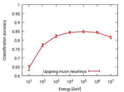
Figure 1: The classification accuracy of the two step RDF classification for upgoing muon neutrinos versus neutrino energy for Monte Carlo simulations. The error bars indicate one standard deviation of statistical errors plus an estimate of the systematic error resulting from fluctuations in the training sample.

2.2 Direction reconstruction

A novel method called “Selectfit” is used to reconstruct the direction of neutrino candidates. Instead of applying one reconstruction algorithm for all neutrino candidates, Selectfit combines the results of multiple direction reconstruction algorithms, aiming to select the most precise result for each event. It combines four reconstruction algorithms previously used by ANTARES [20, 21, 22]. While the reconstruction schemes of the algorithms that are combined are similar, each algorithm performs best for a different energy range or has different prerequisites for a successful reconstruction, allowing Selectfit to improve the overall result. The selection is again performed by a Random Decision Forest using the reconstruction results (zenith and azimuth angle) as well as all available quality-related output parameters of the considered reconstruction algorithms as input variables. It tries to identify the most accurate reconstruction result. The output class number hence determines which algorithm is used for an event.

In order to estimate the accuracy of the reconstruction for each event in a comparable way, Selectfit cannot just rely on the quality variable of the chosen algorithm. Instead it combines the results and quality parameters of all considered algorithms using a RDF. The output of this second RDF are classes corresponding to bins of angular error ( $<0.1^{\circ}$, $<0.2^{\circ}$, $<0.4^{\circ}$, $<0.8^{\circ}$, …).

As illustrated in Figure 2, Selectfit either allows the angular error for a sample of neutrinos to be reduced or it can be used to increase the sample size for a given angular error. It increases the available statistics by at least 11% for any given accuracy.

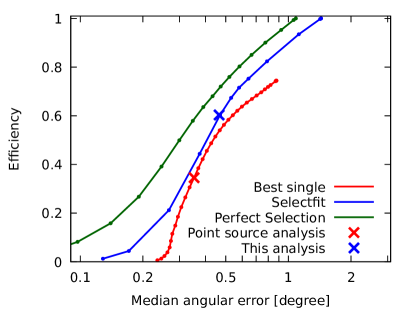
Figure 2: Comparison of the efficiency versus the median angular error of direction reconstruction algorithms. Every point of these curves is obtained for a different cut on the quality variables. Shown are the performance of the on average most accurate individual direction reconstruction algorithm [20] in red for cuts on its standard quality parameter and the novel method ”Selectfit“ with cuts on the estimated error class in blue. The crosses indicate the cuts used for the single algorithm in [23] and for Selectfit in this analysis. The green line shows the unreachable limit for the perfect combination of direction reconstruction algorithms. It is the performance if for every event the best available single reconstruction was chosen and the true angular uncertainty was used for the selection. All performances have been evaluated for a neutrino flux following an $E^{-2}$ energy spectrum. Efficiency is defined with respect to all triggered events where at least one direction reconstruction succeeded.

The benefit for small angular errors is mainly due to the improved estimation of the angular error, whereas for less accurate reconstructions, the main benefit results from the event-wise selection from the four reconstruction methods [18].

Since a search for extended sources does not necessarily require the same angular precision as a point source search, a looser cut on the uncertainty of the reconstruction is applied. For a flux of muon neutrinos with an energy spectrum of $E^{-2}$ these cuts result in a median angular uncertainty of 0.46^∘. The cut for this analysis was chosen to yield a high statistics sample of muon neutrino candidates while reconstructing them accurately enough to match the 0.5^∘ grid spacing used in the multiscale method discussed in the following section. In Figure 3 the effective area reached with this method is compared to the effective area obtained with the default reconstruction scheme as used for point-source searches [23]. The looser event selection in this analysis also results in a higher background from misreconstructed atmospheric muons in the final sample of neutrino candidates (29.7% instead of 10% in [9]).

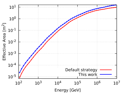
Figure 3: Comparison of the effective area for the default event selection and reconstruction strategy for point sources [23] in red and this work in blue. The ratio is about 2.5 at 100 GeV and decreases to about 1.5 for energies above 100 TeV.

3 Model-independent multiscale source search

The model-independent multiscale source search aims to identify the region of arbitrary position, size, shape and and distribution of neutrino events within the region with the most significant excess of neutrino events in the sky with respect to the background expectation.

The method itself is independent from the ANTARES neutrino telescope or the fact that the analysed data are neutrino candidates. The only assumption made in this method is that the density of background events at any declination is approximately independent of the right ascension. Unlike many techniques known from image processing, it is designed to operate also on the sparse dataset of neutrinos. While many other fields of astronomy can operate on image-like measurements, these neutrino data would fill only very few grid points of a skymap. Hence many methods successfully used in other experiments are not applicable here.

The search method consists of eight subsequent steps applied to the measured neutrino sky map, described in subsections 3.1–3.8. These steps have been defined such that they are independent from assumptions on signal topology or spectrum. They implement measures to suppress background and reduce fluctuations, to identify regions that stick out from the background, and to determine topology and significance of a possible signal. They are the result of an extensive investigation and optimisation of different methods and options, as described in [18]. Since the resulting algorithm is highly complex and not targeted at a specific signal configuration, however, it is impossible to explore whether it is optimal in the full phase space of all possible analysis methods.

Compared to the standard ANTARES point-source searches [23], the multiscale method has been estimated to require a typically 20–100% higher neutrino flux in order to make an equally significant discovery for a point source, depending on the assumed source spectrum. However, these previous searches all target specific hypotheses of neutrino production and are not designed to detect unexpected sources or distributions of sources.

3.1 The search grid

In the first step a spherical grid is defined that allows for describing the sky map in terms of sets of integers assigned to the grid points (see subsequent steps). The distance of adjacent grid points is chosen to be $0.5^{\circ}$, commensurate with the angular resolution of reconstructed neutrino-induced muon tracks in ANTARES (see Fig. 2). The grid consists of 165016 grid points. Figures 4, 5 and 6 show the spherical grid, with grid points in blue and 12000 randomly generated neutrino events in white. This number of neutrinos is close to the expectation for the data analysis and they are distributed according to the visibility of ANTARES. In order to better illustrate the steps of the analysis method, two artificial point sources with 12 and 18 events, respectively, have been added at a declination of $-70^{\circ}$, see Figures 6 and 7.

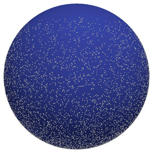
Figure 4: A spherical grid in equatorial coordinates (in blue) with 12000 randomly generated events and two point-like sources (in white). The grid points are rendered with a radius of about $0.5^{\circ}$, hence they overlap and form a closed sphere. Only the hemisphere of the three dimensional sphere facing the observer is visible in this near-side general perspective projection. View on the equator (declination of $0^{\circ}$).

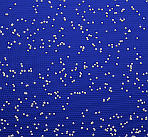
Figure 5: A zoom to the centre of Figure 4 where the grid points become visible.

Figure 6: The same setup as in Figure 4, view from below on the south pole (declination of $-90^{\circ}$). This setup contains the artificially added events as shown more clearly in Figure 7. All following spheres are oriented as in this Figure.

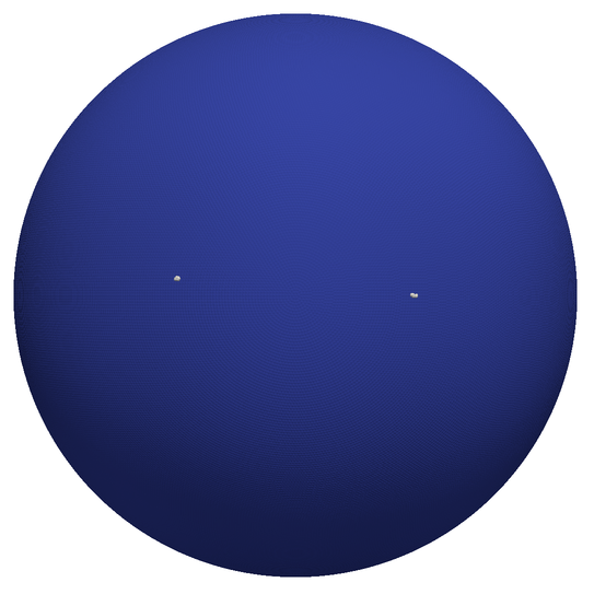
Figure 7: The same setup and orientation as Figure 6, but displayed without the random events. The remaining white points are the events of the two added point sources.

3.2 Counting

In this step, a set of integers is determined for each grid point by counting the neutrino events located in rings of different radii around that point; these integers will be analysed in the following using Poissonian statistics. The inner ring radius is referred to as the search scale, while the outer radius is $0.5^{\circ}$ larger. The search evaluates 180 scales, i.e. 180 different regions with increasing angular radius from 0^∘ up to 90^∘ in steps of 0.5^∘. This choice yields sensitivity to source regions up to an extension of twice the maximal search scale, i.e. $180^{\circ}$. The counting is performed for each grid point and for each search scale. The results are stored on an independent spherical grid for each search scale. A visualisation of the counting scheme is depicted in Figure 8. For three scales the results for the example from Figure 6 are shown in Figure 9. Note that, unless stated otherwise, in these and all following similar figures, the colour code is readjusted between the different scales to match the full range of values present on each sphere.

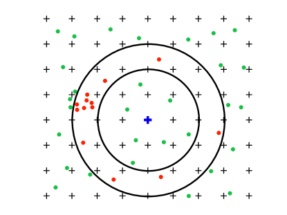
Figure 8: Scheme of the neutrino counting. Crosses mark the grid points with a distance of 0.5^∘ between them. Green and red dots correspond to neutrinos. The blue cross is the grid point that is being evaluated. The search scale (here 1.0^∘ to 1.5^∘) is defined by the black circles. Neutrinos which are counted with the current search scale around the search point are shown in red. The results of the evaluation of this scale at the blue grid point is 13.

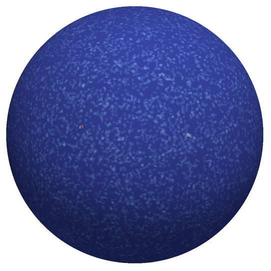
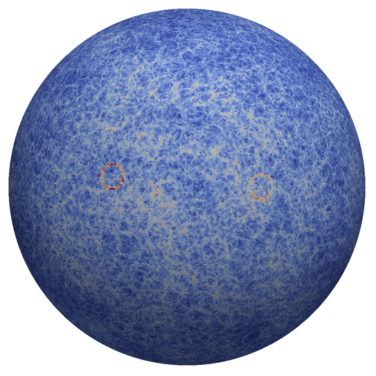
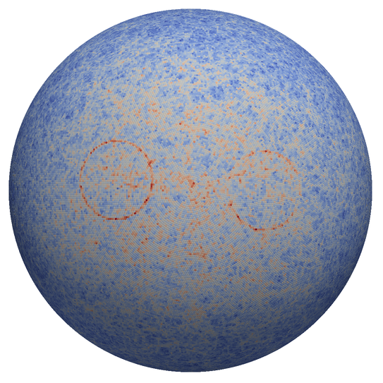
Figure 9: The spherical search grid after counting the events presented in Fig. 6 in rings between 0^∘ and 0.5^∘ (top), between 3^∘ and 3.5^∘ (middle and between 10^∘ and 10.5^∘ (bottom) around each grid point. The colour code is readjusted from top to bottom to the range of values present on each sphere.

3.3 Poisson probabilities

Poissonian probabilities $P(N,\lambda)$ are now used to infer a measure for the probability that the event numbers $N$ from the previous step exceed the background expectation. The expected mean number $\lambda$ for each grid point is estimated by pseudo-experiments using scrambled events. The scrambling is achieved by randomly shuffling the event times before converting from local to equatorial coordinates. This results in randomised distributions that preserve the characteristics of the actual data taking, for instance the distribution of the declinations or the efficiency of the data taking versus time. From the $P(N,\lambda)$, the parameter

$$Q=\log_{10}\left(\frac{1}{P(x\geq N,\lambda)}\right)=-\log_{10}(P(x\geq N,\lambda))$$ (1)

is calculated. Subsequently, a low-pass filter is applied to the $Q$ values on the spheres to reduce the influence of statistical fluctuations. These smoothed $Q$ values are called $R$ and serve as input for the next step. The search spheres after these computations are shown in Figure 10.

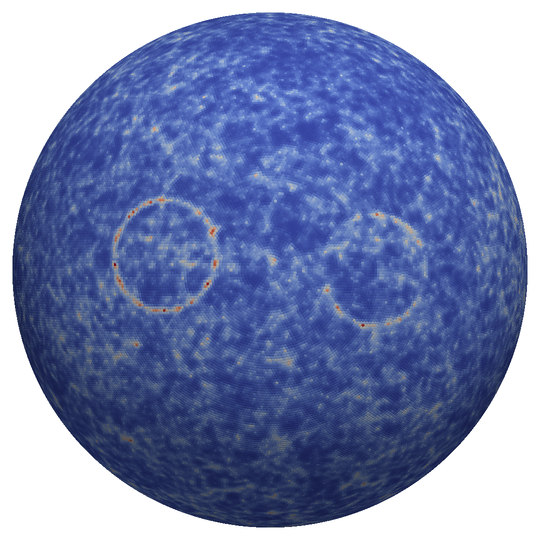
Figure 10: Colour coded $R$ values as defined in Section 3.3 derived from the event counts shown in Fig. 9 for the scales 0^∘ to 0.5^∘ (top), 3^∘ to 3.5^∘ (middle), and 10^∘ to 10.5^∘ (bottom).

3.4 Segmentation I

The next step aims to focus on potentially relevant information and to remove background fluctuations. In general, this task, well known in the field of computer vision, is called segmentation. Here it is performed using a simple threshold $\theta$. Values below the threshold, e.g. less pronounced fluctuations, are set to zero. The threshold $\theta$ is derived and applied for each search scale independently, based on the histogram of the $R$ values calculated for this scale. Figure 11 illustrates the details how the threshold is obtained. While multiple other options to determine a threshold from the histogram would be possible, no method could be identified to be significantly better than the others.

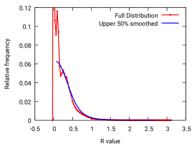
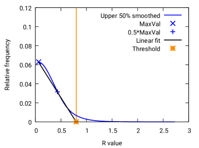
Figure 11: Left: The red histogram shows the distribution of $R$ values for one scale (0^∘ to 0.5^∘ in this example). Starting from the median value, the histogram is smoothed by Gaussian smearing to obtain the blue curve. Right: From the blue curve in the left panel the threshold $\theta$ is determined by the zero-crossing of the line through the point with the maximum y-value on the blue curve and the point with half this y-value.

The outcome of this step at a grid point $p$ is given by:

$$S_{p}=\left\{\begin{array}[]{ll}R_{p},&R_{p}\geq\theta\\ 0,&R_{p}<\theta\end{array}\right.$$ (2)

The resulting $S$ maps after the segmentations are shown in Figure 12.

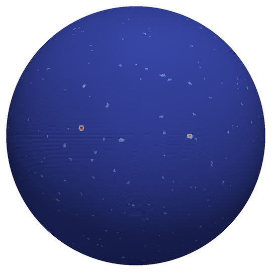
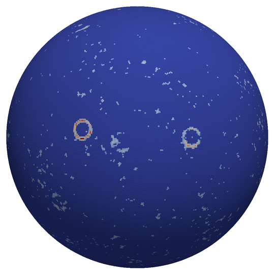
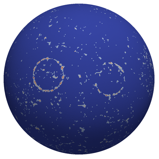
Figure 12: $S$ maps after applying the segmentation step to the data shown in Fig. 10 according to Equation 2 for the scales 0^∘ to 0.5^∘ (top), 3^∘ to 3.5^∘ (middle), and 10^∘ to 10.5^∘ (bottom).

3.5 Remapping

The $S$ maps clearly show indications of the signal, but in a re-localised way – for example, point sources are mapped to circles with the radius corresponding to the search scale. The next step is to reconstruct the original location of the neutrinos that caused the remaining high values of $S$ on the spheres. Since the values for a given search scale $d$ originate from neutrinos that are between $d$ and $d+0.5^{\circ}$ away from the grid points where the values are stored, the following approach is used: let $\text{Set}_{p}$ be the set of $N_{p}$ grid points with a distance between $d$ and $d+0.5^{\circ}$ around a grid point $p$ and let $q$ be an element (a grid point) of this set. The value $T_{p}$ for grid point $p$ is calculated by averaging over the values $S_{q}$ of all grid points in $\text{Set}_{p}$:

$$T_{p}=\sum_{q\in\text{Set}_{p}}\frac{S_{q}}{N_{q}}\,.$$ (3)

This step maps the information back to all potential origins, meaning all grid points where the neutrinos contributing to the value could have been located. Results of these computations are shown in Figure 13. A higher density in the original neutrino distribution is now encoded in the overlapping pattern of the remapped circles as seen in the middle and bottom pictures of Figure 13. Note that the halos around the original source positions are unavoidable artifacts of this method, which reduce its sensitivity for point-source searches but less so for extended sources.

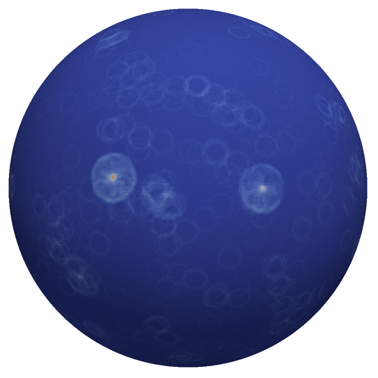
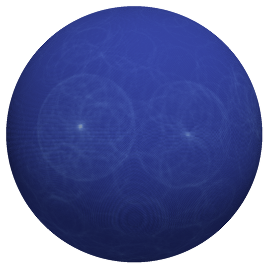
Figure 13: Values of $T$ after the remapping step applied to the data shown in Fig. 10 according to Equation 3, for the scales 0^∘ to 0.5^∘ (top) 3^∘ to 3.5^∘ (middle), and 10^∘ to 10.5^∘ (bottom). Note that the colour code is the same for all three pictures.

3.6 Summation

So far, all calculations have been made independently for each search scale. In order to derive information on size and topology of potential signal regions without imposing a distance or size scale, the results for the different search scales need to be combined. Having evaluated multiple approaches to exploit the information available in the multitude of scales, a simple sum of the maps assigned to all scales of a given spherical grid was found to yield the most robust evaluation. Since the influence of random fluctuations is high for the smallest scale, it is not included in this sum. The input for the final steps is calculated as:

$$U_{p}=\sum_{i=2}^{180}T_{p,i}\,,$$ (4)

where the index $i$ denotes the distance scale, given by $d=(i-1)\cdot 0.5^{\circ}$. This index has been omitted in the previous equations as all computations have been restricted to the same distance scale. The result of the summation according to Equation 4, applied to the full data set and all scales, can be seen in Figure 14.

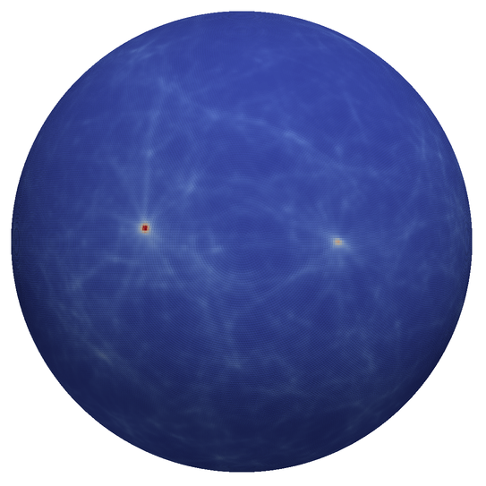
Figure 14: Values of $U$, given by Equation 4.

3.7 Segmentation II

A further segmentation is performed to isolate potential signal regions from background fluctuations. The same procedure which was used before for the histograms of $R$ values (see Section 3.4) is used here for the single histogram of $U$ values. In this step, however, different thresholds $\theta_{\beta}$ are used, obtained by scaling the difference between the minimum non-zero value found on the sphere, $U_{\mathrm{min}}$, and $\theta$, the threshold computed as in the previous segmentations, by a factor $\beta\in\mathbb{R}$:

$$\theta_{\beta}=U_{\mathrm{min}}+\beta(\theta-U_{\mathrm{min}})\,.$$ (5)

The variable threshold $\theta_{\beta}$ serves to adjust the sensitivity of the segmentation step. The result of the segmentation using $\beta$ for each grid point $p$ is given by:

$$V_{p}=\left\{\begin{array}[]{ll}U_{p},&U_{p}\geq\theta_{\beta}\\ 0,&U_{p}<\theta_{\beta}\end{array}\right.$$ (6)

Lower values for $\beta$ result in lower thresholds $\theta_{\beta}$, allowing more extended structures to be found, while higher values only preserve the high peaks, favouring smaller morphologies. The results are finally filtered using a two-dimensional median filter to suppress potential artefacts (e.g. single grid points). The effect of different thresholds for the segmentation can be seen in Figure 15. Choosing the value of $\beta$ is the first step in this analysis where an explicit bias for any source property is included. Based on an evaluation of a variety of simulated sources, two values are used: $\beta=0.75$ and $\beta=1.11$. These values are chosen to be more sensitive to extended than to small (or point-like) structures. This choice is motivated by the objective to perform a search that complements the previous, location-independent ANTARES searches for point-like sources [23].

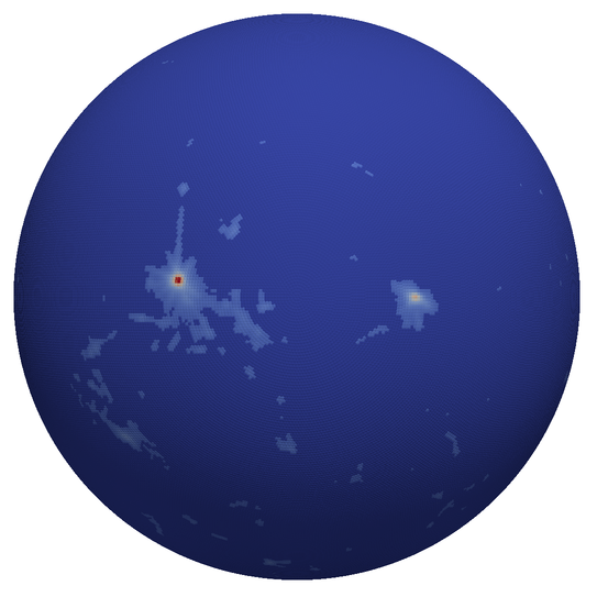
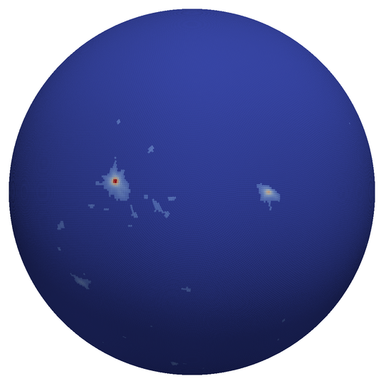
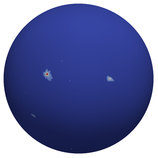
Figure 15: $V$ values after the segmentation as given by Equation 6 for $\beta=0.75$ (top), $\beta=0.95$ (middle), and $\beta=1.11$ (bottom).

3.8 Significance

A possible signal of the analysis will manifest itself as a connected group of grid points, all with values above $\theta_{\beta}$; such an object is called a “cluster”.

The final step is to distinguish potentially significant clusters from random accumulations. Since the exact size, shape, position and composition of a cluster is highly unlikely to be reproduced using pseudo-experiments, more generic metrics must be used to evaluate the significance of a cluster. Many metrics have been designed and tested on a multitude of simulated sources [18], each with different sensitivities to different sources. No single metric can be maximally sensitive to all potential sources. Motivated by the focus on extended sources, the metric “clustersize”, given by the number $N_{c}$ of grid points in a cluster, has been chosen, performing best for extended source topologies. The quantity $N_{c}$ is mainly correlated wit the size of the signal region. Some information on the density of neutrinos within a cluster is nevertheless retained, because the average value of $U$ in a given cluster, and hence the cluster size, grows with the neutrino density.

The significance for a cluster is derived from pseudo-experiments with scrambled events as explained in Section 3.3. For each threshold $\theta_{\beta}$ the distribution obtained from the pseudo-experiments has to be treated independently, as e.g. the distribution of the sizes of clusters depends on the used threshold. A pre-trial p-value and hence a pre-trial significance is computed for each observed cluster using the corresponding distribution. The distribution of the values obtained for the metric “clustersize” (in grid points) for a threshold using $\beta=0.75$ is shown in Figure 16. An exponential function $a\cdot e^{bx}$ with free parameters $a$ and $b$ is fitted to the tail of the distribution. This function is used instead of the histogram if the significance determination would be limited by the available statistics. For each pseudo-experiment, only the highest pre-trial significance of any cluster from any threshold is considered the result of this pseudo-experiment. The post-trial significance is then obtained by a comparison of the measured pre-trial significance of an observed cluster with the distribution obtained from pseudo-experiments.

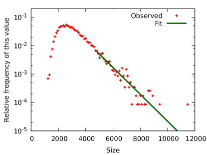
Figure 16: The distribution of the sizes of clusters from pseudo-experiments and a fit to the tail of the distribution.

3.9 Application to extended sources and general considerations

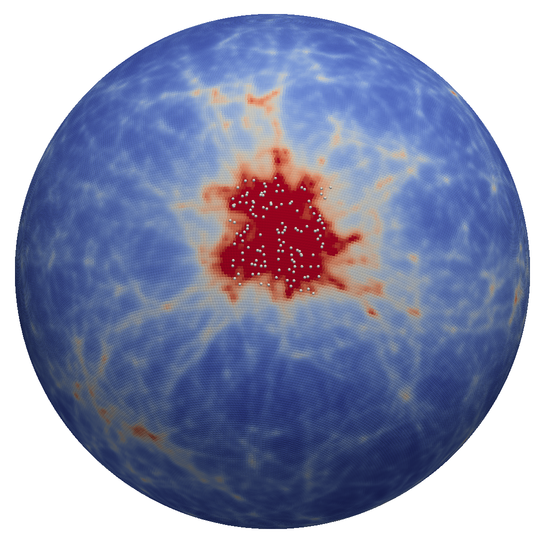
Figure 17: An illustrative example for the behaviour of the method for an extended source, 20^∘ by 20^∘. The additional 120 source neutrinos are depicted in white. The 12000 background neutrinos are not rendered. Colour indicates the $U$ values after the summation, corresponding to Figure 14.

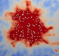
Figure 18: A zoom to the source region of Figure 17.

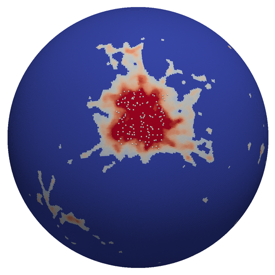
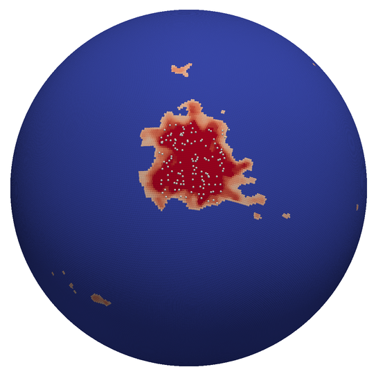
Figure 19: The results for the setup in Figure 17 after a segmentation using $\beta=0.75$ (left) and $\beta=1.11$ (right), respectively, corresponding to the $V$ values in the top panel of Figure 15.

To illustrate the behaviour of the method for a simulated extended source, the configuration shown in Figures 17 and 18 has been investigated. As shown in Figure 19, the location and size of the simulated signal are approximated reasonably well. For the result obtained with the lower $\beta$ value, however, additional filaments extend from the actual shape to regions where random accumulations of background neutrinos occurred.

The sensitivity of this method for deviations from a homogeneous spatial distribution is different compared to previously used algorithms. For instance, tests with the same simulated pseudo-experiments showed that the two-point correlation analysis [24] is more sensitive to scenarios where many faint sources with the same extension are distributed evenly throughout the sky. On the other hand, the multiscale search described here is more sensitive in scenarios that include a spatial clustering of these faint sources. It also benefits more from the presence of one or more dominant sources.

The additional information reported in [18] (pp. 95–98) verify an important aspect of the method: It only requires an increase in the number of excess events by a factor of six for an increase of the signal region from $(2\,\text{degrees})^{2}$ to $(20\,\text{degrees})^{2}$. Since a factor of ten would be expected for a constant signal-to-noise ratio, it can be concluded that the multiscale search is most sensitive to large-scale clusterings and thus has a unique sensitivity characteristic, clearly different from most other search methods.

More examples of sources, also for asymmetric shapes, and more details on the quantitative effect of neighbouring sources can be found in [18].

While the true nature of the sources of high-energy cosmic neutrinos is still unknown, this algorithm offers a high sensitivity for a wide range of possible scenarios, including ones in which many faint sources dominate the observed diffuse flux [25].

4 Results

This analysis was performed following a data blinding concept. That means that the development of all methods presented in Sections 2 and 3 and the optimisation of all cuts had been completely finished before the recorded data sample was processed. The small data sample that had been used to verify the methods was excluded from the final sample.

4.1 ANTARES

Using the methods described in Sections 2.1 and 2.2, the evaluation of the ANTARES data from 2007 to 2012 results in 13283 candidates for charged current muon neutrino events, with an expected number of background neutrinos of $13078\pm 362$ (statistical error) from interactions of cosmic rays in the atmosphere. This corresponds to a background expectation of $0.634$ neutrino candidates$/\text{degree}^{2}$. The multiscale search method described in Section 3 yields the result shown in Figure 20. Using the higher segmentation threshold $\beta=1.11$, no cluster with a significance above $0.8\sigma$ has been found. With $\beta=0.75$ a very large structure is found. After accounting for all known systematic effects, the large structure, called “the cluster” from here on, has a post-trial significance of $2.5\sigma$. The investigation of the systematic effects can be found in [18]. The size of the cluster is 13312 connected grid points, equivalent to about 3328 degree² or 8% of the sky.

The region contains about 200 events in addition to the about 2100 events expected from background. This corresponds to an excess of $0.06\pm 0.015$ neutrino candidates$/\text{degree}^{2}$. These numbers are derived assuming no subclustering within the cluster. Any subclustering (e.g. by embedded smaller clusters) would result in the same significance for a smaller average neutrino excess density. This localized event excess would not have been noticed by the two-point correlation analysis [24] nor the point source analysis and does not violate the existing bounds and observations from ANTARES and Icecube on the astrophysical diffuse flux.

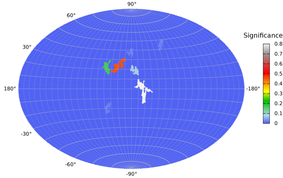
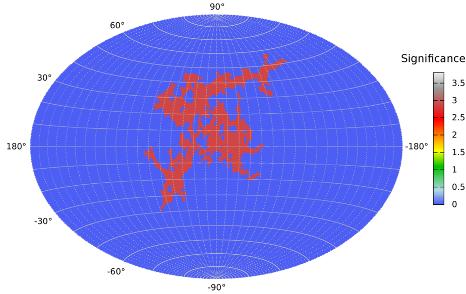
Figure 20: The result of the multiscale search for ANTARES data. The skymap is a Hammer-Aitoff projection of the resulting sphere in galactic coordinates. The colour code of the clusters indicates the post-trial significance in units of $\sigma$. Top: using $\beta=1.11$ for segmentation. Bottom: Using $\beta=0.75$.

Even if not significant on its own, this structure constitutes an interesting feature in the data which is worth further studies. It can be noted that the cluster contains the Galactic Centre, which is located in the centre of the presented skymaps in galactic coordinates. More details on the inner structure of these clusters can be seen in Figure 21, which shows the result of the summation of all scales before the segmentations. It should be noted that with the limited available statistics, random fluctuations do influence the results.

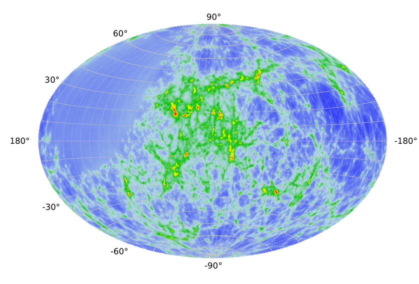
Figure 21: Top: Sum of all evaluated scales (corresponding to Figure 14, not directly to the neutrino flux) resulting from ANTARES data, in galactic coordinates and before segmentations. As only upgoing events are used in this analysis, the field of view of ANTARES does not cover the whole sky. This results in the large, homogeneously blue area in the upper left of the skymap. Bottom: For comparison, an example for a random dataset with the same colour code as the ANTARES results. The observed maximum values of $U$, see Equation 4, are similar, while the clustering of the overfluctuations is more pronounced in the recorded data.

4.2 IceCube IC40

In order to perform an independent cross check of the result obtained using ANTARES data, the publicly available IC40 dataset [26] published by the IceCube Collaboration has also been analysed. This analysis searches specifically for an excess in the area of the large cluster found in ANTARES data. To achieve this, it only considers clusters found in the IC40 data that overlap with the ANTARES cluster by at least 51% of their area. The value of 51% is chosen here because this means that they are more related to the cluster from ANTARES than to other regions. On the other hand, requiring an overlap of close to 100% would exclude e.g. clusters that extend beyond the shape of the ANTARES cluster.

Since the requirement for overlap implicitly confines the size of the cluster, the clustersize in grid points, $N_{c}$, is no reasonable metric to assess the significance of a cluster in this evaluation. Therefore the metric that gave the second best results in the investigations introduced in Section 3.8 has been used. It is the mean value of the $\sqrt{N_{c}}$ grid points with the highest values within a cluster.

The result obtained by this adapted search on the IC40 dataset is shown in Figure 22. A cluster is found within the expected shape with a post-trial significance of 2.1$\sigma$. The position of the found cluster overlaps with the search template by 78% of its size.

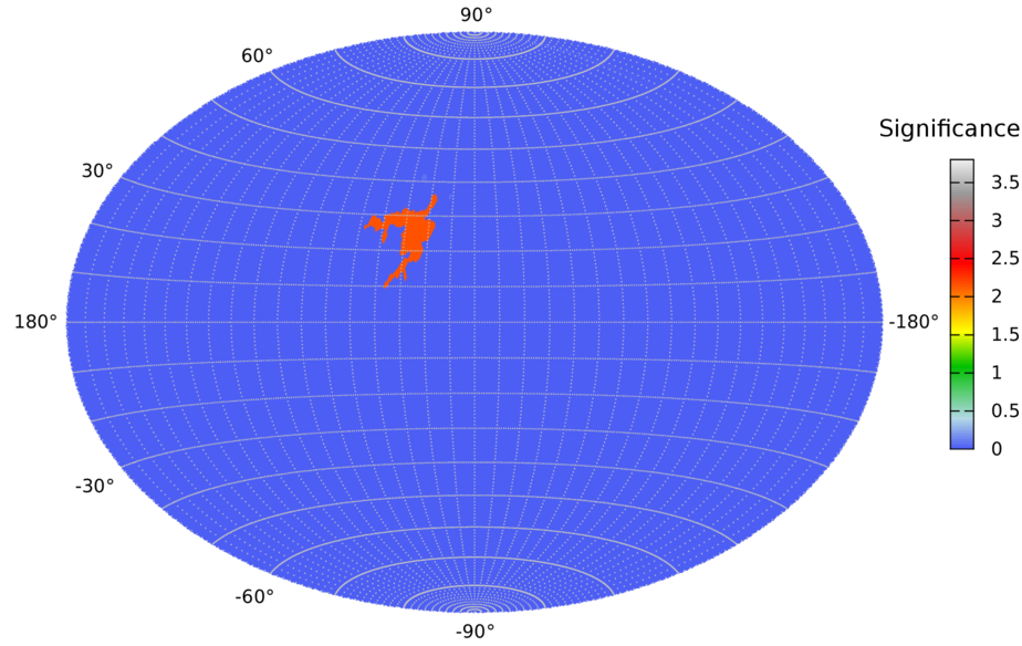
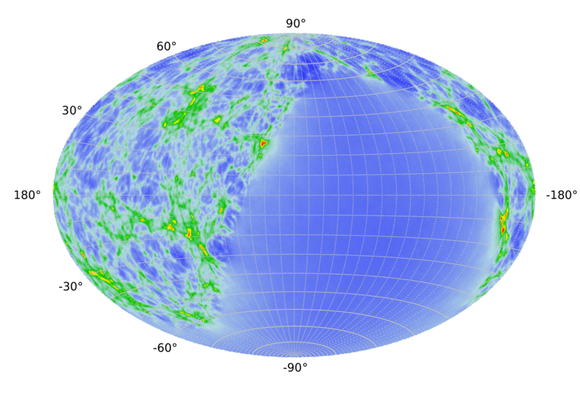
Figure 22: Top: The result on public IC40 data with segmentation using $\beta=0.75$ in galactic coordinates. Bottom: The detailed structure of $S$-values behind the result on IC40 data before the segmentation.

The observation that not all features in the skymaps in Figures 21 and 22 match exactly is to be expected, as ANTARES has its highest sensitivity at lower energies compared to IceCube. Moreover, random fluctuations of atmospheric neutrinos do influence the results.

5 Conclusions

This paper presents three original and unpublished tools that have been used for a search for cosmic neutrino sources of arbitrary location and morphology by detecting the most pronounced deviation from the background-only expectation. The study is fully data-driven, without relying on any model for neutrino emission and input derived from simulations.

The first tool (see Sect. 2.1) is a multivariate classification technique used to increasing the available statistics of ANTARES data. The second (see Sect. 2.2) enhances the directional reconstruction of charged-current muon neutrino candidates. The third tool is a model-independent multiscale method (described in Sect. 3) that represents the core of this study.

Due to the fact that the method is independent of neutrino emission models or assumptions on the topology of emission regions, this analysis is not intended to discover potential sources with the highest achievable significance, nor to analyse the properties of a candidate source region. Instead, it aims at indicating the clustering in the data least expected from the background-only hypothesis and thus to initiate more specific investigations.

Applied to ANTARES data recorded between 2007 and 2012, this analysis found a large structure with a post-trial significance of 2.5$\sigma$. This result is consistent with a random fluctuation of the background of atmospheric neutrinos. Using this method to analyse public data from IceCube resulted in an excess located within the overlap between the cluster from the ANTARES data and the field of view of IceCube. This observation has a significance of 2.1$\sigma$.

Even though a general, model-independent analysis cannot be as sensitive as a dedicated search due to the high trial factors, this method provides a good way to become aware of the most prominent and even unforeseen structures in data and can be regarded as a trigger for more specific investigations. Despite the high trial-factor, it can outperform standard point-source and two-point correlation analyses in a scenario of unknown extended structures.

References

- [1] M. G. Aartsen et al. First observation of PeV-energy neutrinos with IceCube. Phys. Rev. Lett., 111:021103, 2013.
- [2] M. G. Aartsen et al. Evidence for High-Energy Extraterrestrial Neutrinos at the IceCube Detector. Science, 342:1242856, 2013.
- [3] M. G. Aartsen et al. Atmospheric and astrophysical neutrinos above 1 TeV interacting in IceCube. Phys. Rev., D91(2):022001, 2015.
- [4] M. G. Aartsen et al. A combined maximum-likelihood analysis of the high-energy astrophysical neutrino flux measured with IceCube. Astrophys. J., 809(1):98, 2015.
- [5] M. G. Aartsen et al. Observation and characterization of a cosmic muon neutrino flux from the Northern Hemisphere using six years of IceCube data. Astrophys. J., 833(1):3, 2016.
- [6] M. G. Aartsen et al. Observation of High-Energy Astrophysical Neutrinos in Three Years of IceCube Data. Phys. Rev. Lett., 113:101101, 2014.
- [7] Andrii Neronov and Dmitry V. Semikoz. Evidence the Galactic contribution to the IceCube astrophysical neutrino flux. Astropart. Phys., 75:60–63, 2016.
- [8] A. Neronov and D. V. Semikoz. Galactic and extragalactic contributions to the astrophysical muon neutrino signal. Phys. Rev. D, 93:123002, 2016.
- [9] S. Adrián-Martínez et al. Searches for Point-like and extended neutrino sources close to the Galactic Centre using the ANTARES neutrino Telescope. Astrophys. J., 786:L5, 2014.
- [10] M. G. Aartsen et al. All-sky search for time-integrated neutrino emission from astrophysical sources with 7 years of IceCube data. Astrophys. J., 835(2):151, 2017.
- [11] S. Adrián-Martínez et al. First combined search for neutrino point-sources in the Southern Hemisphere with the ANTARES and IceCube neutrino telescopes. Astrophys. J., 823:65, 2016.
- [12] S. Adrián-Martínez et al. Searches for clustering in the time integrated skymap of the ANTARES neutrino telescope. JCAP, 1405:001, 2014.
- [13] M. G. Aartsen et al. Searches for small-scale anisotropies from neutrino point sources with three years of IceCube data. Astropart. Phys., 66:39–52, 2015.
- [14] M. Ageron et al. ANTARES: The first undersea neutrino telescope. Nucl. Inst. and Meth. A, 656(1):11–38, 2011.
- [15] S. Adrián-Martínez et al. ANTARES Constrains a Blazar Origin of Two IceCube PeV Neutrino Events. A&A, 576:L8, 2015.
- [16] Bystritsky, V. and Bochkanov, S. (The ALGLIB Project). ALGLIB. http://www.alglib.net, 2011. 2011-11.
- [17] Tin Kam Ho. The Random Subspace Method for Constructing Decision Forests. IEEE Transactions on Pattern Analysis and Machine Intelligence, 20:832–844, 1998.
- [18] Stefan Geißelsöder. Model-independent search for neutrino sources with the ANTARES neutrino telescope. Ph.D. thesis, Friedrich-Alexander-Universität Erlangen-Nürnberg, 2016. https://opus4.kobv.de/opus4-fau/files/6997/dissertation_geisselsoeder.pdf (in English, preface in German).
- [19] L.A. Fusco et al. The Run-by-Run Monte Carlo simulation for the ANTARES experiment. EPJ Web of Conf., 116:02002, 2016.
- [20] S. Adrián-Martínez et al. First Search for Point Sources of High Energy Cosmic Neutrinos with the ANTARES Neutrino Telescope. Astrophys. J. Lett., L14:743, 2011.
- [21] J.A. Aguilar et al. A fast algorithm for muon track reconstruction and its application to the ANTARES neutrino Telescope. Astropart. Phys., 34:652–662, 2011.
- [22] Erwin Lourens Visser. Neutrinos from the Milky Way. Ph.D. thesis, Universiteit Leiden, 2015. http://www.nikhef.nl/pub/services/biblio/theses_pdf/thesis_EL_Visser.pdf.
- [23] S. Adrián-Martínez et al. Search for Cosmic Neutrino Point Sources with Four Year Data of the ANTARES Telescope. Astrophys. J., 760:53, 2012.
- [24] S. Adrián-Martínez et al. Searches for clustering in the time integrated skymap of the ANTARES neutrino telescope. JCAP, 05:001, 2014.
- [25] M. G. Aartsen et al. Astrophysical neutrinos and cosmic rays observed by IceCube. Adv. Space Res., 62:2902, 2018.
- [26] R. Abbasi et al. A Search for a Diffuse Flux of Astrophysical Muon Neutrinos with the IceCube 40-String Detector. Phys. Rev. D, 84:082001, 2011. http://icecube.wisc.edu/science/data/ic40.