Quantum kinetic equations for the ultrafast spin dynamics of excitons in diluted magnetic semiconductor quantum wells after optical excitation

Abstract

Quantum kinetic equations of motion for the description of the exciton spin dynamics in II-VI diluted magnetic semiconductor quantum wells with laser driving are derived. The model includes the magnetic as well as the nonmagnetic carrier-impurity interaction, the Coulomb interaction, Zeeman terms, and the light-matter coupling, allowing for an explicit treatment of arbitrary excitation pulses. Based on a dynamics-controlled truncation scheme, contributions to the equations of motion up to second order in the generating laser field are taken into account. The correlations between the carrier and the impurity subsystems are treated within the framework of a correlation expansion. For vanishing magnetic field, the Markov limit of the quantum kinetic equations formulated in the exciton basis agrees with existing theories based on Fermi’s golden rule. For narrow quantum wells excited at the $1s$ exciton resonance, numerical quantum kinetic simulations reveal pronounced deviations from the Markovian behavior. In particular, the spin decays initially with approximately half the Markovian rate and a non-monotonic decay in the form of an overshoot of up to $10\,\%$ of the initial spin polarization is predicted.

I Introdction

The idea behind the spintronics paradigmDietl (2010); Ohno (2010); Žutić et al. (2004); Awschalom and Flatté (2007) is to combine state-of-the-art electronics based on carrier charge with the manipulation and control of the spin degree of freedomAwschalom et al. (2013); Wunderlich et al. (2010); Chappert et al. (2007). Diluted magnetic semiconductors (DMS)Dietl and Ohno (2014); Kossut and Gaj (2010); Furdyna (1988) present an interesting subclass of semiconductors in this context because they can be easily combined with current semiconductor technology while at the same time providing a wide range of spin and magnetization-related effects and applications Kossut (1975); Bastard and Ferreira (1992); Cywiński and Sham (2007); Nawrocki et al. (1981); Kapetanakis et al. (2012); Das Sarma et al. (2003); Camilleri et al. (2001); Krenn et al. (1989); Debus et al. (2016); Awschalom and Samarth (1999); Crooker et al. (1997); Baumberg et al. (1994). In DMS, a small fraction of magnetic ions, usually ManganeseFurdyna and Kossut (1988), is introduced into a semiconductor. While III-V compounds such as Ga_1-xMn_xAs are typically p-dopedDietl and Ohno (2014) and can thus exhibit carrier-mediated ferromagnetismOhno et al. (1996), II-VI materials such as Cd_1-xMn_xTe are found to be intrinsic and paramagnetic due to the isoelectrical incorporation of the Mn impurities.

A lot of theoretical works on DMS has been devoted to the understanding of structural propertiesJungwirth et al. (2006a, 2002, 2005, b, 2010); Bouzerar and Bouzerar (2010). But in many experiments, also the spin dynamics studied via optical pump-probe experiments is of interestBen Cheikh et al. (2013); Camilleri et al. (2001); Krenn et al. (1989). Theoretical descriptions of such experiments are less developed in the literature and are typically based on rate-equation modelsBastard and Ferreira (1992); Cywiński and Sham (2007); Nawrocki et al. (1981); Camilleri et al. (2001); Ben Cheikh et al. (2013); Semenov and Kirichenko (1996); Semenov (2003); Jiang et al. (2009); Vladimirova et al. (2008), coinciding with Fermi’s golden rule for vanishing magnetic field. However, a number of experiments have provided strong evidence that these models fail to reproduce some of the pertinent characteristics of the spin dynamics in DMS. Most notably, experimentally observed spin-decay rates are found to be a factor of $5$ larger than the Fermi’s golden rule result for spin-flip scattering of conduction band electrons at magnetic impuritiesBen Cheikh et al. (2013). Camilleri et al.Camilleri et al. (2001) have argued that their optical experiments probe excitons rather than separate electrons and holes. In this case, the effective mass entering the spin-flip rate has to be replaced by the exciton massBastard and Ferreira (1992), offering a potential explanation for the discrepancy noted in Ref. Ben Cheikh et al., 2013.

On the rate-equation level, some groups have already investigated the exciton spin dynamics in DMS theoreticallyTsitsishvili and Kalt (2006); Maialle et al. (1993); Maialle and Sham (1994); Selbmann et al. (1996); Tang et al. (2015); Adachi et al. (1997). However, recent studies using a quantum kinetic theory for the spin relaxation of conduction band electrons in DMS revealed that correlations between the carrier and impurity subsystems can induce a finite memoryThurn and Axt (2012); Cygorek et al. (2016a, 2017, b) which is not captured by rate equations. The resulting non-Markovian effects were found to be particularly pronounced for excitations close to the band edge ($\mathbf{k}\approx\mathbf{0}$)Cygorek and Axt (2015) and become more significant with increasing effective massThurn et al. (2013). These tendencies suggest that non-Markovian features are particularly relevant for excitons since, first of all, the conservation of momentum implies a vanishing center of mass momentum ($\mathbf{K}\approx\mathbf{0}$) of optically generated excitons, and second, the exciton mass is much larger than the effective mass of conduction band electrons.

In this article, we develop a microscopic quantum kinetic theory for the exciton spin dynamics in DMS that is also capable of describing non-Markovian effects by explicitly accounting for carrier-impurity correlations. In contrast to previous worksThurn and Axt (2012) where independent electrons and holes were considered and where higher-order correlations were treated within a variant of Kubo’s cumulant expansionKubo (1962), here a dynamics-controlled truncation (DCT)Axt and Stahl (1994); Axt and Mukamel (1998) is employed for the treatment of Coulomb correlations. This approach is especially advantageous for the description of optically-driven systems since it ensures a correct description of the dynamics up to a given order in the generating field. The theory derived in this paper is applicable in a wide range of different scenarios as a number of interactions are accounted for, such as the magnetic and nonmagnetic interactions between impurities and electrons as well as holes, the Coulomb interaction responsible for the formation of excitons, Zeeman terms for electrons, holes, and impurities, as well as the light-matter coupling.

Moreover, we show that, in the Markov limit and for vanishing magnetic field, the quantum kinetic description coincides with the Fermi’s golden rule result of Ref. Bastard and Ferreira, 1992. Comparing numerical simulations using the quantum kinetic theory and Markovian rate equations reveals strong non-Markovian effects in the exciton spin dynamics. In particular, the quantum kinetic calculations predict that the exciton spin initially decays with approximately half the rate obtained from Fermi’s golden rule and exhibits a nonmonotonic behavior with an overshoot of up to $10\,\%$ of the initial spin polarization. In contrast to the situation for conduction band electrons, where nonmagnetic impurity scattering typically strongly suppresses non-Markovian featuresCygorek et al. (2017), here we find that, for excitons, the presence of nonmagnetic impurity scattering enhances the characteristics of non-Markovian behavior.

The article is structured as follows: First, we discuss the individual contributions to the Hamiltonian that determines the spin dynamics of optically generated excitons in DMS quantum wells. Next, quantum kinetic equations based on a DCT scheme are derived for reduced exciton and impurity density matrices as well as carrier-impurity correlations. We then derive the Markov limit of the quantum kinetic equations of motion. Finally, we present numerical calculations and discuss the results.

II Theory

In this section, we present the Hamiltonian that models the optical excitation and the subsequent spin evolution of excitons in II-VI DMS. We explain the derivation of the quantum kinetic equations and, for comparison, also give the Markov limit of the equations.

II.1 Hamiltonian

We consider an intrinsic II-VI DMS quantum well where initially no electrons are in the conduction band. The time evolution of the system can then be described by the Hamiltonian

$$H =H_{0}^{\textrm{e}}+H_{0}^{\textrm{h}}+H_{\textrm{conf}}+H_{\textrm{C}}+H_{\textrm{Z}}^{\textrm{e}}+H_{\textrm{Z}}^{\textrm{h}}+H_{\textrm{Z}}^{\textrm{Mn}}+H_{\textrm{lm}}$$

$$\phantom{=\;}+H_{sd}+H_{pd}+H_{\textrm{nm}}^{\textrm{e}}+H_{\textrm{nm}}^{\textrm{h}},$$ (1)

where

$$H_{0}^{\textrm{e}}+H_{0}^{\textrm{h}} =\sum_{l\mathbf{k}}E^{l}_{\mathbf{k}}c^{\dagger}_{l\mathbf{k}}c_{l\mathbf{k}}+\sum_{v\mathbf{k}}E^{v}_{\mathbf{k}}d^{\dagger}_{v\mathbf{k}}d_{v\mathbf{k}}$$ (2)

is the crystal Hamiltonian for electrons and holes, respectively. Here, $c^{\dagger}_{l\mathbf{k}}$ ($c_{l\mathbf{k}}$) denotes the creation (annihilation) operator of an electron in the conduction band $l$ with wave vector $\mathbf{k}$. Similarly, $d^{\dagger}_{v\mathbf{k}}$ ($d_{v\mathbf{k}}$) creates (annihilates) a hole in the valence band $v$. The confinement potentials for electrons and holes responsible for the formation of a quantum well is denoted by $H_{\textrm{conf}}$.

As usual for the description of near band-edge excitations of semiconductors we consider the part of the Coulomb interaction conserving the number of electrons and holes, which corresponds to the typically dominant monopole-monopole part in a multipolar expansionHaken (1976); Axt and Mukamel (1998); Stahl (1988); Huhn and Stahl (1984). The Coulomb interaction then reads

$$H_{\textrm{C}}=\frac{1}{2}\sum_{\mathbf{k}\mathbf{k}^{\prime}\mathbf{q}}\Big{(} V_{\mathbf{q}}\sum_{ll^{\prime}}c^{\dagger}_{l^{\prime}\mathbf{k}^{\prime}+\mathbf{q}}c^{\dagger}_{l\mathbf{k}-\mathbf{q}}c_{l\mathbf{k}}c_{l^{\prime}\mathbf{k}^{\prime}}$$

$$+V_{\mathbf{q}}\sum_{vv^{\prime}}d^{\dagger}_{v^{\prime}\mathbf{k}^{\prime}+\mathbf{q}}d^{\dagger}_{v\mathbf{k}-\mathbf{q}}d_{v\mathbf{k}}d_{v^{\prime}\mathbf{k}^{\prime}}$$

$$-2V_{\mathbf{q}}\sum_{lv}c^{\dagger}_{l\mathbf{k}^{\prime}+\mathbf{q}}d^{\dagger}_{v\mathbf{k}-\mathbf{q}}d_{v\mathbf{k}}c_{l\mathbf{k}^{\prime}}\Big{)}$$ (3)

with the Fourier transform of the Coulomb potential given by $V_{\mathbf{q}}=\frac{e^{2}}{\epsilon\epsilon_{0}}\frac{1}{q^{2}}$, where $e$ is the elementary charge and $\epsilon_{0}$ is the vacuum permittivity. The dielectric constant $\epsilon\approx 10$ includes the contribution of the crystal latticeRashba and Sturge (1982); Strzalkowski et al. (1976). Thus, $H_{\textrm{C}}$ comprises all direct electron-electron, hole-hole, and electron-hole Coulomb interactions.

We account for the effects of a homogeneous external magnetic field $\mathbf{B}$ on the electrons, holes, and magnetic impurity atoms, respectively, via the Zeeman terms

$$H_{\textrm{Z}}^{\textrm{e}} =g_{\textrm{e}}\mu_{B}\sum_{ll^{\prime}\mathbf{k}}\mathbf{B}\cdot\mathbf{s}^{\textrm{e}}_{ll^{\prime}}c^{\dagger}_{l\mathbf{k}}c_{l^{\prime}\mathbf{k}},\allowdisplaybreaks$$ (4a)

$$H_{\textrm{Z}}^{\textrm{h}} =-2\kappa\mu_{B}\sum_{vv^{\prime}\mathbf{k}}\mathbf{B}\cdot\mathbf{J}_{vv^{\prime}}d^{\dagger}_{v\mathbf{k}}d_{v^{\prime}\mathbf{k}},\allowdisplaybreaks$$ (4b)

$$H_{\textrm{Z}}^{\textrm{Mn}} =g_{\textrm{Mn}}\mu_{B}\sum_{Inn^{\prime}}\mathbf{B}\cdot\mathbf{S}_{nn^{\prime}}\hat{P}^{I}_{nn^{\prime}}.$$ (4c)

In the above formulas, $g_{\textrm{e}}$ is the $g$ factor of the electrons, $\kappa$ is the isotropic valence-band $g$ factorWinkler (2003), $g_{\textrm{Mn}}$ denotes the impurity $g$ factor, and $\mu_{B}$ is the Bohr magneton. The vector of electron-spin matrices is given by $\mathbf{s}^{\textrm{e}}_{ll^{\prime}}$, $\mathbf{J}_{vv^{\prime}}$ is the vector of $4\times 4$ angular momentum matrices when accounting for heavy hole (hh) and light hole (lh) bands with angular momentum $v,v^{\prime}\in\{-\frac{3}{2},-\frac{1}{2},\frac{1}{2},\frac{3}{2}\}$ and $\mathbf{S}_{nn^{\prime}}$ denotes the vector of impurity spin matrices. In the case of manganese considered here, we have $n,n^{\prime}\in\{-\frac{5}{2},-\frac{3}{2},...,\frac{5}{2}\}$. The impurity spin itself is described by the operator $\hat{P}^{I}_{nn^{\prime}}=|I,n\rangle\langle I,n^{\prime}|$ where the ket $|I,n\rangle$ denotes the spin state $n$ of an impurity atom $I$.

Rather than assuming some initial carrier distribution, we explicitly account for the optical excitation and thus the light-matter coupling via the Hamiltonian

$$H_{\textrm{lm}}=-\sum_{lv\mathbf{k}}\left(\mathbf{E}\cdot\mathbf{M}_{lv}c^{\dagger}_{l\mathbf{k}}d^{\dagger}_{v-\mathbf{k}}+\mathbf{E}\cdot\mathbf{M}_{vl}d_{v-\mathbf{k}}c_{l\mathbf{k}}\right)$$ (5)

with an electric field $\mathbf{E}$ and the dipole moment $\mathbf{M}_{lv}$ for a transition from a state in the valence subband $v$ to the conduction subband $l$. Here, the well-known dipole approximationRossi and Kuhn (2002) is used to consider only interband transitions with vanishing center of mass momentum.

The dominant spin depolarization mechanism in DMS is given by the $sp$-$d$ exchange interaction which models the scattering of $s$-like conduction-band electrons and $p$-like valence-band holes, respectively, at the localized $d$-shell electrons of the Mn impurities. These interactions can be written asDietl and Ohno (2014); Kossut and Gaj (2010); Cygorek et al. (2016a)

$$H_{sd} =\frac{J_{sd}}{V}\sum_{\begin{subarray}{c}Inn^{\prime}\\ ll^{\prime}\mathbf{k}\mathbf{k}^{\prime}\end{subarray}}\mathbf{S}_{nn^{\prime}}\cdot\mathbf{s}^{\textrm{e}}_{ll^{\prime}}c^{\dagger}_{l\mathbf{k}}c_{l^{\prime}\mathbf{k}^{\prime}}e^{i(\mathbf{k}^{\prime}-\mathbf{k})\cdot\mathbf{R}_{I}}\!\hat{P}^{I}_{nn^{\prime}},\allowdisplaybreaks$$ (6a)

$$H_{pd} =\frac{J_{pd}}{V}\sum_{\begin{subarray}{c}Inn^{\prime}\\ vv^{\prime}\mathbf{k}\mathbf{k}^{\prime}\end{subarray}}\mathbf{S}_{nn^{\prime}}\cdot\mathbf{s}^{\textrm{h}}_{vv^{\prime}}d^{\dagger}_{v\mathbf{k}}d_{v^{\prime}\mathbf{k}^{\prime}}e^{i(\mathbf{k}^{\prime}-\mathbf{k})\cdot\mathbf{R}_{I}}\!\hat{P}^{I}_{nn^{\prime}}$$ (6b)

with the hole spin matrices given by $\mathbf{s}^{\textrm{h}}_{vv^{\prime}}=\frac{1}{3}\mathbf{J}_{vv^{\prime}}$. Note that we employ the convention that the factor $\hbar$ which typically enters in the definition of the spin matrices is instead absorbed in the coupling constants $J_{sd}$ and $J_{pd}$ as well as $\mu_{B}$ in case of the Zeeman terms.

In a recently published paper it was shown that the combined action of nonmagnetic impurity scattering and magnetic exchange interaction may have a significant impact on the spin dynamics of conduction band electronsCygorek et al. (2017). Therefore, we also include the nonmagnetic impurity scattering in the form

$$H_{\textrm{nm}}^{\textrm{e}} =\frac{J_{0}^{\textrm{e}}}{V}\sum_{\begin{subarray}{c}Il\\ \mathbf{k}\mathbf{k}^{\prime}\end{subarray}}c^{\dagger}_{l\mathbf{k}}c_{l\mathbf{k}^{\prime}}e^{i(\mathbf{k}^{\prime}-\mathbf{k})\cdot\mathbf{R}_{I}},\allowdisplaybreaks$$ (7a)

$$H_{\textrm{nm}}^{\textrm{h}} =\frac{J_{0}^{\textrm{h}}}{V}\sum_{\begin{subarray}{c}Iv\\ \mathbf{k}\mathbf{k}^{\prime}\end{subarray}}d^{\dagger}_{v\mathbf{k}}d_{v\mathbf{k}^{\prime}}e^{i(\mathbf{k}^{\prime}-\mathbf{k})\cdot\mathbf{R}_{I}}$$ (7b)

with scattering constants $J_{0}^{\textrm{e}}$ and $J_{0}^{\textrm{h}}$ for electrons and holes, respectively. Considering a DMS of the general form A_1-xMn_xB, these can be determined under the assumption that unit cells containing doping ions experience an energetic penalty due to being forced into the same structure as the surrounding semiconductor lattice AB. This allows for an estimation of the nonmagnetic coupling strength based on the change of the band gap of the pure AB material compared to the pure MnB material. Note that we only take into account the short-range part of the carrier-impurity interaction even though it stems largely from the Coulomb interaction between the impurity atoms and the quasi-free carriersCygorek et al. (2017).

We do not include the influence of phonons on the carrier spin dynamics in our model since typical experimentsBen Cheikh et al. (2013); Camilleri et al. (2001); Vladimirova et al. (2008) are performed at low temperatures of about $2\,$K where only phonon emission is relevant because there are no phonons available for absorption. But since we consider only direct laser-driven excitation of excitons with vanishing center of mass momenta, phonon emission processes are also strongly suppressed as there are no final exciton states lower in energy to scatter to. Additionally, phonons do not couple directly to the spin and thus represent a secondary relaxation process which only becomes relevant in combination with other effects, such as spin-orbit coupling. Theoretical rate-equation models that include the scattering due to phonons also support that the $s$-$d$ exchange interaction is the most important scattering mechanism at low temperaturesJiang et al. (2009). Given that the recently reportedDebus et al. (2016) spin-lattice relaxation time of Mn²⁺ ions in typical DMS quantum wells is on the order of $\mu$s, the coupling of phonons to the Mn system can also be disregarded on the typical ps time scale of the carrier spin relaxationCygorek et al. (2017); Ungar et al. (2015); Ben Cheikh et al. (2013). Furthermore, spin-orbit effectsUngar et al. (2015) as well as the hyperfine interactionWu et al. (2010) due to nuclear spins typically also only become relevant at much longer time scales.

In a quantum well, it is convenient to switch from a three-dimensional basis set to a description where only the in-plane part consists of plane waves and the $z$ dependence is treated separately. One can then expand the single-particle basis functions $\Xi$ in terms of a complete set of envelope functions, which yields

$$\Xi(\mathbf{r},z)=\frac{1}{\sqrt{A}}\sum_{n\mathbf{k}}a_{n\mathbf{k}}e^{i\mathbf{k}\cdot\mathbf{r}}\,u_{n}^{\textrm{e/h}}(z)$$ (8)

with envelope functions $u_{n}^{\textrm{e/h}}(z)$ of electrons and holes, respectively, and expansion coefficients $a_{n\mathbf{k}}$. Here and throughout the remainder of this article, the appearing wave vectors $\mathbf{k}$ as well as the in-plane position $\mathbf{r}$ are two-dimensional quantities.

For narrow quantum wells, where the energetic separation between the individual confinement states is large, it is a good approximation to only consider the lowest confinement stateAstakhov et al. (2002) $u_{0}^{\textrm{e/h}}(z)$, which corresponds to setting $a_{n\mathbf{k}}=0$ for all $n\neq 0$. Thus, we project the Hamiltonian given by Eq. (II.1) onto the corresponding subspace. For the carrier-impurity interactions in Eqs. (6) and (7), this amounts to substituting $\sum_{k_{z}k_{z}^{\prime}}\to d|u_{0}^{\textrm{e/h}}(Z_{I})|^{2}$. In numerical calculations, we assume infinitely high potential barriers at $z=\pm\frac{d}{2}$, so that the envelope functions for electrons and holes become

$$u_{0}^{\textrm{e/h}}(z)=\sqrt{\frac{2}{d}}\cos\Big{(}\frac{\pi}{d}z\Big{)}.$$ (9)

II.2 Dynamical variables and truncation scheme

Our main target is the modeling of the electron or hole spin dynamics in a system where all particles are excited optically as electron-hole pairs. Within the DCT scheme this is most conveniently achieved by deriving quantum kinetic equations of motion for the four-point density matrices $\langle c^{\dagger}_{l_{1}\mathbf{k}_{1}}d^{\dagger}_{v_{1}\mathbf{k}_{2}}d_{v_{2}\mathbf{k}_{3}}c_{l_{2}\mathbf{k}_{4}}\rangle$ from which all relevant information can be deducedAxt and Mukamel (1998). To provide an example, the electron density matrix is given by

$$\langle c^{\dagger}_{l_{1}\mathbf{k}_{1}}c_{l_{2}\mathbf{k}_{2}}\rangle =\sum_{v\mathbf{k}}\langle c^{\dagger}_{l_{1}\mathbf{k}_{1}}d^{\dagger}_{v\mathbf{k}}d_{v\mathbf{k}}c_{l_{2}\mathbf{k}_{2}}\rangle+\mathcal{O}(\mathbf{E}^{4}).$$ (10)

Starting from the Hamiltonian given by Eq. (II.1) and using the Heisenberg equation of motion, one ends up with an infinite hierarchy of equations that needs to be truncated in order to be solvable. In this article, we employ a dynamics-controlled truncationAxt and Stahl (1994) which classifies all appearing expectation values in terms of their order in the generating optical field. Using this procedure, we keep all contributions up to the order $\mathcal{O}(\mathbf{E}^{2})$, which is sufficient in the low-density regimeSiantidis et al. (2001).

However, since we are dealing with a DMS, we also have to treat correlations between carriers and Mn atoms. This is done using a correlation expansion similarly to Ref. Thurn and Axt, 2012 where, due to the Mn atoms being far apart in a DMS, correlations that involve magnetic dopants at different sites are disregarded. Applications of correlation expansions in condensed matter physics are manifold and can be found explained numerous times in the literatureZimmermann and Wauer (1994); Rossi and Kuhn (2002); Thurn and Axt (2012); Kira and Koch (2008, 2006); Kuhn (1998).

Setting up the equations of motion for an on-average spatially homogeneous system, a closed set of equations of motion can be formulated for the following dynamical variables:

$$M_{n_{1}}^{n_{2}}(z) =\frac{d}{N_{\textrm{Mn}}}\sum_{I}\delta(z-Z_{I})\big{\langle}\hat{P}_{n_{1}n_{2}}^{I}\big{\rangle},\allowdisplaybreaks$$ (11a)

$$Y_{\mathbf{k}_{1}}^{v_{1}l_{1}} =\big{\langle}d_{v_{1}-\mathbf{k}_{1}}c_{l_{1}\mathbf{k}_{1}}\big{\rangle},\allowdisplaybreaks$$ (11b)

$$N_{\mathbf{k}_{1}\mathbf{k}_{2}\mathbf{k}_{3}\mathbf{k}_{4}}^{l_{1}v_{1}v_{2}l_{2}} =\big{\langle}c^{\dagger}_{l_{1}\mathbf{k}_{1}}d^{\dagger}_{v_{1}-\mathbf{k}_{2}}d_{v_{2}-\mathbf{k}_{3}}c_{l_{2}\mathbf{k}_{4}}\big{\rangle}\delta_{\mathbf{k}_{1}-\mathbf{k}_{2},\mathbf{k}_{4}-\mathbf{k}_{3}},\allowdisplaybreaks$$ (11c)

$${Q_{Y}}_{n_{1}\mathbf{k}_{1}\mathbf{k}_{2}}^{n_{2}v_{1}l_{1}}(z) =V\frac{d}{N_{\textrm{Mn}}}\sum_{I}\delta(z-Z_{I})\big{\langle}d_{v_{1}-\mathbf{k}_{1}}c_{l_{1}\mathbf{k}_{2}}e^{i(\mathbf{k}_{2}-\mathbf{k}_{1})\cdot\mathbf{R}_{I}}\hat{P}_{n_{1}n_{2}}^{I}\big{\rangle}\textrm{, for }\mathbf{k}_{1}\neq\mathbf{k}_{2},\allowdisplaybreaks$$ (11d)

$$\bar{Y}_{\mathbf{k}_{1}\mathbf{k}_{2}}^{v_{1}l_{1}}(z) =V\frac{d}{N_{\textrm{Mn}}}\sum_{I}\delta(z-Z_{I})\big{\langle}d_{v_{1}-\mathbf{k}_{1}}c_{l_{1}\mathbf{k}_{2}}e^{i(\mathbf{k}_{2}-\mathbf{k}_{1})\cdot\mathbf{R}_{I}}\big{\rangle}\textrm{, for }\mathbf{k}_{1}\neq\mathbf{k}_{2},\allowdisplaybreaks$$ (11e)

$${Q_{N}}_{n_{1}\mathbf{k}_{1}\mathbf{k}_{2}\mathbf{k}_{3}\mathbf{k}_{4}}^{n_{2}l_{1}v_{1}v_{2}l_{2}}(z) =V\frac{d}{N_{\textrm{Mn}}}\sum_{I}\delta(z-Z_{I})\big{\langle}c^{\dagger}_{l_{1}\mathbf{k}_{1}}d^{\dagger}_{v_{1}-\mathbf{k}_{2}}d_{v_{2}-\mathbf{k}_{3}}c_{l_{2}\mathbf{k}_{4}}e^{i(\mathbf{k}_{2}-\mathbf{k}_{1}+\mathbf{k}_{4}-\mathbf{k}_{3})\cdot\mathbf{R}_{I}}\hat{P}_{n_{1}n_{2}}^{I}\big{\rangle}\textrm{, for }\mathbf{k}_{1}-\mathbf{k}_{2}\neq\mathbf{k}_{4}-\mathbf{k}_{3},\allowdisplaybreaks$$ (11f)

$$\bar{N}_{\mathbf{k}_{1}\mathbf{k}_{2}\mathbf{k}_{3}\mathbf{k}_{4}}^{l_{1}v_{1}v_{2}l_{2}} =V\frac{d}{N_{\textrm{Mn}}}\sum_{I}\delta(z-Z_{I})\big{\langle}c^{\dagger}_{l_{1}\mathbf{k}_{1}}d^{\dagger}_{v_{1}-\mathbf{k}_{2}}d_{v_{2}-\mathbf{k}_{3}}c_{l_{2}\mathbf{k}_{4}}e^{i(\mathbf{k}_{2}-\mathbf{k}_{1}+\mathbf{k}_{4}-\mathbf{k}_{3})\cdot\mathbf{R}_{I}}\big{\rangle}\textrm{, for }\mathbf{k}_{1}-\mathbf{k}_{2}\neq\mathbf{k}_{4}-\mathbf{k}_{3}.$$ (11g)

In the above equations, $M_{n_{1}}^{n_{2}}(z)$, $Y_{\mathbf{k}_{1}}^{v_{1}l_{1}}$, and $N_{\mathbf{k}_{1}\mathbf{k}_{2}\mathbf{k}_{3}\mathbf{k}_{4}}^{l_{1}v_{1}v_{2}l_{2}}$ represent the Mn density matrices, the electron-hole coherences, and the exciton density matrices, respectively. The magnetic and nonmagnetic correlations between coherences and impurity atoms are given by ${Q_{Y}}_{n_{1}\mathbf{k}_{1}\mathbf{k}_{2}}^{n_{2}v_{1}l_{1}}(z)$ and $\bar{Y}_{\mathbf{k}_{1}\mathbf{k}_{2}}^{v_{1}l_{1}}(z)$, respectively, and in turn by ${Q_{N}}_{n_{1}\mathbf{k}_{1}\mathbf{k}_{2}\mathbf{k}_{3}\mathbf{k}_{4}}^{n_{2}l_{1}v_{1}v_{2}l_{2}}(z)$ and $\bar{N}_{\mathbf{k}_{1}\mathbf{k}_{2}\mathbf{k}_{3}\mathbf{k}_{4}}^{l_{1}v_{1}v_{2}l_{2}}$ between excitons and impurities. In addition to the usual quantum mechanical average of the operators, the brackets $\langle.\rangle$ in Eqs. (11) as well as throughout the rest of this paper also contain an average over the distribution of Mn positions in the sample. This distribution is assumed to be random but homogeneous on average, so that $\langle e^{i(\mathbf{k}_{2}-\mathbf{k}_{1})\cdot\mathbf{R}_{I}}\rangle=\delta_{\mathbf{k}_{1},\mathbf{k}_{2}}$. The delta distribution in Eq. (11c) is a consequence of the spatial homogeneity of the system.

Using these variables, it is straightforward but lengthy to set up a hierarchy of equations of motion whilst retaining only terms up to $\mathcal{O}(\mathbf{E}^{2})$ according to the DCT scheme. However, it turns out that the magnetic interactions $H_{sd}$ and $H_{pd}$ introduce additional source terms in the equations for the correlations that are not expressible using the variables from Eqs. (11) because they contain products of Mn operators as well as exponential functions containing the randomly distributed Mn positions $\mathbf{R}_{I}$ in the exponent. Following along the lines of Ref. Thurn and Axt, 2012, where a correlation expansion has been successfully employed to treat these terms, we sketch the general method of such an expansion when applied to the expressions derived in this paper. Our approach for dealing with random impurity positions can also be related to the treatment of interface roughness via random potentials as well as the influence of disorder in semiconductorsZimmermann and Runge (1994); Zimmermann (1992, 1995).

Consider a general expectation value of the form

$$S_{Q} =\langle Xe^{i\Delta\mathbf{k}\cdot\mathbf{R}_{I}}e^{i\Delta\mathbf{k}^{\prime}\cdot\mathbf{R}_{I^{\prime}}}\hat{P}_{n_{1}n_{2}}^{I}\hat{P}_{n_{1}^{\prime}n_{2}^{\prime}}^{I^{\prime}}\rangle,$$ (12)

where $X$ contains up to four Fermi operators so that $\langle X\rangle$ is up to $\mathcal{O}(E^{2})$ and $\Delta\mathbf{k}\neq\mathbf{0}$. Using the DCT scheme, it can be easily shown that assisted expectation values such as the quantity in Eq. (12) are of the same order in the generating electric field as the corresponding bare expectation values of the Fermi operators. We then treat the expression in Eq. (12) as follows:

(i) The situation $I=I^{\prime}$ has to be considered separately since in this case we are dealing with Mn operators on the same site, so that Eq. (12) reduces to

$$S_{Q}\stackrel{{\scriptstyle I=I^{\prime}}}{{=}}\langle Xe^{i(\Delta\mathbf{k}+\Delta\mathbf{k}^{\prime})\cdot\mathbf{R}_{I}}\hat{P}_{n_{1}n_{2}^{\prime}}^{I}\rangle\delta_{n_{2},n_{1}^{\prime}}$$ (13)

in accordance with the definition of the Mn operators $\hat{P}_{nn^{\prime}}^{I}$. The remaining quantity can then be expressed in terms of the variables introduced in Eq. (11).

(ii) If $\Delta\mathbf{k}^{\prime}=\mathbf{0}$, we get

$$S_{Q}\stackrel{{\scriptstyle\Delta\mathbf{k}^{\prime}=\mathbf{0}}}{{=}}\langle Xe^{i\Delta\mathbf{k}\cdot\mathbf{R}_{I}}\hat{P}_{n_{1}n_{2}}^{I}\hat{P}_{n_{1}^{\prime}n_{2}^{\prime}}^{I^{\prime}}\rangle,$$ (14)

so that the number of operators effectively is reduced by one.

(iii) In the most general case, i.e., $I\neq I^{\prime}$ and $\Delta\mathbf{k}^{\prime}\neq 0$, we decompose Eq. (12) using a correlation expansion. This yields

$$S_{Q} =\delta\langle Xe^{i\Delta\mathbf{k}\cdot\mathbf{R}_{I}}\hat{P}_{n_{1}n_{2}}^{I}\rangle\langle e^{i\Delta\mathbf{k}^{\prime}\cdot\mathbf{R}_{I^{\prime}}}\rangle\langle\hat{P}_{n_{1}^{\prime}n_{2}^{\prime}}^{I^{\prime}}\rangle$$

$$\phantom{=\;}+\delta\langle Xe^{i\Delta\mathbf{k}\cdot\mathbf{R}_{I}}\rangle\langle\hat{P}_{n_{1}n_{2}}^{I}\rangle\langle e^{i\Delta\mathbf{k}^{\prime}\cdot\mathbf{R}_{I^{\prime}}}\rangle\langle\hat{P}_{n_{1}^{\prime}n_{2}^{\prime}}^{I^{\prime}}\rangle$$ (15)

with true correlations denoted by $\delta\langle...\rangle$. In the above equation, we have only written down the non-vanishing terms of the expansion by neglecting correlations evaluated either at different Mn sites or involving two or more impurity operators. Furthermore, it can be shown that correlations of the form $\delta\langle e^{i\Delta\mathbf{k}\cdot\mathbf{R}_{I}}\hat{P}_{n_{1}n_{2}}^{I}\rangle$, which could be used to model impurity spin waves, are not driven during the dynamics if they are zero initially and thus need not be explicitly accounted for.

This approach enables the formulation of a closed set of equations of motion containing only reduced density matrices and the true correlations. However, instead of using the true correlations as dynamical variables, we switch back to the non-factorized correlations [c.f. Eqs. (11)] because this allows for a much more condensed and convenient notation of the equations of motion.

II.3 Transformation to the exciton basis

Since the highest-order density matrices depend on four wave vectors, the resulting equations are numerically very demanding. Instead, when essentially only bound excitons are excited, it is much more convenient and efficient to use a two-particle basisDresselhaus (1956); Axt and Mukamel (1998); Siantidis et al. (2001); Iotti and Andreani (1995); Winkler (1995), which in this case allows for a significant reduction of relevant basis states. We note in passing that one could also change to the exciton basis before deriving equations of motion. However, this way a classification of contributions to the equations of motion in terms of powers of the electric field is not straightforward. Therefore, we first derive the equations of motion in the single-particle basis and transform to the two-particle basis afterwards.

We consider the excitonic eigenvalue problem in the quantum well plane given by

$$\big{(}H_{0}^{\textrm{e}}+H_{0}^{\textrm{h}}+H_{\textrm{C}}\big{)}\psi_{x\mathbf{K}}(\mathbf{r}^{\textrm{e}},\mathbf{r}^{\textrm{h}})=E_{x\mathbf{K}}\psi_{x\mathbf{K}}(\mathbf{r}^{\textrm{e}},\mathbf{r}^{\textrm{h}})$$ (16)

with the exciton energy $E_{x\mathbf{K}}$ and the two-dimensional position vectors of the electron and the hole $\mathbf{r}^{\textrm{e}}$ and $\mathbf{r}^{\textrm{h}}$, respectively. Using the effective mass approximation as well as the strong confinement limit of the Coulomb interaction, the Hamiltonians read

$$H_{0}^{\textrm{e}} =-\frac{\hbar^{2}}{2m_{\textrm{e}}}(\partial_{x^{\textrm{e}}}^{2}+\partial_{y^{\textrm{e}}}^{2})+E_{\textrm{g}},\allowdisplaybreaks$$ (17a)

$$H_{0}^{\textrm{h}} =-\frac{\hbar^{2}}{2m_{\textrm{h}}}(\partial_{x^{\textrm{h}}}^{2}+\partial_{y^{\textrm{h}}}^{2}),\allowdisplaybreaks$$ (17b)

$$H_{\textrm{C}} =-\int\!dz\int\!dz^{\prime}\frac{e^{2}|u_{0}^{\textrm{e}}(z)|^{2}|u_{0}^{\textrm{h}}(z^{\prime})|^{2}}{4\pi\epsilon\epsilon_{0}\sqrt{(\mathbf{r}^{\textrm{e}}\!-\!\mathbf{r}^{\textrm{h}})^{2}\!+\!(z\!-\!z^{\prime})^{2}}}$$ (17c)

with in-plane electron and heavy hole effective masses $m_{\textrm{e}}$ and $m_{\textrm{h}}$, respectively, as well as the band gap $E_{\textrm{g}}$. The exciton wave function can be decomposed into a center of mass and a relative part according to

$$\psi_{x\mathbf{K}}(\mathbf{r}^{\textrm{e}},\mathbf{r}^{\textrm{h}})=\frac{1}{\sqrt{A}}e^{i\mathbf{K}\cdot\mathbf{R}}\phi_{x}(\mathbf{r})$$ (18)

with the exciton center of mass momentum $\mathbf{K}$ and the exciton quantum number $x$. The relative coordinate is given by $\mathbf{r}=\mathbf{r}^{\textrm{e}}-\mathbf{r}^{\textrm{h}}$ and $\mathbf{R}=\eta_{\textrm{e}}\mathbf{r}^{\textrm{e}}+\eta_{\textrm{h}}\mathbf{r}^{\textrm{h}}$ denotes the center of mass coordinate of the exciton with the mass ratios $\eta_{\textrm{e}}:=\frac{m_{\textrm{e}}}{M}$ and $\eta_{\textrm{h}}:=\frac{m_{\textrm{h}}}{M}$, where $M=m_{\textrm{e}}+m_{\textrm{h}}$ is the exciton mass.

Using polar coordinates, the relative part of the exciton wave function in two dimensions can be further decomposed into a radial part $R_{n}(r)$ with a principal quantum number $n\in\mathbb{N}$ and an angular part $e^{il\varphi}$ with angular momentum quantum number $|l|=0,1,...,n-1$ according toBastard (1996); Yang et al. (1991)

$$\phi_{x}(\mathbf{r})=R_{n}(r)e^{il\varphi},$$ (19)

where the quantum numbers $n$ and $l$ are condensed into a single index $x$.

The creation operator of an exciton with an electron in the conduction band $l$ and a hole in the valence band $v$ can be written as

$${{\hat{Y}}^{\dagger}}_{lvx\mathbf{K}}=\int\!d^{2}r^{\textrm{e}}\int\!d^{2}r^{\textrm{h}}\,\psi_{x\mathbf{K}}(\mathbf{r}^{\textrm{e}},\mathbf{r}^{\textrm{h}})\,\hat{\chi}_{l\mathbf{r}^{\textrm{e}}}^{\dagger}\,\hat{\chi}_{v\mathbf{r}^{\textrm{h}}}$$ (20)

using the Wannier operators

$$\hat{\chi}_{l\mathbf{r}^{\textrm{e}}}^{\dagger} =\frac{1}{\sqrt{A}}\sum_{\mathbf{k}^{\textrm{e}}}e^{-i\mathbf{k}^{\textrm{e}}\cdot\mathbf{r}^{\textrm{e}}}c^{\dagger}_{l\mathbf{k}^{\textrm{e}}},\allowdisplaybreaks$$ (21a)

$$\hat{\chi}_{v\mathbf{r}^{\textrm{h}}} =\frac{1}{\sqrt{A}}\sum_{\mathbf{k}^{\textrm{h}}}e^{-i\mathbf{k}^{\textrm{h}}\cdot\mathbf{r}^{\textrm{h}}}d^{\dagger}_{v\mathbf{k}^{\textrm{h}}}.$$ (21b)

Then, the relation between the exciton creation operator and the Fermi operators reads

$${{\hat{Y}}^{\dagger}}_{lvx\mathbf{K}} =\sum_{\mathbf{k}^{\textrm{e}}\mathbf{k}^{\textrm{h}}}\psi_{x\mathbf{K}}^{\mathbf{k}^{\textrm{e}},-\mathbf{k}^{\textrm{h}}}\,c^{\dagger}_{l\mathbf{k}^{\textrm{e}}}d^{\dagger}_{v-\mathbf{k}^{\textrm{h}}},\allowdisplaybreaks$$ (22a)

$$c^{\dagger}_{l\mathbf{k}^{\textrm{e}}}d^{\dagger}_{v-\mathbf{k}^{\textrm{h}}} =\sum_{x\mathbf{K}}\big{(}\psi_{x\mathbf{K}}^{\mathbf{k}^{\textrm{e}},-\mathbf{k}^{\textrm{h}}}\big{)}^{*}\,{{\hat{Y}}^{\dagger}}_{lvx\mathbf{K}}$$ (22b)

with the matrix element

$$\psi_{x\mathbf{K}}^{\mathbf{k}^{\textrm{e}}\mathbf{k}^{\textrm{h}}} :=\frac{1}{\sqrt{A}}\delta_{\mathbf{K},\mathbf{k}^{\textrm{e}}+\mathbf{k}^{\textrm{h}}}\int\!d^{2}r\,e^{-i\mathbf{r}\cdot(\eta_{\textrm{h}}\mathbf{k}^{\textrm{e}}-\eta_{\textrm{e}}\mathbf{k}^{\textrm{h}})}\phi_{x}(\mathbf{r}).$$ (23)

Using the transformation in Eq. (22a), we switch from the quantities defined in Eqs. (11) to the new dynamical variables in the exciton basis

$$Y_{x_{1}\mathbf{0}}^{v_{1}l_{1}} =\sum_{\mathbf{k}_{1}}\big{(}\psi_{x_{1}\mathbf{0}}^{\mathbf{k}_{1},-\mathbf{k}_{1}}\big{)}^{*}\,Y_{\mathbf{k}_{1}}^{v_{1}l_{1}},\allowdisplaybreaks$$ (24a)

$$N_{x_{1}\mathbf{K}_{1}}^{l_{1}v_{1}v_{2}l_{2}} =\sum_{\begin{subarray}{c}\mathbf{k}_{1}\mathbf{k}_{2}\\ \mathbf{k}_{3}\mathbf{k}_{4}\end{subarray}}\psi_{x_{1}\mathbf{K}_{1}}^{\mathbf{k}_{1},-\mathbf{k}_{2}}\big{(}\psi_{x_{1}\mathbf{K}_{1}}^{\mathbf{k}_{4},-\mathbf{k}_{3}}\big{)}^{*}\,N_{\mathbf{k}_{1}\mathbf{k}_{2}\mathbf{k}_{3}\mathbf{k}_{4}}^{l_{1}v_{1}v_{2}l_{2}},\allowdisplaybreaks$$ (24b)

$${Q_{Y}}_{n_{1}x_{1}\mathbf{K}_{1}}^{n_{2}v_{1}l_{1}}(z) =\sum_{\mathbf{k}_{1}\mathbf{k}_{2}}\big{(}\psi_{x_{1}\mathbf{K}_{1}}^{\mathbf{k}_{2},-\mathbf{k}_{1}}\big{)}^{*}\,{Q_{Y}}_{n_{1}\mathbf{k}_{1}\mathbf{k}_{2}}^{n_{2}v_{1}l_{1}}(z),\allowdisplaybreaks$$ (24c)

$$\bar{Y}_{x_{1}\mathbf{K}_{1}}^{v_{1}l_{1}}(z) =\sum_{\mathbf{k}_{1}\mathbf{k}_{2}}\big{(}\psi_{x_{1}\mathbf{K}_{1}}^{\mathbf{k}_{2},-\mathbf{k}_{1}}\big{)}^{*}\,\bar{Y}_{\mathbf{k}_{1}\mathbf{k}_{2}}^{v_{1}l_{1}}(z),\allowdisplaybreaks$$ (24d)

$${Q_{N}}_{n_{1}x_{1}\mathbf{K}_{1}x_{2}\mathbf{K}_{2}}^{n_{2}l_{1}v_{1}v_{2}l_{2}}(z) =\sum_{\begin{subarray}{c}\mathbf{k}_{1}\mathbf{k}_{2}\\ \mathbf{k}_{3}\mathbf{k}_{4}\end{subarray}}\psi_{x_{1}\mathbf{K}_{1}}^{\mathbf{k}_{1},-\mathbf{k}_{2}}\big{(}\psi_{x_{2}\mathbf{K}_{2}}^{\mathbf{k}_{4},-\mathbf{k}_{3}}\big{)}^{*}$$

$$\phantom{=\sum_{\begin{subarray}{c}\mathbf{k}_{1}\mathbf{k}_{2}\\ \mathbf{k}_{3}\mathbf{k}_{4}\end{subarray}}\;}\times{Q_{N}}_{n_{1}\mathbf{k}_{1}\mathbf{k}_{2}\mathbf{k}_{3}\mathbf{k}_{4}}^{n_{2}l_{1}v_{1}v_{2}l_{2}}(z),\allowdisplaybreaks$$ (24e)

$$\bar{N}_{x_{1}\mathbf{K}_{1}x_{2}\mathbf{K}_{2}}^{l_{1}v_{1}v_{2}l_{2}}(z) =\!\sum_{\begin{subarray}{c}\mathbf{k}_{1}\mathbf{k}_{2}\\ \mathbf{k}_{3}\mathbf{k}_{4}\end{subarray}}\!\psi_{x_{1}\mathbf{K}_{1}}^{\mathbf{k}_{1},-\mathbf{k}_{2}}\big{(}\psi_{x_{2}\mathbf{K}_{2}}^{\mathbf{k}_{4},-\mathbf{k}_{3}}\big{)}^{*}\bar{N}_{\mathbf{k}_{1}\mathbf{k}_{2}\mathbf{k}_{3}\mathbf{k}_{4}}^{l_{1}v_{1}v_{2}l_{2}}(z).$$ (24f)

II.4 Equations of motion

Applying the DCT scheme and the correlation expansion in the equations of motion in the electron-hole representation and subsequently using the transformation to the exciton basis according to Eqs. (24) leads to the following equations of motion:

$$i\hbar\frac{\partial}{\partial t}M_{n_{1}}^{n_{2}}(z)=\sum_{n}\Big{(}\mathbf{S}_{n_{2}n}M_{n_{1}}^{n}(z)-\mathbf{S}_{nn_{1}}M_{n}^{n_{2}}(z)\Big{)}\cdot\Big{(}\hbar\boldsymbol{\omega_{\textrm{Mn}}}+\frac{J_{sd}}{V}d|u_{0}^{\textrm{e}}(z)|^{2}\sum_{\begin{subarray}{c}ll^{\prime}v\\ x\mathbf{K}\end{subarray}}\mathbf{s}^{\textrm{e}}_{ll^{\prime}}N_{x\mathbf{K}}^{lvvl^{\prime}}+\frac{J_{pd}}{V}d|u_{0}^{\textrm{h}}(z)|^{2}\sum_{\begin{subarray}{c}vv^{\prime}l\\ x\mathbf{K}\end{subarray}}\mathbf{s}^{\textrm{h}}_{vv^{\prime}}N_{x\mathbf{K}}^{lvv^{\prime}l}\Big{)}$$

$$\phantom{i\hbar\frac{\partial}{\partial t}M_{n_{1}}^{n_{2}}(z)=\;}+\frac{J_{sd}}{V^{2}}d|u_{0}^{\textrm{e}}(z)|^{2}\!\!\sum_{\begin{subarray}{c}ll^{\prime}vn\\ x\mathbf{K}x^{\prime}\mathbf{K}^{\prime}\end{subarray}}\!\!\mathbf{s}^{\textrm{e}}_{ll^{\prime}}\cdot f_{-\eta_{\textrm{h}}xx^{\prime}}^{\phantom{-\eta_{\textrm{h}}}\mathbf{K}\mathbf{K}^{\prime}}\Big{(}\mathbf{S}_{n_{2}n}{Q_{N}}_{n_{1}x\mathbf{K}x^{\prime}\mathbf{K}^{\prime}}^{nlvvl^{\prime}}(z)-\mathbf{S}_{nn_{1}}{Q_{N}}_{nx\mathbf{K}x^{\prime}\mathbf{K}^{\prime}}^{n_{2}lvvl^{\prime}}(z)\Big{)}$$

$$\phantom{i\hbar\frac{\partial}{\partial t}M_{n_{1}}^{n_{2}}(z)=\;}+\frac{J_{pd}}{V^{2}}d|u_{0}^{\textrm{h}}(z)|^{2}\!\!\sum_{\begin{subarray}{c}vv^{\prime}ln\\ x\mathbf{K}x^{\prime}\mathbf{K}^{\prime}\end{subarray}}\!\!\mathbf{s}^{\textrm{h}}_{vv^{\prime}}\cdot f_{\eta_{\textrm{e}}xx^{\prime}}^{\phantom{\eta_{\textrm{e}}}\mathbf{K}\mathbf{K}^{\prime}}\Big{(}\mathbf{S}_{n_{2}n}{Q_{N}}_{n_{1}x\mathbf{K}x^{\prime}\mathbf{K}^{\prime}}^{nlvv^{\prime}l}(z)-\mathbf{S}_{nn_{1}}{Q_{N}}_{nx\mathbf{K}x^{\prime}\mathbf{K}^{\prime}}^{n_{2}lvv^{\prime}l}(z)\Big{)},\allowdisplaybreaks$$ (25a)

$$i\hbar\frac{\partial}{\partial t}Y_{x_{1}\mathbf{0}}^{v_{1}l_{1}}=-\mathbf{E}\cdot\mathbf{M}_{l_{1}v_{1}}^{x_{1}}+\Big{(}E_{x_{1}\mathbf{0}}^{v_{1}l_{1}}+\frac{(J_{0}^{\textrm{e}}\!+\!J_{0}^{\textrm{h}})N_{\textrm{Mn}}}{V}\Big{)}Y_{x_{1}\mathbf{0}}^{v_{1}l_{1}}+\sum_{l}\hbar\boldsymbol{\omega_{\textrm{e}}}\cdot\mathbf{s}^{\textrm{e}}_{l_{1}l}Y_{x_{1}\mathbf{0}}^{v_{1}l}+\sum_{v}\hbar\boldsymbol{\omega_{\textrm{h}}}\cdot\mathbf{s}^{\textrm{h}}_{v_{1}v}Y_{x_{1}\mathbf{0}}^{vl_{1}}$$

$$\phantom{i\hbar\frac{\partial}{\partial t}Y_{x_{1}\mathbf{0}}^{v_{1}l_{1}}=\;}+\frac{N_{\textrm{Mn}}}{V^{2}}\sum_{\begin{subarray}{c}nn^{\prime}\\ x\mathbf{K}\end{subarray}}\mathbf{S}_{nn^{\prime}}\cdot\!\int\!dz\Big{(}J_{sd}|u_{0}^{\textrm{e}}(z)|^{2}\sum_{l}\mathbf{s}^{\textrm{e}}_{l_{1}l}f_{-\eta_{\textrm{h}}x_{1}x}^{\phantom{-\eta_{\textrm{h}}}\mathbf{0}\mathbf{K}}{Q_{Y}}_{nx\mathbf{K}}^{n^{\prime}v_{1}l}(z)+J_{pd}|u_{0}^{\textrm{h}}(z)|^{2}\sum_{v}\mathbf{s}^{\textrm{h}}_{v_{1}v}f_{\eta_{\textrm{e}}x_{1}x}^{\phantom{\eta_{\textrm{e}}}\mathbf{0}\mathbf{K}}{Q_{Y}}_{nx\mathbf{K}}^{n^{\prime}vl_{1}}(z)\Big{)}$$

$$\phantom{i\hbar\frac{\partial}{\partial t}Y_{\mathbf{0}x_{1}}^{v_{1}l_{1}}=\;}+\frac{N_{\textrm{Mn}}}{V^{2}}\sum_{x\mathbf{K}}\int\!dz\Big{(}J_{0}^{\textrm{e}}|u_{0}^{\textrm{e}}(z)|^{2}f_{-\eta_{\textrm{h}}x_{1}x}^{\phantom{-\eta_{\textrm{h}}}\mathbf{0}\mathbf{K}}\bar{Y}_{x\mathbf{K}}^{v_{1}l_{1}}(z)+J_{0}^{\textrm{h}}|u_{0}^{\textrm{h}}(z)|^{2}f_{\eta_{\textrm{e}}x_{1}x}^{\phantom{\eta_{\textrm{e}}}\mathbf{0}\mathbf{K}}\bar{Y}_{x\mathbf{K}}^{v_{1}l_{1}}(z)\Big{)},\allowdisplaybreaks$$ (25b)

$$i\hbar\frac{\partial}{\partial t}N_{x_{1}\mathbf{K}_{1}}^{l_{1}v_{1}v_{2}l_{2}}=\mathbf{E}\cdot\Big{(}\mathbf{M}_{v_{1}l_{1}}^{x_{1}}Y_{x_{1}\mathbf{0}}^{v_{2}l_{2}}-\mathbf{M}_{l_{2}v_{2}}^{x_{1}}\big{(}Y_{x_{1}\mathbf{0}}^{v_{1}l_{1}}\big{)}^{*}\Big{)}\delta_{\mathbf{K}_{1},\mathbf{0}}+\Big{(}E_{x_{1}\mathbf{K}_{1}}^{v_{2}l_{2}}-E_{x_{1}\mathbf{K}_{1}}^{v_{1}l_{1}}\Big{)}N_{x_{1}\mathbf{K}_{1}}^{l_{1}v_{1}v_{2}l_{2}}$$

$$\phantom{i\hbar\frac{\partial}{\partial t}N_{x_{1}\mathbf{K}_{1}}^{l_{1}v_{1}v_{2}l_{2}}=\;}+\sum_{l}\hbar\boldsymbol{\omega_{\textrm{e}}}\cdot\Big{(}\mathbf{s}^{\textrm{e}}_{l_{2}l}N_{x_{1}\mathbf{K}_{1}}^{l_{1}v_{1}v_{2}l}-\mathbf{s}^{\textrm{e}}_{ll_{1}}N_{x_{1}\mathbf{K}_{1}}^{lv_{1}v_{2}l_{2}}\Big{)}+\sum_{v}\hbar\boldsymbol{\omega_{\textrm{h}}}\cdot\Big{(}\mathbf{s}^{\textrm{h}}_{v_{2}v}N_{x_{1}\mathbf{K}_{1}}^{l_{1}v_{1}vl_{2}}-\mathbf{s}^{\textrm{h}}_{vv_{1}}N_{x_{1}\mathbf{K}_{1}}^{l_{1}vv_{2}l_{2}}\Big{)}$$

$$\phantom{i\hbar\frac{\partial}{\partial t}N_{x_{1}\mathbf{K}_{1}}^{l_{1}v_{1}v_{2}l_{2}}=\;}+\frac{J_{sd}N_{\textrm{Mn}}}{V^{2}}\!\int\!dz|u_{0}^{\textrm{e}}(z)|^{2}\sum_{\begin{subarray}{c}lnn^{\prime}\\ x\mathbf{K}\end{subarray}}\mathbf{S}_{nn^{\prime}}\cdot\Big{(}\mathbf{s}^{\textrm{e}}_{l_{2}l}f_{-\eta_{\textrm{h}}x_{1}x}^{\phantom{-\eta_{\textrm{h}}}\mathbf{K}_{1}\mathbf{K}}{Q_{N}}_{nx_{1}\mathbf{K}_{1}x\mathbf{K}}^{n^{\prime}l_{1}v_{1}v_{2}l}(z)-\mathbf{s}^{\textrm{e}}_{ll_{1}}f_{-\eta_{\textrm{h}}xx_{1}}^{\phantom{-\eta_{\textrm{h}}}\mathbf{K}\mathbf{K}_{1}}{Q_{N}}_{nx\mathbf{K}x_{1}\mathbf{K}_{1}}^{n^{\prime}lv_{1}v_{2}l_{2}}(z)\Big{)}$$

$$\phantom{i\hbar\frac{\partial}{\partial t}N_{x_{1}\mathbf{K}_{1}}^{l_{1}v_{1}v_{2}l_{2}}=\;}+\frac{J_{pd}N_{\textrm{Mn}}}{V^{2}}\!\int\!dz|u_{0}^{\textrm{h}}(z)|^{2}\sum_{\begin{subarray}{c}vnn^{\prime}\\ x\mathbf{K}\end{subarray}}\mathbf{S}_{nn^{\prime}}\cdot\Big{(}\mathbf{s}^{\textrm{h}}_{v_{2}v}f_{\eta_{\textrm{e}}x_{1}x}^{\phantom{\eta_{\textrm{e}}}\mathbf{K}_{1}\mathbf{K}}{Q_{N}}_{nx_{1}\mathbf{K}_{1}x\mathbf{K}}^{n^{\prime}l_{1}v_{1}vl_{2}}(z)-\mathbf{s}^{\textrm{h}}_{vv_{1}}f_{\eta_{\textrm{e}}xx_{1}}^{\phantom{\eta_{\textrm{e}}}\mathbf{K}\mathbf{K}_{1}}{Q_{N}}_{nx\mathbf{K}x_{1}\mathbf{K}_{1}}^{n^{\prime}l_{1}vv_{2}l_{2}}(z)\Big{)}$$

$$\phantom{i\hbar\frac{\partial}{\partial t}N_{x_{1}\mathbf{K}_{1}}^{l_{1}v_{1}v_{2}l_{2}}=\;}+\frac{J_{0}^{\textrm{e}}N_{\textrm{Mn}}}{V^{2}}\!\int\!dz|u_{0}^{\textrm{e}}(z)|^{2}\sum_{x\mathbf{K}}\Big{(}f_{-\eta_{\textrm{h}}x_{1}x}^{\phantom{-\eta_{\textrm{h}}}\mathbf{K}_{1}\mathbf{K}}\bar{N}_{x_{1}\mathbf{K}_{1}x\mathbf{K}}^{l_{1}v_{1}v_{2}l_{2}}(z)-f_{-\eta_{\textrm{h}}xx_{1}}^{\phantom{-\eta_{\textrm{h}}}\mathbf{K}\mathbf{K}_{1}}\bar{N}_{x\mathbf{K}x_{1}\mathbf{K}_{1}}^{l_{1}v_{1}v_{2}l_{2}}(z)\Big{)}$$

$$\phantom{i\hbar\frac{\partial}{\partial t}N_{x_{1}\mathbf{K}_{1}}^{l_{1}v_{1}v_{2}l_{2}}=\;}+\frac{J_{0}^{\textrm{h}}N_{\textrm{Mn}}}{V^{2}}\!\int\!dz|u_{0}^{\textrm{h}}(z)|^{2}\sum_{x\mathbf{K}}\Big{(}f_{\eta_{\textrm{e}}x_{1}x}^{\phantom{\eta_{\textrm{e}}}\mathbf{K}_{1}\mathbf{K}}\bar{N}_{x_{1}\mathbf{K}_{1}x\mathbf{K}}^{l_{1}v_{1}v_{2}l_{2}}(z)-f_{\eta_{\textrm{e}}xx_{1}}^{\phantom{\eta_{\textrm{e}}}\mathbf{K}\mathbf{K}_{1}}\bar{N}_{x\mathbf{K}x_{1}\mathbf{K}_{1}}^{l_{1}v_{1}v_{2}l_{2}}(z)\Big{)},\allowdisplaybreaks$$ (25c)

$$i\hbar\frac{\partial}{\partial t}{Q_{Y}}_{n_{1}x_{1}\mathbf{K}_{1}}^{n_{2}v_{1}l_{1}}(z)=\Big{(}E_{x_{1}\mathbf{K}_{1}}^{v_{1}l_{1}}+\frac{(J_{0}^{\textrm{e}}\!+\!J_{0}^{\textrm{h}})N_{\textrm{Mn}}}{V}\Big{)}{Q_{Y}}_{n_{1}x_{1}\mathbf{K}_{1}}^{n_{2}v_{1}l_{1}}(z)+{\beta_{n_{1}x_{1}\mathbf{K}_{1}}^{n_{2}v_{1}l_{1}}(z)}^{I}+{\beta_{n_{1}x_{1}\mathbf{K}_{1}}^{n_{2}v_{1}l_{1}}(z)}^{II}+{\beta_{n_{1}x_{1}\mathbf{K}_{1}}^{n_{2}v_{1}l_{1}}(z)}^{III},\allowdisplaybreaks$$ (25d)

$$i\hbar\frac{\partial}{\partial t}\bar{Y}_{x_{1}\mathbf{K}_{1}}^{v_{1}l_{1}}(z)=\Big{(}E_{x_{1}\mathbf{K}_{1}}^{v_{1}l_{1}}+\frac{(J_{0}^{\textrm{e}}\!+\!J_{0}^{\textrm{h}})N_{\textrm{Mn}}}{V}\Big{)}\bar{Y}_{x_{1}\mathbf{K}_{1}}^{v_{1}l_{1}}(z)+{\bar{\beta}_{x_{1}\mathbf{K}_{1}}^{v_{1}l_{1}}(z)}^{I}+{\bar{\beta}_{x_{1}\mathbf{K}_{1}}^{v_{1}l_{1}}(z)}^{II}+{\bar{\beta}_{x_{1}\mathbf{K}_{1}}^{v_{1}l_{1}}(z)}^{III},\allowdisplaybreaks$$ (25e)

$$i\hbar\frac{\partial}{\partial t}{Q_{N}}_{n_{1}x_{1}\mathbf{K}_{1}x_{2}\mathbf{K}_{2}}^{n_{2}l_{1}v_{1}v_{2}l_{2}}(z)=\mathbf{E}\cdot\Big{(}\mathbf{M}_{v_{1}l_{1}}^{x_{1}}{Q_{Y}}_{n_{1}x_{2}\mathbf{K}_{2}}^{n_{2}v_{2}l_{2}}(z)\delta_{\mathbf{K}_{1},\mathbf{0}}-\mathbf{M}_{l_{2}v_{2}}^{x_{2}}\big{(}{Q_{Y}}_{n_{1}x_{1}\mathbf{K}_{1}}^{n_{2}v_{1}l_{1}}(z)\big{)}^{*}\delta_{\mathbf{K}_{2},\mathbf{0}}\Big{)}+\Big{(}E_{x_{2}\mathbf{K}_{2}}^{v_{2}l_{2}}-E_{x_{1}\mathbf{K}_{1}}^{v_{1}l_{1}}\Big{)}$$

$$\phantom{i\hbar\frac{\partial}{\partial t}{Q_{N}}_{n_{1}x_{1}\mathbf{K}_{1}x_{2}\mathbf{K}_{2}}^{n_{2}l_{1}v_{1}v_{2}l_{2}}(z)=\;}\times{Q_{N}}_{n_{1}x_{1}\mathbf{K}_{1}x_{2}\mathbf{K}_{2}}^{n_{2}l_{1}v_{1}v_{2}l_{2}}(z)+{b_{n_{1}x_{1}\mathbf{K}_{1}x_{2}\mathbf{K}_{2}}^{n_{2}l_{1}v_{1}v_{2}l_{2}}(z)}^{I}+{b_{n_{1}x_{1}\mathbf{K}_{1}x_{2}\mathbf{K}_{2}}^{n_{2}l_{1}v_{1}v_{2}l_{2}}(z)}^{II}+{b_{n_{1}x_{1}\mathbf{K}_{1}x_{2}\mathbf{K}_{2}}^{n_{2}l_{1}v_{1}v_{2}l_{2}}(z)}^{III},\allowdisplaybreaks$$ (25f)

$$i\hbar\frac{\partial}{\partial t}\bar{N}_{x_{1}\mathbf{K}_{1}x_{2}\mathbf{K}_{2}}^{l_{1}v_{1}v_{2}l_{2}}(z)=\mathbf{E}\cdot\Big{(}\mathbf{M}_{v_{1}l_{1}}^{x_{1}}\bar{Y}_{x_{2}\mathbf{K}_{2}}^{v_{2}l_{2}}(z)\delta_{\mathbf{K}_{1},0}-\mathbf{M}_{l_{2}v_{2}}^{x_{2}}\big{(}\bar{Y}_{x_{1}\mathbf{K}_{1}}^{v_{1}l_{1}}(z)\big{)}^{*}\delta_{\mathbf{K}_{2},0}\Big{)}+\Big{(}E_{x_{2}\mathbf{K}_{2}}^{v_{2}l_{2}}-E_{x_{1}\mathbf{K}_{1}}^{v_{1}l_{1}}\Big{)}\bar{N}_{x_{1}\mathbf{K}_{1}x_{2}\mathbf{K}_{2}}^{l_{1}v_{1}v_{2}l_{2}}(z)$$

$$\phantom{i\hbar\frac{\partial}{\partial t}\bar{N}_{x_{1}\mathbf{K}_{1}x_{2}\mathbf{K}_{2}}^{l_{1}v_{1}v_{2}l_{2}}(z)=\;}+{\bar{b}_{x_{1}\mathbf{K}_{1}x_{2}\mathbf{K}_{2}}^{l_{1}v_{1}v_{2}l_{2}}(z)}^{I}+{\bar{b}_{x_{1}\mathbf{K}_{1}x_{2}\mathbf{K}_{2}}^{l_{1}v_{1}v_{2}l_{2}}(z)}^{II}+{\bar{b}_{x_{1}\mathbf{K}_{1}x_{2}\mathbf{K}_{2}}^{l_{1}v_{1}v_{2}l_{2}}(z)}^{III}.$$ (25g)

The mean-field precession frequencies and directions of impurities, electrons, and holes, respectively, are given by

$$\boldsymbol{\omega_{\textrm{Mn}}} =\frac{1}{\hbar}g_{\textrm{Mn}}\mu_{B}\mathbf{B},\allowdisplaybreaks$$ (26a)

$$\boldsymbol{\omega_{\textrm{e}}} =\frac{1}{\hbar}g_{\textrm{e}}\mu_{B}\mathbf{B}+\frac{J_{sd}N_{\textrm{Mn}}}{\hbar V}\int dz|u_{0}^{\textrm{e}}(z)|^{2}\langle\mathbf{S}(z)\rangle,\allowdisplaybreaks$$ (26b)

$$\boldsymbol{\omega_{\textrm{h}}} =-\frac{6}{\hbar}\kappa\mu_{B}\mathbf{B}+\frac{J_{pd}N_{\textrm{Mn}}}{\hbar V}\int dz|u_{0}^{\textrm{h}}(z)|^{2}\langle\mathbf{S}(z)\rangle,$$ (26c)

where $\langle\mathbf{S}(z)\rangle=\sum_{nn^{\prime}}\langle\mathbf{S}_{nn^{\prime}}M_{n}^{n^{\prime}}(z)\rangle$ is the mean impurity spin. In the exciton representation, the dipole matrix element becomes $\mathbf{M}_{lv}^{x}:=\mathbf{M}_{lv}\phi_{x}(\mathbf{r}=\mathbf{0})$. The wave-vector dependent form factors that arise in Eqs. (25) are given by

$$f_{\eta x_{1}x_{2}}^{\phantom{\eta}\mathbf{K}_{1}\mathbf{K}_{2}} :=\!\int\!d^{2}r\,e^{-i\eta(\mathbf{K}_{1}-\mathbf{K}_{2})\cdot\mathbf{r}}\phi_{x_{1}}^{*}(\mathbf{r})\phi_{x_{2}}(\mathbf{r})$$

$$=2\pi\!\!\int_{0}^{\infty}\!\!\!\!dr\,rR_{n_{1}}(r)R_{n_{2}}(r)i^{-\Delta l}e^{i\Delta l\psi_{12}}J_{\Delta l}\big{(}\eta K_{12}r\big{)}$$ (27)

with $\eta\in\{-\eta_{\textrm{h}},\eta_{\textrm{e}}\}$, $\Delta l=l_{2}-l_{1}$, $K_{12}=|\mathbf{K}_{1}-\mathbf{K}_{2}|$, and $J_{\Delta l}(x)$ denoting the cylindrical Bessel function of integer order $\Delta l$. Furthermore, $\psi_{12}$ is the angle between the vector $(\mathbf{K}_{1}-\mathbf{K}_{2})$ and the $x$ axis. To arrive at the above formula, the Jacobi-Anger expansion has been used. The source terms $\beta$, $\bar{\beta}$, $b$, and $\bar{b}$ for the correlations are listed in Eqs. (39) in the appendix.

In the equations of motion, one can identify terms with different physical interpretation. For instance, in Eq. (25), the first term on the right-hand side represents the optical driving by the laser field, followed by a homogeneous term proportional to the quasiparticle energy of the exciton. Note that the nonmagnetic impurity interaction renormalizes the band gap and therefore the quasiparticle energy. The terms proportional to $\boldsymbol{\omega_{\textrm{e}}}$ and $\boldsymbol{\omega_{\textrm{h}}}$ describe the precession around the effective field due to the external magnetic field as well as the impurity magnetization. The influence of the magnetic carrier-impurity correlations is given by the terms proportional to the magnetic coupling constants $J_{sd}$ and $J_{pd}$, while terms proportional to $J_{0}^{\textrm{e}}$ and $J_{0}^{\textrm{h}}$ describe the effects of the nonmagnetic correlations. Apart from the term proportional to $\boldsymbol{\omega_{\textrm{Mn}}}$ in Eq. (25), which describes the mean-field precession of the impurity spins around the external magnetic field, all other contributions in Eqs. (25)-(25) can be interpreted analogously.

A similar classification is possible for the source terms of the correlations in Eqs. (25d)-(25): Source terms with the upper index $I$ contain inhomogeneous driving terms that only depend on the coherences $Y_{x_{1}\mathbf{0}}^{v_{1}l_{1}}$ and the exciton densities $N_{x_{1}\mathbf{K}_{1}}^{l_{1}v_{1}v_{2}l_{2}}$ and not on carrier-impurity correlations. The index $II$ denotes homogeneous contributions that cause a precession-type motion of the correlations in the effective fields given by Eqs. (26). Finally, terms labeled by the index $III$ describe an incoherent driving of the magnetic and nonmagnetic correlations by other carrier-impurity correlations with different wave vectors.

It is noteworthy that, in the absence of an electric field, Eqs. (25) conserve the number of particles as well as the total energy comprised of mean-field and correlation contributions, which can be confirmed by a straightforward but lengthy analytical calculation. This provides an important consistency check of the equations and can be used as a convergence criterion for the numerical implementation.

II.5 Reduced equations for exciton-bound electron spins

An optical excitation with circularly polarized light generates excitons composed of electrons and holes with corresponding electron and hole spins in accordance with the selection rules. Here, we are dealing with a narrow semiconductor quantum well, where the hh and lh bands are split at the $\Gamma$ point of the Brillouin zone due to the confinement as well as strainWinkler (2003). We consider the generation of heavy-hole excitons as they typically constitute the low-energy excitations. In this case, the hh spins are typically pinned because the precession of a hole spin involves an intermediary occupation of lh states which lie at higher energies. Furthermore, for direct transitions between the $-\frac{3}{2}$ and $\frac{3}{2}$ hh states, the corresponding matrix elements in the Hamiltonian given by Eq. (II.1) are zero. As a consequence, if the hh-lh splitting is large enough, hh spins do not take part in the spin dynamics and the initially prepared hole spin does not change. Therefore, it is sufficient to concentrate only on the dynamics of the exciton-bound electron spins, which can be described by a reduced set of equations of motion.

In the following, we focus on an excitation with $\sigma^{-}$ polarization, so that heavy-holes with $m_{J}=-\frac{3}{2}$ and electrons in the spin-up state $\uparrow$ are excited. Then, it is instructive to consider the dynamical variables

$$n_{x_{1}K_{1}} =\frac{1}{2\pi}\int_{0}^{2\pi}\!\!d\psi_{1}\,\sum_{\sigma}N_{x_{1}\mathbf{K}_{1}}^{\sigma\sigma},\allowdisplaybreaks$$ (28a)

$$\mathbf{s}_{x_{1}K_{1}} =\frac{1}{2\pi}\int_{0}^{2\pi}\!\!d\psi_{1}\,\sum_{\sigma\sigma^{\prime}}\mathbf{s}_{\sigma\sigma^{\prime}}N_{x_{1}\mathbf{K}_{1}}^{\sigma\sigma^{\prime}},\allowdisplaybreaks$$ (28b)

$$y_{x_{1}}^{\uparrow/\downarrow} =\frac{1}{2\pi}\int_{0}^{2\pi}\!\!d\psi_{1}\,Y_{x_{1}\mathbf{0}}^{\uparrow/\downarrow},\allowdisplaybreaks$$ (28c)

$$q_{\eta lx_{1}K_{1}}^{\phantom{\eta}{\uparrow/\downarrow}x_{2}} =\frac{1}{2\pi}\int_{0}^{2\pi}\!\!d\psi_{1}\,f_{\eta x_{2}x_{1}}^{\phantom{\eta}\mathbf{0}\mathbf{K}_{1}}\int\!dz|u_{0}(z)|^{2}\sum_{nn^{\prime}}S_{nn^{\prime}}^{l}$$

$$\phantom{=\;}\times{Q_{Y}}_{nx_{1}\mathbf{K}_{1}}^{n^{\prime}{\uparrow/\downarrow}}(z),\allowdisplaybreaks$$ (28d)

$$z_{\eta x_{1}K_{1}}^{\phantom{\eta}{\uparrow/\downarrow}x_{2}} =\frac{1}{2\pi}\int_{0}^{2\pi}\!\!d\psi_{1}\,f_{\eta x_{2}x_{1}}^{\phantom{\eta}\mathbf{0}\mathbf{K}_{1}}\int\!dz|u_{0}(z)|^{2}\bar{Y}_{x_{1}\mathbf{K}_{1}}^{{\uparrow/\downarrow}}(z),\allowdisplaybreaks$$ (28e)

$$Q_{\eta lx_{1}K_{1}}^{\phantom{\eta}\alpha x_{2}K_{2}} =\frac{1}{4\pi^{2}}\int_{0}^{2\pi}\!\!d\psi_{1}\int_{0}^{2\pi}\!\!d\psi_{2}\,f_{\eta x_{1}x_{2}}^{\phantom{\eta}\mathbf{K}_{1}\mathbf{K}_{2}}\!\int\!dz|u_{0}(z)|^{2}$$

$$\phantom{=\;}\times\sum_{\begin{subarray}{c}\sigma\sigma^{\prime}\\ nn^{\prime}\end{subarray}}S_{nn^{\prime}}^{l}s_{\sigma\sigma^{\prime}}^{\alpha}{Q_{N}}_{nx_{1}\mathbf{K}_{1}x_{2}\mathbf{K}_{2}}^{n^{\prime}\sigma\sigma^{\prime}}(z),\allowdisplaybreaks$$ (28f)

$$Z_{\eta\phantom{\alpha}x_{1}K_{1}}^{\phantom{\eta}\alpha x_{2}K_{2}} =\frac{1}{4\pi^{2}}\int_{0}^{2\pi}\!\!d\psi_{1}\int_{0}^{2\pi}\!\!d\psi_{2}\,f_{\eta x_{1}x_{2}}^{\phantom{\eta}\mathbf{K}_{1}\mathbf{K}_{2}}\int\!dz|u_{0}(z)|^{2}$$

$$\phantom{=\;}\times\sum_{\sigma\sigma^{\prime}}s_{\sigma\sigma^{\prime}}^{\alpha}\bar{N}_{x_{1}\mathbf{K}_{1}x_{2}\mathbf{K}_{2}}^{\sigma\sigma^{\prime}}(z)$$ (28g)

with $l\in\{1,2,3\}$ and $\alpha\in\{0,1,2,3\}$, where $s_{\sigma_{1}\sigma_{2}}^{0}=\delta_{\sigma_{1},\sigma_{2}}$. We have introduced an average over polar angles $\psi_{i}$ of the wave vectors $\mathbf{K}_{i}$, which does not introduce a further approximation in an isotropic system as defined by the Hamiltonian in Eq. (II.1) but significantly reduces the numerical demand. In Eqs. (28), $n_{x_{1}K_{1}}$ is the occupation density of the excitons with quantum number $x_{1}$ and modulus of the center of mass momentum $K_{1}$ and $s_{x_{1}K_{1}}$ describes the spin density of exciton-bound electrons. The interband coherences are described by $y_{x_{1}}$ and the remaining variables are correlation functions modified by the form factors $f_{\eta}$ defined in Eq. (II.4).

Note that, in order to obtain a closed set of equations for the dynamical variables defined in Eqs. (28) starting from Eqs. (25), the source terms $\beta^{III}$, $\bar{\beta}^{III}$, $b^{III}$, and $\bar{b}^{III}$ have to be neglected. However, since these terms contain only sums of correlations with different wave vectors, they can be expected to dephase very fast compared to the remaining source terms. In previous works on the spin dynamics of conduction band electronsCygorek and Axt (2014), similar terms were shown to be irrelevant by numerical studies. Furthermore, the optically generated carrier density is typically much lower than the number of impurity atoms in the sample. This results in a negligible change of the impurity spin over time which is therefore disregarded.

With these assumptions, quantum kinetic equations of motion for the variables defined in Eqs. (28) can be derived. The results are given in appendix B where we have introduced the angle-averaged products of form factors

$$F_{\eta_{1}x_{1}x_{2}}^{\eta_{2}K_{1}K_{2}}:=\frac{1}{4\pi^{2}}\int_{0}^{2\pi}\!d\psi_{1}\int_{0}^{2\pi}\!d\psi_{2}f_{\eta_{1}x_{1}x_{2}}^{\phantom{\eta_{1}}\mathbf{K}_{1}\mathbf{K}_{2}}\big{(}f_{\eta_{2}x_{1}x_{2}}^{\phantom{\eta_{2}}\mathbf{K}_{1}\mathbf{K}_{2}}\big{)}^{*}$$

$$=2\pi\!\int_{0}^{2\pi}\!\!\!\!d\psi\!\int_{0}^{\infty}\!\!\!\!dr\!\int_{0}^{\infty}\!\!\!dr^{\prime}\,rr^{\prime}R_{n_{1}}(r)R_{n_{2}}(r)R_{n_{1}}(r^{\prime})$$

$$\phantom{=\;}\times R_{n_{2}}(r^{\prime})J_{l_{1}-l_{2}}\big{(}\eta_{1}K_{12}(\psi)r\big{)}J_{l_{1}-l_{2}}\big{(}\eta_{2}K_{12}(\psi)r^{\prime}\big{)}$$ (29)

which contain the influence of the exciton wave function on the spin dynamics. In the second step, we have used the expansion in Eq. (II.4) together with the fact that $K_{12}=|\mathbf{K}_{1}-\mathbf{K}_{2}|$ depends only on the angle $\psi$ between $\mathbf{K}_{1}$ and $\mathbf{K}_{2}$. For infinite confinement potentials, the influence of the envelope functions defined in Eq. (9) enters the spin dynamics via the factor

$$I =d\int_{-\frac{d}{2}}^{\frac{d}{2}}dz|u_{0}(z)|^{4}=\frac{3}{2}.$$ (30)

Note that Eqs. (40) also contain second moments of the impurity spin given by $\langle S^{i}S^{j}\rangle=\sum_{n_{1}n_{2}n_{3}}S_{n_{1}n_{2}}^{i}S_{n_{2}n_{3}}^{j}M_{n_{1}}^{n_{3}}$. Instead of deriving equations of motion for these second moments, we once more exploit the fact that the carrier density is typically much lower than the impurity density, so that the impurity density matrix is well described by its initial thermal equilibrium value throughout the dynamicsCygorek and Axt (2014).

II.6 Markov limit

While the dynamics can in general contain memory effects mediated by carrier-impurity correlations, it is also instructive to consider the Markovian limit of the quantum kinetic theory, where an infinitesimal memory is assumed. On the one hand, this allows one to obtain analytical insights into the spin-flip processes described by the theory. On the other hand, a comparison between quantum kinetic and Markovian results facilitates the identification of true non-Markovian features and allows an estimation of the importance of correlations in the system.

To derive the Markov limit, we formally integrate Eqs. (40)-(40) for the correlations. Afterwards, the resulting integral expressions for the correlations are fed back into Eqs. (40) and (40) for the occupation densities $n_{xK}$ and the spin densities $\mathbf{s}_{xK}$, respectively. This yields integro-differential equations for $n_{xK}$ and $\mathbf{s}_{xK}$ alone. In the Markov limit, the memory integral in these equations is eliminated by assuming that the memory is short so that one can apply the Sokhotsky-Plemelj formula

$$\int_{0}^{t}dt^{\prime}e^{i\Delta\omega(t^{\prime}-t)}\stackrel{{\scriptstyle t\rightarrow\infty}}{{\longrightarrow}}\pi\delta(\Delta\omega)-\frac{i}{\Delta\omega}.$$ (31)

Note that, if a spin precession becomes important, such as in finite magnetic fields, the precession-type motion of carrier and impurity spins as well as of carrier-impurity correlations have to be treated as fast oscillating contributions that have to be split off in order to identify slowly varying terms that can be drawn out of the memory integral Cygorek and Axt (2014). This procedure is similar to a rotating-wave description. The precession frequencies then lead to a modification of $\Delta\omega$ in Eq. (31) which, in the Markov limit, corresponds to additional energy shifts that ensure energy conservation during spin-flip processesCygorek et al. (2016a).

In the following, we consider a situation where the impurity magnetization as well as the precession vectors are parallel or antiparallel to the external magnetic field. Then, we can write

$$\boldsymbol{\omega_{\textrm{e}}} =\sigma_{\textrm{e}}^{B}\omega_{\textrm{e}}\mathbf{e}_{B},\allowdisplaybreaks$$ (32a)

$$\boldsymbol{\omega_{\textrm{h}}} =\sigma_{\textrm{h}}^{B}\omega_{\textrm{h}}\mathbf{e}_{B},\allowdisplaybreaks$$ (32b)

$$\boldsymbol{\omega_{\textrm{Mn}}} =\sigma_{\textrm{Mn}}^{B}\omega_{\textrm{Mn}}\mathbf{e}_{B},\allowdisplaybreaks$$ (32c)

$$\langle\mathbf{S}\rangle =\sigma_{S}^{B}\langle S^{\parallel}\rangle\mathbf{e}_{B},$$ (32d)

where the factors $\sigma_{\textrm{e}}^{B},\sigma_{\textrm{h}}^{B},\sigma_{\textrm{Mn}}^{B},\sigma_{S}^{B}\in\{-1,1\}$ determine the direction of the corresponding vector with respect to the direction of the magnetic field $\mathbf{e}_{B}$. It is convenient to choose the variables

$$n_{x_{1}K_{1}}^{\uparrow/\downarrow} =\frac{1}{2}n_{x_{1}K_{1}}\pm\mathbf{s}_{x_{1}K_{1}}\cdot\mathbf{e}_{B},\allowdisplaybreaks$$ (33a)

$$\mathbf{s}_{x_{1}K_{1}}^{\perp} =\mathbf{s}_{x_{1}K_{1}}-\big{(}\mathbf{s}_{x_{1}K_{1}}\cdot\mathbf{e}_{B}\big{)}\mathbf{e}_{B},$$ (33b)

which describe the spin-up and spin-down exciton density as well as the perpendicular exciton-bound electron spin density, respectively. For these variables, the Markovian equations of motion are:

$$\frac{\partial}{\partial t}n_{x_{1}K_{1}}^{\uparrow/\downarrow} =\Gamma_{\mathbf{E}}^{\uparrow/\downarrow}+\frac{\pi IN_{\textrm{Mn}}}{\hbar^{2}V^{2}}\sum_{xK}\bigg{\{}\delta\big{(}\omega_{xK}\!-\!\omega_{x_{1}K_{1}}\big{)}\Big{(}n_{xK}^{\uparrow/\downarrow}-n_{x_{1}K_{1}}^{\uparrow/\downarrow}\Big{)}\!\Big{[}\big{(}J_{sd}^{2}b^{\parallel}\pm 2J_{sd}J_{0}^{\textrm{e}}b^{0}+2{J_{0}^{\textrm{e}}}^{2}\big{)}F_{\eta_{\textrm{h}}xx_{1}}^{\eta_{\textrm{h}}KK_{1}}$$

$$\phantom{=\;}+\big{(}J_{pd}^{2}b^{\parallel}-2J_{pd}J_{0}^{\textrm{h}}b^{0}+2{J_{0}^{\textrm{h}}}^{2}\big{)}F_{\eta_{\textrm{e}}xx_{1}}^{\eta_{\textrm{e}}KK_{1}}+\big{(}4J_{0}^{\textrm{e}}J_{0}^{\textrm{h}}-2J_{pd}J_{0}^{\textrm{e}}b^{0}\pm 2J_{sd}J_{0}^{\textrm{h}}b^{0}\mp 2J_{sd}J_{pd}b^{\parallel}\big{)}F_{-\eta_{\textrm{h}}xx_{1}}^{\phantom{-}\eta_{\textrm{e}}KK_{1}}\Big{]}$$

$$\phantom{=\;}+\delta\big{(}\omega_{xK}\!-\!\big{(}\omega_{x_{1}K_{1}}\!\pm\!(\sigma_{\textrm{e}}^{B}\omega_{\textrm{e}}\!-\!\sigma_{\textrm{Mn}}^{B}\omega_{\textrm{Mn}})\big{)}\big{)}J_{sd}^{2}F_{xx_{1}}^{KK_{1}}\Big{(}b^{\pm}n_{xK}^{\downarrow/\uparrow}-b^{\mp}n_{x_{1}K_{1}}^{\uparrow/\downarrow}\Big{)}\bigg{\}},\allowdisplaybreaks$$ (34a)

$$\frac{\partial}{\partial t}\mathbf{s}_{x_{1}K_{1}}^{\perp} =\boldsymbol{\Gamma}_{\mathbf{E}}^{\perp}+\frac{\pi IN_{\textrm{Mn}}}{\hbar^{2}V^{2}}\sum_{xK}\bigg{\{}\delta\big{(}\omega_{xK}\!-\!\omega_{x_{1}K_{1}}\big{)}\Big{(}\mathbf{s}_{xK}^{\perp}-\mathbf{s}_{x_{1}K_{1}}^{\perp}\Big{)}\Big{[}\big{(}2{J_{0}^{\textrm{e}}}^{2}-J_{sd}^{2}b^{\parallel}\big{)}F_{\eta_{\textrm{h}}xx_{1}}^{\eta_{\textrm{h}}KK_{1}}+\big{(}J_{pd}^{2}b^{\parallel}+2{J_{0}^{\textrm{h}}}^{2}-J_{pd}J_{0}^{\textrm{h}}b^{0}\big{)}$$

$$\phantom{=\;}\times F_{\eta_{\textrm{e}}xx_{1}}^{\eta_{\textrm{e}}KK_{1}}-\big{(}2J_{pd}J_{0}^{\textrm{e}}b^{0}+J_{pd}J_{0}^{\textrm{h}}b^{0}-4J_{0}^{\textrm{e}}J_{0}^{\textrm{h}}\big{)}F_{-\eta_{\textrm{h}}xx_{1}}^{\phantom{-}\eta_{\textrm{e}}KK_{1}}\Big{]}-\bigg{[}\frac{b^{-}}{2}\delta\big{(}\omega_{xK}\!-\!\big{(}\omega_{x_{1}K_{1}}\!+\!(\sigma_{\textrm{e}}^{B}\omega_{\textrm{e}}\!-\!\sigma_{\textrm{Mn}}^{B}\omega_{\textrm{Mn}})\big{)}\big{)}$$

$$\phantom{=\;}+\frac{b^{+}}{2}\delta\big{(}\omega_{xK}\!-\!\big{(}\omega_{x_{1}K_{1}}\!-\!(\sigma_{\textrm{e}}^{B}\omega_{\textrm{e}}\!-\!\sigma_{\textrm{Mn}}^{B}\omega_{\textrm{Mn}})\big{)}\big{)}+2b^{\parallel}\delta\big{(}\omega_{xK}\!-\!\omega_{x_{1}K_{1}}\big{)}\bigg{]}J_{sd}^{2}F_{\eta_{\textrm{h}}xx_{1}}^{\eta_{\textrm{h}}KK_{1}}\mathbf{s}_{x_{1}K_{1}}^{\perp}\bigg{\}}$$

$$\phantom{=\;}+\Big{(}\boldsymbol{\omega_{\textrm{e}}}\times\mathbf{s}_{x_{1}K_{1}}^{\perp}\Big{)}\Bigg{\{}1+\frac{1}{\omega_{\textrm{e}}}\frac{IN_{\textrm{Mn}}}{\hbar^{2}V^{2}}\sum_{xK}\bigg{[}\frac{J_{sd}}{\omega_{xK}\!-\!\omega_{x_{1}K_{1}}}\Big{(}\big{(}2J_{pd}b^{\parallel}-2J_{0}^{\textrm{h}}b^{0}\big{)}F_{-\eta_{\textrm{h}}xx_{1}}^{\phantom{-}\eta_{\textrm{e}}KK_{1}}-2J_{0}^{\textrm{e}}b^{0}F_{\eta_{\textrm{h}}xx_{1}}^{\eta_{\textrm{h}}KK_{1}}\Big{)}$$

$$\phantom{=\;}+\bigg{(}\frac{b^{+}}{\omega_{xK}\!-\!\big{(}\omega_{x_{1}K_{1}}\!-\!(\sigma_{\textrm{e}}^{B}\omega_{\textrm{e}}\!-\!\sigma_{\textrm{Mn}}^{B}\omega_{\textrm{Mn}})\big{)}}-\frac{b^{-}}{\omega_{xK}\!-\!\big{(}\omega_{x_{1}K_{1}}\!+\!(\sigma_{\textrm{e}}^{B}\omega_{\textrm{e}}\!-\!\sigma_{\textrm{Mn}}^{B}\omega_{\textrm{Mn}})\big{)}}\bigg{)}\frac{1}{2}J_{sd}^{2}F_{\eta_{\textrm{h}}xx_{1}}^{\eta_{\textrm{h}}KK_{1}}\bigg{]}\Bigg{\}}.$$ (34b)

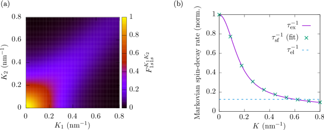
Figure 1: (Color online) (a) Angle-averaged form-factor product $F_{\eta_{\textrm{h}}1s1s}^{\eta_{\textrm{h}}K_{1}K_{2}}$ for the exciton ground state (1s) as a function of the center of mass momentum $K$. (b) $K$-dependence of the Markovian spin-decay rate for excitons ($\tau_{\textrm{ex}}^{-1}$), which follows the diagonal of plot (a), is compared to the constant rate found for quasi-free electronsCygorek et al. (2016a) ($\tau_{\textrm{el}}^{-1}$). Both rates are normalized with respect to the exciton spin-decay rate for $K=0$ and are calculated without external magnetic field. Additionally, Eq. (37) is used to fit $\tau_{\textrm{sf}}^{-1}$ to the exciton spin-decay rate of our model.

In the above equations, the shorthand notation $b^{\pm}:=\frac{1}{2}\big{(}\langle\mathbf{S}^{2}-(\mathbf{S}\cdot\mathbf{e}_{B})^{2}\rangle\pm\sigma_{S}^{B}\langle S^{\parallel}\rangle\big{)}$, $b^{\parallel}:=\frac{1}{2}\langle(\mathbf{S}\cdot\mathbf{e}_{B})^{2}\rangle$, and $b^{0}:=\sigma_{S}^{B}\langle S^{\parallel}\rangle$ has been used for the second moments of the Mn spin. Here, we model the optical excitation by the generation rates $\Gamma_{\mathbf{E}}^{\uparrow/\downarrow}$ and $\boldsymbol{\Gamma}_{\mathbf{E}}^{\perp}$ for the spin-up and spin-down occupations and the perpendicular spin component, respectively.

In Eq. (34), the term proportional to $\big{(}n_{xK}^{\uparrow/\downarrow}-n_{x_{1}K_{1}}^{\uparrow/\downarrow}\big{)}$ describes processes conserving the exciton spin, whereas the term proportional to $\big{(}b^{\pm}n_{xK}^{\downarrow/\uparrow}-b^{\mp}n_{x_{1}K_{1}}^{\uparrow/\downarrow}\big{)}$ is responsible for the spin-flip scattering of excitons. The delta functions ensure conservation of energy. Similarly, the terms proportional to $\big{(}\mathbf{s}_{xK}^{\perp}-\mathbf{s}_{x_{1}K_{1}}^{\perp}\big{)}$ in Eq. (34) can be interpreted as exciton-spin conserving contributions, whereas the prefactors of $s_{x_{1}K_{1}}^{\perp}$ are responsible for a decay of the perpendicular spin component. Finally, the cross product $\boldsymbol{\omega_{\textrm{e}}}\times\mathbf{s}^{\perp}_{x_{1}K_{1}}$ describes the mean-field precession around $\boldsymbol{\omega_{\textrm{e}}}$ which is renormalized by terms resulting from the imaginary part of the memory integral given by Eq. (31).

The exciton spin-conserving parts of Eqs. (34) lead to a redistribution within a given energy shell as well as to transitions between excitonic states with different quantum numbers, as can be seen from the argument of the corresponding delta functions. In situations where spin-orbit coupling and thus a D’yakonov-Perel’-type spin dephasing is important, these terms give rise to an additional momentum scattering and thereby indirectly influence the spin dynamics. However, spin-orbit coupling is typically of minor importance for the spin dynamics in DMS compared with the carrier-impurity interactionUngar et al. (2015). In an isotropic system as considered here, the exciton spin-conserving parts of Eqs. (34) do not influence the spin dynamics. Since the magnetic coupling constant $J_{pd}$ for the valence band as well as the non-magnetic coupling constants $J_{0}^{\textrm{e}}$ and $J_{0}^{\textrm{h}}$ only enter these terms, the nonmagnetic interactions and the $pd$ interaction do not affect the spin dynamics on the Markovian level.

For spin-flip scattering processes, an exciton with a given spin an energy $\hbar\omega_{x_{1}K_{1}}$ is scattered to a state with opposite spin and energy $\hbar\omega_{xK}$. The appearance of the energy shift $\pm\hbar(\sigma_{\textrm{e}}^{B}\omega_{\textrm{e}}-\sigma_{\textrm{Mn}}^{B}\omega_{\textrm{Mn}})$ in the corresponding delta function in Eq. (34) can be understood as follows: A flip of the exciton-bound electron spin requires or releases a magnetic energy $\hbar\sigma_{\textrm{e}}^{B}\omega_{\textrm{e}}$. But since a flip of a carrier spin also involves the flop of an impurity spin in the opposite direction, the corresponding change in magnetic energy of the impurity spin $\hbar\sigma_{\textrm{Mn}}^{B}\omega_{\textrm{Mn}}$ has to be accounted for to ensure conservation of energy.

An interesting limiting case can be worked out for zero external magnetic field, vanishing impurity magnetization, and optical excitation resonant with the $1s$ exciton state: Then, Eqs. (34) can be condensed into the simple rate equation

$$\frac{\partial}{\partial t}\mathbf{s}_{1sK_{1}} =-\tau^{-1}_{1sK_{1}}\mathbf{s}_{1sK_{1}},$$ (35)

where the spin-decay rate is given by

$$\tau^{-1}_{1sK_{1}} =\frac{35}{12}\frac{N_{\textrm{Mn}}IJ_{sd}^{2}M}{\hbar^{3}dV}F_{\eta_{\textrm{h}}1s1s}^{\eta_{\textrm{h}}K_{1}K_{1}}$$ (36)

and $d$ denotes the width of the DMS quantum well. In contrast to the quasi-free electron case, where the spin-decay rate is constant in a quantum wellKossut (1975); Wu et al. (2010), the decay rate for excitons explicitly depends on $K$, which is consistent with previous findings in the literatureBastard and Ferreira (1992).

III Results

We now apply our quantum kinetic theory to the exciton spin dynamics for vanishing external magnetic field and impurity magnetization after an ultrashort laser pulse resonant with the exciton ground state and compare the results with the corresponding Markovian calculations. In order to do so, it is necessary to first calculate the exciton wave functions and the resulting form-factor products $F_{\eta_{1}x_{1}K_{1}}^{\eta_{2}x_{2}K_{2}}$.

III.1 Exciton form factors

In order to calculate the exciton form factors, we first decompose the exciton wave function according to Eq. (19) and then numerically solve the Coulomb eigenvalue problem given by Eq. (16) for the radial part using a finite-difference method, which yields the exciton energies as well as the wave functions. From the exciton wave functions, the form-factor products defined in Eq. (II.5) are calculated. The steps and cut-offs in the real-space discretization have been adjusted to ensure convergence.

The results for the form-factor product $F_{\eta_{\textrm{h}}1s1s}^{\eta_{\textrm{h}}K_{1}K_{2}}$ relevant for spin-slip scattering on the $1s$ exciton parabola can be found in Fig. 1(a) as a function of wave numbers $K_{1}$ and $K_{2}$ using the parameters for Cd_1-xMn_xTe listed in Tab. 1. It can be seen that $F_{\eta_{\textrm{h}}1s1s}^{\eta_{\textrm{h}}K_{1}K_{2}}$ is symmetric with respect to the bisectrix and decreases continuously with increasing wave number. In Fig. 1(b), we present the spin-decay rate in the Markov limit according to Eq. (36) which follows the diagonal values $F_{\eta_{\textrm{h}}1s1s}^{\eta_{\textrm{h}}K_{1}K_{1}}$. To compare the resulting rate to the quasi-free electron case, we also plot the spin-decay rate from Ref. Cygorek et al., 2017 for electrons and normalize both results to the exciton spin-decay rate for $K=0$. The spin-decay rate for excitons at $K=0$ is about 8 times faster than the electron spin-decay rate, which is due to the much larger exciton mass. Furthermore, the exciton spin-decay rate strongly depends on $K$ and can even be smaller than the constant electron spin-decay rate for large wave numbers.

The fact that the spin-decay rate for excitons depends on $K$ has already been pointed out in Ref. Bastard and Ferreira, 1992. There, an exponential ansatz with a variational parameter for the radial part of the exciton wave function leads to the decay rateBastard and Ferreira (1992)

$$\frac{1}{\tau_{\textrm{sf}}}(K) =\frac{1}{\tau_{\textrm{sf}}}(0)\,\phi(\alpha^{2}K^{2}),$$ (37)

where the constant $\alpha$ contains the parameters of the model and the function $\phi$ is given byBastard and Ferreira (1992)

$$\phi(x) =\frac{1}{2}\big{(}1+(1+x)\big{)}\big{(}1+2x\big{)}^{-\frac{5}{2}}.$$ (38)

To compare this result to our calculations, we fit the constant $\alpha$ in Eq. (37) to our data obtained from Eq. (36) and plot the result in Fig. 1(b). It can be seen that the predictions of Ref. Bastard and Ferreira, 1992 agree with the Markovian limit of our quantum kinetic theory.

III.2 Spin dynamics

Having obtained the exciton form factors, we can now calculate the spin dynamics according to the quantum kinetic Eqs. (40). To address the question of the importance of quantum kinetic effects in the exciton spin dynamics, we also present numerical solutions of the Markovian Eqs. (34). Furthermore, we study the influence of nonmagnetic scattering as well as the magnetic $pd$ coupling.

For the numerical implementation, we use a forth-order Runge-Kutta algorithm to solve the differential equations in the time domain and discretize the $K$ space up to a cut-off energy of a few tens of meV. This is done in the quasi-continuous limit $\sum_{K}\to\int dKD^{2d}(K)$ using the two-dimensional density of states $D^{2d}(K)=\frac{A}{2\pi}K$ for a quantum well with area $A$. For all calculations, we have checked that the number of excitons in the system as well as the total energy remain constant after the pulse.

We limit our study to the exciton ground state and treat the optical excitation in a rotating-wave approximation. As discussed in section II.5, we focus on a situation where the hh spins are pinned and do not take part in the dynamics. Thus, our main quantity of interest is the time evolution of the spin of the exciton-bound electron. In all cases, the optical excitation is modeled by a circularly polarized Gaussian laser beam with a width (FWHM) of $100\,$fs centered at $t=0\,$ps resonant to the exciton ground state and we consider a quantum well with width $d=10\,$nm. We calculate the time evolution of the exciton spin for two different materials, namely Cd_1-xMn_xTe [Fig. 2(a)] as well as Zn_1-xMn_xSe [Fig. 2(b)] with impurity concentration $x=5\,\%$. The relevant parameters for these two materials, which are both of zinc blende crystal structureFurdyna (1988), are collected in Tab. 1.

parameter	Cd1-xMnxTe	Zn1-xMnxSe
$a\;(\textrm{nm})$Furdyna (1988)	$0.648$	$0.567$
$m_{\textrm{e}}/m_{0}$Astakhov et al. (2002); Triboulet and Siffert (2009)	$0.1$	$0.15$
$m_{\textrm{hh}}/m_{0}$Astakhov et al. (2002); Triboulet and Siffert (2009)	$0.7$	$0.8$
$J_{sd}\;(\textrm{meV}\,\textrm{nm}^{3})$Furdyna (1988)	$-15$	$-12$
$J_{pd}\;(\textrm{meV}\,\textrm{nm}^{3})$Furdyna (1988)	$60$	$50$
$J_{0}^{\textrm{e}}\;(\textrm{meV}\,\textrm{nm}^{3})$Furdyna (1988)	$110$	$22$
$J_{0}^{\textrm{h}}\;(\textrm{meV}\,\textrm{nm}^{3})$Furdyna (1988)	$7$	$0$
$\epsilon$Strzalkowski et al. (1976)	$10$	$9$

Table 1: Selected material parameters of Cd_1-xMn_xTe and Zn_1-xMn_xSe. The coupling constant is chosen such that it is consistent with the band offsets at a CdTe/Cd_1-xMn_xTe and ZnSe/Zn_1-xMn_xSe interface, respectivelyCygorek et al. (2017). The cubic lattice constant is given by $a$ and $m_{0}$ denotes the free electron mass.

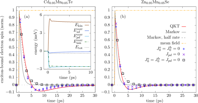
Figure 2: (Color online) Spin dynamics of the exciton-bound electron in a $10\,$nm quantum well using the parameters of (a) Cd_0.95Mn_0.05Te and (b) Zn_0.95Mn_0.05Se for vanishing external magnetic field after an optical excitation with a circularly polarized Gaussian laser beam resonant to the exciton ground state. The time axis is chosen such that the pulse maximum lies at $t=0\,$ps with a width (FWHM) of $100\,$fs. For each material, we show the quantum kinetic results based on Eqs. (40) (QKT) as well as Markovian calculations using Eqs. (34) (Markov), a spin decay with half the Markovian rate (Markov, half rate), and the results of a calculation where all correlations are neglected (mean field). Additionally, we plot the spin dynamics in the artificial situation where different coupling constants $J_{0}^{\textrm{e}}$, $J_{0}^{\textrm{h}}$ and/or $J_{pd}$ are set to zero. All results are normalized with respect to the mean-field spin polarization for long times. The inset in figure (a) shows the kinetic energy ($E_{\textrm{kin}}$), the magnetic $sd/pd$ correlation energies ($E_{sd/pd}^{\textrm{corr}}$), the nonmagnetic correlation energy ($E_{\textrm{nm}}^{\textrm{corr}}$), and the total energy ($E_{\textrm{tot}}$) normalized with respect to the exciton density after the pulse.

The mean-field results displayed in Fig. 2 show no spin decay because the time evolution of the exciton density matrix [c.f. Eq. (40)] after the optical excitation in the absence of a magnetic field is governed by the magnetic and nonmagnetic correlations, which are neglected in the mean-field approximation. If the correlations are treated on a Markovian level, the spin decays exponentially with the spin-decay rate $\tau_{1sK_{1}}^{-1}$ defined in Eq. (36). The spin dynamics in Cd_0.95Mn_0.05Te is slower than in Zn_0.95Mn_0.05Se, which is mainly due to the larger exciton mass in ZnSe.

However, the full quantum kinetic spin dynamics in both materials is clearly non-monotonic and shows a pronounced overshoot after approximately $5\,$ps of about $10\,\%$ of the spin polarization immediately after the pulse in the situation depicted in Fig. 2(a). Furthermore, for the first few picoseconds, the quantum kinetic result is actually closer to the results of a calculation using only half the Markovian spin-decay rate. The spin overshoot in Fig. 2 is absent if the nonmagnetic impurity scattering of electrons and holes in the DMS as well as the $pd$ exchange interaction are neglected, as suggested by a calculation with $J_{0}^{\textrm{e}}=J_{0}^{\textrm{h}}=J_{pd}=0$ (c.f. black boxes in Fig. 2). Without these contributions, the time evolution of the spin virtually coincides with an exponential decay with half the Markovian spin-decay rate. Note that the nonmagnetic scattering as well as the $pd$ interaction do not influence the spin dynamics on the Markovian level, as follows from Eqs. (34).

Interestingly, the role of non-magnetic impurity scattering is here opposite to what has been found for the electron spin dynamics in the band continuumCygorek et al. (2017): While for excitonic excitations this scattering enhances the overshoot, for above band-gap excitations it typically almost completely suppresses the non-monotonic time dependence of the electron spin polarization.

The deviations from the Markovian limit can be traced back to the optical excitation at the bottom of the exciton parabola ($K\approx 0$): While the memory kernel in the Markovian limit given by Eq. (31) contracts to a delta function in energy space, for finite times the energy-time uncertainty relation leads to a finite spectral width as sketched in Fig. 3. In a quantum well, the spectral density of states is constant but vanishes below the vertex of the exciton parabola, resulting in a cut-off of the memory kernel in energy spaceCygorek and Axt (2015). At $K=0$, the integral over the memory kernel yields therefore only half the value predicted by the Markovian assumption of a delta-like memory. This translates into a reduction of the effective spin-decay rate by a factor of $\frac{1}{2}$.

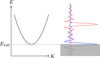
Figure 3: (Color online) Sketch of the $1s$ exciton parabola together with the real part of a typical memory kernel $\propto\frac{\sin[(E-E_{1})t/\hbar]}{(E-E_{1})/\hbar}$ [c.f. l.h.s. of Eq. (31)] for a fixed time $t$ with $E_{1}=E_{1s0}$ (blue solid line) and $E_{1}>E_{1s0}$ (red dashed line). For excitons optically generated at $K\approx 0$, the memory is effectively cut in half.

The influence of nonmagnetic impurity scattering manifests itself in a redistribution of center of mass momenta on the $1s$ exciton parabola. As a result, states further away from $K=0$ are populated. For these states, the cut-off of the memory integral due to the density of states is shifted correspondingly and oscillates with time, which causes the overshoots in the dynamics of the spin polarization in Fig. 2. It is noteworthy that, even if the heavy-hole spins are pinned throughout the dynamics, the magnetic $pd$ exchange interaction can still influence the dynamics of the exciton-bound electron spin since it allows for spin-conserving scattering of exciton-bound holes at magnetic impurities. In this sense, the magnetic $pd$ interaction has a similar effect as nonmagnetic scattering. This can be seen from the results depicted in Fig. 2 where either the nonmagnetic or the $pd$ interactions are switched off. In the case of Cd_0.95Mn_0.05Te, where $J_{pd}\approx\frac{1}{2}J_{0}^{\textrm{e}}$, both interactions are of similar importance. However, for Zn_0.95Mn_0.05Se, where $J_{pd}\approx 2J_{0}^{\textrm{e}}$, the magnetic $pd$ interaction dominates the spin dynamics and nonmagnetic impurity scattering is almost negligible.

The fact that the $pd$ interaction and the nonmagnetic impurity scattering facilitate a redistribution of center of mass momenta can be seen from the inset of Fig. 2(a), which shows the time evolution of the kinetic energy as well as correlation energies. A significant increase in kinetic energy of about $5\,$meV per exciton is found, which is mainly provided by a build-up of correlation energies due to nonmagnetic scattering and due to the $pd$ interaction. The inset in Fig. 2(a) also shows that the total exciton energy is indeed conserved after the pulse and obtains a small negative value with respect to the mean-field energy of a $1s$ exciton at $K=0$. This is possible because carrier-impurity correlations are built up already during the finite width of the pulse. In the case of Cd_0.95Mn_0.05Te the magnetic $pd$ interaction as well as the nonmagnetic impurity scattering lead to similar correlations energies, which is consistent with their comparable influence on the time evolution of the spin as depicted in the main panel of Fig. 2(a).

IV Conclusion

We have derived quantum kinetic equations for density matrices in the exciton representation that describe the time evolution of the exciton spin in laser-driven DMS in the presence of an external magnetic field. Our theory takes into account contributions up to second order in the generating laser field and explicitly keeps correlations between the carrier and the impurity subsystem. The model not only includes the magnetic $sp$-$d$ interaction between electrons, holes, and Mn atoms, but also accounts for elastic nonmagnetic scattering at the impurities. This makes our theory a widely applicable tool to study the ultrafast spin dynamics in DMS beyond the single-particle Born-Markov picture. Furthermore, we have shown how rate equations can be straightforwardly extracted from our quantum kinetic theory by using the Markov approximation to eliminate the correlations. This approach allows us to obtain spin-flip scattering rates for situations where the spin polarization is oriented parallel or perpendicular with respect to the external magnetic field. In contrast to the situation of quasi-free conduction band electrons studied in Ref. Cygorek et al., 2017, for excitons it is found that the Markovian spin-decay rate strongly depends on the wave vector via a form factor reflecting the shape of the exciton wave function.

A numerical solution of the quantum kinetic equations including exciton-impurity correlations in the absence of a magnetic field and for vanishing impurity magnetization reveals strong deviations from the Markovian predictions in the form of an overshoot of the spin polarization as well as a slower initial decay with about half of the Markovian rate. Accounting for nonmagnetic impurity interaction as well as the $pd$ interaction in the valence band was found to have an essential impact on the spin polarization since the overshoot is only seen in calculations that include these interactions. In contrast, non-monotonic behavior in the spin dynamics of conduction band electrons is strongly suppressed by nonmagnetic impurity scatteringCygorek et al. (2017).

In Ref. Ben Cheikh et al., 2013, where results for spin-decay rates in DMS measured by different groups have been compared, it was found that the experimentally obtained rates for vanishing magnetic field are consistently about a factor of $5$ larger than the value expected from Fermi’s golden rule for conduction band electrons. A possible explanation for this deviation is that excitons instead of quasi-free electrons have to be considered. Substituting the exciton mass for the electron mass in Fermi’s golden rule leads to an approximately 8 times larger spin-decay rate. However, in this article, we have found that non-Markovian effects lead to a spin decay on a time scale corresponding to about half the Markovian rate. Thus, our theory predicts that the spin-decay rate measurable in ultrafast optical experiments is about 4 times larger than predicted by a Markovian model using quasi-free carriers and is therefore close to the findings of experiments.

Appendix A Source terms for the correlations

The source terms for the correlations in Eqs. (25) are:

$${\beta_{n_{1}x_{1}\mathbf{K}_{1}}^{n_{2}v_{1}l_{1}}(z)}^{I}=\sum_{nx}M_{n_{1}n}(z)\mathbf{S}_{n_{2}n}\cdot\Big{(}J_{sd}d|u_{0}^{\textrm{e}}(z)|^{2}\sum_{l}\mathbf{s}^{\textrm{e}}_{l_{1}l}f_{-\eta_{\textrm{h}}x_{1}x}^{\phantom{-\eta_{\textrm{h}}}\mathbf{K}_{1}\mathbf{0}}Y_{x\mathbf{0}}^{v_{1}l}+J_{pd}d|u_{0}^{\textrm{h}}(z)|^{2}\sum_{v}\mathbf{s}^{\textrm{h}}_{v_{1}v}f_{\eta_{\textrm{e}}x_{1}x}^{\phantom{\eta_{\textrm{e}}}\mathbf{K}_{1}\mathbf{0}}Y_{x\mathbf{0}}^{vl_{1}}\Big{)}$$

$$\phantom{{\beta_{n_{1}x_{1}\mathbf{K}_{1}}^{n_{2}v_{1}l_{1}}(z)}^{I}=\,}+\sum_{x}M_{n_{1}}^{n_{2}}(z)\Big{(}J_{0}^{\textrm{e}}d|u_{0}^{\textrm{e}}(z)|^{2}f_{-\eta_{\textrm{h}}x_{1}x}^{\phantom{-\eta_{\textrm{h}}}\mathbf{K}_{1}\mathbf{0}}+J_{0}^{\textrm{h}}d|u_{0}^{\textrm{h}}(z)|^{2}f_{\eta_{\textrm{e}}x_{1}x}^{\phantom{\eta_{\textrm{e}}}\mathbf{K}_{1}\mathbf{0}}\Big{)}Y_{x\mathbf{0}}^{v_{1}l_{1}},\allowdisplaybreaks$$ (39a)

$${\beta_{n_{1}x_{1}\mathbf{K}_{1}}^{n_{2}v_{1}l_{1}}(z)}^{II}=\sum_{l}\hbar\boldsymbol{\omega_{\textrm{e}}}\cdot\mathbf{s}^{\textrm{e}}_{l_{1}l}{Q_{Y}}_{n_{1}x_{1}\mathbf{K}_{1}}^{n_{2}v_{1}l}(z)+\sum_{v}\hbar\boldsymbol{\omega_{\textrm{h}}}\cdot\mathbf{s}^{\textrm{h}}_{v_{1}v}{Q_{Y}}_{n_{1}x_{1}\mathbf{K}_{1}}^{n_{2}vl_{1}}(z)$$

$$\phantom{{\beta_{n_{1}x_{1}\mathbf{K}_{1}}^{n_{2}v_{1}l_{1}}(z)}^{II}=\,}+\sum_{n}\hbar\boldsymbol{\omega_{\textrm{Mn}}}\cdot\Big{(}\mathbf{S}_{n_{2}n}{Q_{Y}}_{n_{1}x_{1}\mathbf{K}_{1}}^{nv_{1}l_{1}}(z)-\mathbf{S}_{nn_{1}}{Q_{Y}}_{nx_{1}\mathbf{K}_{1}}^{n_{2}v_{1}l_{1}}(z)\Big{)},\allowdisplaybreaks$$ (39b)

$${\beta_{n_{1}x_{1}\mathbf{K}_{1}}^{n_{2}v_{1}l_{1}}(z)}^{III}=\frac{1}{V}\sum_{nx\mathbf{K}}\mathbf{S}_{n_{2}n}\cdot\Big{(}J_{sd}d|u_{0}^{\textrm{e}}(z)|^{2}\sum_{l}\mathbf{s}^{\textrm{e}}_{l_{1}l}f_{-\eta_{\textrm{h}}x_{1}x}^{\phantom{-\eta_{\textrm{h}}}\mathbf{K}_{1}\mathbf{K}}{Q_{Y}}_{n_{1}x\mathbf{K}}^{nv_{1}l}(z)+J_{pd}d|u_{0}^{\textrm{h}}(z)|^{2}\sum_{v}\mathbf{s}^{\textrm{h}}_{v_{1}v}f_{\eta_{\textrm{e}}x_{1}x}^{\phantom{\eta_{\textrm{e}}}\mathbf{K}_{1}\mathbf{K}}{Q_{Y}}_{n_{1}x\mathbf{K}}^{nvl_{1}}(z)\Big{)}$$

$$\phantom{{\beta_{n_{1}x_{1}\mathbf{K}_{1}}^{n_{2}v_{1}l_{1}}(z)}^{III}=\,}+\frac{1}{V}\sum_{x\mathbf{K}}\Big{(}J_{0}^{\textrm{e}}d|u_{0}^{\textrm{e}}(z)|^{2}f_{-\eta_{\textrm{h}}x_{1}x}^{\phantom{-\eta_{\textrm{h}}}\mathbf{K}_{1}\mathbf{K}}+J_{0}^{\textrm{h}}d|u_{0}^{\textrm{h}}(z)|^{2}f_{\eta_{\textrm{e}}x_{1}x}^{\phantom{\eta_{\textrm{e}}}\mathbf{K}_{1}\mathbf{K}}\Big{)}{Q_{Y}}_{n_{1}x\mathbf{K}}^{n_{2}v_{1}l_{1}}(z),\allowdisplaybreaks$$ (39c)

$${\bar{\beta}_{x_{1}\mathbf{K}_{1}}^{v_{1}l_{1}}(z)}^{I}=\sum_{nn^{\prime}x}M_{n}^{n^{\prime}}(z)\mathbf{S}_{nn^{\prime}}\cdot\Big{(}J_{sd}d|u_{0}^{\textrm{e}}(z)|^{2}\sum_{l}\mathbf{s}^{\textrm{e}}_{l_{1}l}f_{-\eta_{\textrm{h}}x_{1}x}^{\phantom{-\eta_{\textrm{h}}}\mathbf{K}_{1}\mathbf{0}}Y_{x\mathbf{0}}^{v_{1}l}+J_{pd}d|u_{0}^{\textrm{h}}(z)|^{2}\sum_{v}\mathbf{s}^{\textrm{h}}_{v_{1}v}f_{\eta_{\textrm{e}}x_{1}x}^{\phantom{\eta_{\textrm{e}}}\mathbf{K}_{1}\mathbf{0}}Y_{x\mathbf{0}}^{vl_{1}}\Big{)}$$

$$\phantom{{\bar{\beta}_{x_{1}\mathbf{K}_{1}}^{v_{1}l_{1}}(z)}^{I}=\,}+\sum_{x}\Big{(}J_{0}^{\textrm{e}}d|u_{0}^{\textrm{e}}(z)|^{2}f_{-\eta_{\textrm{h}}x_{1}x}^{\phantom{-\eta_{\textrm{h}}}\mathbf{K}_{1}\mathbf{0}}+J_{0}^{\textrm{h}}d|u_{0}^{\textrm{h}}(z)|^{2}f_{\eta_{\textrm{e}}x_{1}x}^{\phantom{\eta_{\textrm{e}}}\mathbf{K}_{1}\mathbf{0}}\Big{)}Y_{x\mathbf{0}}^{v_{1}l_{1}},\allowdisplaybreaks$$ (39d)

$${\bar{\beta}_{x_{1}\mathbf{K}_{1}}^{v_{1}l_{1}}(z)}^{II}=\sum_{l}\hbar\boldsymbol{\omega_{\textrm{e}}}\cdot\mathbf{s}^{\textrm{e}}_{l_{1}l}\bar{Y}_{x_{1}\mathbf{K}_{1}}^{v_{1}l}(z)+\sum_{v}\hbar\boldsymbol{\omega_{\textrm{h}}}\cdot\mathbf{s}^{\textrm{h}}_{v_{1}v}\bar{Y}_{x_{1}\mathbf{K}_{1}}^{vl_{1}}(z),\allowdisplaybreaks$$ (39e)

$${\bar{\beta}_{x_{1}\mathbf{K}_{1}}^{v_{1}l_{1}}(z)}^{III}=\frac{1}{V}\sum_{\begin{subarray}{c}nn^{\prime}\\ x\mathbf{K}\end{subarray}}\mathbf{S}_{nn^{\prime}}\cdot\Big{(}J_{sd}d|u_{0}^{\textrm{e}}(z)|^{2}\sum_{l}\mathbf{s}^{\textrm{e}}_{l_{1}l}f_{-\eta_{\textrm{h}}x_{1}x}^{\phantom{-\eta_{\textrm{h}}}\mathbf{K}_{1}\mathbf{K}}{Q_{Y}}_{nx\mathbf{K}}^{n^{\prime}v_{1}l}(z)+J_{pd}d|u_{0}^{\textrm{h}}(z)|^{2}\sum_{v}\mathbf{s}^{\textrm{h}}_{v_{1}v}f_{\eta_{\textrm{e}}x_{1}x}^{\phantom{\eta_{\textrm{e}}}\mathbf{K}_{1}\mathbf{K}}{Q_{Y}}_{nx\mathbf{K}}^{n^{\prime}vl_{1}}(z)\Big{)}$$

$$\phantom{{\bar{\beta}_{x_{1}\mathbf{K}_{1}}^{v_{1}l_{1}}(z)}^{III}=\,}+\frac{1}{V}\sum_{x\mathbf{K}}\Big{(}J_{0}^{\textrm{e}}d|u_{0}^{\textrm{e}}(z)|^{2}f_{-\eta_{\textrm{h}}x_{1}x}^{\phantom{-\eta_{\textrm{h}}}\mathbf{K}_{1}\mathbf{K}}+J_{0}^{\textrm{h}}d|u_{0}^{\textrm{h}}(z)|^{2}f_{\eta_{\textrm{e}}x_{1}x}^{\phantom{\eta_{\textrm{e}}}\mathbf{K}_{1}\mathbf{K}}\Big{)}\bar{Y}_{x\mathbf{K}}^{v_{1}l_{1}}(z),\allowdisplaybreaks$$ (39f)

$${b_{n_{1}x_{1}\mathbf{K}_{1}x_{2}\mathbf{K}_{2}}^{n_{2}l_{1}v_{1}v_{2}l_{2}}(z)}^{I}=J_{sd}d|u_{0}^{\textrm{e}}(z)|^{2}\sum_{ln}f_{-\eta_{\textrm{h}}x_{2}x_{1}}^{\phantom{-\eta_{\textrm{h}}}\mathbf{K}_{2}\mathbf{K}_{1}}\Big{(}\mathbf{S}_{n_{2}n}M_{n_{1}}^{n}(z)\cdot\mathbf{s}^{\textrm{e}}_{l_{2}l}N_{x_{1}\mathbf{K}_{1}}^{l_{1}v_{1}v_{2}l}-\mathbf{S}_{nn_{1}}M_{n}^{n_{2}}(z)\cdot\mathbf{s}^{\textrm{e}}_{ll_{1}}N_{x_{2}\mathbf{K}_{2}}^{lv_{1}v_{2}l_{2}}\Big{)}$$

$$\phantom{{b_{n_{1}x_{1}\mathbf{K}_{1}x_{2}\mathbf{K}_{2}}^{n_{2}l_{1}v_{1}v_{2}l_{2}}(z)}^{I}=\,}+J_{pd}d|u_{0}^{\textrm{h}}(z)|^{2}\sum_{vn}f_{\eta_{\textrm{e}}x_{2}x_{1}}^{\phantom{\eta_{\textrm{e}}}\mathbf{K}_{2}\mathbf{K}_{1}}\Big{(}\mathbf{S}_{n_{2}n}M_{n_{1}}^{n}(z)\cdot\mathbf{s}^{\textrm{h}}_{v_{2}v}N_{x_{1}\mathbf{K}_{1}}^{l_{1}v_{1}vl_{2}}-\mathbf{S}_{nn_{1}}M_{n}^{n_{2}}(z)\cdot\mathbf{s}^{\textrm{h}}_{vv_{1}}N_{x_{2}\mathbf{K}_{2}}^{l_{1}vv_{2}l_{2}}\Big{)}$$

$$\phantom{{b_{n_{1}x_{1}\mathbf{K}_{1}x_{2}\mathbf{K}_{2}}^{n_{2}l_{1}v_{1}v_{2}l_{2}}(z)}^{I}=\,}+M_{n_{1}}^{n_{2}}(z)\Big{(}J_{0}^{\textrm{e}}d|u_{0}^{\textrm{e}}(z)|^{2}f_{-\eta_{\textrm{h}}x_{2}x_{1}}^{\phantom{-\eta_{\textrm{h}}}\mathbf{K}_{2}\mathbf{K}_{1}}+J_{0}^{\textrm{h}}d|u_{0}^{\textrm{h}}(z)|^{2}f_{\eta_{\textrm{e}}x_{2}x_{1}}^{\phantom{\eta_{\textrm{e}}}\mathbf{K}_{2}\mathbf{K}_{1}}\Big{)}\Big{(}N_{x_{1}\mathbf{K}_{1}}^{l_{1}v_{1}v_{2}l_{2}}-N_{x_{2}\mathbf{K}_{2}}^{l_{1}v_{1}v_{2}l_{2}}\Big{)},\allowdisplaybreaks$$ (39g)

$${b_{n_{1}x_{1}\mathbf{K}_{1}x_{2}\mathbf{K}_{2}}^{n_{2}l_{1}v_{1}v_{2}l_{2}}(z)}^{II}=\sum_{l}\hbar\boldsymbol{\omega_{\textrm{e}}}\cdot\Big{(}\mathbf{s}^{\textrm{e}}_{l_{2}l}{Q_{N}}_{n_{1}x_{1}\mathbf{K}_{1}x_{2}\mathbf{K}_{2}}^{n_{2}l_{1}v_{1}v_{2}l}(z)-\mathbf{s}^{\textrm{e}}_{ll_{1}}{Q_{N}}_{n_{1}x_{1}\mathbf{K}_{1}x_{2}\mathbf{K}_{2}}^{n_{2}lv_{1}v_{2}l_{2}}(z)\Big{)}$$

$$\phantom{{b_{n_{1}x_{1}\mathbf{K}_{1}x_{2}\mathbf{K}_{2}}^{n_{2}l_{1}v_{1}v_{2}l_{2}}(z)}^{II}=\,}+\sum_{v}\hbar\boldsymbol{\omega_{\textrm{h}}}\cdot\Big{(}\mathbf{s}^{\textrm{h}}_{v_{2}v}{Q_{N}}_{n_{1}x_{1}\mathbf{K}_{1}x_{2}\mathbf{K}_{2}}^{n_{2}l_{1}v_{1}vl_{2}}(z)-\mathbf{s}^{\textrm{h}}_{vv_{1}}{Q_{N}}_{n_{1}x_{1}\mathbf{K}_{1}x_{2}\mathbf{K}_{2}}^{n_{2}l_{1}vv_{2}l_{2}}(z)\Big{)}$$

$$\phantom{{b_{n_{1}x_{1}\mathbf{K}_{1}x_{2}\mathbf{K}_{2}}^{n_{2}l_{1}v_{1}v_{2}l_{2}}(z)}^{II}=\,}+\sum_{n}\hbar\boldsymbol{\omega_{\textrm{Mn}}}\cdot\Big{(}\mathbf{S}_{n_{2}n}{Q_{N}}_{n_{1}x_{1}\mathbf{K}_{1}x_{2}\mathbf{K}_{2}}^{nl_{1}v_{1}v_{2}l_{2}}(z)-\mathbf{S}_{nn_{1}}{Q_{N}}_{nx_{1}\mathbf{K}_{1}x_{2}\mathbf{K}_{2}}^{n_{2}l_{1}v_{1}v_{2}l_{2}}(z)\Big{)},\allowdisplaybreaks$$ (39h)

$${b_{n_{1}x_{1}\mathbf{K}_{1}x_{2}\mathbf{K}_{2}}^{n_{2}l_{1}v_{1}v_{2}l_{2}}(z)}^{III}=\frac{J_{sd}}{V}d|u_{0}^{\textrm{e}}(z)|^{2}\sum_{\begin{subarray}{c}ln\\ x\mathbf{K}\end{subarray}}\Big{(}\mathbf{S}_{n_{2}n}\cdot\mathbf{s}^{\textrm{e}}_{l_{2}l}f_{-\eta_{\textrm{h}}x_{2}x}^{\phantom{-\eta_{\textrm{h}}}\mathbf{K}_{2}\mathbf{K}}{Q_{N}}_{n_{1}x_{1}\mathbf{K}_{1}x\mathbf{K}}^{nl_{1}v_{1}v_{2}l}(z)-\mathbf{S}_{nn_{1}}\cdot\mathbf{s}^{\textrm{e}}_{ll_{1}}f_{-\eta_{\textrm{h}}xx_{1}}^{\phantom{-\eta_{\textrm{h}}}\mathbf{K}\mathbf{K}_{1}}{Q_{N}}_{nx\mathbf{K}x_{2}\mathbf{K}_{2}}^{n_{2}lv_{1}v_{2}l_{2}}(z)\Big{)}$$

$$\phantom{{b_{n_{1}x_{1}\mathbf{K}_{1}x_{2}\mathbf{K}_{2}}^{n_{2}l_{1}v_{1}v_{2}l_{2}}(z)}^{III}=\,}+\frac{J_{pd}}{V}d|u_{0}^{\textrm{h}}(z)|^{2}\sum_{\begin{subarray}{c}vn\\ x\mathbf{K}\end{subarray}}\Big{(}\mathbf{S}_{n_{2}n}\cdot\mathbf{s}^{\textrm{h}}_{v_{3}v}f_{\eta_{\textrm{e}}x_{2}x}^{(-\eta_{\textrm{e}})\mathbf{K}_{2}\mathbf{K}}{Q_{N}}_{n_{1}x_{1}\mathbf{K}_{1}x\mathbf{K}}^{nl_{1}v_{1}vl_{2}}(z)-\mathbf{S}_{nn_{1}}\cdot\mathbf{s}^{\textrm{h}}_{vv_{2}}f_{\eta_{\textrm{e}}xx_{1}}^{\phantom{\eta_{\textrm{e}}}\mathbf{K}\mathbf{K}_{1}}{Q_{N}}_{nx\mathbf{K}x_{2}\mathbf{K}_{2}}^{n_{2}l_{1}vv_{2}l_{2}}(z)\Big{)}$$

$$\phantom{{b_{n_{1}x_{1}\mathbf{K}_{1}x_{2}\mathbf{K}_{2}}^{n_{2}l_{1}v_{1}v_{2}l_{2}}(z)}^{III}=\,}+\frac{J_{0}^{\textrm{e}}}{V}\sum_{x\mathbf{K}}d|u_{0}^{\textrm{e}}(z)|^{2}\Big{(}f_{-\eta_{\textrm{h}}x_{2}x}^{\phantom{-\eta_{\textrm{h}}}\mathbf{K}_{2}\mathbf{K}}{Q_{N}}_{n_{1}x_{1}\mathbf{K}_{1}x\mathbf{K}}^{n_{2}l_{1}v_{1}v_{2}l_{2}}(z)-f_{-\eta_{\textrm{h}}xx_{1}}^{\phantom{-\eta_{\textrm{h}}}\mathbf{K}\mathbf{K}_{1}}{Q_{N}}_{n_{1}x\mathbf{K}x_{2}\mathbf{K}_{2}}^{n_{2}l_{1}v_{1}v_{2}l_{2}}(z)\Big{)}$$

$$\phantom{{b_{n_{1}x_{1}\mathbf{K}_{1}x_{2}\mathbf{K}_{2}}^{n_{2}l_{1}v_{1}v_{2}l_{2}}(z)}^{III}=\,}+\frac{J_{0}^{\textrm{h}}}{V}\sum_{x\mathbf{K}}d|u_{0}^{\textrm{h}}(z)|^{2}\Big{(}f_{\eta_{\textrm{e}}x_{2}x}^{\phantom{\eta_{\textrm{e}}}\mathbf{K}_{2}\mathbf{K}}{Q_{N}}_{n_{1}x_{1}\mathbf{K}_{1}x\mathbf{K}}^{n_{2}l_{1}v_{1}v_{2}l_{2}}(z)-f_{\eta_{\textrm{e}}xx_{1}}^{\phantom{\eta_{\textrm{e}}}\mathbf{K}\mathbf{K}_{1}}{Q_{N}}_{n_{1}x\mathbf{K}x_{2}\mathbf{K}_{2}}^{n_{2}l_{1}v_{1}v_{2}l_{2}}(z)\Big{)},\allowdisplaybreaks$$ (39i)

$${\bar{b}_{x_{1}\mathbf{K}_{1}x_{2}\mathbf{K}_{2}}^{l_{1}v_{1}v_{2}l_{2}}(z)}^{I}=\frac{J_{sd}N_{\textrm{Mn}}}{V}d|u_{0}^{\textrm{e}}(z)|^{2}\sum_{lnn^{\prime}}\mathbf{S}_{nn^{\prime}}M_{n}^{n^{\prime}}(z)\cdot f_{-\eta_{\textrm{h}}x_{2}x_{1}}^{\phantom{-\eta_{\textrm{h}}}\mathbf{K}_{2}\mathbf{K}_{1}}\Big{(}\mathbf{s}^{\textrm{e}}_{l_{2}l}N_{x_{1}\mathbf{K}_{1}}^{l_{1}v_{1}v_{2}l}-\mathbf{s}^{\textrm{e}}_{ll_{1}}N_{x_{2}\mathbf{K}_{2}}^{lv_{1}v_{2}l_{2}}\Big{)}$$

$$\phantom{{\bar{b}_{x_{1}\mathbf{K}_{1}x_{2}\mathbf{K}_{2}}^{l_{1}v_{1}v_{2}l_{2}}(z)}^{I}=\,}+\frac{J_{pd}N_{\textrm{Mn}}}{V}d|u_{0}^{\textrm{h}}(z)|^{2}\sum_{vnn^{\prime}}\mathbf{S}_{nn^{\prime}}M_{n}^{n^{\prime}}(z)\cdot f_{\eta_{\textrm{e}}x_{2}x_{1}}^{\phantom{\eta_{\textrm{e}}}\mathbf{K}_{2}\mathbf{K}_{1}}\Big{(}\mathbf{s}^{\textrm{h}}_{v_{2}v}N_{x_{1}\mathbf{K}_{1}}^{l_{1}v_{1}vl_{2}}-\mathbf{s}^{\textrm{h}}_{vv_{1}}N_{x_{2}\mathbf{K}_{2}}^{l_{1}vv_{2}l_{2}}\Big{)}$$

$$\phantom{{\bar{b}_{x_{1}\mathbf{K}_{1}x_{2}\mathbf{K}_{2}}^{l_{1}v_{1}v_{2}l_{2}}(z)}^{I}=\,}+\Big{(}J_{0}^{\textrm{e}}d|u_{0}^{\textrm{e}}(z)|^{2}f_{-\eta_{\textrm{h}}x_{2}x_{1}}^{\phantom{-\eta_{\textrm{h}}}\mathbf{K}_{2}\mathbf{K}_{1}}+J_{0}^{\textrm{h}}d|u_{0}^{\textrm{h}}(z)|^{2}f_{\eta_{\textrm{e}}x_{2}x_{1}}^{\phantom{\eta_{\textrm{e}}}\mathbf{K}_{2}\mathbf{K}_{1}}\Big{)}\Big{(}N_{x_{1}\mathbf{K}_{1}}^{l_{1}v_{1}v_{2}l_{2}}-N_{x_{2}\mathbf{K}_{2}}^{l_{1}v_{1}v_{2}l_{2}}\Big{)},\allowdisplaybreaks$$ (39j)

$${\bar{b}_{x_{1}\mathbf{K}_{1}x_{2}\mathbf{K}_{2}}^{l_{1}v_{1}v_{2}l_{2}}(z)}^{II}=\sum_{l}\hbar\boldsymbol{\omega_{\textrm{e}}}\cdot\Big{(}\mathbf{s}^{\textrm{e}}_{l_{2}l}\bar{N}_{x_{1}\mathbf{K}_{1}x_{2}\mathbf{K}_{2}}^{l_{1}v_{1}v_{2}l}(z)-\mathbf{s}^{\textrm{e}}_{ll_{1}}\bar{N}_{x_{1}\mathbf{K}_{1}x_{2}\mathbf{K}_{2}}^{lv_{1}v_{2}l_{2}}(z)\Big{)}$$

$$\phantom{{\bar{b}_{x_{1}\mathbf{K}_{1}x_{2}\mathbf{K}_{2}}^{l_{1}v_{1}v_{2}l_{2}}(z)}^{II}=\,}+\sum_{v}\hbar\boldsymbol{\omega_{\textrm{h}}}\cdot\Big{(}\mathbf{s}^{\textrm{h}}_{v_{2}v}\bar{N}_{x_{1}\mathbf{K}_{1}x_{2}\mathbf{K}_{2}}^{l_{1}v_{1}vl_{2}}(z)-\mathbf{s}^{\textrm{h}}_{vv_{1}}\bar{N}_{x_{1}\mathbf{K}_{1}x_{2}\mathbf{K}_{2}}^{l_{1}vv_{2}l_{2}}(z)\Big{)},\allowdisplaybreaks$$ (39k)

$${\bar{b}_{x_{1}\mathbf{K}_{1}x_{2}\mathbf{K}_{2}}^{l_{1}v_{1}v_{2}l_{2}}(z)}^{III}=\frac{J_{sd}N_{\textrm{Mn}}}{V^{2}}d|u_{0}^{\textrm{e}}(z)|^{2}\sum_{\begin{subarray}{c}lnn^{\prime}\\ x\mathbf{K}\end{subarray}}\mathbf{S}_{nn^{\prime}}\cdot\Big{(}\mathbf{s}^{\textrm{e}}_{l_{2}l}f_{-\eta_{\textrm{h}}x_{2}x}^{\phantom{-\eta_{\textrm{h}}}\mathbf{K}_{2}\mathbf{K}}{Q_{N}}_{n_{1}x_{1}\mathbf{K}_{1}x\mathbf{K}}^{nl_{1}v_{1}v_{2}l}(z)-\mathbf{s}^{\textrm{e}}_{ll_{1}}f_{-\eta_{\textrm{h}}xx_{1}}^{\phantom{-\eta_{\textrm{h}}}\mathbf{K}\mathbf{K}_{1}}{Q_{N}}_{nx\mathbf{K}x_{2}\mathbf{K}_{2}}^{n_{2}lv_{1}v_{2}l_{2}}(z)\Big{)}$$

$$\phantom{{\bar{b}_{x_{1}\mathbf{K}_{1}x_{2}\mathbf{K}_{2}}^{l_{1}v_{1}v_{2}l_{2}}(z)}^{III}=\,}+\frac{J_{pd}N_{\textrm{Mn}}}{V^{2}}d|u_{0}^{\textrm{h}}(z)|^{2}\sum_{\begin{subarray}{c}vnn^{\prime}\\ x\mathbf{K}\end{subarray}}\mathbf{S}_{nn^{\prime}}\cdot\Big{(}\mathbf{s}^{\textrm{h}}_{v_{2}v}f_{\eta_{\textrm{e}}x_{2}x}^{\phantom{\eta_{\textrm{e}}}\mathbf{K}_{2}\mathbf{K}}{Q_{N}}_{n_{1}x_{1}\mathbf{K}_{1}x\mathbf{K}}^{nl_{1}v_{1}vl_{2}}(z)-\mathbf{s}^{\textrm{h}}_{vv_{1}}f_{\eta_{\textrm{e}}xx_{1}}^{\phantom{\eta_{\textrm{e}}}\mathbf{K}\mathbf{K}_{1}}{Q_{N}}_{nx\mathbf{K}x_{2}\mathbf{K}_{2}}^{n_{2}l_{1}vv_{2}l_{2}}(z)\Big{)}$$

$$\phantom{{\bar{b}_{x_{1}\mathbf{K}_{1}x_{2}\mathbf{K}_{2}}^{l_{1}v_{1}v_{2}l_{2}}(z)}^{III}=\,}+\frac{J_{0}^{\textrm{e}}}{V}d|u_{0}^{\textrm{e}}(z)|^{2}\sum_{x\mathbf{K}}\Big{(}f_{-\eta_{\textrm{h}}x_{2}x}^{\phantom{-\eta_{\textrm{h}}}\mathbf{K}_{2}\mathbf{K}}\bar{N}_{x_{1}\mathbf{K}_{1}x\mathbf{K}}^{l_{1}v_{1}v_{2}l_{2}}(z)-f_{-\eta_{\textrm{h}}xx_{1}}^{\phantom{-\eta_{\textrm{h}}}\mathbf{K}\mathbf{K}_{1}}\bar{N}_{x\mathbf{K}x_{2}\mathbf{K}_{2}}^{l_{1}v_{1}v_{2}l_{2}}(z)\Big{)}$$

$$\phantom{{\bar{b}_{x_{1}\mathbf{K}_{1}x_{2}\mathbf{K}_{2}}^{l_{1}v_{1}v_{2}l_{2}}(z)}^{III}=\,}+\frac{J_{0}^{\textrm{h}}}{V}d|u_{0}^{\textrm{h}}(z)|^{2}\sum_{x\mathbf{K}}\Big{(}f_{\eta_{\textrm{e}}x_{2}x}^{\phantom{\eta_{\textrm{e}}}\mathbf{K}_{2}\mathbf{K}}\bar{N}_{x_{1}\mathbf{K}_{1}x\mathbf{K}}^{l_{1}v_{1}v_{2}l_{2}}(z)-f_{\eta_{\textrm{e}}xx_{1}}^{\phantom{\eta_{\textrm{e}}}\mathbf{K}\mathbf{K}_{1}}\bar{N}_{x\mathbf{K}x_{2}\mathbf{K}_{2}}^{l_{1}v_{1}v_{2}l_{2}}(z)\Big{)}.$$ (39l)

Appendix B Quantum kinetic equations of motion with pinned hole spin

In this section, we provide the equations of motion corresponding to the variables defined in Eqs. (28) after performing an angle-averaging in $\mathbf{K}$ space. Using the Einstein summation convention, the equations read:

$$\frac{\partial}{\partial t}n_{x_{1}K_{1}} =\frac{1}{\hbar}\mathbf{E}\cdot\mathbf{M}2\textrm{Im}\big{[}y_{x_{1}}^{\uparrow}\phi_{x_{1}}\big{]}\delta_{K_{1},0}-\frac{J_{sd}N_{\textrm{Mn}}}{\hbar V^{2}}\sum_{xK}2\textrm{Im}\big{[}Q_{-\eta_{\textrm{h}}ixK}^{\phantom{-\eta_{\textrm{h}}}ix_{1}K_{1}}\big{]}+\frac{J_{pd}N_{\textrm{Mn}}}{\hbar V^{2}}\sum_{xK}\textrm{Im}\big{[}Q_{\eta_{\textrm{e}}zxK}^{\phantom{\eta_{\textrm{e}}}0x_{1}K_{1}}\big{]}$$

$$\phantom{=\;}-\frac{J_{0}^{\textrm{e}}N_{\textrm{Mn}}}{\hbar V^{2}}\sum_{xK}2\textrm{Im}\big{[}Z_{-\eta_{\textrm{h}}\phantom{0}xK}^{\phantom{-\eta_{\textrm{h}}}0x_{1}K_{1}}\big{]}-\frac{J_{0}^{\textrm{h}}N_{\textrm{Mn}}}{\hbar V^{2}}\sum_{xK}2\textrm{Im}\big{[}Z_{\eta_{\textrm{e}}\phantom{0}xK}^{\phantom{\eta_{\textrm{e}}}0x_{1}K_{1}}\big{]},\allowdisplaybreaks$$ (40a)

$$\frac{\partial}{\partial t}s_{x_{1}K_{1}}^{l} =\frac{1}{\hbar}\mathbf{E}\cdot\mathbf{M}\Big{(}\textrm{Im}\big{[}y_{x_{1}}^{\uparrow}\phi_{x_{1}}\big{]}\delta_{K_{1},0}\delta_{l,z}+\textrm{Im}\big{[}y_{x_{1}}^{\downarrow}\phi_{x_{1}}\big{]}\delta_{K_{1},0}\delta_{l,x}-\textrm{Re}\big{[}y_{x_{1}}^{\downarrow}\phi_{x_{1}}\big{]}\delta_{K_{1},0}\delta_{l,y}\Big{)}+\epsilon_{ijl}\omega_{\textrm{e}}^{i}s_{x_{1}K_{1}}^{j}$$

$$\phantom{=\;}+\frac{J_{sd}N_{\textrm{Mn}}}{\hbar V^{2}}\sum_{xK}\Big{(}\epsilon_{ijl}\textrm{Re}\big{[}Q_{-\eta_{\textrm{h}}ixK}^{\phantom{-\eta_{\textrm{h}}}jx_{1}K_{1}}\big{]}-\frac{1}{2}\textrm{Im}\big{[}Q_{-\eta_{\textrm{h}}lxK}^{\phantom{-\eta_{\textrm{h}}}0x_{1}K_{1}}\big{]}\Big{)}+\frac{J_{pd}N_{\textrm{Mn}}}{\hbar V^{2}}\sum_{xK}\textrm{Im}\big{[}Q_{\eta_{\textrm{e}}zxK}^{\phantom{\eta_{\textrm{e}}}lx_{1}K_{1}}\big{]}$$

$$\phantom{=\;}-\frac{J_{0}^{\textrm{e}}N_{\textrm{Mn}}}{\hbar V^{2}}\sum_{xK}2\textrm{Im}\big{[}Z_{-\eta_{\textrm{h}}\phantom{l}xK}^{\phantom{-\eta_{\textrm{h}}}lx_{1}K_{1}}\big{]}-\frac{J_{0}^{\textrm{h}}N_{\textrm{Mn}}}{\hbar V^{2}}\sum_{xK}2\textrm{Im}\big{[}Z_{\eta_{\textrm{e}}\phantom{l}xK}^{\phantom{\eta_{\textrm{e}}}lx_{1}K_{1}}\big{]},\allowdisplaybreaks$$ (40b)

$$\frac{\partial}{\partial t}y_{x_{1}}^{\uparrow/\downarrow} =\frac{i}{\hbar}\mathbf{E}\cdot\mathbf{M}\phi_{x_{1}}\delta_{{\uparrow/\downarrow},\uparrow}-i\Big{(}\omega_{0x_{1}}\pm\frac{1}{2}\omega_{\textrm{e}}^{z}-\frac{1}{2}\omega_{\textrm{h}}^{z}+\frac{(J_{0}^{\textrm{e}}+J_{0}^{\textrm{h}})N_{\textrm{Mn}}}{\hbar V}\Big{)}y_{x_{1}}^{\uparrow/\downarrow}-i\frac{1}{2}\omega_{\textrm{e}}^{\mp}y_{x_{1}}^{\downarrow/\uparrow}$$

$$\phantom{=\;}-i\frac{J_{sd}N_{\textrm{Mn}}}{2\hbar V^{2}}\sum_{xK}\Big{(}\pm q_{-\eta_{\textrm{h}}zxK}^{\phantom{-\eta_{\textrm{h}}}{\uparrow/\downarrow}x_{1}}+q_{-\eta_{\textrm{h}}\mp xK}^{\phantom{-\eta_{\textrm{h}}}{\downarrow/\uparrow}x_{1}}\Big{)}+i\frac{J_{pd}N_{\textrm{Mn}}}{2\hbar V^{2}}\sum_{xK}q_{\eta_{\textrm{e}}zxK}^{\phantom{\eta_{\textrm{e}}}{\uparrow/\downarrow}x_{1}}$$

$$\phantom{=\;}-i\frac{J_{0}^{\textrm{e}}N_{\textrm{Mn}}}{\hbar V^{2}}\sum_{xK}z_{-\eta_{\textrm{h}}xK}^{\phantom{-\eta_{\textrm{h}}}{\uparrow/\downarrow}x_{1}}-i\frac{J_{0}^{\textrm{h}}N_{\textrm{Mn}}}{\hbar V^{2}}\sum_{xK}z_{\eta_{\textrm{e}}xK}^{\phantom{\eta_{\textrm{e}}}{\uparrow/\downarrow}x_{1}},\allowdisplaybreaks$$ (40c)

$$\frac{\partial}{\partial t}q_{\eta lx_{1}K_{1}}^{\phantom{\eta}{\uparrow/\downarrow}x_{2}} =-i\Big{(}\omega_{x_{1}K_{1}}\pm\frac{1}{2}\omega_{\textrm{e}}^{z}-\frac{1}{2}\omega_{\textrm{h}}^{z}+\frac{I(J_{0}^{\textrm{e}}+J_{0}^{\textrm{h}})N_{\textrm{Mn}}}{\hbar V}\Big{)}q_{\eta lx_{1}K_{1}}^{\phantom{\eta}{\uparrow/\downarrow}x_{2}}-i\frac{1}{2}\omega_{\textrm{e}}^{\mp}q_{\eta lx_{1}K_{1}}^{\phantom{\eta}{\downarrow/\uparrow}x_{2}}+\epsilon_{ijl}\omega_{\textrm{Mn}}^{i}q_{\eta jx_{1}K_{1}}^{\phantom{\eta}{\uparrow/\downarrow}x_{2}}$$

$$\phantom{=\;}-i\frac{IJ_{sd}}{2\hbar}F_{\phantom{-}\eta\phantom{{}_{h}}x_{2}x_{1}}^{-\eta_{\textrm{h}}0K_{1}}\Big{(}\pm\langle S^{l}S^{z}\rangle y_{x_{2}}^{\uparrow/\downarrow}+\langle S^{l}S^{\mp}\rangle y_{x_{2}}^{\downarrow/\uparrow}\Big{)}+i\frac{IJ_{pd}}{2\hbar}\langle S^{l}S^{z}\rangle F_{\eta\phantom{{}_{e}}x_{2}x_{1}}^{\eta_{\textrm{e}}0K_{1}}y_{x_{2}}^{\uparrow/\downarrow}$$

$$\phantom{=\;}-i\frac{I}{\hbar}\langle S^{l}\rangle\Big{(}J_{0}^{\textrm{e}}F_{\phantom{-}\eta\phantom{{}_{h}}x_{2}x_{1}}^{-\eta_{\textrm{h}}0K_{1}}+J_{0}^{\textrm{h}}F_{\eta\phantom{{}_{e}}x_{2}x_{1}}^{\eta_{\textrm{e}}0K_{1}}\Big{)}y_{x_{2}}^{\uparrow/\downarrow},\allowdisplaybreaks$$ (40d)

$$\frac{\partial}{\partial t}z_{\eta x_{1}K_{1}}^{\phantom{\eta}{\uparrow/\downarrow}x_{2}} =-i\Big{(}\omega_{x_{1}K_{1}}\pm\frac{1}{2}\omega_{\textrm{e}}^{z}-\frac{1}{2}\omega_{\textrm{h}}^{z}+\frac{I(J_{0}^{\textrm{e}}+J_{0}^{\textrm{h}})N_{\textrm{Mn}}}{\hbar V}\Big{)}z_{\eta x_{1}K_{1}}^{\phantom{\eta}{\uparrow/\downarrow}x_{2}}-i\frac{1}{2}\omega_{\textrm{e}}^{\mp}z_{\eta x_{1}K_{1}}^{\phantom{\eta}{\downarrow/\uparrow}x_{2}}$$

$$\phantom{=\;}-i\frac{IJ_{sd}}{2\hbar}F_{\phantom{-}\eta\phantom{{}_{h}}x_{2}x_{1}}^{-\eta_{\textrm{h}}0K_{1}}\Big{(}\pm\langle S^{z}\rangle y_{x_{2}}^{\uparrow/\downarrow}+\langle S^{\mp}\rangle y_{x_{2}}^{\downarrow/\uparrow}\Big{)}+i\frac{IJ_{pd}}{2\hbar}\langle S^{z}\rangle F_{\eta\phantom{{}_{e}}x_{2}x_{1}}^{\eta_{\textrm{e}}0K_{1}}y_{x_{2}}^{\uparrow/\downarrow}$$

$$\phantom{=\;}-i\frac{I}{\hbar}\Big{(}J_{0}^{\textrm{e}}F_{\phantom{-}\eta\phantom{{}_{h}}x_{2}x_{1}}^{-\eta_{\textrm{h}}0K_{1}}+J_{0}^{\textrm{h}}F_{\eta\phantom{{}_{e}}x_{2}x_{1}}^{\eta_{\textrm{e}}0K_{1}}\Big{)}y_{x_{2}}^{\uparrow/\downarrow},\allowdisplaybreaks$$ (40e)

$$\frac{\partial}{\partial t}Q_{\eta lx_{1}K_{1}}^{\phantom{\eta}0x_{2}K_{2}} =-i\big{(}\omega_{x_{2}K_{2}}-\omega_{x_{1}K_{1}}\big{)}Q_{\eta lx_{1}K_{1}}^{\phantom{\eta}0x_{2}K_{2}}+\epsilon_{ijl}\omega_{\textrm{Mn}}^{i}Q_{\eta jx_{1}K_{1}}^{\phantom{\eta}0x_{2}K_{2}}+\frac{i}{2\hbar}\mathbf{E}\cdot\mathbf{M}\Big{(}\big{(}q_{\eta lx_{1}K_{1}}^{\phantom{\eta}\uparrow x_{2}}\phi_{x_{2}}\big{)}^{*}\delta_{K_{2},0}-q_{\eta lx_{2}K_{2}}^{\phantom{\eta}\uparrow x_{1}}\phi_{x_{1}}\delta_{K_{1},0}\Big{)}$$

$$\phantom{=\;}+i\frac{IJ_{sd}}{\hbar}F_{\phantom{-}\eta\phantom{{}_{h}}x_{1}x_{2}}^{-\eta_{\textrm{h}}K_{1}K_{2}}\Big{(}\langle S^{i}S^{l}\rangle s_{x_{2}K_{2}}^{i}-\langle S^{l}S^{i}\rangle s_{x_{1}K_{1}}^{i}\Big{)}-i\frac{IJ_{pd}}{\hbar}F_{\eta\phantom{{}_{e}}x_{1}x_{2}}^{\eta_{\textrm{e}}K_{1}K_{2}}\frac{1}{2}\Big{(}\langle S^{z}S^{l}\rangle n_{x_{2}K_{2}}-\langle S^{l}S^{z}\rangle n_{x_{1}K_{1}}\Big{)}$$

$$\phantom{=\;}+i\frac{I}{\hbar}\langle S^{l}\rangle\Big{(}J_{0}^{\textrm{e}}F_{\phantom{-}\eta\phantom{{}_{h}}x_{1}x_{2}}^{-\eta_{\textrm{h}}K_{1}K_{2}}+J_{0}^{\textrm{h}}F_{\eta\phantom{{}_{e}}x_{1}x_{2}}^{\eta_{\textrm{e}}K_{1}K_{2}}\Big{)}\big{(}n_{x_{2}K_{2}}-n_{x_{1}K_{1}}\big{)},\allowdisplaybreaks$$ (40f)

$$\frac{\partial}{\partial t}Q_{\eta lx_{1}K_{1}}^{\phantom{\eta}mx_{2}K_{2}} =-i\big{(}\omega_{x_{2}K_{2}}-\omega_{x_{1}K_{1}}\big{)}Q_{\eta lx_{1}K_{1}}^{\phantom{\eta}mx_{2}K_{2}}+\epsilon_{ijm}\omega_{\textrm{e}}^{i}Q_{\eta lx_{1}K_{1}}^{\phantom{\eta}jx_{2}K_{2}}+\epsilon_{ijl}\omega_{\textrm{Mn}}^{i}Q_{\eta jx_{1}K_{1}}^{\phantom{\eta}mx_{2}K_{2}}$$

$$\phantom{=\;}+\frac{i}{2\hbar}\mathbf{E}\cdot\mathbf{M}\bigg{[}\Big{(}\big{(}q_{\eta lx_{1}K_{1}}^{\phantom{\eta}\uparrow x_{2}}\phi_{x_{2}}\big{)}^{*}\delta_{K_{2},0}\!-\!q_{\eta lx_{2}K_{2}}^{\phantom{\eta}\uparrow x_{1}}\phi_{x_{1}}\delta_{K_{1},0}\Big{)}\delta_{m,z}+\Big{(}\big{(}q_{\eta lx_{1}K_{1}}^{\phantom{\eta}\downarrow x_{2}}\phi_{x_{2}}\big{)}^{*}\delta_{K_{2},0}\!-\!q_{\eta lx_{2}K_{2}}^{\phantom{\eta}\downarrow x_{1}}\phi_{x_{1}}\delta_{K_{1},0}\Big{)}\delta_{m,x}$$

$$\phantom{=\;}+i\Big{(}\big{(}q_{\eta lx_{1}K_{1}}^{\phantom{\eta}\downarrow x_{2}}\phi_{x_{2}}\big{)}^{*}\delta_{K_{2},0}\!+\!q_{\eta lx_{2}K_{2}}^{\phantom{\eta}\downarrow x_{1}}\phi_{x_{1}}\delta_{K_{1},0}\Big{)}\delta_{m,y}\bigg{]}-i\frac{IJ_{pd}}{\hbar}F_{\eta\phantom{{}_{e}}x_{1}x_{2}}^{\eta_{\textrm{e}}K_{1}K_{2}}\frac{1}{2}\Big{(}\langle S^{z}S^{l}\rangle s_{x_{2}K_{2}}^{m}\!-\!\langle S^{l}S^{z}\rangle s_{x_{1}K_{1}}^{m}\Big{)}$$

$$\phantom{=\;}+i\frac{IJ_{sd}}{2\hbar}F_{\phantom{-}\eta\phantom{{}_{h}}x_{1}x_{2}}^{-\eta_{\textrm{h}}K_{1}K_{2}}\Big{(}\langle S^{i}S^{l}\rangle\big{(}\frac{1}{2}\delta_{i,m}n_{x_{2}K_{2}}-i\epsilon_{ijm}s_{x_{2}K_{2}}^{j}\big{)}-\langle S^{l}S^{i}\rangle\big{(}\frac{1}{2}\delta_{i,m}n_{x_{1}K_{1}}+i\epsilon_{ijm}s_{x_{1}K_{1}}^{j}\big{)}\Big{)}$$

$$\phantom{=\;}+i\frac{I}{\hbar}\langle S^{l}\rangle\Big{(}J_{0}^{\textrm{e}}F_{\phantom{-}\eta\phantom{{}_{h}}x_{1}x_{2}}^{-\eta_{\textrm{h}}K_{1}K_{2}}+J_{0}^{\textrm{h}}F_{\eta\phantom{{}_{e}}x_{1}x_{2}}^{\eta_{\textrm{e}}K_{1}K_{2}}\Big{)}\big{(}s_{x_{2}K_{2}}^{m}-s_{x_{1}K_{1}}^{m}\big{)},\allowdisplaybreaks$$ (40g)

$$\frac{\partial}{\partial t}Z_{\eta\phantom{0}x_{1}K_{1}}^{\phantom{\eta}0x_{2}K_{2}} =-i\big{(}\omega_{x_{2}K_{2}}-\omega_{x_{1}K_{1}}\big{)}Z_{\eta\phantom{0}x_{1}K_{1}}^{\phantom{\eta}0x_{2}K_{2}}+\frac{i}{2\hbar}\mathbf{E}\cdot\mathbf{M}\Big{(}\big{(}z_{\eta x_{1}K_{1}}^{\phantom{\eta}\uparrow x_{2}}\phi_{x_{2}}\big{)}^{*}\delta_{K_{2},0}-z_{\eta x_{2}K_{2}}^{\phantom{\eta}\uparrow x_{1}}\phi_{x_{1}}\delta_{K_{1},0}\Big{)}$$

$$\phantom{=\;}+i\frac{IJ_{sd}N_{\textrm{Mn}}}{\hbar V}F_{\phantom{-}\eta\phantom{{}_{h}}x_{1}x_{2}}^{-\eta_{\textrm{h}}K_{1}K_{2}}\langle S^{i}\rangle\big{(}s_{x_{2}K_{2}}^{i}-s_{x_{1}K_{1}}^{i}\big{)}-i\frac{IJ_{pd}N_{\textrm{Mn}}}{\hbar V}F_{\eta\phantom{{}_{e}}x_{1}x_{2}}^{\eta_{\textrm{e}}K_{1}K_{2}}\frac{1}{2}\langle S^{z}\rangle\big{(}n_{x_{2}K_{2}}-n_{x_{1}K_{1}}\big{)}$$

$$\phantom{=\;}+i\frac{I}{\hbar}\Big{(}J_{0}^{\textrm{e}}F_{\phantom{-}\eta\phantom{{}_{h}}x_{1}x_{2}}^{-\eta_{\textrm{h}}K_{1}K_{2}}+J_{0}^{\textrm{h}}F_{\eta\phantom{{}_{e}}x_{1}x_{2}}^{\eta_{\textrm{e}}K_{1}K_{2}}\Big{)}\big{(}n_{x_{2}K_{2}}-n_{x_{1}K_{1}}\big{)},\allowdisplaybreaks$$ (40h)

$$\frac{\partial}{\partial t}Z_{\eta\phantom{l}x_{1}K_{1}}^{\phantom{\eta}lx_{2}K_{2}} =-i\big{(}\omega_{x_{2}K_{2}}-\omega_{x_{1}K_{1}}\big{)}Z_{\eta\phantom{l}x_{1}K_{1}}^{\phantom{\eta}lx_{2}K_{2}}+\epsilon_{ijl}\omega_{\textrm{e}}^{i}Z_{\eta\phantom{j}x_{1}K_{1}}^{\phantom{\eta}jx_{2}K_{2}}+\frac{i}{2\hbar}\mathbf{E}\cdot\mathbf{M}\bigg{[}\Big{(}\big{(}z_{\eta x_{1}K_{1}}^{\phantom{\eta}\uparrow x_{2}}\phi_{x_{2}}\big{)}^{*}\delta_{K_{2},0}-z_{\eta x_{2}K_{2}}^{\phantom{\eta}\uparrow x_{1}}\phi_{x_{1}}\delta_{K_{1},0}\Big{)}\delta_{l,z}$$

$$\phantom{=\;}+\Big{(}\big{(}z_{\eta x_{1}K_{1}}^{\phantom{\eta}\downarrow x_{2}}\phi_{x_{2}}\big{)}^{*}\delta_{K_{2},0}-z_{\eta x_{2}K_{2}}^{\phantom{\eta}\downarrow x_{1}}\phi_{x_{1}}\delta_{K_{1},0}\Big{)}\delta_{l,x}+i\Big{(}\big{(}z_{\eta x_{1}K_{1}}^{\phantom{\eta}\downarrow x_{2}}\phi_{x_{2}}\big{)}^{*}\delta_{K_{2},0}+z_{\eta x_{2}K_{2}}^{\phantom{\eta}\downarrow x_{1}}\phi_{x_{1}}\delta_{K_{1},0}\Big{)}\delta_{l,y}\bigg{]}$$

$$\phantom{=\;}+i\frac{IJ_{sd}}{2\hbar}F_{\phantom{-}\eta\phantom{{}_{h}}x_{1}x_{2}}^{-\eta_{\textrm{h}}K_{1}K_{2}}\langle S^{i}\rangle\Big{(}\big{(}\frac{1}{2}\delta_{i,l}n_{x_{2}K_{2}}-i\epsilon_{ijl}s_{x_{2}K_{2}}^{j}\big{)}-\big{(}\frac{1}{2}\delta_{i,l}n_{x_{1}K_{1}}+i\epsilon_{ijl}s_{x_{1}K_{1}}^{j}\big{)}\Big{)}$$

$$\phantom{=\;}-i\frac{IJ_{pd}}{\hbar}F_{\eta\phantom{{}_{e}}x_{1}x_{2}}^{\eta_{\textrm{e}}K_{1}K_{2}}\frac{1}{2}\langle S^{z}\rangle\big{(}s_{x_{2}K_{2}}^{l}-s_{x_{1}K_{1}}^{l}\big{)}+i\frac{I}{\hbar}\Big{(}J_{0}^{\textrm{e}}F_{\phantom{-}\eta\phantom{{}_{h}}x_{1}x_{2}}^{-\eta_{\textrm{h}}K_{1}K_{2}}+J_{0}^{\textrm{h}}F_{\eta\phantom{{}_{e}}x_{1}x_{2}}^{\eta_{\textrm{e}}K_{1}K_{2}}\Big{)}\big{(}s_{x_{2}K_{2}}^{l}-s_{x_{1}K_{1}}^{l}\big{)}.$$ (40i)