Alternating Direction Implicit (ADI) schemes for a PDE-based image osmosis model

Abstract

We consider Alternating Direction Implicit (ADI) splitting schemes to compute efficiently the numerical solution of the PDE osmosis model considered by Weickert et al. in [10] for several imaging applications. The discretised scheme is shown to preserve analogous properties to the continuous model. The dimensional splitting strategy traduces numerically into the solution of simple tridiagonal systems for which standard matrix factorisation techniques can be used to improve upon the performance of classical implicit methods, even for large time steps. Applications to the shadow removal problem are presented.

1 Introduction

Several imaging tasks can be formulated as the problem of finding a reconstructed version of a degraded and possibly under-sampled image. Removing signal oscillations (image denoising) and optical aberrations (image deblurring) due to acquisition and transmission faults are common problems in applications such as medical imaging, astronomy, microscopy and many more. Further, the image interpolation problem of filling in missing or occluded parts of the image using the information from the surrounding areas is called image inpainting [3, 8]. More sophisticated imaging tasks such as shadow removal aim to decompose the acquired image into its component structures, such as cartoon and texture, or into the product of an “intrinsic” component not subject to light-changes (e.g. illumination) and its counterpart describing illumination changes only, see [4, 11]. For a given image $f$, the problem is

$$\text{ find }u\quad\text{s.t}.\quad f(x,y)=l(x,y)u(x,y),\qquad(x,y)\in\Omega,$$ (1)

where $\Omega\subset\mathbb{R}^{2}$ denotes the image domain, $l(x,y)$ the illumination image and $u$ the reflectance image, i.e. the intrinsic image not subject to illumination changes [11]. Due to the ill-posedness of the problem (1), in [11] a maximum-likelihood approach is used. In [9, 10], a PDE-based approach computing the solution of (1) as the stationary state of a linear parabolic PDE is considered. Due to its similarities with the physical process, such model is called image osmosis.

Image osmosis.

Given a rectangular image domain $\Omega\subset\mathbb{R}^{2}$ with Lipschitz boundary $\partial\Omega$ and a positive initial gray-scale image $f:\Omega\to\mathbb{R}^{+}$, for a given vector field $\bm{d}:\Omega\to\mathbb{R}^{2}$ the linear image osmosis model proposed in [9, 10] is a drift-diffusion PDE which computes for every $t\in(0,T],~{}T>0$ a regularised family of images $\left\{u(x,t)\right\}_{t>0}$ of $f$ by solving:

$$\begin{cases}\partial_{t}u=\Delta u-\text{div}(\bm{d}u)&\text{ on }\Omega\times(0,T]\\ u(x,0)=f(x)&\text{ on }\Omega\\ \langle\nabla u-\bm{d}u,\bm{n}\rangle=0&\text{ on }\partial\Omega\times(0,T],\end{cases}$$ (2)

where $\langle\cdot,\cdot\rangle$ denotes the Euclidean scalar product and $\bm{n}$ the outer normal vector on $\partial\Omega$. The extension to RGB images is straightforward by letting the process evolve for each colour channel. In [10, Proposition 1] the authors prove that any solution of (2) preserves the average gray value and the non-negativity at any time $t>0$. Furthermore, by setting $\bm{d}:=\bm{\nabla}(\ln v)$ for a reference image $v>0$, the steady state $w$ of $\eqref{eq:osmosis}$ turns out to be a minimiser of a quadratic energy functional and can be expressed as a rescaled version of $v$ via the formula $w(x)=\frac{\mu_{f}}{\mu_{v}}~{}v(x)$, where $\mu_{f}$ and $\mu_{v}$ are the average of $f$ and $v$ over $\Omega$, respectively.

In [10] the osmosis model (2) is used as a non-symmetric variant of diffusion for several visual computing applications (data compression, face cloning and shadow removal). A general fully discrete framework for this problem is studied in [9] where, under some standard conditions on the semi-discretised finite differences operators used, the conservation properties described above are shown to be still valid upon discretisation. We synthesise these results as follows:

Theorem 1 ([9]).

For a given $\bm{f}\in\mathbb{R}^{N}_{+}$, consider the semi-discretised linear osmosis problem:

$$\bm{u}(0)=\bm{f},\qquad\bm{u}^{\prime}(t)=\bm{A}\bm{u}(t),\qquad t>0,$$ (3)

where $\bm{A}\in\mathbb{R}^{N\times N}$ is an irreducible (non-symmetric) matrix with zero-column sum and non-negative off-diagonal entries. For $k\geq 0$, consider the time-discretisation schemes $\bm{u}^{k+1}=\bm{P}\bm{u}^{k}$:

$$\bm{P} :=(\bm{I}+\tau\bm{A}), \text{for }\tau<(\max{|a_{i,i}|})^{-1};$$ Forward Euler (F.E.)

$$\bm{P} :=(\bm{I}-\tau\bm{A})^{-1}, \text{for any }\tau>0.$$ Backward Euler (B.E.)

Then, in both cases, $\bm{P}$ is an irreducible, non-negative matrix with strictly positive diagonal entries and unitary column sum and for $\bm{u}(t)$ the following properties hold true:

1. For every $t>0$, the evolution preserves positivity and the average gray value of $\bm{f}$;

2. The unique steady state is the eigenvector of $\bm{P}$ associated to eigenvalue $1$.

For large $\tau>0$, the numerical realisation via B.E. requires the inversion of a non-symmetric penta-diagonal matrix, which may be highly costly for large images. In this paper we solve problem (3) using accurate dimensional semi-implicit splitting methods, [5]. Similarly, fully implicit splitting schemes are considered in [6] and applied to large images for cultural heritage.

ADI splitting methods.

Given a domain $\Omega\in\mathbb{R}^{s}$, a dimensional splitting method decomposes the semi-discretised operator $\bm{A}$ of initial boundary value problem (3) into the sum:

$$\bm{A}=\bm{A_{0}}+\bm{A_{1}}+\ldots+\bm{A_{s}}$$ (4)

such that the components $\bm{A_{j}}$, $j=1,\ldots,s,$ encode the linear action of $\bm{A}$ along the space direction $j=1,\ldots,s,$ respectively. The term $\bm{A_{0}}$ may contain additional contributes coming from mixed directions and non-stiff nonlinear terms. Alternating directional implicit (ADI) schemes are time-stepping methods that treat the unidirectional components $\bm{A_{j}},j\geq 1$ implicitly and the $\bm{A_{0}}$ component, if present, explicitly in time. Having in mind a standard finite difference space discretisation, this splitting idea translates into reducing the $s$-dimensional original problem to $s$ one-dimensional problems.

For imaging applications $s=2$. Let $u_{i,j}$ denote an approximation of $u$ in the grid of size $h$ at point $((i-\frac{1}{2})h,(j-\frac{1}{2})h)$; the discretisation of (2) considered in [9, 10] reads:

$$u^{\prime}_{i,j} =\dfrac{u_{i+1,j}-2u_{i,j}+u_{i-1,j}}{h^{2}}-\dfrac{1}{h}\bigg{(}d_{1,i+\frac{1}{2},j}\dfrac{u_{i+1,j}+u_{i,j}}{2}-d_{1,i-\frac{1}{2},j}\dfrac{u_{i,j}+u_{i-1,j}}{2}\bigg{)}$$ (5)

$$+\dfrac{u_{i,j+1}-2u_{i,j}+u_{i,j-1}}{h^{2}}-\dfrac{1}{h}\bigg{(}d_{2,i,j+\frac{1}{2}}\dfrac{u_{i,j+1}+u_{i,j}}{2}-d_{2,i,j-\frac{1}{2}}\dfrac{u_{i,j}+u_{i,j-1}}{2}\bigg{)}=:(\bm{A}_{1}+\bm{A}_{2})\bm{u}(t)$$

which can be splitted into the sum of $\bm{A_{1}}$ and $\bm{A_{2}}$ where no mixed and/or nonlinear terms appear ($\bm{A_{0}}=\bm{0}$). Following [5], we recall now the two ADI schemes considered in this paper.

The Peaceman-Rachford scheme.

The first method considered is the second-order accurate Peaceman-Rachford ADI scheme. For every $k\geq 0$ and time-step $\tau>0$, compute an approximation $\bm{u}^{k+1}$ via the updating rule:

$$\left\{\begin{aligned} \bm{u}^{k+1/2}&=\bm{u}^{k}+\frac{\tau}{2}\bm{A_{1}u}^{k}+\frac{\tau}{2}\bm{A_{2}u}^{k+1/2},\\ \bm{u}^{k+1}&=\bm{u}^{k+1/2}+\frac{\tau}{2}\bm{A_{1}u}^{k+1}+\frac{\tau}{2}\bm{A_{2}u}^{k+1/2},\end{aligned}\right.$$ (6)

where F.E. and B.E. are applied alternatively and in a symmetric way.

The Douglas scheme.

A more general ADI decomposition accommodating also the general case $\bm{A_{0}}\neq\bm{0}$ in (4) is the Douglas method. For $k\geq 0$, $\tau>0$ and $\theta\in[0,1]$, the updating rule reads

$$\left\{\begin{aligned} \bm{y}^{0}&=\bm{u}^{k}+\tau\bm{Au}^{k}&\\ \bm{y}^{j}&=\bm{y}^{j-1}+\theta\tau(\bm{A_{j}y}^{j}-\bm{A_{j}u}^{k}),\quad&j=1,2\\ \bm{u}^{k+1}&=\bm{y}^{2}.&\end{aligned}\right.$$ (7)

In words, the numerical approximation in each time step is computed by applying at first a F.E. predictor and then it is stabilised by intermediate steps where just the unidirectional components $\bm{A_{j}}$ of the splitting (4) appear, weighted by $\theta$ whose size balances the implicit/explicit behaviour of these steps. The time-consistency order of the scheme is equal to two for $\bm{A_{0}}=\bm{0}$ and $\theta=1/2$, and it is of order one otherwise.

For $s=2$ both schemes (6) and (7) are unconditionally stable, see [5]. However, for large time steps, the time-accuracy may suffer due to the presence of the explicit steps.

Scope of the paper.

In this work, we apply schemes (6) and (7) to solve (3) and show that similar conservation properties as in Theorem 1 hold. Compared to standard implicit methods used in [9, 10], such schemes renders a much more efficient and accurate numerical solution.

2 ADI methods for image osmosis

We show that ADI schemes (6) and (7) show similar conservation properties as in Theorem 1.

Proposition 1.

Let $\bm{f}\in\mathbb{R}^{N}_{+}$ and $\tau<2\Bigl{(}\max\left\{\max|a^{1}_{i,i}|,\max|a^{2}_{i,i}|\right\}\Bigr{)}^{-1}$. Then, the Peaceman-Rachford scheme (6) on the splitting (5) preserves the average gray value, the positivity and converges to a unique steady state.

Proof.

We write the Peaceman-Rachford (6) iteration as

$$\bm{u}^{k+1}=\left(\bm{I}-\frac{\tau}{2}\bm{A_{1}}\right)^{-1}\left(\bm{I}+\frac{\tau}{2}\bm{A_{2}}\right)\left(\bm{I}-\frac{\tau}{2}\bm{{A_{2}}}\right)^{-1}\left(\bm{I}+\frac{\tau}{2}\bm{A_{1}}\right)\bm{u}^{k},$$

and observe that for $i=1,2$ the matrices $\bm{P^{-}_{i}}:=\left(\bm{I}-\frac{\tau}{2}\bm{A_{i}}\right)^{-1}$ and $\bm{P^{+}_{i}}:=\left(\bm{I}+\frac{\tau}{2}\bm{A_{i}}\right)$, are non-negative and irreducible with unitary column sum and positive diagonal entries being each $\bm{A_{i}}$ a one-dimensional implicit/explicit discretised osmosis operator satisfying the assumptions of Theorem 1. Therefore, at every implicit/explicit half-step and using the restriction on $\tau$, the average gray-value and positivity are conserved. Furthermore, the unique steady state is the eigenvector of the operator $\bm{P}:=\bm{P^{-}_{1}}\bm{P^{+}_{2}}\bm{P^{-}_{2}}\bm{P^{+}_{1}}$ associated to the eigenvalue to one. ∎

The following lemma is useful to prove a similar result for the Douglas scheme (7).

Lemma 1.

If $\bm{C}=(c_{i,j})\in\mathbb{R}^{N\times N}$ and $\bm{D}=(d_{i,j})\in\mathbb{R}^{N\times N}$ s.t. $\sum_{i=1}^{N}c_{i,j}=:c$ and $\sum_{i=1}^{N}d_{i,j}=:d$ for every $j=1,\ldots,N$, then, the matrix $\bm{B}:=\bm{CD}$ has column sum equal to $cd$.

Proof.

Writing each element $b_{i,j}$ in terms of the elements of $\bm{C}$ and $\bm{D}$, we have that for every $j$:

$$\sum_{i=1}^{N}b_{i,j}=\sum_{i=1}^{N}\sum_{k=1}^{N}c_{i,k}d_{k,j}=\sum_{k=1}^{N}\Bigl{(}d_{k,j}\sum_{i=1}^{N}c_{i,k}\Bigr{)}=\sum_{k=1}^{N}\Bigl{(}d_{k,j}\cdot c\Bigr{)}=c\sum_{k=1}^{N}d_{k,j}=cd.\qed$$

Proposition 2.

Let $f\in\mathbb{R}^{N}_{+}$, $\tau>0$ and $\theta\in[0,1]$. Then, the Douglas scheme (7) applied to the splitted semi-discretised scheme (5) preserves the average gray value.

Proof.

For every $k\geq 0$, we write the Douglas iteration (7) as

$$\bm{u}^{k+1} =\left(\bm{I}-\theta\tau\bm{A_{2}}\right)^{-1}\left[(\bm{I}-\theta\tau\bm{A_{1}})^{-1}\Bigl{(}(\bm{I}-\theta\tau\bm{A_{1}})+\tau\bm{A}\Bigr{)}-\theta\tau\bm{A_{2}}\right]\bm{u}^{k}$$

$$=\Bigl{(}\bm{I}+\tau(\bm{I}-\theta\tau\bm{A_{2}})^{-1}(\bm{I}-\theta\tau\bm{A_{1}})^{-1}\bm{A}\Bigr{)}\bm{u}^{k}=:\Bigl{(}\bm{I}+\tau\bm{P_{2}}\bm{P_{1}}\bm{A}\Bigr{)}\bm{u}^{k}$$

where both $\bm{P_{1}}$ and $\bm{P_{2}}$ are non-negative, irreducible, with unitary column sum and strictly positive diagonal entries by Theorem 1, while $\bm{A}=\bm{A_{1}}+\bm{A_{2}}$ is zero-column sum being the standard discretised osmosis operator (5). By Lemma 1, the operator $\bm{B}:=\bm{P_{2}P_{1}A}$ has zero column sum and the operator $\bm{P}:=\bm{I}+\tau\bm{B}$ has unitary column sum. Thus, for every $k\geq 0$:

$$\frac{1}{N}\sum_{i=1}^{N}u^{k+1}_{i}=\frac{1}{N}\sum_{i=1}^{N}\sum_{j=1}^{N}p_{i,j}u^{k}_{j}=\frac{1}{N}\sum_{j=1}^{N}\Bigl{(}\sum_{i=1}^{N}p_{i,j}\Bigr{)}u^{k}_{j}=\frac{1}{N}\sum_{j=1}^{N}u_{j}^{k}.\qed$$

Remark 1.

There is no guarantee that the off-diagonal entries of $\bm{B}$ are non-negative. Therefore, it is not possible to apply directly Theorem 1 to conclude that the iterates $\left\{\bm{u}^{k}\right\}_{k\geq 0}$ remain positive and converge to a unique steady state. However, our numerical tests suggest that both properties remain valid. A rigorous proof of these properties is left for future research.

3 Numerical results

We present in Algorithm 1 and 2 the pseudocode for the Peaceman-Rachford (6) and the Douglas (7) schemes, respectively, when applied to images of size $m\times n$ pixels, with $N:=mn$. We recall that in [9, 10], the non-split problem is solved iteratively by B.E. using BiCGStab, whose performance is influenced by the accuracy and maximum iterations required.

Due to the structure of the ADI matrices $\bm{A_{1}}$ and $\bm{A_{2}}$, a tridiagonal LU factorisation can be used for improved efficiency after a permutation on matrix $\bm{A_{2}}$ based on [7] to reduce the bandwidth to one: this is convenient for images with large $m$, where standard methods become prohibitively expensive. Without splitting, one LU factorisation plus $T\tau^{-1}$ system resolutions for the penta-diagonal matrix $\bm{A}$, with lower and upper bandwidth equal to $m$, costs $\mathcal{O}(2m^{3}n+4T\tau^{-1}m^{2}n)$ flops overall. Using splitting, the computational cost is reduced to $\mathcal{O}(6(mn-1)+T\tau^{-1}(10mn-8))$ flops because of the use of tridiagonal $1$-bandwidth matrices. For the same reason, the inverse operators $\bm{A_{1}}$ and $\bm{A_{2}}$ require less storage space than the full operator $\bm{A}$ while the inverse of $\bm{A}$ has significantly more non-zeros entries. Note that since $\tau$ is constant, all the LU factorisations can be computed only once before the main loop.

Input : $u^{0}$, $\mathtt{A=A_{1}+A_{2}}$;

Parameters : $\tau$, $T$;

foreach $c$ in color channel do

      

$$\mathtt{p}_{c}=\mathtt{symrcm}(\mathtt{A_{2}}_{c});$$

$$\mathtt{E1}_{c}=\left(\,\mathtt{I}+0.5\,\tau\,\mathtt{A_{1}}_{c}\,\right);$$

$$\mathtt{E2}_{c}=\left(\,\mathtt{I}+0.5\,\tau\,\mathtt{A_{2}}_{c}(\mathtt{p_{c}}\,;\,\mathtt{p_{c}})\,\right);$$

$$[\mathtt{L1}_{c},\,\mathtt{U1}_{c}]=\mathtt{lu}(\,\mathtt{I}-0.5\,\tau\,\mathtt{A_{1}}_{c}\,);$$

$$[\mathtt{L2}_{c},\,\mathtt{U2}_{c}]=\mathtt{lu}(\,\mathtt{I}-0.5\,\tau\,\mathtt{A_{2}}_{c}(\mathtt{p_{c}}\,;\,\mathtt{p_{c}})\,).$$

for $k=0$ to $T-\tau$  do

            

$$z_{1}=\mathtt{E1}_{c}\,u_{c}^{k};$$

$$y_{1}(\mathtt{p}_{c})=\mathtt{U2}_{c}\,\backslash\,(\mathtt{L2}_{c}\,\backslash\,z_{1}(\mathtt{p}_{c}));$$

$$z_{2}(\mathtt{p}_{c})=\mathtt{E2}_{c}\,y_{1}(\mathtt{p}_{c});$$

$$u_{c}^{k+\tau}=\mathtt{U1}_{c}\,\backslash\,(\mathtt{L1}_{c}\,\backslash\,z_{2});$$

      

return $u^{T}$.

Algorithm 1 LU Peaceman-Rachford

Input : $u^{0}$, $\mathtt{A=A_{1}+A_{2}}$;

Parameters : $\tau$, $T$, $\theta\in[0,1]$;

foreach $c$ in color channel do

      

$$\mathtt{p}_{c}=\mathtt{symrcm}(\mathtt{A_{2}}_{c});$$

$$\mathtt{E1}_{c}=\tau\,\mathtt{A_{1}}_{c}\,;~{}~{}\mathtt{E2}_{c}=\,\tau\,\mathtt{A_{2}}_{c}(\mathtt{p_{c}}\,;\,\mathtt{p_{c}})\,$$

$$\mathtt{T1}_{c}=\tau\,\theta\,\mathtt{A_{1}}_{c}\,;\mathtt{T2}_{c}=\tau\,\theta\,\mathtt{A_{2}}_{c}(\mathtt{p_{c}}\,;\,\mathtt{p_{c}})\,;$$

$$[\mathtt{L1}_{c},\,\mathtt{U1}_{c}]=\mathtt{lu}(\,\mathtt{I}-\tau\,\theta\,\mathtt{A_{1}}_{c}\,);$$

$$[\mathtt{L2}_{c},\,\mathtt{U2}_{c}]=\mathtt{lu}(\,\mathtt{I}-\tau\,\theta\,\mathtt{A_{2}}_{c}(\mathtt{p_{c}}\,;\,\mathtt{p_{c}})\,).$$

for $k=0$ to $T-\tau$ do

            

$$y_{01}=\mathtt{E1}_{c}\,u_{c}^{k}\,;~{}~{}y_{02}(\mathtt{p}_{c})=\mathtt{E2}_{c}\,u_{c}^{k}(\mathtt{p}_{c})\,;$$

$$z_{1}=u_{c}^{k}+y_{01}+y_{02}-\mathtt{T1}_{c}\,u_{c}^{k};$$

$$y_{1}=\mathtt{U1}_{c}\,\backslash\,(\mathtt{L1}_{c}\,\backslash\,z_{1});$$

$$z_{2}(\mathtt{p}_{c})=y_{1}(\mathtt{p}_{c})-\mathtt{T2}_{c}\,u_{c}^{k};$$

$$u_{c}^{k+\tau}(\mathtt{p}_{c})=\mathtt{U2}_{c}\,\backslash\,(\mathtt{L2}_{c}\,\backslash\,z_{2}(\mathtt{p}_{c}));$$

      

return $u^{T}$.

Algorithm 2 LU-Douglas

As a toy example, we let the osmosis model (2) evolve towards a known steady state starting from an initial constant image. In Table 3 we compare the numerical solutions at $T=5000$ for different fixed time-steps $\tau$ and values of $\theta$. The benchmark solution $\bar{u}$ is computed using Exponential Integrators [2], which for linear equations are exact-in-time solvers. Similarly as in [9], the approach is solved without splitting by BiCGStab (with parameters tol=1e-07 and maxiter=3e+05). For comparison, we test the direct LU factorisation applied to the full problem. The order of the methods for the relative Root Mean Square (RMS) error (rRMSE) $\texttt{rms}(u_{T}-\bar{u})/\texttt{rms}(\bar{u}$) are plotted in Figure 0(a). For large $\tau$, ADI methods are up to 10$\times$ faster than methods solving the problem without any splitting.

Table 1: Full vs. ADI splitting $p$-order methods at T=5000. Input: $240\times 250$ pixel image.

						$\tau=0.1$		$\tau=1$		$\tau=10$	$\tau=100$
Method	$\theta$	$p$	Time	rRMSE	Time	rRMSE	Time	rRMSE	Time	rRMSE
BiCGStab (5 d.)	1	1	584.90 s.	3.18e-06	104.86 s.	7.74e-06	25.73 s.	6.82e-05	13.91 s.	6.64e-04
LU (5 d.)	1	1	3165.61 s.	3.60e-07	310.01 s.	3.60e-06	33.83 s.	3.60e-05	3.07 s.	3.60e-04
Douglas ADI	1	1	529.59 s	3.60e-07	57.36 s.	3.61e-06	6.12 s.	3.67e-05	0.62 s.	1.47e-02
BiCGStab (5 d.)	0.5	2	600.70 s.	1.19e-06	97.54 s.	2.94e-05	33.72 s.	4.45e-06	20.60 s.	2.05e-02
LU (5 d.)	0.5	2	3652.58 s.	7.93e-12	321.95 s.	3.11e-10	32.47 s.	3.11e-08	3.20 s.	2.05e-02
Douglas ADI	0.5	2	523.85 s.	3.56e-11	53.06 s.	3.56e-09	5.18 s.	3.56e-07	0.52 s.	2.32e-02
P.-R. ADI	-	2	463.68 s.	6.32e-11	36.35 s.	6.32e-09	3.56 s.	6.33e-07	0.38 s.	8.10e-02

In Figure 0(b) the ADI numerical solution of the shadow-removal problem [10] is shown, starting from a shadowed image $f$ and setting $\bm{d}=\bm{\nabla}(\ln f)=0$ on the shadow boundary. In order to correct the diffusion artefacts, an inpainting correction (e.g. [1]) is applied.

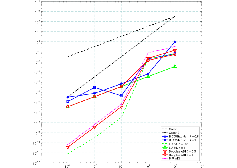
(a) Loglog order plot: $\tau$ vs. rRMSE (T=5000).

(b) Shadow removal and inpainting.

Figure 1: 0(a): Relative RMS error at $T=5000$ for several $\tau$. 0(b): Shadow removal inputs (top); Douglas ADI solution and result after non-local inpainting [1] (bottom). Parameters: $\tau=10$; $\theta=0.5$. Image from: http://aqua.cs.uiuc.edu/site/projects/shadow.html.

4 Conclusions

In this paper, we consider the image osmosis model proposed in [9, 10] for imaging applications. We proposed dimensional splitting approaches to decompose the discretised 2D operator into two tridiagonal operators. We proved that the splitting numerical schemes preserve analogous properties holding in the continuous model. Numerically, these methods are efficient and accurate. We tested the proposed methods for a shadow removal problem, with an inpainting post-processing step. Future research directions include the rigorous convergence proof of the discrete models to the continuum one as $N\to\infty$ as well as a rigorous stability and convergence analysis for the Douglas method (7).

LC acknowledges the joint ANR/FWF Project “Efficient Algorithms for Nonsmooth Optimization in Imaging” (EANOI) FWF n. I1148 / ANR-12-IS01-0003. CE acknowledges the support of GNCS-INDAM and PRIN 2012 N. 2012MTE38N. SP acknowledges UK EPSRC grant EP/L016516/1.

References

References

• [1] Arias P, Facciolo G, Caselles V and Sapiro G 2011 ICJV 93 319-347
• [2] Al-Mohy and A.H. Higham N J 2011 SIAM J. Sci. Comput. 33 488-511
• [3] Aubert G and Kornprobst P 2006 Mathematical problems in image processing: Partial Differential Equations and the Calculus of Variations 2nd ed Applied Mathematical Sciences (Springer) ISBN 9780387322001
• [4] Finlayson G, Hordley S, Lu C and Drew M 2002 ECCV in LNCS (Springer) 2353 823-836
• [5] Hundsdorfer W and Verwer J 2003 Numerical solution of time-dependent advection-diffusion-reaction equations Computational Mathematics (Springer) ISBN 9783642057076
• [6] Parisotto S, Calatroni L and Daffara C 2017, arXiv preprint: 1704.04052.
• [7] Saad Y.2003 Iterative Methods for Sparse Linear Systems 2nd ed (SIAM) ISBN 9780898715347
• [8] Schönlieb C-B 2015 Partial Differential Equation Methods for Image Inpainting Cambridge Monographs on Applied and Computational Mathematics (CUP) ISBN 9781107001008
• [9] Vogel O, Hagenburg K, Weickert and J Setzer S 2013 SSVM in LNCS (Springer) 7893 368-379
• [10] Weickert J, Hagenburg and K BreußVogel O 2013 EMMCVPR in LNCS (Springer) 8081 26-39
• [11] Weiss Y 2001 ICCV in IEEE Proceedings on ICCV 2 68-75