Multivariate Gaussian and Student$-t$ process regression for multi-output prediction

Abstract

Gaussian process model for vector-valued function has been shown to be useful for multi-output prediction. The existing method for this model is to re-formulate the matrix-variate Gaussian distribution as a multivariate normal distribution. Although it is effective in many cases, re-formulation is not always workable and is difficult to apply to other distributions because not all matrix-variate distributions can be transformed to respective multivariate distributions, such as the case for matrix-variate Student$-t$ distribution. In this paper, we propose a unified framework which is used not only to introduce a novel multivariate Student$-t$ process regression model (MV-TPR) for multi-output prediction, but also to reformulate the multivariate Gaussian process regression (MV-GPR) that overcomes some limitations of the existing methods. Both MV-GPR and MV-TPR have closed-form expressions for the marginal likelihoods and predictive distributions under this unified framework and thus can adopt the same optimization approaches as used in the conventional GPR. The usefulness of the proposed methods is illustrated through several simulated and real data examples. In particular, we verify empirically that MV-TPR has superiority for the datasets considered, including air quality prediction and bike rent prediction. At last, the proposed methods are shown to produce profitable investment strategies in the stock markets.

1 Introduction

Over the last few decades, Gaussian processes regression (GPR) has been proven to be a powerful and effective method for non-linear regression problems due to many favorable properties, such as simple structure of obtaining and expressing uncertainty in predictions, the capability of capturing a wide variety of behaviour by parameters, and a natural Bayesian interpretation [1, 2]. In 1996, Neal [3] revealed that many Bayesian regression models based on neural network converge to Gaussian processes (GP) in the limit of an infinite number of hidden units [4]. GP has been suggested as a replacement for supervised neural networks in non-linear regression [5, 6] and classification [5]. Furthermore, GP has excellent capability for forecasting time series [7, 8].

Despite the popularity of GPR in various modelling tasks, there still exists a conspicuous imperfection, that is, the majority of GPR models are implemented for single response variables or considered independently for multiple responses variables without consideration of their correlation [2, 9]. In order to resolve the multi-output prediction problem, Gaussian process regression for vector-valued function is proposed and regarded as a pragmatic and straightforward method. The core of this method is to vectorize the multi-response variables and construct a "big" covariance, which describes the correlations between the inputs as well as between the outputs [2, 9, 10, 11]. This modelling strategy is feasible due to the fact that the matrix-variate Gaussian distributions can be re-formulated as multivariate Gaussian distributions [10, 12]. Intrinsically, Gaussian process regression for vector-valued function is still a conventional Gaussian process regression model since it merely vectorizes multi-response variables, which are assumed to follow a developed case of GP with a reproduced kernel. As an extension, it is natural to consider more general elliptical processes models for multi-output prediction. However, the vectorization method cannot be used to extend multi-output GPR because the equivalence between vectorized matrix-variate and multivariate distributions only exists in Gaussian cases [12].

To overcome this drawback, in this paper we propose a unified framework which: (1) is used to introduce a novel multivariate Student$-t$ process regression model (MV-TPR) for multi-output prediction, (2) is used to reformulate the multivariate Gaussian process regression (MV-GPR) that overcomes some limitations of the existing methods, (3) can be used to derive regression models of general elliptical processes. Both MV-GPR and MV-TPR have closed-form expressions for the marginal likelihoods and predictive distributions under this unified framework and thus can adopt the same optimization approaches as used in the conventional GPR. The usefulness of the proposed methods is illustrated through several simulated examples. Furthermore, we also verify empirically that MV-TPR has superiority in the prediction based on some widely-used datasets, including air quality prediction and bike rent prediction. The proposed methods are then applied to stock market modelling which shows that the profitable stock investment strategies can be obtained.

The rest of the paper is organised as follows. Section 2 introduces some preliminaries of matrix-variate Gaussian and Student$-t$ distributions with their useful properties. Section 3 presents the unified framework to reformulate the multivariate Gaussian process regression and to derive the new multivariate Student$-t$ process regression models. Some numerical experiments by the simulated data and real data and the applications to stock market investment are presented in Section 4. Conclusion and discussion are given in Section 5.

2 Backgrounds and notations

Matrix-variate Gaussian and Student$-t$ distributions have many useful properties, as discussed in the literatures [12, 13, 14]. For completeness and easy referencing, below we list some of them which will be used in this paper.

2.1 Matrix-variate Gaussian distribution

Definition 2.1

The random matrix $X\in\mathds{R}^{n\times d}$ is said to have a matrix-variate Gaussian distribution with mean matrix $M\in\mathds{R}^{n\times d}$ and covariance matrix $\Sigma\in\mathds{R}^{n\times n},\Omega\in\mathds{R}^{d\times d}$ if and only if its probability density function is given by

$$p(X|M,\Sigma,\Omega)=(2\pi)^{-\frac{dn}{2}}\det(\Sigma)^{-\frac{d}{2}}\det(\Omega)^{-\frac{n}{2}}\mathrm{etr}(-\frac{1}{2}\Omega^{-1}(X-M)^{\mathrm{T}}\Sigma^{-1}(X-M)),$$ (1)

where $\mathrm{etr}(\cdot)$ is exponential of matrix trace, $\Omega$ and $\Sigma$ are positive semi-definite. It is denoted $X\sim\mathcal{MN}_{n,d}(M,\Sigma,\Omega)$. Without loss of clarity, it is denoted $X\sim\mathcal{MN}(M,\Sigma,\Omega)$.

Like multivariate Gaussian distribution, matrix-variate Gaussian distribution also possesses several important properties as follows.

Theorem 2.1 (Transposable)

If $X\sim\mathcal{MN}_{n,d}(M,\Sigma,\Omega)$, then $X^{\mathrm{T}}\sim\mathcal{MN}_{d,n}(M^{\mathrm{T}},\Omega,\Sigma)$.

The matrix-variate Gaussian is related to the multivariate Gaussian in the following way.

Theorem 2.2 (Vectorizable)

$X\sim\mathcal{MN}_{n,d}(M,\Sigma,\Omega)$ if and only if

$$\mathrm{vec}(X^{\mathrm{T}})\sim\mathcal{N}_{nd}(\mathrm{vec}(M^{\mathrm{T}}),\Sigma\otimes\Omega),$$

where $\mathrm{vec}(\cdot)$ is vector operator and $\otimes$ is Kronecker product (or called tensor product).

Furthermore, the matrix-variate Gaussian distribution is consistent under the marginalization and conditional distribution.

Theorem 2.3 (Marginalization and conditional distribution)

Let $X\sim\mathcal{MN}_{n,d}(M,\Sigma,\Omega)$, and partition $X,M,\Sigma$ and $\Omega$ as

$$X=\noindent\par\noindent\leavevmode\hbox{\raise-4.30554pt\hbox{\set@color\resizebox{}{}{{\leavevmode\hbox{\set@color{\ignorespaces$\displaystyle\blockarray{[c]c}X_{1r}&n_{1}\\ X_{2r}n_{2}$ }}}}}}=\noindent\par\noindent\leavevmode\hbox{\raise-4.30554pt\hbox{\set@color\resizebox{}{}{{\leavevmode\hbox{\set@color{\ignorespaces$\displaystyle\blockarray{cc}&\\ \block{[cc]}X_{1c}X_{2c}\\ d_{1}d_{2}$ }}}}}},\quad M=\noindent\par\noindent\leavevmode\hbox{\raise-4.30554pt\hbox{\set@color\resizebox{}{}{{\leavevmode\hbox{\set@color{\ignorespaces$\displaystyle\blockarray{[c]c}M_{1r}&n_{1}\\ M_{2r}n_{2}$ }}}}}}=\noindent\par\noindent\leavevmode\hbox{\raise-4.30554pt\hbox{\set@color\resizebox{}{}{{\leavevmode\hbox{\set@color{\ignorespaces$\displaystyle\blockarray{cc}&\\ \block{[cc]}M_{1c}M_{2c}\\ d_{1}d_{2}$ }}}}}}$$

$$\Sigma=\noindent\par\noindent\leavevmode\hbox{\raise-10.76385pt\hbox{\set@color\resizebox{}{}{{\leavevmode\hbox{\set@color{\ignorespaces$\displaystyle\blockarray{ccc}\block{[cc]c}\Sigma_{11}&\Sigma_{12}n_{1}\\ \Sigma_{21}\Sigma_{22}n_{2}\\ n_{1}&n_{2}$ }}}}}}\quad\text{and}\quad\Omega=\noindent\par\noindent\leavevmode\hbox{\raise-10.76385pt\hbox{\set@color\resizebox{}{}{{\leavevmode\hbox{\set@color{\ignorespaces$\displaystyle\blockarray{ccc}\block{[cc]c}\Omega_{11}&\Omega_{12}d_{1}\\ \Omega_{21}\Omega_{22}d_{2}\\ d_{1}&d_{2}$ }}}}}},$$

where $n_{1},n_{2},d_{1},d_{2}$ is the column or row length of the corresponding vector or matrix. Then,

1. $X_{1r}\sim\mathcal{MN}_{n_{1},d}\left(M_{1r},\Sigma_{11},\Omega\right)$,

   $$X_{2r}|X_{1r}\sim\mathcal{MN}_{n_{2},d}\left(M_{2r}+\Sigma_{21}\Sigma_{11}^{-1}(X_{1r}-M_{1r}),\Sigma_{22\cdot 1},\Omega\right);$$

2. $X_{1c}\sim\mathcal{MN}_{n,d_{1}}\left(M_{1c},\Sigma,\Omega_{11}\right)$,

   $$X_{2c}|X_{1c}\sim\mathcal{MN}_{n,d_{2}}\left(M_{2c}+(X_{1c}-M_{1c})\Omega_{11}^{-1}\Omega_{12},\Sigma,\Omega_{22\cdot 1}\right);$$

where $\Sigma_{22\cdot 1}$and $\Omega_{22\cdot 1}$ are the Schur complement [15] of $\Sigma_{11}$ and $\Omega_{11}$, respectively,

$$\Sigma_{22\cdot 1}=\Sigma_{22}-\Sigma_{21}\Sigma_{11}^{-1}\Sigma_{12},\quad\Omega_{22\cdot 1}=\Omega_{22}-\Omega_{21}\Omega_{11}^{-1}\Omega_{12}.$$

2.2 Matrix-variate Student$-t$ distribution

Definition 2.2

The random matrix $X\in\mathds{R}^{n\times d}$ is said to have a matrix-variate Student$-t$ distribution with the mean matrix $M\in\mathds{R}^{n\times d}$ and covariance matrix $\Sigma\in\mathds{R}^{n\times n},\Omega\in\mathds{R}^{d\times d}$ and the degree of freedom $\nu$ if and only if the probability density function is given by

$$p(X|\nu,M,\Sigma,\Omega) = \frac{\Gamma_{n}[\frac{1}{2}(\nu+d+n-1)]}{\pi^{\frac{1}{2}dn}\Gamma_{n}[\frac{1}{2}(\nu+n-1)]}\det(\Sigma)^{-\frac{d}{2}}\det(\Omega)^{-\frac{n}{2}}\times$$ (2)

$$\qquad\quad\det(\mathbf{I}_{n}+\Sigma^{-1}(X-M)\Omega^{-1}(X-M)^{\mathrm{T}})^{-\frac{1}{2}(\nu+d+n-1)},$$

where $\Omega$ and $\Sigma$ are positive semi-definite, and

$$\Gamma_{n}(\lambda)=\pi^{n(n-1)/4}\prod_{i=1}^{n}\Gamma(\lambda+\frac{1}{2}-\frac{i}{2}).$$

We denote this by $X\sim\mathcal{MT}_{n,d}(\nu,M,\Sigma,\Omega)$. Without loss of clarity, it is denoted $X\sim\mathcal{MT}(\nu,M,\Sigma,\Omega)$.

Theorem 2.4 (Expectation and covariance)

Let $X\sim\mathcal{MT}(\nu,M,\Sigma,\Omega)$, then

$$\mathbb{E}(X)=M,\quad\mathrm{cov}(\mathrm{vec}(X^{\mathrm{T}}))=\frac{1}{\nu-2}\Sigma\otimes\Omega,\nu>2.$$

Theorem 2.5 (Transposable)

If $X\sim\mathcal{MT}_{n,d}(\nu,M,\Sigma,\Omega)$, then $X^{\mathrm{T}}\sim\mathcal{MT}_{d,n}(\nu,M^{\mathrm{T}},\Omega,\Sigma).$

Theorem 2.6 (Asymptotics)

Let $X\sim\mathcal{MT}_{n,d}(\nu,M,\Sigma,\Omega)$,then $X\overset{d}{\to}\mathcal{MN}_{n,d}(M,\Sigma,\Omega)$ as $\nu\to\infty$, where "$\overset{d}{\to}$" denotes convergence in distribution.

Theorem 2.7 (Marginalization and conditional distribution)

Let $X\sim\mathcal{MT}_{n,d}(\nu,M,\Sigma,\Omega)$, and partition $X,M,\Sigma$ and $\Omega$ as

$$X=\noindent\par\noindent\leavevmode\hbox{\raise-4.30554pt\hbox{\set@color\resizebox{}{}{{\leavevmode\hbox{\set@color{\ignorespaces$\displaystyle\blockarray{[c]c}X_{1r}&n_{1}\\ X_{2r}n_{2}$ }}}}}}=\noindent\par\noindent\leavevmode\hbox{\raise-4.30554pt\hbox{\set@color\resizebox{}{}{{\leavevmode\hbox{\set@color{\ignorespaces$\displaystyle\blockarray{cc}&\\ \block{[cc]}X_{1c}X_{2c}\\ d_{1}d_{2}$ }}}}}},\quad M=\noindent\par\noindent\leavevmode\hbox{\raise-4.30554pt\hbox{\set@color\resizebox{}{}{{\leavevmode\hbox{\set@color{\ignorespaces$\displaystyle\blockarray{[c]c}M_{1r}&n_{1}\\ M_{2r}n_{2}$ }}}}}}=\noindent\par\noindent\leavevmode\hbox{\raise-4.30554pt\hbox{\set@color\resizebox{}{}{{\leavevmode\hbox{\set@color{\ignorespaces$\displaystyle\blockarray{cc}&\\ \block{[cc]}M_{1c}M_{2c}\\ d_{1}d_{2}$ }}}}}}$$

$$\Sigma=\noindent\par\noindent\leavevmode\hbox{\raise-10.76385pt\hbox{\set@color\resizebox{}{}{{\leavevmode\hbox{\set@color{\ignorespaces$\displaystyle\blockarray{ccc}\block{[cc]c}\Sigma_{11}&\Sigma_{12}n_{1}\\ \Sigma_{21}\Sigma_{22}n_{2}\\ n_{1}&n_{2}$ }}}}}}\quad\text{and}\quad\Omega=\noindent\par\noindent\leavevmode\hbox{\raise-10.76385pt\hbox{\set@color\resizebox{}{}{{\leavevmode\hbox{\set@color{\ignorespaces$\displaystyle\blockarray{ccc}\block{[cc]c}\Omega_{11}&\Omega_{12}d_{1}\\ \Omega_{21}\Omega_{22}d_{2}\\ d_{1}&d_{2}$ }}}}}},$$

where $n_{1},n_{2},d_{1},d_{2}$ is the column or row length of the corresponding vector or matrix. Then,

1. $X_{1r}\sim\mathcal{MT}_{n_{1},d}\left(\nu,M_{1r},\Sigma_{11},\Omega\right)$,

   $$X_{2r}|X_{1r}\sim \mathcal{MT}_{n_{2},d}\Big{(}\nu+n_{1},M_{2r}+\Sigma_{21}\Sigma_{11}^{-1}(X_{1r}-M_{1r}),\Sigma_{22\cdot 1},$$

   $$\Omega+(X_{1r}-M_{1r})^{\mathrm{T}}\Sigma_{11}^{-1}(X_{1r}-M_{1r})\Big{)};$$

2. $X_{1c}\sim\mathcal{MT}_{n,d_{1}}\left(,\nu,M_{1c},\Sigma,\Omega_{11}\right)$,

   $$X_{2c}|X_{1c}\sim \mathcal{MT}_{n,d_{2}}\Big{(}\nu+d_{1},M_{2c}+(X_{1c}-M_{1c})\Omega_{11}^{-1}\Omega_{12},$$

   $$\Sigma+(X_{1c}-M_{1c})\Omega_{11}^{-1}(X_{1c}-M_{1c})^{\mathrm{T}},\Omega_{22\cdot 1}\Big{)};$$

where $\Sigma_{22\cdot 1}$and $\Omega_{22\cdot 1}$ are the Schur complement of $\Sigma_{11}$ and $\Omega_{11}$, respectively,

$$\Sigma_{22\cdot 1}=\Sigma_{22}-\Sigma_{21}\Sigma_{11}^{-1}\Sigma_{12},\quad\Omega_{22\cdot 1}=\Omega_{22}-\Omega_{21}\Omega_{11}^{-1}\Omega_{12}.$$

Remark 2.1

It can be seen that matrix-variate Student$-t$ distribution has many properties similar to matrix-variate Gaussian distribution, and it converges to matrix-variate Gaussian distribution if its degree of freedom tends to infinity. However, matrix-variate Student$-t$ distribution lacks the property of vectorizability (Theorem 2.2) [12]. As a consequence Student$-t$ process regression for multiple outputs cannot be derived by vectorizing the multi-response variables. In the next section, we propose a new framework to introduce multivariate Student$-t$ process regression model.

3 Multivariate Gaussian and Student$-t$ process regression models

3.1 Multivariate Gaussian process regression (MV-GPR)

If $\bm{f}$ is a multivariate Gaussian process on $\mathcal{X}$ with vector-valued mean function $\bm{u}:\mathcal{X}\mapsto\mathds{R}^{d}$, covariance function (also called kernel) $k:\mathcal{X}\times\mathcal{X}\mapsto\mathds{R}$ and positive semi-definite parameter matrix $\Omega\in\mathds{R}^{d\times d}$, then any finite collection of vector-valued variables have a joint matrix-variate Gaussian distribution,

$$[\bm{f}(x_{1})^{\mathrm{T}},\ldots,\bm{f}(x_{n})^{\mathrm{T}}]^{\mathrm{T}}\sim\mathcal{MN}(M,\Sigma,\Omega),n\in\mathds{N},$$

where $\bm{f},\bm{u}\in\mathds{R}^{d}$ are row vectors whose components are the functions $\{f_{i}\}_{i=1}^{d}$ and $\{\mu_{i}\}_{i=1}^{d}$ respectively. Furthermore, $M\in\mathds{R}^{n\times d}$ with $M_{ij}=\mu_{j}(x_{i})$, and $\Sigma\in\mathds{R}^{n\times n}$ with $\Sigma_{ij}=k(x_{i},x_{j})$. Sometimes $\Sigma$ is called column covariance matrix while $\Omega$ is row covariance matrix. We denote $\bm{f}\sim\mathcal{MGP}(\bm{u},k,\Omega)$.

In conventional GPR methods, the noisy model $y=f(x)+\varepsilon$ is usually considered. However, for Student$-t$ process regression such a model is analytically intractable [16]. Therefore we adopt the method used in [16] and consider the noise-free regression model where the noise term is incorporated into the kernel function.

Given $n$ pairs of observations $\{(x_{i},\bm{y}_{i})\}_{i=1}^{n},x_{i}\in\mathds{R}^{p},\bm{y}_{i}\in\mathds{R}^{1\times d}$, we assume the following model

$$\bm{f} \sim \mathcal{MGP}(\bm{u},k^{\prime},\Omega),$$

$$\bm{y}_{i} = \bm{f}(x_{i}),\mbox{ for}\ i=1,\cdots,n,$$

where

$$k^{\prime}=k(x_{i},x_{j})+\delta_{ij}\sigma_{n}^{2},$$ (3)

and $\delta_{ij}=1$ if $i=j$, otherwise $\delta_{ij}=0$. Note that the second term in (3) represents the random noises.

We assume $\bm{u}=\bm{0}$ as commonly done in GPR. By the definition of multivariate Gaussian process, it yields that the collection of functions $[\bm{f}(x_{1}),\ldots,\bm{f}(x_{n})]$ follow a matrix-variate Gaussian distribution

$$[\bm{f}(x_{1})^{\mathrm{T}},\ldots,\bm{f}(x_{n})^{\mathrm{T}}]^{\mathrm{T}}\sim\mathcal{MN}(\bm{0},K^{\prime},\Omega),$$

where $K^{\prime}$ is the $n\times n$ covariance matrix of which the $(i,j)$-th element $[K^{\prime}]_{ij}=k^{\prime}(x_{i},x_{j})$.

To predict a new variable $\bm{f}_{*}=[f_{*1},\ldots,f_{*m}]^{\mathrm{T}}$ at the test locations $X_{*}=[x_{n+1},\ldots,x_{n+m}]^{\mathrm{T}}$, the joint distribution of the training observations $Y=[\bm{y}_{1}^{\mathrm{T}},\cdots,\bm{y}_{n}^{\mathrm{T}}]^{\mathrm{T}}$ and the predictive targets $\bm{f}_{*}$ are given by

$$\begin{bmatrix}Y\\ \bm{f}_{*}\end{bmatrix}\sim\mathcal{MN}\left(\bm{0},\begin{bmatrix}K^{\prime}(X,X)\quad K^{\prime}(X_{*},X)^{\mathrm{T}}\\ K^{\prime}(X_{*},X)\ \ K^{\prime}(X_{*},X_{*})\end{bmatrix},\Omega\right),$$ (4)

where $K^{\prime}(X,X)$ is an $n\times n$ matrix of which the $(i,j)$-th element $[K^{\prime}(X,X)]_{ij}=k^{\prime}(x_{i},x_{j})$, $K^{\prime}(X_{*},X)$ is an $m\times n$ matrix of which the $(i,j)$-th element $[K^{\prime}(X_{*},X)]_{ij}=k^{\prime}(x_{n+i},x_{j})$, and $K^{\prime}(X_{*},X_{*})$ is an $m\times m$ matrix with the $(i,j)$-th element $[K^{\prime}(X_{*},X_{*})]_{ij}=k^{\prime}(x_{n+i},x_{n+j})$. Thus, taking advantage of conditional distribution of multivariate Gaussian process, the predictive distribution is

$$p(\bm{f}_{*}|X,Y,X_{*})=\mathcal{MN}(\hat{M},\hat{\Sigma},\hat{\Omega}),$$ (5)

where

$$\hat{M} = K^{\prime}(X_{*},X)^{\mathrm{T}}K^{\prime}(X,X)^{-1}Y,$$ (6)

$$\hat{\Sigma} = K^{\prime}(X_{*},X_{*})-K^{\prime}(X_{*},X)^{\mathrm{T}}K^{\prime}(X,X)^{-1}K^{\prime}(X_{*},X),$$ (7)

$$\hat{\Omega} = \Omega.$$ (8)

Additionally, the expectation and the covariance are obtained,

$$\mathbb{E}[\bm{f}_{*}] = \hat{M}=K^{\prime}(X_{*},X)^{\mathrm{T}}K^{\prime}(X,X)^{-1}Y,$$ (9)

$$\mathrm{cov}(\mathrm{vec}(\bm{f}^{\mathrm{T}}_{*})) = \hat{\Sigma}\otimes\hat{\Omega}=[K^{\prime}(X_{*},X_{*})-K^{\prime}(X_{*},X)^{\mathrm{T}}K^{\prime}(X,X)^{-1}K^{\prime}(X_{*},X)]\otimes\Omega.$$ (10)

3.1.1 Kernel

Although there are two covariance matrices in the above regression model, the column covariance and the row covariance, only the column covariance depends on inputs and is considered as kernel since it contains our presumptions about the function we wish to learn and define the closeness and similarity between data points [17]. As in conventional GPR, the choice of kernels has a profound impact on the performance of multivariate Gaussian process regression (as well as multivariate Student$-t$ process regression introduced later).

A wide range of useful kernels have been proposed in the literature, such as linear, rational quadratic, and Matérn [17]. But the Squared Exponential (SE) kernel is the most commonly used due to its simple form and many desirable properties such as smoothness and integrability with other functions, although it could oversmooth the data, especially financial data.

The Squared Exponential (SE) kernel is defined as

$$k_{SE}(x,x^{\prime})=s_{f}^{2}\exp(-\frac{\|x-x^{\prime}\|^{2}}{2\ell^{2}}),$$

where $s_{f}^{2}$ is the signal variance and can also be considered as an output-scale amplitude and the parameter $\ell$ is the input (length or time) scale [18]. The kernel can also be defined by Automatic Relevance Determination (ARD)

$$k_{SEard}(\bm{x},\bm{x}^{\prime})=s_{f}^{2}\exp(-\frac{(\bm{x}-\bm{x}^{\prime})^{\mathrm{T}}\Theta^{-1}(\bm{x}-\bm{x}^{\prime})}{2}),$$

where $\Theta$ is a diagonal matrix with the element components $\{\ell_{i}^{2}\}_{i=1}^{p}$, which represents the length scales for each corresponding input dimension.

For convenience and the purpose of demonstration, SE kernel is used in all our experiments where there is only one input variable whilst SEard is used in those with multiple input variables. It should be noted that there is no technical difficulty to use other kernels in our models.

3.1.2 Parameter estimation

The hyper-parameters involved in the kernel of MV-GPR need to be estimated from the training data. Although Monte Carlo methods can perform GPR without the need of estimating hyperparameters [6, 8, 19, 20], the common approach is to estimate them by means of maximum marginal likelihood due to the high computational cost of Monte Carlo methods. $\Omega$ is an extra parameter compared to the conventional GPR model, hence the unknown parameters include the hyper-parameters in the kernel, the noise variance $\sigma_{n}^{2}$ and the row covariance parameter matrix $\Omega$.

Because $\Omega$ is positive semi-definite, it can be denoted as $\Omega=\Phi\Phi^{\mathrm{T}}$, where

$$\Phi=\left[\begin{matrix}\phi_{11}&0&\cdots&0\\ \phi_{21}&\phi_{22}&\cdots&0\\ \vdots&\vdots&\ddots&\vdots\\ \phi_{d1}&\phi_{d2}&\cdots&\phi_{dd}\\ \end{matrix}\right].$$

To guarantee the uniqueness of $\Phi$, the diagonal elements are restricted to be positive and denote $\varphi_{ii}=\ln(\phi_{ii})$ for $i=1,2,\cdots,d$.

In MV-GPR model, the observations follow a matrix-variate Gaussian distribution $Y\sim\mathcal{MN}_{n,d}(\bm{0},K^{\prime},\Omega)$ where $K^{\prime}$ is the noisy column covariance matrix with element $[K^{\prime}]_{ij}=k^{\prime}(x_{i},x_{j})$ so that $K^{\prime}=K+\sigma_{n}^{2}\mathbf{I}$ where $K$ is noise-free column covariance matrix with element $[K]_{ij}=k(x_{i},x_{j})$. As we know there are hyper-parameters in the kernel $k$ so that we can denote $K=K_{\theta}$. The hyper-parameter set denotes $\Theta=\{\theta_{1},\theta_{2},\ldots\}$, thus

$$\frac{\partial K^{\prime}}{\partial\sigma_{n}^{2}}=\mathbf{I}_{n},\quad\frac{\partial K^{\prime}}{\partial\theta_{i}}=\frac{\partial K_{\theta}}{\partial\theta_{i}}$$

According to the matrix-variate distribution, the negative log marginal likelihood of observations is

$$\mathcal{L}=\frac{nd}{2}\ln(2\pi)+\frac{d}{2}\ln\det(K^{\prime})+\frac{n}{2}\ln\det(\Omega)+\frac{1}{2}\mathrm{tr}((K^{\prime})^{-1}Y\Omega^{-1}Y^{\mathrm{T}}).$$ (11)

The derivatives of the negative log marginal likelihood with respect to parameter $\sigma_{n}^{2}$, $\theta_{i}$, $\phi_{ij}$ and $\varphi_{ii}$ are as follows

$$\frac{\partial\mathcal{L}}{\partial\sigma_{n}^{2}} =\frac{d}{2}\mathrm{tr}((K^{\prime})^{-1})-\frac{1}{2}\mathrm{tr}(\alpha_{K^{\prime}}\Omega^{-1}\alpha_{K^{\prime}}^{\mathrm{T}}),$$

$$\frac{\partial\mathcal{L}}{\partial\theta_{i}} =\frac{d}{2}\mathrm{tr}\left((K^{\prime})^{-1}\frac{\partial K_{\theta}}{\partial\theta_{i}}\right)-\frac{1}{2}\mathrm{tr}\left(\alpha_{K^{\prime}}\Omega^{-1}\alpha_{K^{\prime}}^{\mathrm{T}}\frac{\partial K_{\theta}}{\partial\theta_{i}}\right),$$

$$\frac{\partial\mathcal{L}}{\partial\phi_{ij}} =\frac{n}{2}\mathrm{tr}[\Omega^{-1}(\mathbf{E}_{ij}\Phi^{\mathrm{T}}+\Phi\mathbf{E}_{ij})]-\frac{1}{2}\mathrm{tr}[\alpha_{\Omega}(K^{\prime})^{-1}\alpha_{\Omega}^{\mathrm{T}}(\mathbf{E}_{ij}\Phi^{\mathrm{T}}+\Phi\mathbf{E}_{ij})],$$

$$\frac{\partial\mathcal{L}}{\partial\varphi_{ii}} =\frac{n}{2}\mathrm{tr}[\Omega^{-1}(\mathbf{J}_{ii}\Phi^{\mathrm{T}}+\Phi\mathbf{J}_{ii})]-\frac{1}{2}\mathrm{tr}[\alpha_{\Omega}(K^{\prime})^{-1}\alpha_{\Omega}^{\mathrm{T}}(\mathbf{J}_{ii}\Phi^{\mathrm{T}}+\Phi\mathbf{J}_{ii})],$$

where $\alpha_{K^{\prime}}=(K^{\prime})^{-1}Y$, $\alpha_{\Omega}=\Omega^{-1}Y^{\mathrm{T}}$, $\mathbf{E}_{ij}$ is the $d\times d$ elementary matrix having unity in the (i,j)-th element and zeros elsewhere, and $\mathbf{J}_{ii}$ is the same as $\mathbf{E}_{ij}$ but with the unity being replaced by $e^{\varphi_{ii}}$. The details are provided in A.2.

Hence standard gradient-based numerical optimisation techniques, such as Conjugate Gradient method, can be used to minimise the negative log marginal likelihood function to obtain the estimates of the parameters. Note that since the random noise is incorporated into the kernel function the noise variance is estimated alongside the other hyper-parameters.

3.1.3 Comparison with the existing methods

Compared with the existing multi-output GPR methods [11, 2, 9], our proposed method possesses several advantages.

Firstly, the existing methods have to vectorize the multi-output matrix in order to utilise the GPR models. It is complicated and not always workable if the numbers of outputs and observations are large. In contrast, our proposed MV-GPR has more straightforward form where the model settings, derivations and computations are all directly performed in matrix form. In particular, we use column covariance (kernel) and row covariance to capture all the correlations together in the multivariate outputs, rather than assuming a separate kernel for each output and constructing a “big” covariance matrix by Kronecker product as done in [2].

Secondly, the existing methods rely on the equivalence between vectorized matrix-variate Gaussian distribution and multivariate Gaussian distribution. However, this equivalence does not exist for other elliptical distributions such as matrix-variate Student$-t$ distribution [12]. Therefore, the existing methods for multi-output Gaussian process regression cannot be applied to Student$-t$ process regression. On the other hand, our proposed MV-GPR is based on matrix forms directly and does not require vectorization so it can naturally be extended to MV-TPR as we will do in the next subsection.

Therefore, our proposed MV-GPR provides not only a new derivation of the multi-output Gaussian process regression model, but also a unified framework to derive more general elliptical processes models.

3.2 Multivariate Student$-t$ process regression (MV-TPR)

In this subsection we propose a new nonlinear regression model for multivariate response, namely multivariate Student$-t$ process regression model (MV-TPR), using the framework discussed in the previous subsections. MV-TPR is an extension to multi-output GPR, as well as an extension to the univariate Student$-t$ process regression proposed in [16].

By definition, if $\bm{f}$ is a multivariate Student$-t$ process on $\mathcal{X}$ with parameter $\nu>2$, vector-valued mean function $\bm{u}:\mathcal{X}\mapsto\mathds{R}^{d}$, covariance function (also called kernel) $k:\mathcal{X}\times\mathcal{X}\mapsto\mathds{R}$ and positive semi-definite parameter matrix $\Omega\in\mathds{R}^{d\times d}$, then any finite collection of vector-valued variables have a joint matrix-variate Student$-t$ distribution,

$$[\bm{f}(x_{1})^{\mathrm{T}},\ldots,\bm{f}(x_{n})^{\mathrm{T}}]^{\mathrm{T}}\sim\mathcal{MT}(\nu,M,\Sigma,\Omega),n\in\mathds{N},$$

where $\bm{f},\bm{u}\in\mathds{R}^{d}$ are row vectors whose components are the functions $\{f_{i}\}_{i=1}^{d}$ and $\{\mu_{i}\}_{i=1}^{d}$ respectively. Furthermore, $M\in\mathds{R}^{n\times d}$ with $M_{ij}=\mu_{j}(x_{i})$, and $\Sigma\in\mathds{R}^{n\times n}$ with $\Sigma_{ij}=k(x_{i},x_{j})$. We denote $\bm{f}\sim\mathcal{MTP}(\nu,\bm{u},k,\Omega)$.

Therefore MV-TPR model can be formulated along the same line as MV-GPR based on the definition of multivariate Student$-t$ process. We present the model briefly below.

Given $n$ pairs of observations $\{(x_{i},\bm{y}_{i})\}_{i=1}^{n},x_{i}\in\mathds{R}^{p},\bm{y}_{i}\in\mathds{R}^{1\times d}$, we assume

$$\bm{f} \sim \mathcal{MTP}(\nu,\bm{u},k^{\prime},\Omega),\nu>2,$$

$$\bm{y}_{i} = \bm{f}(x_{i}),\mbox{ for}\ i=1,\cdots,n,$$

where $\nu$ is the degree of freedom of Student$-t$ process and the remaining parameters have the same meaning of MV-GPR model. Consequently, the predictive distribution is obtained as

$$p(\bm{f}_{*}|X,Y,X_{*})=\mathcal{MT}(\hat{\nu},\hat{M},\hat{\Sigma},\hat{\Omega}),$$ (12)

where

$$\hat{\nu} = \nu+n,$$ (13)

$$\hat{M} = K^{\prime}(X_{*},X)^{\mathrm{T}}K^{\prime}(X,X)^{-1}Y,$$ (14)

$$\hat{\Sigma} = K^{\prime}(X_{*},X_{*})-K^{\prime}(X_{*},X)^{\mathrm{T}}K^{\prime}(X,X)^{-1}K^{\prime}(X_{*},X),$$ (15)

$$\hat{\Omega} = \Omega+Y^{\mathrm{T}}K^{\prime}(X,X)^{-1}Y.$$ (16)

According to the expectation and the covariance of matrix-variate Student$-t$ distribution, the predictive mean and covariance are given by

$$\mathbb{E}[\bm{f}_{*}] =\hat{M}=K^{\prime}(X_{*},X)^{\mathrm{T}}K^{\prime}(X,X)^{-1}Y,$$ (17)

$$\mathrm{cov}(\mathrm{vec}(\bm{f}^{\mathrm{T}}_{*})) =\frac{1}{\nu+n-2}\hat{\Sigma}\otimes\hat{\Omega}$$

$$=\frac{1}{\nu+n-2}[K^{\prime}(X_{*},X_{*})-K^{\prime}(X_{*},X)^{\mathrm{T}}K^{\prime}(X,X)^{-1}K^{\prime}(X_{*},X)]$$

$$\quad\otimes(\Omega+Y^{\mathrm{T}}K^{\prime}(X,X)^{-1}Y).$$ (18)

In the MV-TPR model, the observations are followed by a matrix-variate Student$-t$ distribution $Y\sim\mathcal{MT}_{n,d}(\nu,\bm{0},K^{\prime},\Omega)$. The negative log marginal likelihood is

$$\mathcal{L} = \frac{1}{2}(\nu+d+n-1)\ln\det(\mathbf{I}_{n}+(K^{\prime})^{-1}Y\Omega^{-1}Y^{\mathrm{T}})+\frac{d}{2}\ln\det(K^{\prime})+\frac{n}{2}\ln\det(\Omega)$$

$$+\ln\Gamma_{n}\left(\frac{1}{2}(\nu+n-1)\right)-\ln\Gamma_{n}\left(\frac{1}{2}(\nu+d+n-1)\right)+\frac{1}{2}dn\ln\pi$$

$$= \frac{1}{2}(\nu+d+n-1)\ln\det(K^{\prime}+Y\Omega^{-1}Y^{\mathrm{T}})-\frac{\nu+n-1}{2}\ln\det(K^{\prime})$$

$$+\ln\Gamma_{n}\left(\frac{1}{2}(\nu+n-1)\right)-\ln\Gamma_{n}\left(\frac{1}{2}(\nu+d+n-1)\right)+\frac{n}{2}\ln\det(\Omega)+\frac{1}{2}dn\ln\pi.$$

Therefore the parameters of MV-TPR contains all the parameters in MV-GPR and one more parameter: the degree of freedom $\nu$. The derivatives of the negative log marginal likelihood with respect to parameter $\nu$,$\sigma_{n}^{2}$, $\theta_{i}$, $\phi_{ij}$ and $\varphi_{ii}$ are as follows

$$\frac{\partial\mathcal{L}}{\partial\nu} =\frac{1}{2}\ln\det(U)-\frac{1}{2}\ln\det(K^{\prime})+\frac{1}{2}\psi_{n}(\frac{1}{2}\tau)-\frac{1}{2}\psi_{n}\left(\frac{1}{2}(\tau+d)\right),$$

$$\frac{\partial\mathcal{L}}{\partial\sigma^{2}_{n}} =\frac{(\tau+d)}{2}\mathrm{tr}(U^{-1})-\frac{\tau}{2}\mathrm{tr}((K^{\prime})^{-1}),$$

$$\frac{\partial\mathcal{L}}{\partial\theta_{i}} =\frac{(\tau+d)}{2}\mathrm{tr}\left(U^{-1}\frac{\partial K_{\theta}}{\partial\theta_{i}}\right)-\frac{\tau}{2}\mathrm{tr}\left(\Sigma^{-1}\frac{\partial K_{\theta}}{\partial\theta_{i}}\right),$$

$$\frac{\partial\mathcal{L}}{\partial\phi_{ij}} =-\frac{(\tau+d)}{2}\mathrm{tr}[U^{-1}\alpha_{\Omega}^{\mathrm{T}}(\mathbf{E}_{ij}\Phi^{\mathrm{T}}+\Phi\mathbf{E}_{ij})\alpha_{\Omega}]+\frac{n}{2}\mathrm{tr}[\Omega^{-1}(\mathbf{E}_{ij}\Phi^{\mathrm{T}}+\Phi\mathbf{E}_{ij})],$$

$$\frac{\partial\mathcal{L}}{\partial\varphi_{ii}} =-\frac{(\tau+d)}{2}\mathrm{tr}[U^{-1}\alpha_{\Omega}^{\mathrm{T}}(\mathbf{J}_{ii}\Phi^{\mathrm{T}}+\Phi\mathbf{J}_{ii})\alpha_{\Omega}]+\frac{n}{2}\mathrm{tr}[\Omega^{-1}(\mathbf{J}_{ii}\Phi^{\mathrm{T}}+\Phi\mathbf{J}_{ii})],$$

where $U=K^{\prime}+Y\Omega^{-1}Y^{\mathrm{T}}$, $\tau=\nu+n-1$ and $\psi_{n}(\cdot)$ is the derivative of the function $\ln\Gamma_{n}(\cdot)$ with respect to $\nu$. The details are provided in A.3.

Remark 3.1

It is known that the marginal likelihood function in GPR models is not usually convex with respect to the hyper-parameters, therefore the optimization algorithm may converge to a local optimum whereas the global one provides better result [21]. As a result, the optimized hyper-parameters obtained by maximum likelihood estimation and the performance of GPR models may depend on the initial values of the optimization algorithm [6, 8, 22, 20]. A common strategy adopted by most GPR practitioners is a heuristic method. That is, the optimization is repeated using several initial values generated randomly from a prior distribution based on their expert opinions and experiences, for example, using 10 initial values randomly selected from a uniform distribution. The final estimates of the hyper-parameters are the ones with the largest likelihood values after convergence [6, 8, 22]. Further discussion on how to select suitable initial hyper-parameters can be found in [22, 23]. In our numerical experiments, the same heuristic method is used for both MV-GPR and MV-TPR.

4 Experiments

In this section, we demonstrate the usefulness of MV-GPR and our proposed MV-TPR using some numerical examples, including simulated data and real data.

4.1 Simulated Example

We first use simulation examples to evaluate the quality of the parameter estimation and the prediction performance of the proposed models.

4.1.1 Evaluation of parameter estimation

We generate random samples from a bivariate Gaussian process $\bm{y}\sim\mathcal{MGP}(0,k^{\prime},\Omega)$, where $k^{\prime}$ is defined as in (3) with the kernel $k_{SE}$. The hyper-parameters in $k_{SE}$ are set as $[\ell,s_{f}^{2}]=[0.5,2.5]$ and $\Omega=\left(\begin{smallmatrix}1&0.8\\ 0.8&1\end{smallmatrix}\right)$. The variance of the random noise in $k^{\prime}$ takes values $\sigma_{n}^{2}=0.1$, $0.05$ and $0.01$. As explained in Section 3.1, in our models the random noises are included in the kernel, therefore no additional random errors can be added when the random samples are generated; otherwise two random error terms will result in identifiability issues in the parameter estimation. The covariate $x$ has 100 equally spaced values in [0, 1]. We utilize the heuristic method discussed in the Remark 3.1 to estimate the parameters. The experiment is repeated 20 times and we use the parameter Median Relative Error (pMRE) as a measure of the quality of the estimates [24]:

$$\mbox{pMRE}=\mbox{median}\left\{\frac{|\hat{\theta}_{i}-\theta|}{\theta},i=1,2,\cdots 20\right\},$$

where $|\cdot|$ is the absolute value, $\hat{\theta}_{i}$ is the parameter estimates in repetition $i$ and $\theta$ is the true parameter. The results are shown in Table 1.

Table 1: The pMREs of MV-GP samples with different noise levels estimated by MV-GPR

noise level $\sigma^{2}_{n}$	0.1	0.05	0.01
$\hat{\sigma}^{2}_{n}$	0.884	0.931	0.974
$\hat{s}_{f}^{2}$	0.199	0.325	0.370
$\hat{\ell}^{2}$	0.061	0.050	0.034
$\hat{\varphi}_{11}$	1.619	1.266	0.931
$\hat{\varphi}_{22}$	1.586	1.372	0.901
$\hat{\phi}_{12}$	0.846	0.878	0.858

Table 2: The pMREs of MV-TP samples with different noise levels estimated by MV-TPR

noise level $\sigma^{2}_{n}$	0.1	0.05	0.01
$\hat{\sigma}^{2}_{n}$	0.756	0.714	0.758
$\hat{s}_{f}^{2}$	0.522	0.429	1.283
$\hat{\ell}^{2}$	0.120	0.165	0.097
$\hat{\varphi}_{11}$	1.167	1.079	0.898
$\hat{\varphi}_{22}$	1.174	1.078	0.903
$\hat{\phi}_{12}$	0.951	0.981	0.965
$\hat{\nu}$	0.192	0.247	0.245

The similar experiment is also conducted for MV-TPR, where the samples are generated from a bivariate Student$-t$ process $\bm{y}\sim\mathcal{MTP}(\nu,0,k^{\prime},\Omega)$ with the same true parameters as above and $\nu=3$. The results are reported in Table 2.

It can be seen that the length scale ${\ell}^{2}$ is well estimated in both cases, while the estimates for the parameters in the row covariance matrix (${\varphi}_{11}$, ${\varphi}_{22}$ and ${\phi}_{12}$) are not as good but reasonable. This may be because the conjugate gradient optimization algorithm does not manage to reach the global maxima of the likelihood function. Better results may be achieved using optimal design for parameter estimation as discussed in [24] In general the estimates of the parameters are closer to the true values as the noise level decreases, but the improvement in terms of estimation accuracy is not significant.

4.2 Evaluation of prediction accuracy

Now we consider a simulated data from two specific functions. The true model used to generate data is given by

$$\bm{y} = [f_{1}(x),f_{2}(x)]+[\varepsilon^{(1)},\varepsilon^{(2)}],$$

$$f_{1}(x) = 2x\cos(x),\quad f_{2}(x)=1.5x\cos(x+\pi/5),$$

where the random noise $[\varepsilon^{(1)},\varepsilon^{(2)}]\sim\mathcal{MGP}(0,k_{SE},\Omega)$. We select $k_{SE}$ with parameter $[\ell,s_{f}^{2}]=[1.001,5]$ and $\Omega=\left(\begin{smallmatrix}1&0.25\\ 0.25&1\end{smallmatrix}\right)$. The covariate $x$ has 100 equally spaced values in [-10, 10] so that a sample of 100 observations for $y_{1}$ and $y_{2}$ are obtained.

For model training, we use fewer points with one part missing so that the $z$th training data points with $z=\{3r+1\}_{r=1}^{12}\cup\{3r+2\}_{r=22}^{32}$ are selected for both $y_{1}$ and $y_{2}$. The prediction is then performed for all 100 covariate values in [-10, 10]. The RMSEs between the predicted values and the true ones from $f_{1}(x)$ and $f_{2}(x)$ are calculated. For comparison, the conventional GPR and TPR models are also applied to the two outputs independently. The above experiment is repeated 1000 times and the ARMSE (Average Root Mean Square Error), defined by

$$\text{ARMSE}=\frac{1}{1000}\sum_{i=1}^{1000}\left(\frac{1}{100}\sum_{j=1}^{100}(\hat{y}_{ij}-y_{ij})^{2}\right)^{\frac{1}{2}},$$

is calculated. Here $y_{ij}$ is the $j$th observation in the $i$th repetition and $\hat{y}_{ij}$ is the corresponding predicted value. The results are reported in Table 3 and an example of prediction is demonstrated in Figure 1.

Table 3: The ARMSE by the different models (multivariate Gaussian noisy data)

Output 1 ($y_{1}$)					Output 2 ($y_{2}$)
MV-GPR	MV-TPR	GPR	TPR		MV-GPR	MV-TPR	GPR	TPR
1.540	1.258	1.594	1.585		1.749	1.518	2.018	2.017

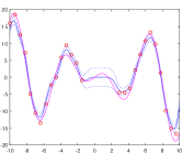
(a) MV-GPR ($y_{1}$)

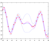
(b) MV-TPR ($y_{1}$)

(c) GPR ($y_{1}$)

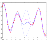
(d) TPR ($y_{1}$)

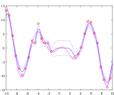
(e) MV-GPR ($y_{2}$)

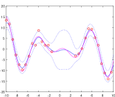
(f) MV-TPR ($y_{2}$)

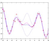
(g) GPR ($y_{2}$)

(h) TPR ($y_{2}$)

Figure 1: Predictions for MV-GP noise data using different models. From panels (a) to (d): predictions for $y_{1}$ by MV-GPR, MV-TPR, GPR and TPR. From panels (e) to (h): predictions for $y_{2}$ by MV-GPR, MV-TPR, GPR and TPR. The solid blue lines are predictions, the solid red lines are the true functions and the circles are the observations. The dash lines represent the 95% confidence intervals

The similar experiment is also conducted for the case where the random noise follows a multivariate Student$-t$ process $[\varepsilon^{(1)},\varepsilon^{(2)}]\sim\mathcal{MTP}(3,0,k_{SE},\Omega)$. We select $k_{SE}$ with parameter $[\ell,s_{f}^{2}]=[1.001,5]$ and $\Omega=\left(\begin{smallmatrix}1&0.25\\ 0.25&1\end{smallmatrix}\right)$. The resulted ARMSEs are presented in Table 4 and an example of prediction is demonstrated in Figure 2.

Table 4: The ARMSE by the different models (multivariate Student$-t$ noisy data)

Output 1 ($y_{1}$)					Output 2 ($y_{2}$)
MV-GPR	MV-TPR	GPR	TPR		MV-GPR	MV-TPR	GPR	TPR
1.441	1.238	1.505	1.503		1.636	1.464	1.941	1.940

(a) MV-GPR ($y_{1}$)

(b) MV-TPR ($y_{1}$)

(c) GPR ($y_{1}$)

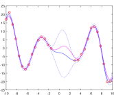
(d) TPR ($y_{1}$)

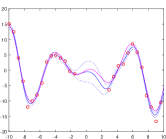
(e) MV-GPR ($y_{2}$)

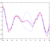
(f) MV-TPR ($y_{2}$)

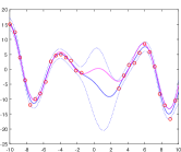
(g) GPR ($y_{2}$)

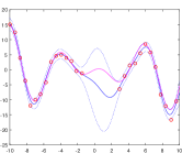
(h) TPR ($y_{2}$)

Figure 2: Predictions for MV-TP noise data using different models. From panels (a) to (d): predictions for $y_{1}$ by MV-GPR, MV-TPR, GPR and TPR. From panels (e) to (h): predictions for $y_{2}$ by MV-GPR, MV-TPR, GPR and TPR. The solid blue lines are predictions, the solid red lines are the true functions and the circles are the observations. The dash lines represent the 95% confidence intervals

From the tables and figures above, it can be seen that the multivariate process regression models are able to discover a more desired pattern in the gap compared with the conventional GPR and TPR models used independently. It also reveals that taking the correlations between the two outputs into consideration improves the accuracy of prediction compared with the methods of modelling each output independently. In particular, MV-TPR performs better than MV-GPR in the predictions for both types of noisy data whilst the performances by TPR and GPR are similar.

It is not surprising that in general MV-TPR works better than MV-GPR when the outputs have dependencies, because the former has more modelling flexibility with one more parameter which captures the degree of freedom. Theoretically, MV-TP converges to MV-GP if the degree of freedom tends to infinity, and to some extent MV-GPR is a special case of MV-TPR. In the above experiment because the observations, even generated from MV-GP, may contain outliers and the sample size (23 training points) is small, MV-TPR with a large degree of freedom may fit the data better than MV-GPR and hence provides a better prediction. These findings coincide with those in [16] in the context of univariate Student$-t$ process regressions. On the other hand, while a training sample of size 23 may be too small for two-dimensional processes such that MV-TPR performs better than MV-GPR, it may be large enough for one-dimensional processes, leading to similar performances by TPR and GPR.

It is noted that the predictive variance by MV-GPR is much smaller than the independent GPR model. This is likely due to the loss of information in the independent model.

4.3 Real data examples

We further test our proposed methods on two real datasets . The selected mean function is zero-offset and the selected kernel is SEard. Before the experiments are conducted, all the data have been normalized by

$$\tilde{y}_{i}=\frac{y_{i}-\mu}{\sigma},$$

where $\mu$ and $\sigma$ are the sample mean and standard deviation of the data $\{y_{i}\}_{i=1}^{n}$ respectively.

4.3.1 Bike rent prediction

This dataset contains the hourly and daily count of rental bikes between years 2011 and 2012 in Capital Bikeshare System with the corresponding weather and seasonal information [25]. There are 16 attributes. We test our proposed methods for multi-output prediction based on daily count dataset. After deleting all the points with missing attributes, we use the first 168 data points in the season Autumn because the data is observed on a daily basis (1 week = 7 days) and the whole dataset is divided into 8 subsets (each subset has 3 weeks’ data points). In the experiment, the input comprises 8 attributes, including normalized temperature, normalized feeling temperature, normalized humidity, normalized wind speed, whether the day is holiday or not, day of the week, working day or not and weathersit. The output consists of 2 attributes, including the count of casual users (Casual) and the count of registered users (Registered).

The cross-validation method is taken as $k-$fold, where $k=8$. Each subset is considered as a test set and the remaining subsets are considered as a training set. Four models, including MV-GPR, MV-TPR, GPR (to predict each output independently) and TPR (to predict each output independently) are applied to the data and predictions are made based on the divided training and test sets. The process is repeated for 8 times, and for each subset’s prediction, the MSE (mean square error) and the MAE (mean absolute error) is calculated. The medians of the 8 MSEs and MAEs are then used to evaluate the performance for each output. Finally, the maximum median of all the outputs (MMO) is used to evaluate the overall performance of the multi-dimensional prediction. The results are shown in Table 6(b). It can be seen that MV-TPR significantly outperforms all the other models in terms of MSE and MAE, and MV-GPR performs the second best, whilst TPR is slightly better than GPR.

Table 5: Bike rent prediction results based on MSEs and MAEs

		MV-GPR	MV-TPR	GPR	TPR
Outputs (median	Casual	0.411	0.334	0.424	0.397
of 8 subsets’ MSEs)	Registered	0.982	0.903	1.134	1.111
MMO		0.982	0.903	1.134	1.111

(a) MSE

		MV-GPR	MV-TPR	GPR	TPR
Outputs (median	Casual	0.558	0.488	0.540	0.546
of 8 subsets’ MAEs)	Registered	0.897	0.855	0.916	0.907
MMO		0.897	0.855	0.916	0.907

(b) MAE

4.3.2 Air quality prediction

The dataset contains 9,358 instances of hourly averaged responses from an array of 5 metal oxide chemical sensors embedded in an Air Quality Chemical Multisensor Device with 15 attributes [26]. We delete all the points with missing attributes (887 points remaining). The first 864 points are considered in our experiment because the data is hourly observed (1 day = 24 hours) and the whole data set is divided into 9 subsets (each subset has 4-days’ data points, totally 864 data points). In the experiment, the input comprises 9 attributes, including time, true hourly averaged concentration CO in $mg/m^{3}$ (COGT), true hourly averaged overall Non Metanic HydroCarbons concentration in $microg/m^{3}$ (NMHCGT), true hourly averaged Benzene concentration in $microg/m^{3}$ (C6H6GT), true hourly averaged NOx concentration in $ppb$ (NOx), true hourly averaged NO2 concentration in $microg/m^{3}$ (NO2), absolute humidity (AH), temperature (T) and relative humidity (RH). The output consists of 5 attributes, including PT08.S1 (tin oxide) hourly averaged sensor response, PT08.S2 (titania) hourly averaged sensor response, PT08.S3 (tungsten oxide) hourly averaged sensor response, PT08.S4 (tungsten oxide) hourly averaged sensor response and PT08.S5 (indium oxide) hourly averaged sensor response.

The cross-validation method is taken as $k-$fold, where $k=9$. The remaining modelling procedure is the same as in the bike rent prediction experiment, except that $k$ is 9 so that the process is repeated 9 times. The results are shown in Table 7(b). It can be observed that MV-TPR consistently outperforms MV-GPR, and in overall terms, MV-GPR does not perform as well as independent GPR. These results can likely be explained as follows. In fact, in our proposed framework, all the outputs are considered as a whole and the same kernel (and hyperparameters) is used for all the outputs, which may not be appropriate if different outputs have very different patterns (which is the case in this example). On the other hand, in the independent modelling different GPR models are used for different outputs and they can have different hyperparameters even though the kernel is the same, which may result in better prediction accuracy. It is noted that in this example MV-TPR still works better than MV-GPR because the former offers more modelling flexibility and is thus more robust to model misspecification. This finding is consistent with that by [16] for the univariate Student$-t$ process.

Table 6: Air quality prediction results based on MSEs and MAEs

		MV-GPR	MV-TPR	GPR	TPR
	PT08S1CO	0.091	0.065	0.079	0.074
Outputs	PT08S2NMHC	$8.16\times 10^{-5}$	$3.42\times 10^{-5}$	$1.91\times 10^{-7}$	$7.32\times 10^{-8}$
(Median of 9	PT08S3NOx	0.036	0.027	0.022	0.025
subsets’ MSEs)	PT08S4NO2	0.015	0.014	0.010	0.009
	PT08S5O3	0.092	0.073	0.060	0.067
MMO		0.092	0.073	0.079	0.074

(a) MSE

		MV-GPR	MV-TPR	GPR	TPR
	PT08S1CO	0.240	0.204	0.212	0.223
Outputs	PT08S2NMHC	$6.39\times 10^{-3}$	$1.15\times 10^{-2}$	$1.80\times 10^{-4}$	$9.26\times 10^{-5}$
(Median of 9	PT08S3NOx	0.141	0.122	0.115	0.120
subsets’ MAEs)	PT08S4NO2	0.095	0.089	0.079	0.073
	PT08S5O3	0.231	0.210	0.199	0.205
MMO		0.240	0.210	0.212	0.223

(b) MAE

4.4 Application to stock market investment

In the previous subsections, the examples show the usefulness of our proposed methods in terms of more accurate prediction. Furthermore, our proposed methods can be applied to produce trading strategies in the stock market investment.

It is known that the accurate prediction of future for an equity market is almost impossible. Admittedly, the more realistic idea is to make a strategy based on the Buy&Sell signal in the different prediction models [27]. In this paper, we consider a developed Dollar 100 (dD100) as a criterion of the prediction models. The dD100 criterion is able to reflect the theoretical future value of $100 invested at the beginning, and traded according to the signals constructed by predicted value and the reality. The details of dD100 criterion are described in Section 4.4.2.

Furthermore, the equity index is an important measurement of the value of a stock market and is used by many investors making trades and scholars studying stock markets. The index is computed from the weighted average of the selected stocks’ prices, so it is able to describe how the whole stock market in the consideration performs in a period and thus many trading strategies of a stock or a portfolio have to take the information of the index into account. As a result, our experimental predictions for specific stocks are based on the indices as well.

4.4.1 Data preparation

We obtain daily price data, containing opening, closing, and adjusted closing for the stocks (the details are shown in Section 4.4.3 and Section 4.4.4) and three main indices in the US, Dow Jones Industrial Average (INDU), S&P500 (SPX), and NASDAQ (NDX) from Yahoo Finance in the period of 2013 – 2014. The log returns of the adjusted closing price and inter-day log returns are obtained by defining

$$\text{Log return: }LR_{i}=\ln\frac{ACP_{i}}{ACP_{i-1}},$$

$$\text{Inter-day log return: }ILR_{i}=\ln\frac{CP_{i}}{OP_{i}},$$

where $ACP_{i}$ is the adjusted closing price of the $i$th day ($i>1$), $CP_{i}$ is the closing price of the $i$th day, and $OP_{i}$ is the opening price of the $i$th day. Therefore, there are totally 503 daily log returns and log inter-day returns for all the stocks and indices from 2013 to 2014.

4.4.2 Prediction model and strategy

The sliding windows method is used for our prediction models, including GPR, TPR, MV-GPR, and MV-TPR, based on the indices, INDU, SPX, and NDX. The training sample is set as 303, which is used to forecast for the next 10 days, and the training set is updated by dropping off the earliest 10 days and adding on the latest 10 days when the window is moved. The sliding-forward process was run 20 times, resulting in a total of 200 prediction days, in groups of 10. The updated training set allows all the models and parameters to adapt the dynamic structure of the equity market [27]. Specifically, the inputs consist of the log returns of 3 indices, the targets are multiple stocks’ log returns and Standard Exponential with automatic relevance determination (SEard) is used as the kernel for all of these prediction models.

It is noteworthy that the predicted log returns of stocks are used to produce a buy or sell signal for trading rather than to discover an exact pattern of the future. The signal $BS$ produced by the predicted log returns of the stocks is defined by

$$BS_{i}=\hat{LR}_{i}-LR_{i}+ILR_{i},i=1,\cdots,200,$$

where $\{\hat{LR}_{i}\}_{i=1}^{200}$ are the predicted log returns of a specific stock, $\{LR_{i}\}_{i=1}^{200}$ are the true log returns while $\{ILR_{i}\}_{i=1}^{200}$ are the inter-day log returns. The Buy&Sell strategy relying on the signal $BS$ is described in Table 7.

Table 7: Buy&Sell strategy of dD100 investment

Decision	Condition
Buy	$\hat{LR}_{i}>0$, & $BS_{i}>0$ & we have the position of cash
Sell	$\hat{LR}_{i}<0$, & $BS_{i}<0$ & we have the position of share
Keep	No action is taken for the rest of the option

It is noted that the stocks in our experiment are counted in Dollar rather than the number of shares, which means in theory we can precisely buy or sell a specific Dollar valued stock. For example, if the stock price is $37 when we only have $20, we can still buy $20 valued stock rather than borrowing $17 and then buy 1 share. Furthermore, it is also necessary to explain why we choose the signal $BS$. By the definition, we rewrite it as

$$BS_{i} = \ln(\frac{\hat{ACP}_{i}}{ACP_{i-1}})-\ln(\frac{ACP_{i}}{ACP_{i-1}})+\ln(\frac{CP_{i}}{OP_{i}})$$

$$= \ln(\frac{\hat{ACP}_{i}}{ACP_{i-1}})-\ln(\frac{ACP_{i}}{ACP_{i-1}})+\ln(\frac{ACP_{i}}{AOP_{i}})$$

$$= \ln(\frac{\hat{ACP}_{i}}{AOP_{i}}),$$

where $\{ACP_{i}\}_{i=0}^{200}$ are the last 201 adjusted closing prices for a stock, $\{CP\}_{i=1}^{200}$ are the last 200 closing prices, and $\{AOP\}_{i=1}^{200}$ are the adjusted opening prices. If $BS_{i}>0$, the predicted closing price should be higher than the adjusted opening price, which means we can obtain the inter-day profit by buying the shares at the opening price as long as the signal based on our predictions is accurate. Meanwhile, the opposite manipulation based on BS strategy means that we can avoid the inter-day loss by selling decisively at the opening price. Furthermore, the reasonable transaction fee 0.025% is considered in the experiment since the strategy might trade frequently . As a result, this is a reasonable strategy since we can definitely obtain a profit by buying the shares and cut the loss by selling the shares in time only if our prediction has no serious problem. It is also an executable strategy because the decision is made based on the next day’s reality and our prediction models.

At last, $BS$ signal varies in different prediction models so that we denote these Buy&Sell strategies based on MV-GPR, MV-TPR, GPR, and TPR model as MV-GPR strategy, MV-TPR strategy, GPR strategy, and TPR strategy, respectively.

4.4.3 Chinese companies in NASDAQ

In recent years, the "Chinese concepts stock" has received an extensive attention among international investors owing to the fast development of Chinese economy and an increasing number of Chinese firms have been traded in the international stock markets [28]. The "Chinese concepts stock" refers to the stock issued by firms whose asset or earning have essential activities in Mainland China. Undoubtedly, all these "Chinese concept stocks" are heavily influenced by the political and economic environment of China together. For this reason, all these stocks have the potential and unneglectable correlation theoretically, which is probably reflected in the movement of stock prices. The performance of multiple targets prediction, which takes the potential relationship into consideration, should be better. Therefore, the first real data example is based on 3 biggest Chinese companies described in Table 8.

Table 8: Three biggest "Chinese concept" stocks

Ticker	Exchange	Company
BIDU	NASDAQ	Baidu, Inc.
CTRP	NASDAQ	Ctrip.com International, Ltd.
NTES	NASDAQ	NetEase, Inc.

We apply MV-GPR, MV-TPR, GPR and TPR strategies and the results are demonstrated in Figure 3. Furthermore, Table B1, Table B2 and Table B3 in the appendix summarize the results by period for each stock respectively. In particular, the Buy&Sell signal examples for each stock are shown in Table B4, Table B5 and Table B6 respectively, along with other relevant details.

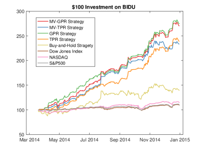
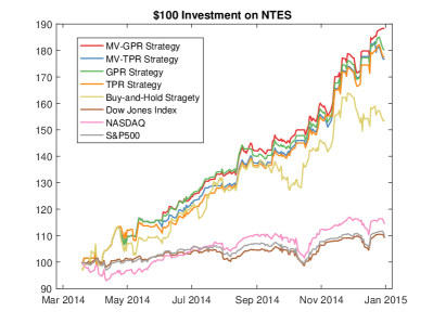
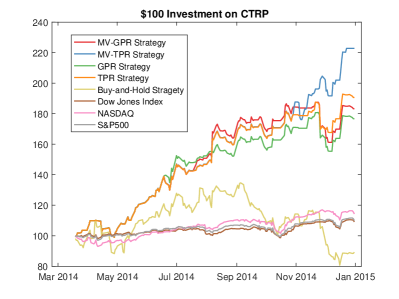
Figure 3: The movement of invested $100 in 200 days for 3 Chinese stocks in the US market. The top 4 lines in legend are Buy&Sell strategies based on 4 prediction models, MV-GPR, MV-TPR, GPR, and TPR, respectively. The last 4 lines are Buy&Hold strategies for the stock and for the three indices, INDU, NASDAQ, and NDX, respectively

From the view of Figure 3, there is no doubt that a $100 investment for each stock has sharply increased over 200 days period using Buy&Sell strategies no matter whether the stock went up or down during this period. In particular, the stock prices of BIDU and NTES rose up gradually while CTRP hit the peak and then decreased in a large scale. Anyway, the Buy&Sell strategies based on different prediction models have still achieved considerable profits compared with Buy&Hold strategies for the corresponding investments. However, the different prediction models have diverse performances for each stock. For BIDU, GPR-based models, including MV-GPR and GPR, outperform TPR-based models, including MV-TPR and TPR. For NTES, all the models for Buy&Sell strategy have a similar performance. Admittedly, TPR-based models, especially MV-TPR, have an outstanding performance for stock CTRP.

4.4.4 Diverse sectors in Dow 30

Owing to the globalization of capital, there has been a significant shift in the relative importance of national and economic influences in the world’s largest equity markets and the impact of industrial sector effects is now gradually replacing that of country effects in these markets [29]. Therefore, a further example is carried out under the diverse industrial sectors in Dow 30 from New York Stock Exchange (NYSE) and NASDAQ.

Initially, the classification of stocks based on diverse industrial sectors in Dow 30 has to be done. There are two main industry classification taxonomies, including Industry Classification Benchmark (ICB) and Global Industry Classification Standard (GICS). In our research, ICB is used to segregate markets into sectors within the macroeconomy. The stocks in Dow 30 are classified in Table 9.

Table 9: Stock components of Dow 30

Ticker	Company	Exchange	Industry	Industry (ICB)
DD	DuPont	NYSE	Chemical industry	Basic Materials
KO	Coca-Cola	NYSE	Beverages	Consumer Goods
PG	Procter & Gamble	NYSE	Consumer goods	Consumer Goods
MCD	McDonald’s	NYSE	Fast food	Consumer Goods
NKE	Nike	NYSE	Apparel	Consumer Services
DIS	Walt Disney	NYSE	Broadcasting and entertainment	Consumer Services
HD	The Home Depot	NYSE	Home improvement retailer	Consumer Services
WMT	Wal-Mart	NYSE	Retail	Consumer Services
JPM	JPMorgan Chase	NYSE	Banking	Financials
GS	Goldman Sachs	NYSE	Banking, Financial services	Financials
V	Visa	NYSE	Consumer banking	Financials
AXP	American Express	NYSE	Consumer finance	Financials
TRV	Travelers	NYSE	Insurance	Financials
UNH	UnitedHealth Group	NYSE	Managed health care	Health Care
JNJ	Johnson & Johnson	NYSE	Pharmaceuticals	Health Care
MRK	Merck	NYSE	Pharmaceuticals	Health Care
PFE	Pfizer	NYSE	Pharmaceuticals	Health Care
BA	Boeing	NYSE	Aerospace and defense	Industrials
MMM	3M	NYSE	Conglomerate	Industrials
GE	General Electric	NYSE	Conglomerate	Industrials
UTX	United Technologies	NYSE	Conglomerate	Industrials
CAT	Caterpillar	NYSE	Construction and mining equipment	Industrials
CVX	Chevron	NYSE	Oil & gas	Oil & Gas
XOM	ExxonMobil	NYSE	Oil & gas	Oil & Gas
CSCO	Cisco Systems	NASDAQ	Computer networking	Technology
IBM	IBM	NYSE	Computers and technology	Technology
AAPL	Apple	NASDAQ	Consumer electronics	Technology
INTC	Intel	NASDAQ	Semiconductors	Technology
MSFT	Microsoft	NASDAQ	Software	Technology
VZ	Verizon	NYSE	Telecommunication	Telecommunications

Due to the multivariate process models considering at least two related stocks in one group, the first (Basic Materials) and the last industrial sector (Telecommunications), each consisting of only one stock, are excluded. As a result, our experiments are performed seven times for the seven grouped industrial sector stocks, including Oil&Gas, Industrial, Consumer Goods, Health Care, Consumer Services, Financials and Technology, respectively.

Secondly, the 4 models, MV-GPR, MV-TPR, GPR and TPR, are applied in the same way as in Section 4.4.3 and the ranking of stock investment performance is listed in Table 10 (the details are summarized in Table C1). On the whole, for each stock, there is no doubt that using Buy&Sell strategy is much better than using Buy&Hold strategy regardless of the industrial sector. Specifically, MV-GPR makes a satisfactory performance overall in the sectors, Industrials, Consumer Services and Financials while MV-TPR has a higher ranking in Health Care in general.

Table 10: Stock investment performance ranking under different strategies

Ticker	Industry	Buy&Sell Strategy				Buy&Hold Stragegy
		MV-GPR	MV-TPR	GPR	TPR	Stock	INDU	NDX	SPX
CVX	Oil & Gas	3rd	4th	2nd	1st	8th	7th	5th	6th
XOM	Oil & Gas	4th	2nd	3rd	1st	8th	7th	5th	6th
MMM	Industrials	2nd	3rd	1st	4th	5th	8th	6th	7th
BA	Industrials	1st	2nd	3rd	4th	8th	7th	5th	6th
CAT	Industrials	3rd	4th	2nd	1st	8th	7th	5th	6th
GE	Industrials	2nd	4th	3rd	1st	8th	7th	5th	6th
UTX	Industrials	2nd	4th	3rd	1st	8th	7th	5th	6th
KO	Consumer Goods	2nd	1st	3rd	4th	6th	8th	5th	7th
MCD	Consumer Goods	2nd	4th	1st	3rd	8th	7th	5th	6th
PG	Consumer Goods	3rd	4th	1st	2nd	5th	8th	6th	7th
JNJ	Health Care	3rd	2nd	1st	4th	6th	8th	5th	7th
MRK	Health Care	3rd	2nd	4th	1st	8th	7th	5th	6th
PFE	Health Care	4th	1st	3rd	2nd	8th	7th	5th	6th
UNH	Health Care	2nd	3rd	1st	4th	5th	8th	6th	7th
HD	Consumer Services	1st	4th	3rd	2nd	5th	8th	6th	7th
NKE	Consumer Services	2nd	3rd	4th	1st	5th	8th	6th	7th
WMT	Consumer Services	1st	4th	3rd	2nd	5th	8th	6th	7th
DIS	Consumer Services	3rd	2nd	1st	4th	5th	8th	6th	7th
AXP	Financials	2nd	4th	1st	3rd	8th	7th	5th	6th
GS	Financials	2nd	1st	3rd	4th	5th	8th	6th	7th
JPM	Financials	2nd	4th	1st	3rd	6th	8th	5th	7th
TRV	Financials	2nd	3rd	1st	4th	5th	8th	6th	7th
V	Financials	1st	4th	3rd	2nd	5th	8th	6th	7th
AAPL	Technology	4th	2nd	3rd	1st	5th	8th	6th	7th
CSCO	Technology	2nd	1st	3rd	4th	5th	8th	6th	7th
IBM	Technology	4th	1st	2nd	3rd	8th	7th	5th	6th
INTC	Technology	3rd	4th	2nd	1st	5th	8th	6th	7th
MSFT	Technology	2nd	4th	1st	3rd	5th	8th	6th	7th

Further analysis is considered using industrial sector portfolios, which consists of these grouped stocks by the same weight investment on each stock. For example, the Oil & Gas portfolio investment is $100 with $50 shares CVX and $50 shares XOM while the Technology portfolio investment is $100 with the same $20 investment on each stock in the industrial sector Technology. The diverse industry portfolio investment performance ranking is listed in Table 11 (the details are described in Table C2). Apparently, the Buy&Sell strategies performed better than the Buy&Hold strategies. MV-GPR suits better in three industries, including Consumer Goods, Consumer Services, and Financials, followed by TPR which performed best in Oil&Gas and Industrials. The optimal investment strategy in Health Care is MV-TPR while in Technology industry, using GPR seems to be the most profitable.

Table 11: Industry portfolio investment performance ranking under different strategies

Industry Portfolio	Buy&Sell Strategy				Buy&Hold Stragegy
	MV-GPR	MV-TPR	GPR	TPR	Stock	INDU	NDX	SPX
Oil & Gas	4th	3rd	2nd	1st	8th	7th	5th	6th
Industrials	2nd	4th	3rd	1st	8th	7th	5th	6th
Consumer Goods	1st	4th	2nd	3rd	7th	8th	5th	6th
Health Care	4th	1st	3rd	2nd	6th	8th	5th	7th
Consumer Services	1st	4th	3rd	2nd	5th	8th	6th	7th
Financials	1st	4th	2nd	3rd	5th	8th	6th	7th
Technology	4th	3rd	1st	2nd	5th	8th	6th	7th

5 Conclusion and discussion

In this paper we have proposed a unified framework for multi-output regression and prediction. Using this framework, we introduced a novel multivariate Student$-t$ process regression model (MV-TPR) and also reformulated the multivariate Gaussian process regression (MV-GPR) which overcomes some limitations of the existing methods. It could also be used to derive regression models of general elliptical processes. Under this framework, the model settings, derivations and computations for both MV-GPR and MV-TPR are all directly performed in matrix form. MV-GPR is a more straightforward method compared to the existing vectorization method and can be implemented in the same way as the conventional GPR. Similar to the existing Gaussian process regression for vector-valued function, our models are also able to learn the correlations between inputs and outputs, but with more convenient and flexible formulations. The proposed MV-TPR also possesses closed-form expressions for the marginal likelihood and the predictive distributions under this unified framework. Thus the same optimization approaches as used in the conventional GPR can be adopted. The usefulness of the proposed methods is illustrated through several numerical examples. It is empirically demonstrated that MV-TPR has superiority in prediction in these examples, including the simulated examples, air quality prediction and bike rent prediction.

The proposed methods are also applied to stock market modelling and are shown to have the ability to make a profitable stock investment. For the three "Chinese concept stocks", the Buy&Sell strategies based on the proposed models have more satisfactory performances, compared with the Buy&Hold strategies for the corresponding stocks and three main indices in the US; in particular, the strategy based on MV-TPR has outstanding returns for NetEase among three stocks. When applied to the industrial sectors in Dow 30, the results indicate that the strategies based on MV-GPR have generally considerable performances in Industrials, Consumer Goods, Consumer Services, and Financials sectors, while those based on MV-TPR can make maximum profit in Health Care sector.

It is noted that we used the squared exponential kernel for demonstration in all our experiments. However, it can be expected that other kernels or more complicated kernels may lead to better results, especially in the financial data examples, as the SE kernel may oversmooth data; see [17] for more details on the choice of kernels. In this paper we assume that different outputs are observed at the same covariate values. In practice, different responses may be observed at different locations. These cases are, however, difficult for the proposed framework since all the outputs have to be considered as a matrix in our models, rather than as a vector with adjustable length. Another issue worth noting is that, as discussed in Section 4.3.2, in our proposed framework all the outputs are considered as a whole and the same kernel (and hyperparameters) is used for all the outputs, which may not be appropriate if different outputs have very different patterns such as in the air quality example. Moreover, it is also important to further study how to improve the quality of the parameter estimates, for example using optimal design methods for parameter estimation as discussed in [24]. All of these problems are worth further investigation and exploration and will be our future works.

Appendix A Negative Log Marginal Likelihood and Gradient Evaluation

A.1 Matrix derivatives

According to the chain rule of derivatives of matrix, there exists [30]: Letting $U=f(X)$, the derivatives of the function $g(U)$ with respect to X are

$$\frac{\partial g(U)}{\partial X_{ij}}=\mathrm{tr}\left[\left(\frac{\partial g(U)}{\partial U}\right)^{\mathrm{T}}\frac{\partial U}{\partial X_{ij}}\right],$$

where X is an $n\times m$ matrix. Additionally, there are another two useful formulas of derivative with respect to X.

$$\frac{\partial\ln\det(X)}{\partial X}=X^{-\mathrm{T}},\quad\frac{\partial}{\partial X}\mathrm{tr}(AX^{-1}B)=-(X^{-1}BAX^{-1})^{\mathrm{T}},$$

where X is an $n\times n$ matrix, A is a constant $m\times n$ matrix and B is a constant $n\times m$ matrix.

A.2 Multivariate Gaussian process regression

For a matrix-variate observations $Y\sim\mathcal{MN}_{n,d}(M,\Sigma,\Omega)$ where $M\in\mathds{R}^{n\times d},\Sigma\in\mathds{R}^{n\times n},\Omega\in\mathds{R}^{d\times d}$, the negative log likelihood is

$$\mathcal{L}=\frac{nd}{2}\ln(2\pi)+\frac{d}{2}\ln\det(\Sigma)+\frac{n}{2}\ln\det(\Omega)+\frac{1}{2}\mathrm{tr}(\Sigma^{-1}(Y-M)\Omega^{-1}(Y-M)^{\mathrm{T}}),$$ (19)

where actually $\Sigma=K+\sigma_{n}^{2}\mathbf{I}$ As we know there are several parameters in the kernel $k$ so that we can denote $K=K_{\theta}$. The parameter set denotes $\Theta=\{\theta_{1},\theta_{2},\ldots\}$. Besides, we denote the parameter matrix $\Omega=\Phi\Phi^{\mathrm{T}}$ since $\Omega$ is positive semi-definite, where

$$\Phi=\left[\begin{matrix}\phi_{11}&0&\cdots&0\\ \phi_{21}&\phi_{22}&\cdots&0\\ \vdots&\vdots&\ddots&\vdots\\ \phi_{d1}&\phi_{d2}&\cdots&\phi_{dd}\\ \end{matrix}\right].$$

To guarantee the uniqueness of $\Phi$, the diagonal elements are restricted to be positive and denote $\varphi_{ii}=\ln(\phi_{ii})$ for $i=1,2,\cdots,d$. Therefore,

$$\frac{\partial\Sigma}{\partial\sigma_{n}^{2}}=\mathbf{I}_{n},\quad\frac{\partial\Sigma}{\partial\theta_{i}}=\frac{\partial K^{\prime}_{\theta}}{\partial\theta_{i}},\qquad\frac{\partial\Omega}{\partial\phi_{ij}}=\mathbf{E}_{ij}\Phi^{\mathrm{T}}+\Phi\mathbf{E}_{ij},\quad\frac{\partial\Omega}{\partial\varphi_{ii}}=\mathbf{J}_{ii}\Phi^{\mathrm{T}}+\Phi\mathbf{J}_{ii},$$

where $\mathbf{E}_{ij}$ is the $d\times d$ elementary matrix having unity in the (i,j)-th element and zeros elsewhere, and $\mathbf{J}_{ii}$ is the same as $\mathbf{E}_{ij}$ but with the unity being replaced by $e^{\varphi_{ii}}$.

The derivatives of the negative log likelihood with respect to $\sigma_{n}^{2}$, $\theta_{i}$, $\phi_{ij}$ and $\varphi_{ii}$ are as follows. The derivative with respect to $\theta_{i}$ is

$$\frac{\partial\mathcal{L}}{\partial\theta_{i}} = \frac{d}{2}\frac{\partial\ln\det(\Sigma)}{\partial\theta_{i}}+\frac{1}{2}\frac{\partial}{\partial\theta_{i}}\mathrm{tr}(\Sigma^{-1}(Y-M)\Omega^{-1}(Y-M)^{\mathrm{T}})$$ (20)

$$= \frac{d}{2}\mathrm{tr}\left[\left(\frac{\partial\ln\det(\Sigma)}{\partial\Sigma}\right)^{\mathrm{T}}\frac{\partial\Sigma}{\partial\theta_{i}}\right]+\frac{1}{2}\mathrm{tr}\left[\left(\frac{\partial\mathrm{tr}(\Sigma^{-1}G)}{\partial\Sigma}\right)^{\mathrm{T}}\frac{\partial\Sigma}{\partial\theta_{i}}\right]$$

$$= \frac{d}{2}\mathrm{tr}\left(\Sigma^{-1}\frac{\partial K^{\prime}_{\theta}}{\partial\theta_{i}}\right)-\frac{1}{2}\mathrm{tr}\left(\Sigma^{-1}G\Sigma^{-1}\frac{\partial K^{\prime}_{\theta}}{\partial\theta_{i}}\right)$$

$$= \frac{d}{2}\mathrm{tr}\left(\Sigma^{-1}\frac{\partial K^{\prime}_{\theta}}{\partial\theta_{i}}\right)-\frac{1}{2}\mathrm{tr}\left(\alpha_{\Sigma}\Omega^{-1}\alpha_{\Sigma}^{\mathrm{T}}\frac{\partial K^{\prime}_{\theta}}{\partial\theta_{i}}\right),$$

where $G=(Y-M)\Omega^{-1}(Y-M)^{\mathrm{T}}$ and $\alpha_{\Sigma}=\Sigma^{-1}(Y-M)$.The fourth equality is due to the symmetry of $\Sigma$.

Due to $\partial\Sigma/\partial\sigma^{2}_{n}=\mathbf{I}_{n}$, the derivative with respect to $\sigma_{n}^{2}$ is:

$$\frac{\partial\mathcal{L}}{\partial\sigma_{n}^{2}} = \frac{d}{2}\mathrm{tr}(\Sigma^{-1})-\frac{1}{2}\mathrm{tr}(\alpha_{\Sigma}\Omega^{-1}\alpha_{\Sigma}^{\mathrm{T}}).$$ (21)

Letting $\alpha_{\Omega}=\Omega^{-1}(Y-M)^{\mathrm{T}}$, the derivative with respect to $\phi_{ij}$ is

$$\frac{\partial\mathcal{L}}{\partial\phi_{ij}} = \frac{n}{2}\frac{\partial\ln\det(\Omega)}{\partial\phi_{ij}}+\frac{1}{2}\frac{\partial}{\partial\phi_{ij}}\mathrm{tr}(\Sigma^{-1}(Y-M)\Omega^{-1}(Y-M)^{\mathrm{T}})$$ (22)

$$= \frac{n}{2}\mathrm{tr}\left(\Omega^{-1}\frac{\partial\Omega}{\partial\phi_{ij}}\right)-\frac{1}{2}\mathrm{tr}\left[((\Omega^{-1}(Y-M)^{\mathrm{T}}\Sigma^{-1}(Y-M)\Omega^{-1})^{\mathrm{T}})^{\mathrm{T}}\frac{\partial\Omega}{\partial\phi_{ij}}\right]$$

$$= \frac{n}{2}\mathrm{tr}\left(\Omega^{-1}\frac{\partial\Omega}{\partial\phi_{ij}}\right)-\frac{1}{2}\mathrm{tr}\left(\alpha_{\Omega}\Sigma^{-1}\alpha_{\Omega}^{\mathrm{T}}\frac{\partial\Omega}{\partial\phi_{ij}}\right)$$

$$= \frac{n}{2}\mathrm{tr}[\Omega^{-1}(\mathbf{E}_{ij}\Phi^{\mathrm{T}}+\Phi\mathbf{E}_{ij})]-\frac{1}{2}\mathrm{tr}[\alpha_{\Omega}\Sigma^{-1}\alpha_{\Omega}^{\mathrm{T}}(\mathbf{E}_{ij}\Phi^{\mathrm{T}}+\Phi\mathbf{E}_{ij})],$$

where the third equation is due to the symmetry of $\Omega$. Similarly, the derivative with respect to $\varphi_{ii}$ is

$$\frac{\partial\mathcal{L}}{\partial\varphi_{ii}} = \frac{n}{2}\frac{\partial\ln\det(\Omega)}{\partial\varphi_{ii}}+\frac{1}{2}\frac{\partial}{\partial\varphi_{ii}}\mathrm{tr}(\Sigma^{-1}(Y-M)\Omega^{-1}(Y-M)^{\mathrm{T}})$$ (23)

$$= \frac{n}{2}\mathrm{tr}[\Omega^{-1}(\mathbf{J}_{ii}\Phi^{\mathrm{T}}+\Phi\mathbf{J}_{ii})]-\frac{1}{2}\mathrm{tr}[\alpha_{\Omega}\Sigma^{-1}\alpha_{\Omega}^{\mathrm{T}}(\mathbf{J}_{ii}\Phi^{\mathrm{T}}+\Phi\mathbf{J}_{ii})].$$

A.3 Multivariate Student$-t$ process regression

The negative log likelihood of observations $Y\sim\mathcal{MT}_{n,d}(\nu,M,\Sigma,\Omega)$ where $M\in\mathds{R}^{n\times d},\Sigma\in\mathds{R}^{n\times n},\Omega\in\mathds{R}^{d\times d}$, is

$$\mathcal{L} = \frac{1}{2}(\nu+d+n-1)\ln\det(\mathbf{I}_{n}+\Sigma^{-1}(Y-M)\Omega^{-1}(Y-M)^{\mathrm{T}})$$

$$+\frac{d}{2}\ln\det(\Sigma)+\frac{n}{2}\ln\det(\Omega)+\ln\Gamma_{n}\left(\frac{1}{2}(\nu+n-1)\right)+\frac{1}{2}dn\ln\pi$$

$$-\ln\Gamma_{n}\left(\frac{1}{2}(\nu+d+n-1)\right)$$

$$= \frac{1}{2}(\nu+d+n-1)\ln\det(\Sigma+(Y-M)\Omega^{-1}(Y-M)^{\mathrm{T}})-\frac{\nu+n-1}{2}\ln\det(\Sigma)$$

$$+\ln\Gamma_{n}\left(\frac{1}{2}(\nu+n-1)\right)-\ln\Gamma_{n}\left(\frac{1}{2}(\nu+d+n-1)\right)$$

$$+\frac{n}{2}\ln\det(\Omega)+\frac{1}{2}dn\ln\pi.$$

Letting $U=\Sigma+(Y-M)\Omega^{-1}(Y-M)^{\mathrm{T}}$ and $\alpha_{\Omega}=\Omega^{-1}(Y-M)^{\mathrm{T}}$, the derivative of U with respect to $\sigma_{n}^{2}$, $\theta_{i}$,$\nu$, $\phi_{ij}$ and $\varphi_{ii}$ are

$$\frac{\partial U}{\partial\sigma_{n}^{2}}=\mathbf{I}_{n},\quad\frac{\partial U}{\partial\theta_{i}}=\frac{\partial K^{\prime}_{\theta}}{\partial\theta_{i}},\quad\frac{\partial U}{\partial\nu}=\mathrm{0},$$ (24)

$$\frac{\partial U}{\partial\phi_{ij}} = -(Y-M)\Omega^{-1}\frac{\partial\Omega}{\partial\phi_{ij}}\Omega^{-1}(Y-M)^{\mathrm{T}}=-\alpha_{\Omega}^{\mathrm{T}}\frac{\partial\Omega}{\partial\phi_{ij}}\alpha_{\Omega},$$ (25)

$$\frac{\partial U}{\partial\varphi_{ii}} = -(Y-M)\Omega^{-1}\frac{\partial\Omega}{\partial\varphi_{ii}}\Omega^{-1}(Y-M)^{\mathrm{T}}=-\alpha_{\Omega}^{\mathrm{T}}\frac{\partial\Omega}{\partial\varphi_{ii}}\alpha_{\Omega}.$$ (26)

Therefore, the derivative of negative log marginal likelihood with respect to $\theta_{i}$ is

$$\frac{\partial\mathcal{L}}{\partial\theta_{i}} = \frac{(\tau+d)}{2}\frac{\partial\ln\det(U)}{\partial\theta_{i}}-\frac{\tau}{2}\frac{\partial\ln\det(\Sigma)}{\partial\theta_{i}}$$ (27)

$$= \frac{(\tau+d)}{2}\mathrm{tr}\left(U^{-1}\frac{\partial K^{\prime}_{\theta}}{\partial\theta_{i}}\right)-\frac{\tau}{2}\mathrm{tr}\left(\Sigma^{-1}\frac{\partial K^{\prime}_{\theta}}{\partial\theta_{i}}\right),$$

where the constant $\tau=\nu+n-1$.

The derivative with respect to $\sigma_{n}^{2}$ is

$$\frac{\partial\mathcal{L}}{\partial\sigma^{2}_{n}}=\frac{(\tau+d)}{2}\mathrm{tr}(U^{-1})-\frac{\tau}{2}\mathrm{tr}(\Sigma^{-1}).$$ (28)

The derivative with respect to $\nu$ is

$$\frac{\partial\mathcal{L}}{\partial\nu}=\frac{1}{2}\ln\det(U)-\frac{1}{2}\ln\det(\Sigma)+\frac{1}{2}\psi_{n}(\frac{1}{2}\tau)-\frac{1}{2}\psi_{n}[\frac{1}{2}(\tau+d)]$$ (29)

where $\psi_{n}(\cdot)$ is the derivative of the function $\ln\Gamma_{n}(\cdot)$ with respect to $\nu$.

The derivative of $\mathcal{L}$ with respect to $\phi_{ij}$ is

$$\frac{\partial\mathcal{L}}{\partial\phi_{ij}} = \frac{(\tau+d)}{2}\frac{\partial\ln\det(U)}{\partial\phi_{ij}}+\frac{n}{2}\frac{\partial\ln\det(\Omega)}{\partial\phi_{ij}}$$ (30)

$$= -\frac{(\tau+d)}{2}\mathrm{tr}[U^{-1}\alpha_{\Omega}^{\mathrm{T}}(\mathbf{E}_{ij}\Phi^{\mathrm{T}}+\Phi\mathbf{E}_{ij})\alpha_{\Omega}]+\frac{n}{2}\mathrm{tr}[\Omega^{-1}(\mathbf{E}_{ij}\Phi^{\mathrm{T}}+\Phi\mathbf{E}_{ij})].$$

Similarly, the derivative with respect to $\varphi_{ii}$ is

$$\frac{\partial\mathcal{L}}{\partial\varphi_{ii}}=-\frac{(\tau+d)}{2}\mathrm{tr}[U^{-1}\alpha_{\Omega}^{\mathrm{T}}(\mathbf{J}_{ii}\Phi^{\mathrm{T}}+\Phi\mathbf{J}_{ii})\alpha_{\Omega}]+\frac{n}{2}\mathrm{tr}[\Omega^{-1}(\mathbf{J}_{ii}\Phi^{\mathrm{T}}+\Phi\mathbf{J}_{ii})].$$ (31)

Appendix B Three Chinese Stocks Investment Details

Table B1: The movement of invested $100 for 200 days split in to 20 periods (Stock: BIDU)

Forecast terms	Buy&Sell decisions by prediction models				Buy&Hold stock/index
	MV-GPR	MV-TPR	GPR	TPR	BIDU	INDU	NDX	SPX
Beginning ($)	100				100
Period 1	103.53	100.97	103.53	100.97	97.14	101.20	98.70	100.71
Period 2	109.80	106.09	115.60	102.03	94.87	99.55	94.10	98.44
Period 3	108.37	104.71	115.96	100.71	93.89	101.50	96.64	100.62
Period 4	117.17	113.22	125.37	108.89	95.21	101.70	96.94	100.87
Period 5	127.84	123.52	136.79	118.80	102.22	102.22	100.79	102.55
Period 6	137.94	130.14	147.59	128.18	107.39	102.44	101.54	103.09
Period 7	146.20	137.93	156.43	135.86	112.11	103.12	103.25	104.54
Period 8	155.97	147.15	166.88	144.94	113.57	103.72	105.34	105.09
Period 9	177.94	167.88	175.27	152.21	138.22	103.82	106.98	105.67
Period 10	179.83	174.07	177.13	153.83	131.26	101.33	104.90	103.17
Period 11	179.08	173.35	176.05	153.19	130.71	104.07	109.34	106.20
Period 12	190.96	184.85	187.73	163.35	137.58	104.75	110.49	106.91
Period 13	201.08	194.63	204.44	177.89	131.12	105.12	109.57	106.52
Period 14	207.28	200.64	210.75	183.38	132.54	104.01	108.35	104.94
Period 15	210.54	203.80	214.06	186.26	132.19	100.39	104.41	101.70
Period 16	233.92	226.43	237.83	206.95	144.35	106.31	112.48	107.77
Period 17	252.47	233.71	256.69	223.36	148.99	108.03	113.68	109.03
Period 18	250.38	227.57	254.56	221.51	143.25	109.45	116.17	110.38
Period 19	260.24	223.38	264.59	230.23	134.23	104.49	110.33	105.37
Period 20	270.29	233.29	274.81	239.13	139.12	109.10	114.29	109.97

Table B2: The movement of invested $100 for 200 days split in to 20 periods (Stock: CTRP)

Forecast terms	Buy&Sell decisions by prediction models				Buy&Hold stock/index
	MV-GPR	MV-TPR	GPR	TPR	CTRP	INDU	NDX	SPX
Beginning ($)	100				100
Period 1	105.67	105.67	105.67	105.67	100.78	101.20	98.70	100.71
Period 2	102.39	102.52	102.39	102.39	99.65	99.55	94.10	98.44
Period 3	102.77	102.90	102.77	102.77	91.63	101.50	96.64	100.62
Period 4	110.05	110.19	110.05	110.05	100.39	101.70	96.94	100.87
Period 5	121.51	121.66	121.51	121.51	108.33	102.22	100.79	102.55
Period 6	131.02	131.19	131.02	131.02	113.59	102.44	101.54	103.09
Period 7	138.90	139.08	144.25	138.90	120.90	103.12	103.25	104.54
Period 8	140.19	140.37	145.58	140.19	118.02	103.72	105.34	105.09
Period 9	150.29	146.38	151.82	146.20	131.35	103.82	106.98	105.67
Period 10	167.38	163.03	154.49	162.82	128.82	101.33	104.90	103.17
Period 11	166.33	162.01	154.28	161.80	127.37	104.07	109.34	106.20
Period 12	176.07	171.50	163.32	171.28	133.52	104.75	110.49	106.91
Period 13	176.00	171.43	163.25	171.21	117.53	105.12	109.57	106.52
Period 14	170.50	166.08	158.15	165.86	109.88	104.01	108.35	104.94
Period 15	178.68	174.04	165.73	173.82	108.35	100.39	104.41	101.70
Period 16	184.31	187.64	170.96	179.30	114.27	106.31	112.48	107.77
Period 17	183.77	191.85	176.72	180.87	115.96	108.03	113.68	109.03
Period 18	163.88	194.84	158.00	169.76	93.94	109.45	116.17	110.38
Period 19	169.89	201.99	163.80	176.73	80.69	104.49	110.33	105.37
Period 20	183.25	222.82	176.67	190.63	89.20	109.10	114.29	109.97

Table B3: The movement of invested $100 for 200 days split in to 20 periods (Stock: NTES)

Forecast terms	Buy&Sell decisions by prediction models				Buy&Hold stock/index
	MV-GPR	MV-TPR	GPR	TPR	NTES	INDU	NDX	SPX
Beginning ($)	100				100
Period 1	104.51	104.51	104.51	104.51	106.79	101.20	98.70	100.71
Period 2	106.19	106.19	106.19	106.19	106.35	99.55	94.10	98.44
Period 3	106.80	106.80	106.80	109.12	104.14	101.50	96.64	100.62
Period 4	115.90	115.90	115.90	114.28	108.66	101.70	96.94	100.87
Period 5	115.82	115.82	115.82	114.21	109.84	102.22	100.79	102.55
Period 6	120.96	117.65	120.73	115.20	116.55	102.44	101.54	103.09
Period 7	123.27	121.54	124.72	119.01	120.32	103.12	103.25	104.54
Period 8	127.77	125.33	128.62	122.73	117.34	103.72	105.34	105.09
Period 9	133.21	128.81	134.09	127.95	128.53	103.82	106.98	105.67
Period 10	133.36	128.96	134.24	128.09	127.40	101.33	104.90	103.17
Period 11	141.13	136.47	142.80	135.56	134.83	104.07	109.34	106.20
Period 12	141.45	136.78	139.44	135.87	137.23	104.75	110.49	106.91
Period 13	145.98	141.16	143.90	140.22	134.27	105.12	109.57	106.52
Period 14	147.95	144.00	145.84	143.04	129.90	104.01	108.35	104.94
Period 15	151.75	147.70	149.59	146.71	139.19	100.39	104.41	101.70
Period 16	158.59	154.36	156.33	153.33	144.80	106.31	112.48	107.77
Period 17	170.12	165.58	167.70	165.07	156.05	108.03	113.68	109.03
Period 18	177.19	171.24	174.67	171.93	162.04	109.45	116.17	110.38
Period 19	179.84	177.72	177.28	174.50	153.20	104.49	110.33	105.37
Period 20	188.32	176.70	180.31	177.48	153.52	109.10	114.29	109.97

Table B4: The detailed movement of invested $100 for last 10 days period (Period 20, Stock: BIDU)

	Buy&Sell decisions by prediction models								Buy&Hold stock/index
Day	MV-GPR		MV-TPR		GPR		TPR		BIDU	INDU	NDX	SPX
	Act	Dollar	Act	Dollar	Act	Dollar	Act	Dollar
190	260.24		223.38		264.59		230.23		134.23	104.49	110.33	105.37
191	Buy	263.29	Buy	226.00	Buy	267.69	Buy	232.93	136.60	106.25	112.37	107.51
192	Keep	272.74	Keep	234.11	Keep	277.29	Keep	241.29	141.50	108.83	115.14	110.09
193	Keep	275.50	Keep	236.48	Keep	280.10	Keep	243.73	142.94	108.99	115.52	110.60
194	Keep	275.94	Keep	236.85	Keep	280.55	Keep	244.12	143.16	109.94	115.84	111.02
195	Sell	275.70	Sell	236.65	Sell	280.31	Sell	243.91	142.28	110.33	115.45	111.21
196	Buy	273.26	Buy	234.55	Buy	277.83	Buy	241.75	140.95	110.37	115.55	111.20
197	Keep	277.87	Keep	238.52	Keep	282.52	Keep	245.83	143.33	110.51	116.39	111.56
198	Keep	272.35	Keep	233.77	Keep	276.90	Keep	240.94	140.48	110.42	116.35	111.66
199	Sell	270.29	Keep	233.57	Sell	274.81	Sell	239.13	140.36	110.08	115.53	111.11
200	Keep	270.29	Sell	233.29	Keep	274.81	Keep	239.13	139.12	109.10	114.29	109.97

Table B5: The detailed movement of invested $100 for last 10 days period (Period 20, Stock: CTRP)

	Buy&Sell decisions by prediction models								Buy&Hold stock/index
Day	MV-GPR		MV-TPR		GPR		TPR		CTRP	INDU	NDX	SPX
	Act	Dollar	Act	Dollar	Act	Dollar	Act	Dollar
190	169.89		201.99		163.80		176.73		80.69	104.49	110.33	105.37
191	Buy	175.02	Buy	208.09	Buy	168.75	Buy	182.07	83.65	106.25	112.37	107.51
192	Keep	180.77	Keep	214.92	Keep	174.28	Keep	188.05	86.39	108.83	115.14	110.09
193	Keep	185.40	Keep	220.43	Keep	178.75	Keep	192.87	88.61	108.99	115.52	110.60
194	Sell	184.91	Sell	220.28	Sell	178.28	Sell	192.36	88.55	109.94	115.84	111.02
195	Keep	184.91	Buy	222.82	Keep	178.28	Keep	192.36	88.45	110.33	115.45	111.21
196	Keep	184.91	Keep	222.82	Keep	178.28	Keep	192.36	88.22	110.37	115.55	111.20
197	Buy	185.16	Keep	222.82	Buy	178.52	Buy	192.62	88.92	110.51	116.39	111.56
198	Keep	184.06	Keep	222.82	Keep	177.46	Keep	191.47	88.39	110.42	116.35	111.66
199	Sell	183.25	Keep	222.82	Sell	176.67	Sell	190.63	88.45	110.08	115.53	111.11
200	Keep	183.25	Keep	222.82	Keep	176.67	Keep	190.63	89.20	109.10	114.29	109.97

Table B6: The detailed movement of invested $100 for last 10 days period (Period 20, Stock: NTES)

	Buy&Sell decisions by prediction models								Buy&Hold stock/index
Day	MV-GPR		MV-TPR		GPR		TPR		NTES	INDU	NDX	SPX
	Act	Dollar	Act	Dollar	Act	Dollar	Act	Dollar
190	179.84		177.72		177.28		174.50		153.20	104.49	110.33	105.37
191	Buy	176.57	Buy	174.49	Buy	174.06	Buy	171.33	151.35	106.25	112.37	107.51
192	Keep	184.84	Keep	182.66	Keep	182.21	Keep	179.36	158.44	108.83	115.14	110.09
193	Keep	184.16	Keep	181.98	Keep	181.54	Keep	178.69	157.86	108.99	115.52	110.60
194	Keep	185.46	Keep	183.27	Keep	182.82	Keep	179.95	158.97	109.94	115.84	111.02
195	Sell	185.33	Keep	179.25	Sell	182.69	Sell	179.83	155.49	110.33	115.45	111.21
196	Buy	187.22	keep	180.86	Buy	184.55	Buy	181.66	156.88	110.37	115.55	111.20
197	Keep	187.75	Keep	181.38	Keep	185.08	Keep	182.18	157.33	110.51	116.39	111.56
198	Sell	188.32	Keep	177.52	Keep	181.15	Keep	178.30	153.98	110.42	116.35	111.66
199	Keep	188.32	Sell	176.70	Sell	180.31	Sell	177.48	153.29	110.08	115.53	111.11
200	Keep	188.32	Keep	176.70	Keep	180.31	Keep	177.48	153.52	109.10	114.29	109.97

Appendix C Final Investment Details of Stocks in Dow 30

Table C1: The detailed stock investment results under different strategies

Ticker	Industry	Buy&Sell Strategy				Buy&Hold Stragegy
		MV-GPR	MV-TPR	GPR	TPR	Stock	INDU	NDX	SPX
CVX	Oil & Gas	134.97	133.69	143.47	143.81	99.38	109.10	114.29	109.97
XOM	Oil & Gas	128.39	132.72	131.31	136.02	99.74
MMM	Industrials	166.76	162.96	167.12	162.65	125.96
BA	Industrials	160.12	159.98	158.60	157.38	106.39
CAT	Industrials	142.58	138.45	146.13	151.75	97.16
GE	Industrials	137.51	134.63	135.35	139.72	101.15
UTX	Industrials	144.29	139.47	143.29	145.18	101.94
KO	Consumer Goods	128.11	128.59	124.88	124.52	112.47
MCD	Consumer Goods	120.69	117.09	122.19	119.59	98.81
PG	Consumer Goods	126.62	123.32	127.14	127.10	117.04
JNJ	Health Care	146.00	146.70	147.42	145.16	113.65
MRK	Health Care	129.40	134.48	129.36	135.05	102.45
PFE	Health Care	128.60	136.53	130.26	134.48	100.16
UNH	Health Care	164.98	164.63	166.14	162.79	131.14
HD	Consumer Services	171.46	165.74	169.55	170.18	133.33
NKE	Consumer Services	147.17	146.13	142.36	148.26	122.27
WMT	Consumer Services	136.50	132.59	133.77	135.67	117.31
DIS	Consumer Services	168.19	168.43	168.51	168.12	115.97
AXP	Financials	160.39	158.52	160.73	160.12	102.34
GS	Financials	170.46	171.29	167.71	165.72	116.16
JPM	Financials	174.90	170.07	176.48	172.12	110.09
TRV	Financials	149.81	145.88	150.70	145.71	128.18
V	Financials	161.50	153.48	157.04	158.70	116.37
AAPL	Technology	201.82	206.64	203.45	208.07	147.34
CSCO	Technology	159.13	164.88	158.61	155.92	131.34
IBM	Technology	116.10	128.79	124.92	123.74	88.06
INTC	Technology	183.80	179.45	185.52	188.22	149.24
MSFT	Technology	173.61	166.09	176.57	172.76	120.01

Table C2: The detailed industry portfolio investment results under different strategies

Industry Portfolio	Buy&Sell Strategy				Buy&Hold Stragegy
	MV-GPR	MV-TPR	GPR	TPR	Stock	INDU	NDX	SPX
Oil & Gas	131.68	133.20	137.39	139.92	99.56	109.10	114.29	109.97
Industrials	150.25	147.10	150.10	151.34	106.52
Consumer Goods	125.14	123.00	124.73	123.73	109.44
Health Care	142.24	145.59	143.30	144.37	111.85
Consumer Services	155.83	153.22	153.55	155.56	122.22
Financials	163.41	159.85	162.53	160.47	114.63
Technology	166.89	169.17	169.81	169.74	127.20

References

- Rasmussen [1999] Carl Edward Rasmussen. Evaluation of Gaussian processes and other methods for non-linear regression. University of Toronto, 1999.
- Boyle and Frean [2005] Phillip Boyle and Marcus Frean. Dependent gaussian processes. In Advances in neural information processing systems, pages 217–224, 2005.
- Neal [2012] Radford M Neal. Bayesian learning for neural networks, volume 118. Springer Science & Business Media, 2012.
- Williams [1997] Christopher KI Williams. Computing with infinite networks. Advances in neural information processing systems, pages 295–301, 1997.
- MacKay [1997] David JC MacKay. Gaussian processes-a replacement for supervised neural networks? 1997.
- Williams and Rasmussen [1996] Christopher KI Williams and Carl Edward Rasmussen. Gaussian processes for regression. In Advances in neural information processing systems, pages 514–520, 1996.
- Brahim-Belhouari and Vesin [2001] Sofiane Brahim-Belhouari and Jean-Marc Vesin. Bayesian learning using Gaussian process for time series prediction. In Statistical Signal Processing, 2001. Proceedings of the 11th IEEE Signal Processing Workshop on, pages 433–436. IEEE, 2001.
- Brahim-Belhouari and Bermak [2004] Sofiane Brahim-Belhouari and Amine Bermak. Gaussian process for nonstationary time series prediction. Computational Statistics and Data Analysis, 47(4):705–712, 2004.
- Wang and Chen [2015] Bo Wang and Tao Chen. Gaussian process regression with multiple response variables. Chemometrics and Intelligent Laboratory Systems, 142:159–165, 2015.
- Chakrabarty et al. [2015] Dalia Chakrabarty, Munmun Biswas, Sourabh Bhattacharya, et al. Bayesian nonparametric estimation of Milky Way parameters using matrix-variate data, in a new gaussian process based method. Electronic Journal of Statistics, 9(1):1378–1403, 2015.
- Alvarez et al. [2012] Mauricio A Alvarez, Lorenzo Rosasco, Neil D Lawrence, et al. Kernels for vector-valued functions: A review. Foundations and Trends® in Machine Learning, 4(3):195–266, 2012.
- Gupta and Nagar [1999] Arjun K Gupta and Daya K Nagar. Matrix variate distributions, volume 104. CRC Press, 1999.
- Dawid [1981] A Philip Dawid. Some matrix-variate distribution theory: notational considerations and a bayesian application. Biometrika, 68(1):265–274, 1981.
- Zhu et al. [2008] Shenghuo Zhu, Kai Yu, and Yihong Gong. Predictive matrix-variate t models. In Advances in Neural Information Processing Systems, pages 1721–1728, 2008.
- Zhang [2006] Fuzhen Zhang. The Schur complement and its applications, volume 4. Springer Science & Business Media, 2006.
- Shah et al. [2014] Amar Shah, Andrew Gordon Wilson, and Zoubin Ghahramani. Student-t processes as alternatives to Gaussian processes. In AISTATS, pages 877–885, 2014.
- Rasmussen and Williams [2006] Carl Edward Rasmussen and Christopher KI Williams. Gaussian processes for machine learning, volume 1. MIT press Cambridge, 2006.
- Roberts et al. [2013] Stephen Roberts, Michael Osborne, Mark Ebden, Steven Reece, Neale Gibson, and Suzanne Aigrain. Gaussian processes for time-series modelling. Phil. Trans. R. Soc. A, 371(1984):20110550, 2013.
- Neal [1997] Radford M Neal. Monte carlo implementation of Gaussian process models for bayesian regression and classification. arXiv preprint physics/9701026, 1997.
- MacKay [1998] David JC MacKay. Introduction to Gaussian processes. NATO ASI Series F Computer and Systems Sciences, 168:133–166, 1998.
- Duvenaud et al. [2013] David Duvenaud, James Robert Lloyd, Roger Grosse, Joshua B Tenenbaum, and Zoubin Ghahramani. Structure discovery in nonparametric regression through compositional kernel search. arXiv preprint arXiv:1302.4922, 2013.
- Wilson [2014] Andrew Gordon Wilson. Covariance kernels for fast automatic pattern discovery and extrapolation with Gaussian processes. PhD thesis, PhD thesis, University of Cambridge, 2014.
- Chen and Wang [2018] Zexun Chen and Bo Wang. How priors of initial hyperparameters affect gaussian process regression models. Neurocomputing, 275:1702–1710, 2018.
- Boukouvalas et al. [2014] Alexis Boukouvalas, Dan Cornford, and Milan Stehlík. Optimal design for correlated processes with input-dependent noise. Computational Statistics & Data Analysis, 71:1088–1102, 2014.
- Fanaee-T and Gama [2014] Hadi Fanaee-T and Joao Gama. Event labeling combining ensemble detectors and background knowledge. Progress in AI, 2(2-3):113–127, 2014.
- De Vito et al. [2008] S De Vito, E Massera, M Piga, L Martinotto, and G Di Francia. On field calibration of an electronic nose for benzene estimation in an urban pollution monitoring scenario. Sensors and Actuators B: Chemical, 129(2):750–757, 2008.
- Akbilgic et al. [2014] Oguz Akbilgic, Hamparsum Bozdogan, and M Erdal Balaban. A novel hybrid RBF neural networks model as a forecaster. Statistics and Computing, 24(3):365–375, 2014.
- Luo et al. [2012] Yongli Luo, Fang Fang, and Omar A Esqueda. The overseas listing puzzle: Post-IPO performance of Chinese stocks and adrs in the US market. Journal of multinational financial management, 22(5):193–211, 2012.
- Baca et al. [2000] Sean P Baca, Brian L Garbe, and Richard A Weiss. The rise of sector effects in major equity markets. Financial Analysts Journal, 56(5):34–40, 2000.
- Gentle [2007] James E Gentle. Matrix algebra: theory, computations, and applications in statistics. Springer Science & Business Media, 2007.