Thermodynamics of frustrated ferromagnetic spin-$1/2$ Heisenberg chains: The role of inter-chain coupling

Abstract

The thermodynamics of coupled frustrated ferromagnetic chains is studied within a spin-rotation-invariant Green’s function approach. We consider an isotropic Heisenberg spin-half system with a ferromagnetic in-chain coupling $J_{1}<0$ between nearest neighbors and a frustrating antiferromagnetic next-nearest neighbor in-chain coupling $J_{2}>0$. We focus on moderate strength of frustration $J_{2}<|J_{1}|/4$ such that the in-chain spin-spin correlations are predominantly ferromagnetic. We consider two inter-chain couplings (ICs) $J_{\perp,y}$ and $J_{\perp,z}$, corresponding to the two axis perpendicular to the chain, where ferromagnetic as well as antiferromagnetic ICs are taken into account. We discuss the influence of frustration on the ground-state properties for antiferromagnetic ICs, where the ground state is of quantum nature. The major part of our study is devoted to the finite-temperature properties. We calculate the critical temperature $T_{c}$ as a function of the competing exchange couplings $J_{2},J_{\perp,y},J_{\perp,z}$. We find that for fixed ICs $T_{c}$ monotonically decreases with increasing frustration $J_{2}$, where as $J_{2}\to|J_{1}|/4$ the $T_{c}(J_{2})$-curve drops down rapidly. To characterize the magnetic ordering below and above $T_{c}$ we calculate the spin-spin correlation functions $\langle{\bf S}_{0}{\bf S}_{\bf R}\rangle$, the magnetic order parameter $M$, the uniform static susceptibility $\chi_{0}$ as well as the correlation length $\xi$. Moreover, we discuss the specific heat $C_{V}$ and the temperature dependence of the excitation spectrum $\omega_{\mathbf{q}}$. As $J_{2}\to|J_{1}|/4$ some unusual frustration-induced features were found, such as an increase of the in-chain spin stiffness (in case of ferromagnetic ICs) or of the in-chain spin-wave velocity (in case of antiferromagnetic ICs) with growing temperature.

I Introduction

One-dimensional (1D) frustrated quantum $J_{1}$-$J_{2}$ Heisenberg systems have been studied intensively for many years.bader ; hamada ; DKO97 ; theo1 ; krivnov2007 ; theo2 ; theo3 ; theo4 ; theo5 ; theo6 ; theo7 ; theo8 ; theo9 ; Vekua2007 ; Momoi2007 ; Sudan2009 ; theo11 ; theo13 ; theo14 ; theo15 ; theo16 ; theo17 ; theo18 ; zinke2009 ; theo19 ; theo20 ; RGMchainfrusferro ; RGMchainfrusferromagnet ; RGMchainarbitraryspin They exhibit a large variety of physical many-body phenomena. Many experimental studies have shown that there is a plethora of materials, such as the edge-shared cuprates LiVCuO₄, LiCu₂O₂, NaCu₂O₂, Li₂ZrCuO₄, Ca₂Y₂Cu₅O₁₀, and Li₂CuO₂, which can be adequately described by a chain model with ferromagnetic (FM) nearest neighbors (NN) interaction $J_{1}$ and antiferromagnetic (AFM) next-nearest neighbors (NNN) interaction $J_{2}$. gippius2004 ; enderle2005 ; drechsler2007 ; drechsler2007a ; buettgen2007 ; fong99 ; matsuda99 ; rosner ; rosner2 ; exp1 ; exp2 ; exp3 ; exp4 ; exp5 ; exp6 ; exp7 ; exp9 ; exp10 ; exp11

From the experimental point of view it is clear that an inter-chain coupling (IC) is unavoidably present in real materials, that leads to three-dimensional (3D) physics at least at low temperatures, and, in particular, it may lead to a phase transition to a magnetically long-range ordered phase below a critical temperature $T_{c}$. Thus, for example, in Refs. fong99, ; matsuda99, ; rosner2, for the magnetic-chain material Ca₂Y₂Cu₅O₁₀ the following parameters were reported $J_{1}\approx-93$ K (FM), $J_{2}\approx 4.7$ K (AFM), and $T_{c}\approx 30$ K, indicating the presence of a non-negligible IC. The discussion of the role of the IC makes the theoretical treatment more challenging, since several tools, such as the Density-Matrix Renormalization Group (DMRG) and the Exact Diagonalization (ED), are less effective in dimension $D>1$. In fact, coupled frustrated spin-chains are much less investigated in literature. Moreover, most of these investigations were focused on ground state (GS) properties.theo6 ; zinke2009 ; Ueda2009 ; prl2011 ; theo3 ; prb2015 ; Du2016

In our paper we want to discuss the role of the IC in coupled frustrated spin-$1/2$ chain magnets with a FM NN in-chain coupling $J_{1}<0$ and an AFM NNN in-chain coupling $J_{2}>0$. According to Fig. 1 the chains are aligned along the $x$-axis, and they are coupled along the $y$- and $z$-axis by $J_{\perp,y}$ and $J_{\perp,z}$, respectively. The two NN ICs $J_{\perp,y}$ and $J_{\perp,z}$ are treated as independent variables which can be FM as well as AFM. The corresponding model reads

$$H = J_{1}\sum_{\langle i,j\rangle,x}\bm{S}_{i}\cdot\bm{S}_{j}+J_{2}\sum_{\left[i,j\right],x}\bm{S}_{i}\cdot\bm{S}_{j}\;$$ (1)

$$+ J_{\perp,y}\sum_{\langle i,j\rangle,y}\bm{S}_{i}\cdot\bm{S}_{j}+J_{\perp,z}\sum_{\langle i,j\rangle,z}\bm{S}_{i}\cdot\bm{S}_{j},$$

where $\langle i,j\rangle,x,y,z$ labels NN bonds along the corresponding axis and $\left[i,j\right],x$ labels NNN bonds along the chain. Moreover, we consider $J_{1}<0$ and $J_{2}\geq 0$, whereas no sign restrictions are valid for $J_{\perp,y}$ and $J_{\perp,z}$.

An appropriate method to study thermodynamic properties of the model (1) in the whole temperature range is the second-order rotation-invariant Green’s function method, see, e.g., Refs. kondoyamaji, ; RhoScal94, ; ShiTak1991, ; SSI94, ; barabanov94, ; winterfeldt97, ; ihle2001, ; canals2002, ; prb2004, ; RGMchainfrusferro, ; RGM2Dj1j2frusferro, ; RGMSgg1anisotropy, ; RGMquasi2Dvskagomelattice, ; schmal2006, ; RGMchainfrusferromagnet, ; RGMmoritzcollinearstripe, ; bcc_rgm_j1j2, ; RGMchainarbitraryspin, . This method has been used recently for the 1D $J_{1}$-$J_{2}$ model,RGMchainfrusferro ; RGMchainarbitraryspin for the frustrated square-lattice ferromagnetRGM2Dj1j2frusferro as well as for the 3D frustrated ferromagnet on the body-centered cubic lattice. bcc_rgm_j1j2

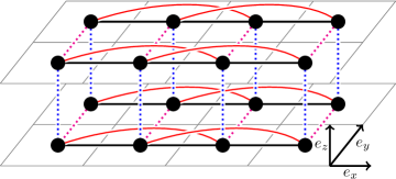
Figure 1: (Color online) Sketch of the considered model of coupled frustrated spin chains: $J_{1}$ - NN in-chain coupling (solid black), $J_{2}$ – NNN in-chain coupling (solid red), $J_{\perp,y}$ – NN inter-chain coupling in $y$-direction (dotted magenta), $J_{\perp,z}$ – NN inter-chain coupling in $z$-direction (dotted blue).

For the classical model (1) in $D=1$ (i.e., $s\rightarrow\infty$ and $J_{\perp,y}=J_{\perp,z}=0$) the critical strength of frustration, where the FM GS breaks down, is $J_{2}^{c,clas}=|J_{1}|/4$, which is also the quantum-critical point $J_{2}^{c}$ for the spin-$1/2$ model. bader For $J_{2}<J_{2}^{c}$ the GS is FM, whereas for $J_{2}>J_{2}^{c}$ the GS is a quantum spin singlet with incommensurate spiral correlations. bader ; hamada ; DKO97 ; krivnov2007 On the classical level, the spiral phase does not depend on the IC couplings $J_{\perp,y}$, or $J_{\perp,z}$ respectively, whereas for the quantum model the spiral phase does depend on the IC coupling, see, e.g., Refs. zinke2009, and Du2016, .

In the present paper we will focus on the parameter region of weak frustration $J_{2}<J^{c}_{2}$. Although, for those values of $J_{2}$ the GS is FM (i.e. it is a classical state without quantum fluctuations), the frustrating NNN bond $J_{2}$ may influence the thermodynamics substantially, in particular in the vicinity of the zero-temperature transition, i.e., at $J_{2}\lesssim J^{c}_{2}$. RGMchainfrusferro ; RGMchainarbitraryspin ; RGM2Dj1j2frusferro ; bcc_rgm_j1j2 ; Katanin2

We mention here that the case of coupled AFM spin-$1/2$ Heisenberg chains is well studied, see, e.g., Refs. HJSchulz, ; Irkhin, ; Bocquet, ; Zvyagin, . Since in this case the GS of the isolated chain is of quantum nature and does not exhibit magnetic long-range order the behavior for small IC is different to our case of FM chains.

It is appropriate to notice that in real edge-shared cuprates often the inter-chain coupling is more sophisticated than that we consider in our paper. Moreover, there is a large variety in the topology of the IC, see, e.g., Ref. prb2015, . However, the simplest case of a perpendicular IC $J_{\perp}$ corresponds, e.g., to LiVCuO₄ and Li(Na)Cu₂O₂.gippius2004 ; rosner ; enderle2005 ; buettgen2007 Furthermore, we note that most of these compounds exhibit spiral spin-spin correlations along the chain direction, i.e., the frustration exceeds $J^{c}_{2}$. Hence, there is no direct relation of our results to those compounds with $J_{2}>J^{c}_{2}$, and the focus here is on the general question for the crossover from a purely 1D $J_{1}-J_{2}$ ferromagnet to a quasi-1D and finally to a 3D system.

II Rotation-invariant Green’s function method (RGM)

The RGM has been widely applied to frustrated quantum spin systems. RGMchainfrusferro ; RGMchainarbitraryspin ; RGMchainfrusferromagnet ; barabanov94 ; ihle2001 ; canals2002 ; prb2004 ; schmal2006 ; RGMmoritzcollinearstripe ; RGM2Dj1j2frusferro ; bcc_rgm_j1j2 Therefore, we illustrate here only some basic relevant features of the method. At that we follow Refs. RGMchainfrusferro, and bcc_rgm_j1j2, . The retarded two-time Green’s function in momentum space $\langle\langle S_{\mathbf{q}}^{+};S_{-\mathbf{q}}^{-}\rangle\rangle_{\omega}=-\chi_{\mathbf{q}}^{+-}(\omega)$ determines the spin-spin correlation functions and the thermodynamic quantities. The equation of motion in the second order using spin rotational symmetry, i.e., $\langle S_{i}^{z}\rangle=0$, is expressed as $\omega^{2}\langle\langle S_{\mathbf{q}}^{+};S_{-\mathbf{q}}^{-}\rangle\rangle_{\omega}=M_{\mathbf{q}}+\langle\langle-\ddot{S}_{\mathbf{q}}^{+};S_{-\mathbf{q}}^{-}\rangle\rangle_{\omega}$ with $M_{\mathbf{q}}=\left\langle\left[[S_{\mathbf{q}}^{+},H],S_{-\mathbf{q}}^{-}\right]\right\rangle$ and $-\ddot{S}_{\mathbf{q}}^{+}=\left[[S_{\mathbf{q}}^{+},H],H\right]$. For our model (1) the moment $M_{\bf{q}}$ is given by

$$M_{\bf{q}} = 4J_{1}c_{100}(\cos(q_{x})-1)+4J_{2}c_{200}(\cos(2q_{x})-1)$$

$$+ 4J_{\perp,y}c_{010}(\cos(q_{y})-1)+4J_{\perp,z}c_{001}(\cos(q_{z})-1),$$

where $c_{hkl}\equiv c_{\bm{R}}=\langle S_{\bm{0}}^{+}S_{\bm{R}}^{-}\rangle=2\langle{\bf S}_{\bm{0}}{\bf S}_{\bm{R}}\rangle/3$, $\bm{R}=h\bm{a}_{1}+k\bm{a}_{2}+l\bm{a}_{3}$, ($\bm{a}_{j}$ are the cartesian unit vectors). For the second derivative $-\ddot{S}_{i}^{+}$ we apply the decoupling scheme in real space kondoyamaji ; ShiTak1991 ; RhoScal94 ; SSI94 ; barabanov94 ; winterfeldt97 ; ihle2001

$$S_{i}^{+}S_{j}^{+}S_{k}^{-} =\alpha_{i,k}\langle S_{i}^{+}S_{k}^{-}\rangle S_{j}^{+}+\alpha_{j,k}\langle S_{j}^{+}S_{k}^{-}\rangle S_{i}^{+},$$ (3)

where $i\neq j\neq k\neq i$ and the quantities $\alpha_{i,j}$ are vertex parameters introduced to improve the decoupling approximation. In the minimal version of the RGM we consider as many vertex parameters as independent conditions for them can be found, i.e., we have $\alpha_{x}$, $\alpha_{y}$, and $\alpha_{z}$, related to in-chain ($\alpha_{x}$) and inter-chain correlators ($\alpha_{y}$ and $\alpha_{z}$).

By using the operator identity $\bm{S}_{i}^{2}=S_{i}^{+}S_{i}^{-}-S_{i}^{z}+(S_{i}^{z})^{2}$ we get the sum rule

$$\langle S_{j}^{-}S_{j}^{+}\rangle=\langle S_{j}^{+}S_{j}^{-}\rangle=\frac{1}{2},$$ (4)

where $\langle S_{j}^{z}\rangle=0$ was used. The decoupling scheme (3) leads to the equation $-\ddot{S}_{\mathbf{q}}^{+}=\omega_{\mathbf{q}}^{2}{S}_{\mathbf{q}}^{+}$ in momentum space. Then we get

$$\chi^{+-}_{\mathbf{q}}(\omega)=-\langle\langle S_{\mathbf{q}}^{+};S_{-\mathbf{q}}^{-}\rangle\rangle_{\omega}=\frac{M_{\mathbf{q}}}{\omega_{\mathbf{q}}^{2}-\omega^{2}}$$ (5)

with the dispersion relation

$$\omega_{\bf{q}}^{2} = \sum_{n}J_{n}^{2}(1-\text{cos}(\mathbf{r}_{n}\mathbf{q}))(1+2p_{2\mathbf{r}_{n}}-2p_{\mathbf{r}_{n}})$$

$$- \sum_{n}J_{n}^{2}(1-\text{cos}(\mathbf{r}_{n}\mathbf{q}))(4\text{cos}(\mathbf{r}_{n}\mathbf{q})p_{\mathbf{r}_{n}})$$

$$+ \sum_{n\neq m}J_{n}J_{m}(1-\textrm{cos}(\mathbf{r}_{n}\mathbf{q}))\left(4p_{\mathbf{r}_{n}+\mathbf{r}_{m}}-4\textrm{cos}(\mathbf{r}_{m}\mathbf{q})p_{\mathbf{r}_{n}}\right)$$

$$+ 2J_{1}J_{2}\left(1-\textrm{cos}(q_{x})\right)\left(3+2\textrm{cos}(q_{x})\right)\left(p_{(1,0,0)}-p_{(3,0,0)}\right),$$

where the following abbreviations are used:

$$J_{3}=J_{\perp,y},\;\;J_{4}=J_{\perp,z},\hskip 145.10922pt$$

$$r_{1}=(1,0,0),\;r_{2}=(2,0,0),\;r_{3}=(0,1,0),\;r_{4}=(0,0,1),$$

$$p_{(n,0,0)}=\alpha_{x}c_{n00},\;\;p_{(m,n,0)}=\alpha_{y}c_{mn0},\hskip 76.82234pt$$

$$p_{(m,0,n)}=\alpha_{z}c_{m0n},\;\;p_{(0,n,m)}=(\alpha_{y}+\alpha_{z})c_{0nm}/2\;.\hskip 31.86694pt$$ (7)

Moreover, lattice symmetry is exploited to reduce the number of non-equivalent correlators entering Eq. (II). Expanding $\omega_{\bf{q}}$ around $\mathbf{q}=\Gamma=(0,0,0)$ we find $\frac{\partial\omega_{\mathbf{q}}}{\partial q_{i}}|_{\mathbf{q}=\mathbf{0}}=v_{i}$ and $\frac{\partial^{2}\omega_{\mathbf{q}}}{2\partial q_{i}^{2}}|_{\mathbf{q}=\mathbf{0}}=\rho_{i}$. Here the quantities $v_{i}$, $i=x,y,z$, are the spin-wave velocities relevant for AFM $J_{\perp}$, and $\rho_{i}$, $i=x,y,z$, are the spin-stiffness parameters relevant for FM $J_{\perp}$. The corresponding equations for the spin-wave velocities $v_{i}$ (Eqs. (16),(17) and (18)) and for the spin stiffnesses $\rho_{i}$ (Eqs. (19),(20) and (21)) are provided in the Appendix.

The uniform static spin susceptibility is obtained via $\chi_{0}=\lim_{{\mathbf{q}}\to{\mathbf{0}}}\chi_{\bf{q}}$, $\chi_{\bf{q}}=\chi_{\bf{q}}(\omega=0)=\chi^{+-}_{\bf{q}}(\omega=0)/2$. The explicit expression for $\chi_{0}$ is given in the Appendix, see, Eqs. (A), (A) (12), and (13). (Note that finally Eqs. (A), (A) and (12) yield $\chi_{0}=\chi_{0}^{(1)}=\chi_{0}^{(2)}=\chi_{0}^{(3)}$, because of the isotropy constraint, see below.) The correlation functions $c_{\bm{R}}=\frac{1}{N}\sum_{\mathbf{q}}c_{\mathbf{q}}\text{e}^{i\bm{qR}}$ are given by the spectral theorem,Tya67

$$c_{\mathbf{q}}=\langle S_{\mathbf{q}}^{+}S_{-\mathbf{q}}^{-}\rangle=\frac{M_{\mathbf{q}}}{2\omega_{\mathbf{q}}}[1+2n(\omega_{\mathbf{q}})],$$ (8)

where $n(\omega)=(\text{e}^{\omega/T}-1)^{-1}$ is the Bose-Einstein distribution function. In the long-range ordered phase the correlation function $c_{\bm{R}}$ is written as ShiTak1991 ; winterfeldt97 ; junger2009 ; RGMmoritzcollinearstripe

$$c_{\bm{R}}=\frac{1}{N}\sum_{\mathbf{q}\neq\mathbf{Q}}c_{\mathbf{q}}\text{e}^{i\bm{qR}}+\text{e}^{i\bm{QR}}C_{\mathbf{Q}},$$ (9)

where $c_{\mathbf{q}}$ is given by Eq. (8). The condensation term $C_{\mathbf{Q}}$, i.e. the long-range part of the correlation functions, is associated with the magnetic wave vector $\mathbf{Q}$, which describes the magnetically long-range ordered phase. Depending on the sign of $J_{\perp,y}$ and $J_{\perp,z}$ the magnetic wave vector is $\mathbf{Q}=(0,Q_{y},Q_{z})$, where $Q_{y}=0$ ($Q_{z}=0$) for FM $J_{\perp,y}<0$ ($J_{\perp,z}<0$) and $Q_{y}=\pi$ ($Q_{z}=\pi$) for AFM $J_{\perp,y}>0$ ($J_{\perp,z}>0$). The order parameter, i.e. the corresponding (sublattice) magnetization $M$, is connected with the condensation term by the formula $M=\sqrt{3C_{\mathbf{Q}}/2}$. The magnetic correlation length $\xi_{\mathbf{Q}}$ in the paramagnetic regime ($T>T_{c}$) is obtained by expanding the static susceptibility $\chi_{\mathbf{q}}$ around the magnetic wave-vector $\mathbf{Q}$, i.e. $\chi_{\mathbf{q}}\sim\chi_{\mathbf{Q}}/(1+\xi_{\mathbf{Q}}^{2}(\mathbf{Q-q})^{2})$, see, e.g., Refs. winterfeldt97, ; RGMquasi2Dvskagomelattice, ; RGMSgg1anisotropy, ; RGMmoritzcollinearstripe, .

Finally we have to make sure that as many equations are provided as unknown quantities are given. Obviously the inverse Fourier transformation of Eq. (8) yields an equation for each spatial spin-spin correlation function appearing in the system of coupled equations that has to be solved numerically. Three more equations are required to determine the vertex parameters $\alpha_{x}$, $\alpha_{y}$ and $\alpha_{z}$. One equation is provided by the sum rule Eq. (4), and the remaining two equations are obtained by the isotropy constraint, see , e.g., Refs. RGMquasi2Dvskagomelattice, ; RGMSgg1anisotropy, ; RGMmoritzcollinearstripe, , i.e. the static susceptibility $\chi_{\mathbf{q}}$ has to be isotropic in the limit $\mathbf{q}\rightarrow\mathbf{0}$: $\lim_{q_{z}\to 0}\chi(q_{x}=0,q_{y}=0,q_{z})=\chi_{0}^{(1)}=\lim_{q_{y}\to 0}\chi(q_{x}=0,q_{y},q_{z}=0)=\chi_{0}^{(2)}$ and $\lim_{q_{z}\to 0}\chi(q_{x}=0,q_{y}=0,q_{z})=\lim_{q_{x}\to 0}\chi(q_{x},q_{y}=0,q_{z}=0)=\chi_{0}^{(3)}$, where analytical expressions for $\chi_{0}^{(i)}$, $i=1,2,3$, are given in the Appendix, see Eqs. (A) - (13). Moreover, in the magnetically ordered phase we use the divergence of the static susceptibility $\chi^{-1}_{\bf{Q}}=0$ at the corresponding magnetic wave-vector $\mathbf{Q}$ to calculate the condensation term $C_{\bf{Q}}$, see e.g. Refs. junger2009, ; RGMmoritzcollinearstripe, ; bcc_rgm_j1j2, . For antiferromagnetic IC ($J_{\perp,y}>0$ and $J_{\perp,z}>0$), for instance, the relevant staggered susceptibility $\chi_{(0,\pi,\pi)}$ is given by Eq. (14), and the condition for long-range order reads as $\Delta_{(0,\pi,\pi)}=0$, see Eq. (15), which corresponds to the vanishing of the gap in $\omega_{\mathbf{q}}$ at ${\mathbf{q}}={\mathbf{Q}}={(0,\pi,\pi)}$.

III Results

Although, the two ICs $J_{\perp,y}$ and $J_{\perp,z}$ are treated as independent variables in our theory, in what follows we will consider the case with identical ICs in $y$- and $z$-direction, i.e. $J_{\perp,y}=J_{\perp,z}=J_{\perp}$. Moreover, we set $J_{1}=-1$ and we focus on weak and moderate IC $|J_{\perp}|\leq 1$.

III.1 Zero-temperature properties

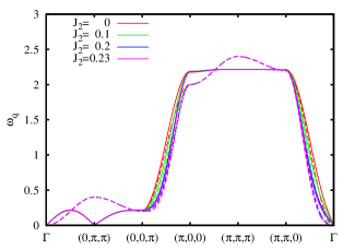
Figure 2: (Color online) Spin-wave dispersion $\omega_{\mathbf{q}}$ as a function of the wave vector $\mathbf{q}$ at zero temperature along several paths through the Brillouin Zone (dashed lines: FM $J_{\perp}=-0.1$; solid lines: AFM $J_{\perp}=0.1$). Note that in the regions $\Gamma\ldots(0,0,\pi)$ and $(\pi,0,0)\dots\Gamma$ all solid as well as all dashed lines coincide.

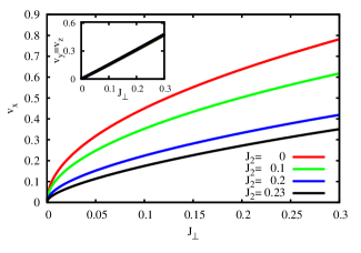
Figure 3: (Color online) GS spin-wave velocities $v_{x}$ (in-chain, main panel) and $v_{y}=v_{z}$ (inter-chain, inset) as a function of the AFM IC $J_{\perp}>0$ for different values of the frustrating NNN in-chain coupling $J_{2}$. Note that the curves of the inter-chain velocities in the inset nearly coincide.

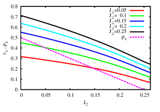
Figure 4: (Color online) GS in-chain spin-wave velocity $v_{x}$ (solid lines, AFM $J_{\perp}$) as well as the in-chain spin stiffness $\rho_{x}$ (dotted line, FM $J_{\perp}$) as a function of the frustration parameter $J_{2}$ for different values of the IC $J_{\perp}$. Note that $\rho_{x}$ given by $\rho_{x}=(\left\lvert J_{1}\right\rvert-4J_{2})/2$ is independent of $J_{\perp}$.

For ferromagnetic ICs $J_{\perp}$ and $0\leq J_{2}<-J_{1}/4$ the GS is the fully polarized long-range ordered ferromagnetic state, i.e., we have $\langle S_{\mathbf{0}}S_{\mathbf{R}}\rangle=1/4$ and the total magnetization is $M=1/2$ (i.e., the condensation term is $C_{{\bf Q}^{FM}}=1/6$). The corresponding spin-wave dispersion $\omega_{\bf{q}}$ is shown in Fig. 2 (dashed lines) for $J_{\perp}=-0.1$ and various values of $J_{2}$. Obviously, the influence of $J_{2}$ on the general shape of $\omega_{\bf{q}}$ is fairly weak. At the magnetic wave-vector ${\bf q}={\bf Q}^{FM}=\bf{0}$ ($\Gamma$ point) there is a quadratic dispersion (i.e.,$\omega_{q_{i}}\propto\rho_{i}q_{i}^{2}$, with $i=x,y,z$), that is typical for ferromagnets. The stiffness parameters, see also Eqs. (19) and (20), are given by $\rho_{x}=\left\lvert J_{1}+4J_{2}\right\rvert/2$ (in-chain) and $\rho_{\gamma}=\left\lvert J_{\perp,\gamma}\right\rvert/2$ ($\gamma=y,z$, inter-chain).

In the case of AFM ICs $J_{\perp}>0$ the GS is of quantum nature. The corresponding magnetic wave-vector is $Q^{AFM}=(0,\pi,\pi)$. The dispersion is linear for small values of $|\bf{q}|$, i.e., the low-lying excitations are determined by the spin-wave velocities $v_{x}$ and $v_{y}=v_{z}$. Again, the influence of $J_{2}$ on the general shape of $\omega_{\bf{q}}$ is fairly weak, cf. the solid lines in Fig. 2. Since several GS correlation functions enter the expressions for the spin-wave velocities, cf. Eqs. (16) and  (17), no simple expressions can be given. However, it can be seen from these equations that $v_{x}$, $v_{y}$, and $v_{z}$ are vanishing in the limit $J_{\perp}\rightarrow 0^{+}$ as expected. We show the spin-wave velocities in Figs. 3 and  4. Obviously, the inter-chain spin-wave velocities are almost linear functions in $J_{\perp}$, i.e. $v_{\gamma}\sim aJ_{\perp}$, $\gamma=y,z$, and their dependence on the frustration parameter $J_{2}$ is weak, cf. the inset of Fig. 3. The prefactor $a$ varies between $a=1.57$ at $J_{2}=0$ and $a=1.60$ at $J_{2}=0.23$. On the other hand, the in-chain spin-wave velocity $v_{x}$ exhibits a square-root like dependence on $J_{\perp}$, cf. the main panel of Fig. 3. The influence of the in-chain frustration $J_{2}$ on $v_{x}$ (relevant for AFM $J_{\perp}$) and $\rho_{x}$ (relevant for FM $J_{\perp}$) is shown in Fig. 4.

The main effect of the frustration consists in a softening of the long-wavelength excitations, i.e. $v_{x}$ and $\rho_{x}$ decrease with growing $J_{2}$, where $v_{x}$ depends on $J_{\perp}$ and $\rho_{x}$ is independent of $J_{\perp}$. However, in contrast to $\rho_{x}$ the spin-wave velocity $v_{x}$ remains finite at the transition point $J^{c}_{2}$, as it is known, e.g., for the square-lattice $J_{1}-J_{2}$ model.nonlin_sigma ; Schulz ; ED40

Next we consider the magnetic order parameter $M$ for AFM IC, which is related to the condensation term $C_{\mathbf{Q}}$ at the magnetic wave vector $\mathbf{Q}=\mathbf{Q}^{AFM}=(0,\pi,\pi)$, cf. Sec. II. We show the dependence of $M$ on the IC in Fig. 5. Starting from $M=1/2$ at $J_{\perp}=0$ the order parameter decreases monotonously with increasing $J_{\perp}$ indicating the role of quantum fluctuations introduced to the system by AFM $J_{\perp}$. Moreover, it can be seen from Fig. 5 that the larger $J_{2}$ the steeper the decrease of $M$ with growing $J_{\perp}$. A more explicit view on the influence of frustration $J_{2}$ on $M$ is presented in Fig. 6. As can be expected already from Fig. 5, we have a monotonic decrease of the order parameter with increasing $J_{2}$, i.e. naturally frustration acts against magnetic ordering. The breakdown of the $Q^{AFM}=(0,\pi,\pi)$ long-range order at a critical value $J_{2}^{c}$ is indicated by a steep downturn of $M$. A particular feature is the slight shift of the transition point $J_{2}^{c}$ beyond the critical point of isolated chains, $J_{2}^{c}=1/4$, see Fig. 6. Thus we get $J_{2}^{c}\approx 0.256$ for $J_{\perp}=0.1$ and $J_{2}^{c}\approx 0.258$ for $J_{\perp}=0.2$. Such a shift of $J_{2}^{c}$ to higher values was previously also reported for the two-dimensional case, i.e. $J_{\perp,y}>0$ and $J_{\perp,z}=0$, see Ref. zinke2009, .

Finally we briefly discuss the uniform static susceptibility $\chi_{0}$ for AFM $J_{\perp}$, see Eq. (A). Consistently, $\chi_{0}$ diverges at $J_{\perp}=0$. The inverse uniform susceptibility, $1/\chi_{0}$, as a function of $J_{\perp}$ is shown in the inset of Fig. 5. Obviously, $1/\chi_{0}$ is an almost linear function of $J_{\perp}$, and the dependence on the frustration parameter $J_{2}$ is weak. A fit according to $\chi_{0}^{-1}=aJ_{\perp}$ of the data shown in Fig. 5 yields $a=12.25$, $12.35$, $12.56$, and $12.69$ for $J_{2}=0$, $0.1$, $0.2$, and $0.23$, respectively.

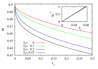
Figure 5: (Color online) GS magnetic order parameter $M$ (main panel) and inverse uniform susceptibility $\chi_{0}^{-1}$ (inset) as a function of the AFM IC $J_{\perp}$ for different values of the frustrating NNN in-chain coupling $J_{2}$. Note that the curves of the inverse uniform susceptibility in the inset practically coincide.

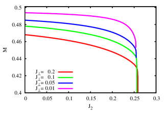
Figure 6: (Color online) GS magnetic order parameter $M$ as a function of the frustrating NNN in-chain coupling $J_{2}$ for different values of AFM IC $J_{\perp}>0$.

III.2 Finite-temperature properties

For the very existence of magnetic long-range order in an isotropic Heisenberg spin system at finite temperatures a 3D exchange pattern is necessary,mermin66 i.e., finite ICs, $J_{\perp,y}\neq 0$ and $J_{\perp,z}\neq 0$ are required. Again in this section we consider the special case of $J_{\perp,y}=J_{\perp,z}=J_{\perp}$. We mention that RGM data for the physical quantities at arbitrary sets of $J_{2}$, $J_{\perp,y}$ and $J_{\perp,z}$ are available upon request.

III.2.1 Order parameters, critical temperatures and spin-spin correlation functions

In Fig. 7 we show some typical temperature profiles of the order parameter calculated for $J_{\perp}=\pm 0.1$ and various values of frustrating $J_{2}$. In accordance with previous studies on quasi-two-dimensional unfrustrated spin systems oitmaa2004 ; junger2009 we find that for $J_{2}=0$ the transition temperature $T_{c}$ is larger if AFM interactions are present. If $J_{2}>0$ the transition temperature is a result of a subtle interplay of frustration $J_{2}$ and IC $J_{\perp}$, since these parameters influence $T_{c}$ in an opposite direction. An illustration of the influence of $J_{2}$ and $J_{\perp}$ on $T_{c}$ is provided in Figs. 8 and 9. From Fig. 8 (main panel) it is obvious that the slope of the $T_{c}(J_{\perp})$ curve is largest at $J_{\perp}\sim 0$. Moreover, following the trend observed at $J_{2}=0$ we find that $T_{c}$ for AFM $J_{\perp}\gtrsim 0.1$ is larger than $T_{c}$ for corresponding FM IC irrespective of the strength of frustration. As we can see from Fig. 9 (main panel) the reduction of $T_{c}$ due to frustration is moderate as long as $J_{2}$ is not too close to the critical strength of frustration $J_{2}^{c}$, where the FM GS ordering along the chains breaks down. Only as approaching $J_{2}^{c}$ there is a drastic downturn of $T_{c}$, cf. also Ref. bcc_rgm_j1j2, .

It is useful to compare the calculated critical temperatures with the Curie-Weiss temperature $\Theta_{CW}$ given for the model at hand by $\Theta_{CW}=-\frac{1}{2}(J_{1}+J_{2}+J_{\perp,y}+J_{\perp,z})$, where $J_{1}=-1$ (FM) and $J_{2}\geq 0$ (AFM). The absolute value of $\Theta_{CW}$ can be considered as a measure for the strength of the exchange interactions. Thus, in ordinary unfrustrated 3D magnets it determines the magnitude of the critical temperature $T_{c}$. The ratio $f=|\Theta_{CW}/T_{c}|$ is often considered as the degree of frustration see, e.g., Refs. Balents, ; Lang2016, ; Hallas2016, . In conventional 3D ferro- and antiferromagnets this ratio is of the order of unity, whereas $f\gtrsim 5$ indicates a suppression of magnetic ordering. One may expect that also for unfrustrated or weakly frustrated quasi-2D (quasi-1D) systems in the limit of small inter-layer (inter-chain) coupling the parameter $f$ can be large. We show $f$ in the insets of Figs. 8 and 9. Indeed from Fig. 8 we notice that for $|J_{\perp}|<0.05$ the ratio $f$ increases drastically. Thus, even for $J_{2}=0$ we find $f>5$ at $J_{\perp}<0.022$. The role of the frustrating coupling $J_{2}$ is illustrated in Fig. 9. It is obvious, that the influence of $J_{2}$ is weak in a wide range of $J_{2}$ values. Only as approaching the critical frustration $J_{2}^{c}$ there is a tremendous increase of $f$ beyond $f>10$. We may conclude that the magnitude of the frustration parameter is a result of a subtle interplay of $J_{\perp}$ and $J_{2}$, and, a large value of $f$ does not unambiguously indicate frustration.

The order-disorder transition is also evident in the spin-spin correlation functions $\langle{\bf S}_{0}{\bf S}_{\bf R}\rangle$, see Figs. 10 and 11. Thus, for small $|J_{\perp}|$ the inter-chain correlations $\langle{\bf S}_{0}{\bf S}_{\bf{R}}\rangle$, ${\bf R}=(0,0,n)$, become very small at $T>T_{c}$, whereas the correlations along the chain direction, $\langle{\bf S}_{0}{\bf S}_{\bf{R}}\rangle$, ${\bf R}=(n,0,0)$, remain pretty large at $T\gtrsim T_{c}$ indicating the magnetic short-range order along the chains in the paramagnetic phase. The effect of in-chain frustration $J_{2}$ is also visible by comparing the green lines in Figs. 10 and 11.

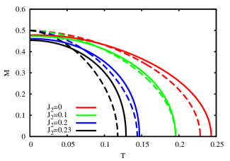
Figure 7: (Color online) Temperature dependence of the magnetic order parameter $M$ for AFM $J_{\perp}=+0.1$ (solid lines) and FM $J_{\perp}=-0.1$ (dashed lines) and various values of the frustrating in-chain coupling $J_{2}$.

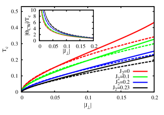
Figure 8: (Color online) Main panel: Critical temperature $T_{c}$ as a function of the IC $J_{\perp}$ (FM - dashed; AFM - solid) for several values of the frustrating in-chain coupling $J_{2}>0$. Inset: Ratio $f=|\Theta_{CW}/T_{c}|$ of the Curie-Weiss temperature $\Theta_{CW}=-\frac{1}{2}(J_{1}+J_{2}+2J_{\perp})$ and the critical temperature $T_{c}$.

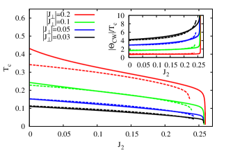
Figure 9: (Color online) Main panel: Critical temperature $T_{c}$ as a function of the frustrating in-chain coupling $J_{2}>0$ for several values of the IC $J_{\perp}$ (FM - dashed; AFM - solid). Inset: Ratio $f=|\Theta_{CW}/T_{c}|$ of the Curie-Weiss temperature $\Theta_{CW}=-\frac{1}{2}(J_{1}+J_{2}+2J_{\perp})$ and the critical temperature $T_{c}$.

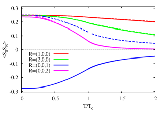
Figure 10: (Color online) Several spin-spin correlation functions as a function of the normalized temperature $T/T_{c}$ for the IC $\left\lvert J_{\perp}\right\rvert=0.1$ (AFM - solid; FM - dashed) and for $J_{2}=0$. Note that the solid and dashed lines are very close to each other (except for ${\bf R}=(0,0,1)$).

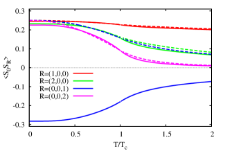
Figure 11: (Color online) Several spin-spin correlation functions as a function of the normalized temperature $T/T_{c}$ for the IC $\left\lvert J_{\perp}\right\rvert=0.1$ (AFM solid; FM dashed) and for $J_{2}=0.2$. Note that the solid and dashed lines are very close to each other (except for ${\bf R}=(0,0,1)$).

III.2.2 Correlation length and uniform static susceptibility

The correlation length, shown in Fig. 12 for the unfrustrated case, illustrates clearly the different behavior of the inter- and in-chain correlations, if $J_{\perp}$ is noticeably smaller than $J_{1}$. While the inter-chain correlation length drops down very rapidly towards one lattice spacing for $T\gtrsim T_{c}$, the in-chain correlation length remains quite large in a wider region above $T_{c}$ indicating the 1D nature of the magnetic behavior above the transition. The role of the in-chain frustration on the correlation lengths becomes evident by comparing Figs. 12 and 13. For strong frustration $J_{2}=0.2$ used for the presentation in Fig. 13 the correlation lengths form a narrow bundle, i.e., the differences between the in-chain and the inter-chain correlation lengths become much smaller compared to the case $J_{2}=0$, since the in-chain correlations on longer separations are substantially diminished by frustration.

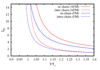
Figure 12: (Color online) Correlation length $\xi_{\mathbf{Q}}$ as a function of the normalized temperature $T/T_{c}$ for $J_{2}=0$ (FM $J_{\perp}=-0.2$ – blue; AFM $J_{\perp}=0.2$ – red; in-chain correlation length – solid, inter-chain correlation length – dashed).

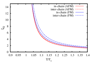
Figure 13: (Color online) Correlation length $\xi_{\mathbf{Q}}$ as a function of the normalized temperature $T/T_{c}$ for $J_{2}=0.2$ (FM $J_{\perp}=-0.2$ – blue; AFM $J_{\perp}=+0.2$ – red; in-chain correlation length – solid, inter-chain correlation length – dashed).

The temperature dependence of the susceptibility $\chi_{0}$ presented in Fig. 14 exhibits the typical behavior of antiferromagnets (main panel) and ferromagnets (left inset). The effect of frustration is evident for both FM and AFM $J_{\perp}$. For FM $J_{\perp}$ the overall shape of the curve is very similar for different $J_{2}$. However, there is a noticeable shift towards higher values of $T/T_{c}$ as increasing $J_{2}$. For AFM $J_{\perp}$ the shape of $\chi_{0}(T)$ above $T_{c}$ is affected by $J_{2}$. For the IC of $J_{\perp}=0.1$ used in Fig. 14 the critical temperature $T_{c}$ is small and there is a broad maximum in $\chi_{0}$ noticeably above $T_{c}$ related to the inter-chain antiferromagnetic correlations. By increasing $J_{2}$ the position of this maximum is shifted towards larger values of $T/T_{c}$: it is at $T/T_{c}=1.05$ for $J_{2}=0$ and at $T/T_{c}=1.23$ for $J_{2}=0.2$, see the right inset in Fig. 14. On the other hand, below $T_{c}$ the influence of $J_{2}$ on the $\chi_{0}(T/T_{c})$ curves is very weak. The influence of $J_{\perp}$ on the temperature profile of $\chi_{0}$ for AFM IC is depicted in Fig. 15. Except the influence of the IC on the critical temperature discussed in Sec. III.2.1 the strength of the AFM IC has also a strong influence on the magnitude of the uniform susceptibility at the transition point, $\chi_{0}(T_{c})$, in case of weak IC. That is related to the behavior of $\chi_{0}$ in the limit $J_{\perp}\to 0+$, where we have $T_{c}\to 0$ and $\chi_{0}(T_{c})\to\infty$. Thus, as lowering $J_{\perp}$ from moderate values to zero, $\chi_{0}(T_{c})$ increases drastically. Below $T_{c}$ the AFM IC leads to a characteristic downturn of $\chi_{0}$, cf. Fig. 15.

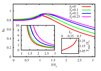
Figure 14: (Color online) Main panel: Uniform static susceptibility $\chi_{0}$ as a function of the normalized temperature $T/T_{c}$ for several values of the frustrating in-chain coupling $J_{2}$ and AFM $J_{\perp}=0.1$. Left inset: Uniform susceptibility $\chi_{0}$ as a function of the normalized temperature $T/T_{c}$ for several values of the frustrating in-chain coupling $J_{2}$ and FM $J_{\perp}=-0.1$. Right inset: Position of the maximum of the uniform susceptibility $\chi_{0}$, $T_{\mbox{max}}/T_{c}$ as a function of $J_{2}$ for AFM $J_{\perp}=0.1$.

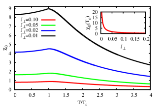
Figure 15: (Color online) Main panel: Uniform susceptibility $\chi_{0}$ as a function of the normalized temperature $T/T_{c}$ for several values of the AFM IC $J_{\perp}$ and $J_{2}=0$. Inset: The value of the uniform susceptibility at the transition temperature, $\chi_{0}(T_{c})$ as a function of the AFM IC $J_{\perp}$ for $J_{2}=0$.

III.2.3 Excitation spectrum and specific heat

Finally we consider the temperature dependence of energetic quantities such as the specific heat $C_{V}(T)$, the spin-wave velocities $v_{\gamma}$ (for AFM $J_{\perp}$) and the spin stiffnesses $\rho_{\gamma}$ (for FM $J_{\perp}$), where $\gamma=x,y,z$. Let us start with a few remarks with respect to the comparison between the RGM and the standard random-phase approximation (RPA), see, e.g., Refs. bcc_rgm_j1j2, ; heisenbergferro2d, ; Tya67, ; du, ; froebrich2006, ; bcc_RPA_2014, . The spin-wave excitation energies obtained within the framework of the RGM, see Eq. (II), show a temperature renormalization that is wavelength dependent and proportional to the correlation functions. Thus, as an example, the existence of spin-wave excitations does not imply a finite magnetization. By contrast, within the RPA, the temperature renormalization of the excitations is independent of the wavelength and proportional to the magnetization, see, e.g., Refs. Tya67, ; gasser, . Moreover, the RPA fails in describing magnetic excitations and magnetic short-range order for $T>T_{c}$, reflected, e.g., in the specific heat.heisenbergferro2d ; Tya67 ; gasser

According to the above discussion on the temperature dependence of the excitation spectrum, the RGM is appropriate to provide also information on the temperature dependence of $v_{\gamma}$ and $\rho_{\gamma}$ ($\gamma=x,y,z$), cf. Ref. bcc_rgm_j1j2, . We show the in-chain and inter-chain spin-wave velocities (relevant for AFM IC) in Figs. 16 and 17, respectively, and of the corresponding stiffnesses (relevant for FM IC) in Figs. 18 and 19, respectively. Typically, the stiffness and the spin-wave velocity decrease with increasing temperature indicating a softening of spin excitations at $T>0$, cf. Refs. Katanin2, ; Sun2006, ; Lovesey1977, ; bcc_rgm_j1j2, ; soft_swt1, ; soft_swt2, ; soft_swt3, . Interestingly, an opposite trend of the temperature influence on $v_{x}$ and $\rho_{x}$ can emerge as increasing $J_{2}$ towards the transition point $J_{2}^{c}$. That is in accordance with recent studies on other frustrated ferromagnets bcc_rgm_j1j2 ; Katanin2 and could therefore be interpreted as a signature of frustration in (anti-)ferromagnets. The temperature dependence of $\rho_{x}$ at $J_{2}=0.23$, i.e. very close to the transition point $J^{c}_{2}$, is somehow special, since it is first decreasing and then increasing with temperature.

As discussed already in Sec. III.2.1 the degree of frustration often is related to the ratio of the Curie-Weiss temperature $\Theta_{CW}$ and the transition temperature $T_{c}$, i.e. to $f=|\Theta_{CW}/T_{c}|$. We also mentioned in Sec. III.2.1 that a large value of $f$ does not unambiguously signalize frustration, since small values of $J_{\perp}$ also may lead to large values of $f$ even without any frustrating couplings. Hence, the unusual temperature dependence of the spin-wave velocity and the stiffness discussed above can be understood as another criterion to detect frustration.

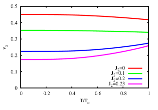
Figure 16: (Color online) In-chain spin-wave velocity $v_{x}$ as a function of the normalized temperature $T/T_{c}$ for AFM IC $J_{\perp}=0.1$ and for different values of the frustrating NNN in-chain coupling $J_{2}$.

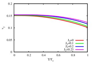
Figure 17: (Color online) Inter-chain spin-wave velocity $v_{y}=v_{z}$ as a function of the normalized temperature $T/T_{c}$ for AFM IC $J_{\perp}=0.1$ and for different values of the frustrating NNN in-chain coupling $J_{2}$.

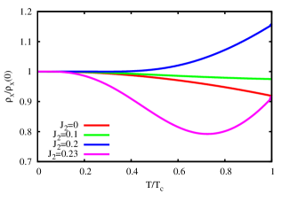
Figure 18: (Color online) In-chain spin stiffness $\rho_{x}$ scaled by its value at $T=0$ as a function of the normalized temperature $T/T_{c}$ for FM IC $J_{\perp}=-0.1$ for different values of the frustrating NNN in-chain coupling $J_{2}$.

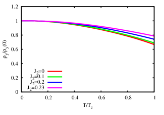
Figure 19: (Color online) Inter-chain spin stiffness $\rho_{y}=\rho_{z}$ scaled by its value at $T=0$ as a function of the normalized temperature $T/T_{c}$ for FM IC $J_{\perp}=-0.1$ for different values of the frustrating NNN in-chain coupling $J_{2}$.

The temperature dependence of the specific heat $C_{V}$ is shown in Fig. 20 for $J_{2}=0$ and two values of $J_{\perp}$. The $C_{V}(T)$ curves show the characteristic cusp-like behavior at the transition temperature $T_{c}$ indicating the second-order phase transition. For very small values of $J_{\perp}$ above the cusp a separate broad maximum emerges which is related to the in-chain spin-spin correlations, i.e., the position of this maximum is mainly determined by the in-chain exchange parameters, cf. Ref. RGMchainfrusferro, .

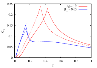
Figure 20: (Color online) Temperature dependence of the specific heat $C_{V}$ for various values of $J_{\perp}$ and $J_{2}=0$ (dashed lines: FM $J_{\perp}$; solid lines: AFM $J_{\perp}$).

IV Summary

In our paper we investigate coupled frustrated spin-$1/2$ $J_{1}$-$J_{2}$ Heisenberg chains with FM NN exchange $J_{1}$ and AFM NNN exchange $J_{2}$. We consider FM as well as AFM inter-chain couplings (ICs) $J_{\perp,y}$ and $J_{\perp,z}$ corresponding to the axis perpendicular to the chain. We focus on the regime of weak and moderate values of $J_{2}$, such that the in-chain spin-spin correlations are predominantly FM. We use the rotation-invariant Green’s function method (RGM) to calculate thermodynamic quantities, such as the (sublattice) magnetization (magnetic order parameter) $M$, the critical temperature $T_{c}$, the correlation functions $\langle{\bf S}_{0}{\bf S}_{\bf R}\rangle$, the uniform static susceptibility $\chi_{0}$, the correlation length $\xi_{\bf Q}$, the specific heat $C_{V}$, the spin stiffnesses as well as the spin-wave velocities. The RGM goes one step beyond the random-phase approximation (RPA). As a result, several shortcomings of the RPA, see, e.g., Refs. du, ; Tya67, ; gasser, ; froebrich2006, ; bcc_RPA_2014, , such as the artificial equality of the critical temperatures $T_{c}$ for FM and AFM couplings or the failure in describing the paramagnetic phase at $T>T_{c}$, can be overcome. As approaching the ground-state transition point to the helical in-chain phase at $J_{2}\sim|J_{1}|/4$, the thermodynamic properties are strongly influenced by the frustration. Thus, there is a drastic decrease of $T_{c}$ as $J_{2}\to|J_{1}|/4$. Moreover, the temperature profile of the in-chain spin stiffness $\rho_{x}$ (for FM IC) or the in-chain spin-wave velocity (for AFM IC) may exhibit an increase with $T$ instead of the ordinary decrease.

The present investigations are focused on theoretical aspects, and we consider the simplest case of perpendicular ICs. Although, there are a few materials corresponding to perpendicular ICs, e.g., LiVCuO₄ and Li(Na)Cu₂O₂ gippius2004 ; rosner ; enderle2005 ; buettgen2007 , in real magnetic $J_{1}$-$J_{2}$ compounds typically the ICs are more sophisticated than those we consider in our paper, see, e.g., Ref. prb2015, .

*

Appendix A Analytical Expressions

In this section we provide analytical expressions of the uniform susceptibility $\chi_{0}$, the staggered susceptibility $\chi_{\mathbf{Q}=(0,\pi,\pi)}$, the spin-wave stiffnesses $\rho_{i}$ and the spin-wave velocities $v_{i}$ ($i=x,y,z$), which enter the equations given in Sec. II.

Static susceptibility:

$$\lim_{q_{z}\to 0}\chi(q_{x}=0,q_{y}=0,q_{z})=\chi_{0}^{(1)}$$

$$\quad=-\frac{2c_{001}}{-4J_{1}p_{001}+4J_{1}p_{101}-4J_{\perp,y}p_{001}+4J_{\perp,y}p_{011}-6J_{\perp,z}p_{001}+2J_{\perp,z}p_{002}-4J_{2}p_{001}+4J_{2}p_{201}+J_{\perp,z}},$$ (10)

$$\lim_{q_{y}\to 0}\chi(q_{x}=0,q_{y},q_{z}=0)=\chi_{0}^{(2)}$$

$$\quad=-\frac{2c_{010}}{-4J_{1}p_{010}+4J_{1}p_{110}-6J_{\perp,y}p_{010}+2J_{\perp,y}p_{020}-4J_{\perp,z}p_{010}+4J_{\perp,z}p_{011}-4J_{2}p_{010}+4J_{2}p_{210}+J_{\perp,y}},$$ (11)

$$\lim_{q_{x}\to 0}\chi(q_{x},q_{y}=0,q_{z}=0)=\chi_{0}^{(3)}=\frac{2J_{1}c_{100}+8J_{2}c_{200}}{\Delta^{(3)}_{\mathbf{0}}},$$ (12)

$$\Delta^{(3)}_{\mathbf{0}} = J_{1}^{2}(6p_{100}-2p_{200}-1)+2J_{1}(2J_{\perp,y}(p_{100}-p_{110})+2J_{\perp,z}p_{100}-2J_{\perp,z}p_{101}-3J_{2}p_{100}+8J_{2}p_{200}-5J_{2}p_{300})$$ (13)

$$+ 4J_{2}(4(J_{\perp,y}p_{200}-J_{\perp,y}p_{210}+J_{\perp,z}p_{200}-J_{\perp,z}p_{201})+J_{2}(6p_{200}-2p_{400}-1)),$$

$$\chi_{(0,\pi,\pi)} = -\frac{2(J_{\perp,y}c_{010}+J_{\perp,z}c_{001})}{\Delta_{(0,\pi,\pi)}},$$ (14)

$$\Delta_{(0,\pi,\pi)} = 4J_{\perp,y}(-J_{1}p_{010}+J_{1}p_{110}+J_{\perp,z}(p_{001}+p_{010}+2p_{011})-J_{2}p_{010}+J_{2}p_{210})$$ (15)

$$+ J_{\perp,z}(-4J_{1}p_{001}+4J_{1}p_{101}+2J_{\perp,z}p_{001}+2J_{\perp,z}p_{002}-4J_{2}p_{001}+4J_{2}p_{201}+J_{\perp,z})$$

$$+ J_{\perp,y}^{2}(2p_{010}+2p_{020}+1).$$

Spin-wave velocities:

$$v_{x}^{2} = J_{1}^{2}\left(-3p_{100}+p_{200}+\frac{1}{2}\right)$$ (16)

$$+ J_{1}(2J_{\perp,y}(p_{110}-p_{100})-2J_{\perp,z}p_{100}+2J_{\perp,z}p_{101}+3J_{2}p_{100}-8J_{2}p_{200}+5J_{2}p_{300})$$

$$+ 2J_{2}(-4J_{\perp,y}p_{200}+4J_{\perp,y}p_{210}-4J_{\perp,z}p_{200}+4J_{\perp,z}p_{201}-6J_{2}p_{200}+2J_{2}p_{400}+J_{2}),$$

$$2v_{y}^{2}/J_{\perp,y} = -4J_{1}p_{010}+4J_{1}p_{110}-6J_{\perp,y}p_{010}+2J_{\perp,y}p_{020}-4J_{\perp,z}p_{010}$$ (17)

$$+ 4J_{\perp,z}p_{011}-4J_{2}p_{010}+4J_{2}p_{210}+J_{\perp,y},$$

$$2v_{z}^{2}/J_{\perp,z} = -4J_{1}p_{001}+4J_{1}p_{101}-4J_{\perp,y}p_{001}+4J_{\perp,y}p_{011}-6J_{\perp,z}p_{001}$$ (18)

$$+ 2J_{\perp,z}p_{002}-4J_{2}p_{001}+4J_{2}p_{201}+J_{\perp,z}.$$

Spin stiffnesses:

$$24\rho^{2}_{x} = J_{1}^{2}(30p_{100}-2p_{200}-1)+16J_{2}(4(J_{\perp,y}p_{200}-J_{\perp,y}p_{210}+J_{\perp,z}p_{200}-J_{\perp,z}p_{201})+J_{2}(30p_{200}-2p_{400}-1))$$ (19)

$$+ 2J_{1}(2J_{\perp,y}(p_{100}-p_{110})+2J_{\perp,z}p_{100}-2J_{\perp,z}p_{101}+33J_{2}p_{100}+80J_{2}p_{200}-17J_{2}p_{300}),$$

$$36\rho_{y}^{2} = -6J_{\perp,y}(J_{1}(p_{110}-p_{010})-J_{\perp,z}p_{010}+J_{\perp,z}p_{011}-J_{2}p_{010}+J_{2}p_{210})$$ (20)

$$- J_{\perp,y}^{2}(3(p_{020}-15p_{010})+\frac{3}{2}),$$

$$36\rho_{z}^{2} = -6J_{\perp,z}(J_{1}(p_{101}-p_{001})-J_{\perp,y}p_{001}+J_{\perp,y}p_{011}-J_{2}p_{001}+J_{2}p_{201})$$ (21)

$$- J_{\perp,z}^{2}(3(p_{002}-15p_{001})+\frac{3}{2}).$$

References

- (1) W. Selke, Z.f.Physik B: Condensed Matter 27, 81 (1977).
- (2) H.P. Bader and R. Schilling, Phys. Rev. B 19, 3556 (1979).
- (3) T. Hamada, J. Kane, S. Nakagawa, and Y. Natsume, J. Phys. Soc. Jpn. 57, 1891 (1988); 58, 3869 (1989).
- (4) A. V. Chubukov, Phys. Rev. B 44, 4693(R) (1991).
- (5) D.V. Dmitriev, V.Ya. Krivnov, and A.A. Ovchinnikov, Phys.Rev. B 56, 5985 (1997).
- (6) D. V. Dmitriev, V. Ya. Krivnov, and J. Richter Phys. Rev. B 75, 014424 (2007).
- (7) T. Vekua, A. Honecker, H.-J. Mikeska, and F. Heidrich-Meisner, Phys. Rev. B 76, 174420 (2007).
- (8) T. Hikihara, L. Kecke, T. Momoi, and A. Furusaki, Phys. Rev. B 78, 144404 (2008).
- (9) M. Härtel, J. Richter, D. Ihle, and S.-L. Drechsler, Phys. Rev. B 78, 174412 (2008).
- (10) J. Sudan, A. Lüscher, and A. M. Läuchli, Phys. Rev. B 80, 140402 (2009).
- (11) R. Zinke, S.-L. Drechsler, and J. Richter, Phys. Rev. B 79, 094425 (2009).
- (12) R. Shindou and T. Momoi, Phys. Rev. B 80, 064410 (2009).
- (13) J. Sirker, Phys. Rev. B 81, 014419 (2010).
- (14) D. V. Dmitriev and V. Ya. Krivnov, Phys. Rev. B 82, 054407 (2010).
- (15) M. E. Zhitomirsky, and H. Tsunetsugu, Europhysics Letters 92, 37001 (2010).
- (16) M. Arlego, F. Heidrich-Meisner, A. Honecker, G. Rossini, and T. Vekua, Phys. Rev. B 84, 224409 (2011).
- (17) A. Lavarelo, G. Roux, and N. Laflorencie, Phys. Rev. B 84, 144407 (2011).
- (18) M. Chen and C. D. Hu, Phys. Rev. B 84, 094433 (2011).
- (19) M. Härtel, J. Richter, D. Ihle, J. Schnack, and S.-L. Drechsler, Phys. Rev. B 84, 104411 (2011).
- (20) M. Härtel, J. Richter, and D. Ihle, Phys. Rev. B 83, 214412 (2011).
- (21) A. V. Syromyatnikov, Phys. Rev. B 86, 014423 (2012).
- (22) C. Lee, Jia Liu, M.-H. Whangbo, H.-J. Koo, R. K. Kremer, and A. Simon, Phys. Rev. B 86, 060407(R) (2012).
- (23) D. Bimla, K. Brijesh, and V. P. Ramesh , Europhysics Letters 100, 27003 (2012).
- (24) D. V. Dmitriev and V. Ya. Krivnov, Phys. Rev. B 86, 134407 (2012).
- (25) A. Smerald and N. Shannon, Phys. Rev. B 88, 184430 (2013).
- (26) M. Sato, T. Hikihara, and T. Momoi, Phys. Rev. Lett. 110, 077206 (2013).
- (27) O. A. Starykh, and L. Balents, Phys. Rev. B 89, 104407 (2014).
- (28) K. Manoranjan, P. Aslam, and G. S. Zoltán, arXiv:1507.03720 (2015).
- (29) O. Hiroaki, arXiv:1506.06891 (2015).
- (30) A. A. Gippius, E. N. Morozova, A. S. Moskvin, A. V. Zalessky, A. A. Bush, M. Baenitz, H. Rosner, and S.-L. Drechsler, Phys. Rev. B 70, 020406 (2004).
- (31) M. Enderle, C. Mukherjee, B. Fak, R.K. Kremer, J.-M. Broto, H. Rosner, S.-L. Drechsler, J. Richter, J. Málek, A. Prokofiev, W. Assmus, S. Pujol, J.-L. Raggazoni, H. Rakato, M. Rheinstädter, and H.M. Ronnow, Europhys. Lett. 70, 237 (2005).
- (32) S.-L. Drechsler, O. Volkova, A.N. Vasiliev, N. Tristan, J. Richter, M. Schmitt, H. Rosner, J. Málek, R. Klingeler, A.A. Zvyagin, and B. Büchner, Phys. Rev. Lett. 98, 077202 (2007).
- (33) S.-L. Drechsler, J. Richter, R. Kuzian, J. Málek, N. Tristan, B. Büchner, A.S. Moskvin, A.A. Gippius, A. Vasiliev, O. Volkova, A. Prokofiev, H. Rakato, J.-M. Broto, W. Schnelle, M. Schmitt, A. Ormeci, C. Loison, and H. Rosner, J. Magn. Magn. Mater. 316, 306 (2007).
- (34) N. Büttgen, H.-A. Krug von Nidda, L. E. Svistov, L. A. Prozorova, A. Prokofiev, and W. Aßmus, Phys. Rev. B 76, 014440 (2007).
- (35) S. E. Dutton, M. Kumar, M. Mourigal, Z. G. Soos, J.-J. Wen, C. L. Broholm, N. H. Andersen, Q. Huang, M. Zbiri, R. Toft-Petersen, and R. J. Cava, Phys. Rev. Lett. 108, 187206 (2012).
- (36) M. Pregelj, A. Zorko, O. Zaharko, D. Arčon, M. Komelj, A. D. Hillier, and H. Berger, Phys. Rev. Lett. 109, 227202 (2012).
- (37) A. Saúl and G. Radtke, Phys. Rev. B 89, 104414 (2014).
- (38) A. Fennell, V. Y. Pomjakushin, A. Uldry, B. Delley, B. Prevost, A. Desilets-Benoit, A. D. Bianchi, R. I. Bewley, B. R. Hansen, T. Klimczuk, R. J. Cava, and M. Kenzelmann, Phys. Rev. B 89, 224511 (2014).
- (39) K. Nawa, Y. Okamoto, A. Matsuo, K. Kindo, and Y. Kitahara, J. Phys. Soc. Jpn. 83, 103702 (2014).
- (40) N. Buttgen, K. Nawa, T. Fujita, M. Hagiwara, P. Kuhns, A. Prokofiev, A. P. Reyes, L. E. Svistov, K. Yoshimura, and M. Takigawa, Phys. Rev. B 90, 134401 (2014).
- (41) L. A. Prozorova, S. S. Sosin, L. E. Svistov, N. Buttgen, J. B. Kemper, A. P. Reyes, S. Riggs, A. Prokofiev, and O. A. Petrenko, Phys. Rev. B 91, 174410 (2015).
- (42) B. Willenberg, M. Schäpers, A.U.B. Wolter, S.-L. Drechsler, M. Reehuis, J.-U. Hoffmann, B. Büchner, A.J. Studer, K.C. Rule, B. Ouladdiaf, S.Süllow, and S. Nishimoto, Phys. Rev. Lett. 116, 047202 (2016).
- (43) F. Weickert, M. Jaime, N. Scott Harrison, B. L. Leitmäe, A. Heinmaa, I. Stern, R. Janson, O. Berger, H. Rosner, and A. A. Tsirlin, arXiv:1602.01632 (2016).
- (44) K. Caslin, R. K. Kremer, F. S. Razavi, M. Hanfland, K. Syassen, E. E. Gordon, and M.-H. Whangbo, Phys. Rev. B 93, 022301 (2016).
- (45) M. Matsuda, K. Ohoyama, and M. Ohashi, J. Phys. Soc. Jpn. 68, 269 (1999).
- (46) H. F. Fong, B. Keimer, J. W. Lynn, A. Hayashi, and R. J. Cava, Phys. Rev. B 59, 6873 (1999).
- (47) S.-L. Drechsler, J. Richter, A.A. Gippius, A. Vasiliev, A.A. Bush, A.S. Moskvin, J. Malek, Yu. Prots, W. Schnelle and H. Rosner, EPL (Europhysics Letters) 73, 83 (2006).
- (48) R. O. Kuzian, S. Nishimoto, S.-L. Drechsler, J. Malek, S. Johnston, Jeroen van den Brink, M. Schmitt, H. Rosner, M. Matsuda, K. Oka, H. Yamaguchi, and T. Ito, Phys. Rev. Lett. 109, 117207 (2012).
- (49) S. Chakravarty, B.I. Halperin, D.R. Nelson, Phys. Rev. B 39, 2344 (1989).
- (50) H.J. Schulz and T.A.L. Ziman, Europhys. Lett. 18, 355 (1992); H.J. Schulz, T.A.L. Ziman, and D. Poilblanc, J. Phys. I 6, 675 (1996).
- (51) J. Richter and J. Schulenburg, Eur. Phys. J. B 73, 117 (2010)
- (52) H. T. Ueda and K. Totsuka, Phys. Rev. B 80, 014417 (2009).
- (53) S. Nishimoto, S.-L. Drechsler, R.O. Kuzian, J. van den Brink, J. Richter, W.E.A. Lorenz, Y. Skourski, R. Klingeler, and B. Büchner, Phys. Rev. Lett. 107, 097201 (2011)
- (54) S. Nishimoto, S.-L. Drechsler, R. Kuzian, J. Richter, and J. van den Brink, Phys. Rev. B 92, 214415 (2015).
- (55) Z. Z. Du, H. M. Liu, Y. L. Xie, Q. H. Wang, and J.-M. Liu Phys. Rev. B 94, 134416 (2016).
- (56) J. Kondo and K. Yamaji, Prog. Theor. Phys. 47, 807 (1972).
- (57) E. Rhodes and S. Scales, Phys. Rev. B 8, 1994 (1973).
- (58) H. Shimahara and S. Takada, J. Phys. Soc. Jpn. 60, 2394 (1991).
- (59) F. Suzuki, N. Shibata, and C. Ishii, J. Phys. Soc. Jpn. 63, 1539 (1994).
- (60) A. F. Barabanov, and V. M. Berezovskii, J. Phys. Soc. Jpn. 63, 3974 (1994); Phys. Lett. A 186, 175 (1994); Zh. Eksp. Teor. Fiz. 106, 1156 (1994) [JETP 79, 627 (1994)].
- (61) S. Winterfeldt and D. Ihle, Phys. Rev. B 56, 5535 (1997).
- (62) L. Siurakshina, D. Ihle, and R. Hayn, Phys. Rev. B 64, 104406 (2001).
- (63) B.H. Bernhard, B. Canals, and C. Lacroix, Phys. Rev. B 66, 104424 (2002).
- (64) D. Schmalfuß, J. Richter, and D. Ihle, Phys. Rev. B 70, 184412 (2004).
- (65) I. J. Junger, D. Ihle, and J. Richter, Phys. Rev. B 72, 064454 (2005).
- (66) D. Schmalfuß, J. Richter, and D. Ihle, Phys. Rev. B 72, 224405 (2005).
- (67) D. Schmalfuß, R. Darradi, J. Richter, J. Schulenburg, and D. Ihle, Phys. Rev. Lett. 97, 157201 (2006).
- (68) M. Härtel, J. Richter, O. Götze, D. Ihle, and S.-L. Drechsler, Phys. Rev. B 87, 054412 (2013).
- (69) M. Härtel, J. Richter, D. Ihle, and S.-L. Drechsler, Phys. Rev. B 81, 174421 (2010).
- (70) P. Müller, J. Richter, A. Hauser and D. Ihle. Eur. Phys. J. B 88, 159 (2015).
- (71) A.N. Ignatenko, A. A. Katanin, and V. Yu. Irkhin, JETP Lett. 97, 209 (2013).
- (72) H.J. Schulz, Phys. Rev. Lett. 77, 2790 (1996).
- (73) V. Yu. Irkhin and A. A. Katanin Phys. Rev. B 61, 6757 (2000).
- (74) M. Bocquet, Phys. Rev. B 65, 184415 (2002).
- (75) Zvyagin, A. A., and Drechsler, S.-L., Phys. Rev. B 78, 014429 (2008).
- (76) J. Richter, P. Müller, A. Lohmann, and H.-J. Schmidt, Physics Procedia 75, 813 (2015).
- (77) N.D. Mermin and H. Wagner, Phys. Rev. Lett. 17, 1133, (1966).
- (78) J. Oitmaa and Weihong Zheng, J. Phys.: Condens. Matter 16, 8653 (2004).
- (79) I. Juhász Junger, D. Ihle, and J. Richter, Phys. Rev. B 80, 064425 (2009)
- (80) S. V. Tyablikov, Methods in the Quantum Theory of Magnetism (Plenum, New York, 1967).
- (81) W. Gasser, E.Heiner, and K. Elk, Greensche Funktionen in Festkörper- und Vielteilchenphysik. WILEY-VCH, 2001.
- (82) L. Balents, Nature 464, 199 (2010).
- (83) A. G. Mihailov, A. Mailman, A. Assoud, C. M. Robertson, B. Wolf, M. Lang, and R. T. Oakley J.Am.Chem.Soc. 138, 10738 (2016).
- (84) A. M. Hallas, A. Z. Sharma, Y. Cai, T. J. Munsie, M. N. Wilson, M. Tachibana, C. R. Wiebe, and G. M. Luke, arXiv:1607.08657.
- (85) A. Du and G.Z. Wei, J. Magn. Magn. Mater. 137, 343 (1994).
- (86) P. Froebrich and P.J. Kuntz, Physics Reports 432, 223 (2006).
- (87) I. Juhasz Junger, D. Ihle, L. Bogacz, and W. Janke, Phys. Rev. B 77, 174411 (2008).
- (88) M.R. Pantic, D.V. Kapor, S.M. Radosevic, and P. Mali, Solid State Comm. 182, 55 (2014).
- (89) S.W. Lovesey, J. Phys. C: Solid State Phys. 10, L455 (1977).
- (90) Shih-Jye Sun and Hsiu-Hau Lin, Eur. Phys. J. B 49, 403 (2006).
- (91) I.A. Fomin, ZhETF, 78, 2392 (1980) (English translation - JETP 51, 1203, (1980)).
- (92) Y.M. Bunkov, in Progress in Low Temperature Physics, Vol. 14, p. 69 ed. W.P. Halperin (North Holland, San Diego 1995).
- (93) Jin An, Chang-De Gong, and Hai-Qing Li, J. Phys.: Condens. Matter 13, 115 (2001).