A Framework for Dynamic Image Sampling Based on Supervised Learning (SLADS)

Abstract

Sparse sampling schemes have the potential to dramatically reduce image acquisition time while simultaneously reducing radiation damage to samples. However, for a sparse sampling scheme to be useful it is important that we are able to reconstruct the underlying object with sufficient clarity using the sparse measurements. In dynamic sampling, each new measurement location is selected based on information obtained from previous measurements. Therefore, dynamic sampling schemes have the potential to dramatically reduce the number of measurements needed for high fidelity reconstructions. However, most existing dynamic sampling methods for point-wise measurement acquisition tend to be computationally expensive and are therefore too slow for practical applications.

In this paper, we present a framework for dynamic sampling based on machine learning techniques, which we call a supervised learning approach for dynamic sampling (SLADS). In each step of SLADS, the objective is to find the pixel that maximizes the expected reduction in distortion (ERD) given previous measurements. SLADS is fast because we use a simple regression function to compute the ERD, and it is accurate because the regression function is trained using data sets that are representative of the specific application. In addition, we introduce a method to terminate dynamic sampling at a desired level of distortion, and we extended the SLADS methodology to sample groups of pixels at each step. Finally, we present results on computationally-generated synthetic data and experimentally-collected data to demonstrate a dramatic improvement over state-of-the-art static sampling methods.

I Introduction

In conventional point-wise image acquisition, an object is measured by acquiring every measurement in a rectilinear grid. However, in certain imaging techniques one high fidelity pixel measurement can take up to $0.05$ to $5$ seconds, which translates to between $3.6-364$ hours of acquisition time for an image with $512\times 512$ resolution. Examples of such imaging techniques include X-ray diffraction spectroscopy [1], high resolution electron back scatter diffraction (EBSD) microscopy[2], and Raman spectroscopy, which are of great importance in material science and chemistry

Sparse sampling offers the potential to dramatically reduce the time required to acquire an image. In sparse sampling a subset of all available measurements are acquired, and the full resolution image is reconstructed from this set of sparse measurements. In addition to reducing image acquisition time, sparse sampling also has the potential to reduce the exposure of the object/person being imaged to potentially harmful radiation. This is critically important when imaging biological samples using X-rays, electrons, or even optical photons [3, 4]. Another advantage of sparse sampling is that it reduces the amount of measurement data that must be stored.

However, for a sparse sampling method to be useful, it is critical that the reconstruction made from the sparse set of samples allows for accurate reconstruction of the underlying object. Therefore, the selection of sampling locations becomes critically important. All methods that researchers have proposed for sparse sampling can broadly be sorted into two primary categories: static and dynamic.

Static sampling refers to any method that collects measurements in a predetermined order. Random sampling strategies such as in [5], low-discrepancy sampling [6] and uniformly spaced sparse sampling methods [7] are examples of static sparse sampling schemes. Static sampling methods can also be based on a model of the object being sampled such as in [8, 9]. In these methods knowledge of the object geometry and sparsity are used to pre-determine the measurement locations.

Alternatively, dynamic sampling refers to any method that adaptively determines the next measurement location based on information obtained from previous measurements. Dynamic sampling has the potential to produce a high fidelity image with fewer measurements because of the information available from previous measurements. Intuitively, the previous measurements provide a great deal of information about the best location for future measurements.

Over the years, a wide variety of dynamic sampling methods have been proposed for many different applications. We categorize these dynamic sampling methods into three primary categories — dynamic compressive sensing methods where measurements are unconstrained projections, dynamic sampling methods developed for specific applications where measurements are not point-wise measurements, and dynamic sampling methods developed for single pixel measurements.

In dynamic compressive sensing methods the objective at each step is to find the measurement that reduces the entropy the most. In these methods the entropy is computed using the previous measurements and a model for the underlying data. Examples of such methods include [10, 11, 12]. However, in these methods the measurements are unconstrained projections and therefore cannot readily be generalized for point-wise sampling.

The next category of dynamic sampling (DS) methods in the literature are those developed for specific applications where the measurements are not point-wise measurements. One example is [13], where the authors modify the optimal experimental design [14] framework to incorporate dynamic measurement selection in a biochemical network. Another example is presented by Seeger et al. in [15] to select optimal K-space spiral and line measurements for magnetic resonance imaging (MRI). Then Batenburg et al. in [16] presents another example for binary computed tomography, where in each step the measurement that maximizes the information gain is selected.

There are also a few DS methods developed specifically for point-wise measurements. One example is presented in [17] by Kovačević et al. In this algorithm, an object is initially measured using a sparse rectilinear grid. Then, if the intensity of a pixel is above a certain threshold, the vicinity of that pixel is also measured. However, the threshold here is empirically determined and therefore is not robust for general applications. Another point-wise dynamic sampling method was proposed in [18]. Here, in each step the pixel which when measured reduces the posterior variance the most is selected for measurement. The posterior variance is computed using samples generated from the posterior distribution using the Metropolis-Hastings algorithm. However, Monte-Carlo methods such as the Metropolis-Hastings algorithm can be very slow for cases where the dimensions of the random vector are large. Another shortcoming of this method is that it does not account for the change of conditional variance in the full image due to a new measurement.

In this paper, we present an algorithm for point-wise dynamic sampling based on supervised learning techniques that we first presented in [19]. We call this algorithm a supervised learning approach for dynamic sampling (SLADS). In each step of the SLADS algorithm we select the pixel that maximizes the expected reduction in distortion ($ERD$) given previous measurements. We estimate the $ERD$ from previous measurements using a simple regression function that we train offline. As a result, we can compute the $ERD$ very fast during dynamic sampling. However, for our algorithm to be accurate we need to train this regression function with reduction in distortion ($RD$) values resulting from many different measurements. In certain cases, where the image sizes are large, computing sufficiently many entries for the training database can be very time consuming. To solve this problem we introduce an efficient training scheme that allows us to extract many entries for the training database with just one reconstruction. We empirically validate this approximation for small images and then detail a method to find the parameters needed for this approximation when dealing with larger images. Then we introduce a stopping condition for dynamic sampling, which allows us to stop when a desired distortion level is reached, as opposed to stopping after a predetermined number of samples are acquired. Finally we extend our algorithm to incorporate group-wise sampling so that multiple measurements can be selected in each step of the algorithm.

In the results section of this paper, we first empirically validate our approximation to the $ERD$ by performing experiments on $64\times 64$ sized computationally generated EBSD images. Then we compare SLADS with state-of-the-art static sampling methods by sampling both simulated EBSD and real SEM images. We observe that with SLADS we can compute a new sample location very quickly (in the range of $1$ - $100\ ms$), and can achieve the same reconstruction distortion as static sampling methods with dramatically fewer samples. Finally, we evaluate the performance of group-wise SLADS by comparing it to SLADS and to static sampling methods.

II Dynamic Sampling Framework

In sparse image sampling we measure only a subset of all available pixels. However, for a sparse sampling technique to be useful, the measured pixels should yield an accurate reconstruction of the underlying object. Dynamic sampling (DS) is a particular form of sparse sampling in which each new measurement is informed by all the previous pixel measurements.

To formulate the dynamic sampling problem, we first denote the unknown image formed by imaging the entire underlying object as $X\in\mathbb{R}^{N}$. We then denote the value of the pixel at location $r\in\Omega$ by $X_{r}$, where $\Omega$ is the set of all locations in the image.

Now, we assume that $k$ pixels have already been measured at a set of locations $\mathcal{S}=\{s^{(1)},\cdots,s^{(k)}\}$. We then represent the measurements and the corresponding locations as a $k\times 2$ matrix

$$Y^{(k)}=\left[\begin{array}[]{c}s^{(1)},X_{s^{(1)}}\\ \vdots\\ s^{(k)},X_{s^{(k)}}\end{array}\right]\ .$$

From these measurements, $Y^{(k)}$, we can compute an estimate of the unknown image $X$. We denote this best current estimate of the image as $\hat{X}^{(k)}$.

Now we would like to determine the next pixel location $s^{(k+1)}$ to measure. If we select a new pixel location $s$ and measure its value $X_{s}$, then we can presumably reconstruct a better estimate of $X$. We denote this improved estimate as $\hat{X}^{(k;s)}$.

Of course, our goal is to minimize the distortion between $X$ and $\hat{X}^{(k;s)}$, which we denote by the following function

$$D(X,\hat{X}^{(k;s)})=\sum_{r\in\Omega}D(X_{r},\hat{X}_{r}^{(k;s)})\ ,$$ (1)

where $D(X_{r},\hat{X}_{r}^{(k;s)})$ is some scalar measure of distortion between the two pixels $X_{r}$ and $\hat{X}_{r}^{(k;s)}$. Here, the function $D(\cdot,\cdot)$ may depend on the specific application or type of image. For example we can let $D(a,b)=|a-b|^{l}$ where $l\in\mathbb{Z^{+}}$.

In fact, minimizing this distortion is equivalent to maximizing the reduction in the distortion that occurs when we make a measurement. To do this, we define $R_{r}^{(k;s)}$ as the reduction-in-distortion at pixel location $r$ resulting from a measurement at location $s$.

$$R^{(k;s)}=D(X,\hat{X}^{(k)})-D(X,\hat{X}^{(k;s)})\ .$$ (2)

Notice that typically $R^{(k;s)}$ will be a positive quantity since we expect that the distortion should reduce when we collect additional information with new measurements. While this is typically true, in specific situations $R^{(k;s)}$ can actually be negative since a particular measurement might mislead one into increasing the distortion. Perhaps more importantly, we cannot know the value of $R^{(k;s)}$ because we do not know $X$.

Therefore, our real goal will be to minimize the expected value of $R^{(k;s)}$ given our current measurements. We define the expected reduction-in-distortion ($ERD$) as

$$\bar{R}^{(k;s)}=\mathbb{E}\left[R^{(k;s)}|Y^{(k)}\right]\ .$$ (3)

The specific goal of our greedy dynamic sampling algorithm will be to select the pixel $s$ according to the following rule.

$$s^{(k+1)}=\arg\max_{s\in\Omega}\left\{\bar{R}^{(k;s)}\right\}$$ (4)

Intuitively, equation (4) selects the next pixel to maximize the expected reduction-in-distortion given all the available information $Y^{(k)}$.

Once $s^{(k+1)}$ is determined, we then form a new measurement matrix given by

$$Y^{(k+1)}=\left[\begin{array}[]{c}Y^{(k)}\\ s^{(k+1)},X_{s^{(k+1)}}\end{array}\right]\ .$$ (5)

We repeat this process recursively until the stopping condition discussed in Section IV is achieved.

In summary, the greedy dynamic sampling algorithm is given by the following iteration.

$k\leftarrow 0$ repeat            $s^{(k+1)}=\arg\max_{s\in\Omega}\left\{\bar{R}^{(k;s)}\right\}$            $Y^{(k+1)}=\left[\begin{array}[]{c}Y^{(k)}\\ s^{(k+1)},X_{s^{(k+1)}}\end{array}\right]$            $k\leftarrow k+1$       until Desired fidelity is achieved

In Section IV, we will introduce a stopping condition that can be used to set a specific expected quality level for the reconstruction.

III Supervised Learning Approach for Dynamic Sampling (SLADS)

The challenge in implementing this greedy dynamic sampling method is accurately determining the $ERD$ function, $\bar{R}^{(k;s)}$. Our approach to solve this problem is to use supervised learning techniques to determine this function from training data.

More specifically, the supervised learning approach for dynamic sampling (SLADS) will use an off-line training approach to learn the relationship between the $ERD$ and the available measurements, $Y$, so that we can efficiently predict the $ERD$. More specifically, we would like to fit a regression function $f^{\theta}(\cdot)$, so that

$$\bar{R}^{(s)}=f^{\theta}_{s}(Y)\ .$$ (6)

Here $f^{\theta}_{s}(\cdot)$ denotes a non-linear regression function determined through supervised learning, and $\theta$ is the parameter vector that must be estimated in the learning process. Notice above that we have dropped the superscript $k$ since we would like to estimate a function that will work for any number of previously measured pixels.

Now, to estimate $f^{\theta}(\cdot)$ we must construct a training database containing multiple corresponding pairs of $(R^{(s)},Y)$. Here, $R^{(s)}=D(X,\hat{X})-D(X,\hat{X}^{(s)})$, where $\hat{X}$ is the best estimate of $X$ computed using the measurements $Y$, and $\hat{X}^{(s)}$ is the best estimate of $X$ computed using the measurements $Y$ along with an additional measurement at location $s$.

Notice that since $R^{(s)}$ is the reduction-in-distortion, it requires knowledge of the true image $X$. Since this is an off-line training procedure, $X$ is available, and the regression function, $f^{\theta}_{s}(Y)$, will compute the required conditional expectation $\bar{R}^{(s)}$. However, in order to compute $R^{(s)}$ for a single value of $s$, we must compute two full reconstructions, both $\hat{X}$ and $\hat{X}^{(s)}$. Since reconstruction can be computationally expensive, this means that creating a large database can be very computationally expensive. We will address this problem and propose a solution to it in Section III-A.

For our implementation of SLADS, the regression function $f^{\theta}_{s}\left(Y\right)$ will be a function of a row vector containing features extracted from $Y$. More specifically, at each location $s$, a $p$-dimensional feature vector $V_{s}$ will be computed using $Y$ and used as input to the regression function. The specific choices of features used in $V_{s}$ are listed in Section III-D; however, other choices are possible.

From this feature vector, we then compute the $ERD$ using a linear predictor with the following form:

$$\bar{R}^{(s)}=f^{\theta}_{s}\left(Y\right)=V_{s}\,\theta.$$ (7)

We can estimate the parameter $\theta$ by solving the following least-squares regression

$$\hat{\theta}=\arg\min_{\theta\in\mathbb{R}^{p}}\|\textbf{R}-\textbf{V}\theta\|^{2}\ ,$$ (8)

where R is an $n$-dimensional column vector formed by

$$\textbf{R}=\left[\begin{array}[]{c}R^{(s_{1})}\\ \vdots\\ R^{(s_{n})}\end{array}\right]\ ,$$ (9)

and V is given by

$$\textbf{V}=\left[\begin{array}[]{c}V_{s_{1}}\\ \vdots\\ V_{s_{n}}\end{array}\right]\ .$$ (10)

So together $(\textbf{R},\textbf{V})$ consist of $n$ training pairs, $\{(R_{s_{i}},V_{s_{i}})\}_{i=1}^{n}$, that are extracted from training data during an off-line training procedure. The parameter $\theta$ is then given by

$$\hat{\theta}=\left(\textbf{V}^{t}\textbf{V}\right)^{-1}\textbf{V}^{t}\textbf{R}\ .$$ (11)

Once $\hat{\theta}$ is estimated, we can use it to find the $ERD$ for each unmeasured pixel during dynamic sampling. Hence, we find the $k+1^{th}$ location to measure by solving

$$s^{(k+1)}=\arg\max_{s\in\Omega}\left(V^{(k)}_{s}\hat{\theta}\right)\ ,$$ (12)

where $V^{(k)}_{s}$ denotes the feature vector extracted from the measurements $Y^{(k)}$ at location $s$. It is important to note that this computation can be done very fast. The pseudo code for SLADS is shown in Figure (1).

function $Y^{(K)}$ $\leftarrow$ SLADS($Y^{(k)},\hat{\theta},k$)            $\mathcal{S}\leftarrow\left\{s^{(1)},s^{(2)},\ldots s^{(k)}\right\}$            while Stopping condition not met do                    for  $\forall s\in\left\{\Omega\setminus\mathcal{S}\right\}$ do                              Extract $V^{(k)}_{s}$                              $\bar{R}^{(k;s)}\leftarrow V^{(k)}_{s}\hat{\theta}$                         end for                    $s^{(k+1)}=\arg\underset{s\in\left\{\Omega\setminus\mathcal{S}\right\}}{\operatorname{max}}\left(\bar{R}^{(k;s)}\right)$                    $Y^{(k+1)}=\left[\begin{array}[]{c}Y^{(k)}\\ s^{(k+1)},X_{s^{(k+1)}}\end{array}\right]\$                    $\mathcal{S}\leftarrow\left\{\mathcal{S}\cup s^{(k+1)}\right\}$                    $k\leftarrow k+1$                end while            $K\leftarrow k$       end function

Figure 1: SLADS algorithm in pseudo code. The inputs to the function are the initial measurements $Y^{(k)}$, the coefficients needed to compute the $ERD$, found in training, $\hat{\theta}$, and $k$, the number of measurements. When the stopping condition is met, the function will output the selected set of measurements $Y^{(K)}$.

III-A Training for SLADS

In order to train the SLADS algorithm, we must form a large training database containing corresponding pairs of $R^{(s)}$ and $V_{s}$. To do this, we start by selecting $M$ training images denoted by $\left\{X_{1},X_{2},\ldots,X_{M}\right\}$. We also select a set of sampling densities represented by $p_{1}\%,p_{2}\%,\ldots,p_{H}\%$.

For image $X_{m}$ and each sampling density, $p_{h}\%$, we randomly select $p_{h}\%$ of all pixels in the image to represent the simulated measurement locations. Then for each of the remaining unmeasured locations, $s$, in the image $X_{m}$, we compute the pairs $(R^{(s)},V_{s})$ and save them to the training database. This process is then repeated for all the sampling densities and all the images to form a complete training database.

Figure 2 illustrates this procedure. Note that by selecting a set of increasing sampling densities, the SLADS algorithm can be trained to accurately predict the $ERD$ in conditions where the sampling density is low or high. Intuitively, by sampling a variety of images with a variety of sampling densities, the final training database is constructed to represent the behaviors that will occur as the sampling density increases when SLADS is used.

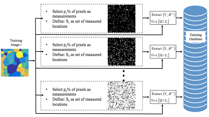
Figure 2: Illustration of how training data is extracted from one image in the training database. We first select $p_{1}\%$ of the pixels in the image and consider them as measurements $Y$. Then for all unmeasured pixel locations ($s\in\left\{\Omega\setminus\mathcal{S}_{1}\right\}$) we extract a feature vector $V_{s}$ and also compute $R^{(s)}$. We the repeat the process for when $p_{2},p_{3},\ldots$ and $p_{h}\%$ of the pixels are considered measurements. Here again $\Omega$ is the set of all locations in the training image and $\mathcal{S}_{i}$ is the set of measured locations when $p_{i}\%$ of pixels are selected as measurements. All these pairs of $\left(V_{s},R^{(s)}\right)$ are then stored in the training database.

III-B Approximating the reduction-in-distortion

While the training procedure described in Section III-A is possible, it is very computationally expensive because of the need to exactly compute the value of $R^{(s)}$. Since this computation is done in the training phase, we rewrite equation (2) without the dependence on $k$ to be

$$R^{(s)}=D(X,\hat{X})-D(X,\hat{X}^{(s)})\ ,$$ (13)

where $X$ is known in training, $\hat{X}$ is the reconstruction using the selected sample points, and $\hat{X}^{(s)}$ is the reconstruction using the selected sample points plus the value $X_{s}$. Notice that $\hat{X}^{(s)}$ must be recomputed for each new pixel $s$. This requires that a full reconstruction be computed for each entry of the training database. While this maybe possible, it typically represents a very large computational burden.

In order to reduce this computational burden, we introduce in this section a method for approximating the value of $R^{(s)}$ so that only a single reconstruction must be performed in order to evaluate $R^{(s)}$ for all pixels $s$ in an image. This dramatically reduces the computation required to build the training database.

In order to express our approximation, we first rewrite the reduction-in-distortion in the form

$$R^{(s)}=\sum_{r\in\Omega}R_{r}^{(s)},$$

where

$$R_{r}^{(s)}=D(X_{r},\hat{X}_{r})-D(X_{r},\hat{X}_{r}^{(s)}).$$

So here $R_{r}^{(s)}$ is the reduction-in-distortion at pixel $r$ due to making a measurement at pixel $s$. Using this notation, our approximation is given by

$$R_{r}^{(s)}\approx\tilde{R}_{r}^{(s)}=h_{s,r}D\left(X_{r},\hat{X}_{r}\right)\ ,$$ (14)

where

$$h_{s,r}=\exp\left\{-\frac{1}{2\sigma_{s}^{2}}\|r-s\|^{2}\right\}$$ (15)

and $\sigma_{s}$ is the distance between the pixel $s$ and the nearest previously measured pixel divided by a user selectable parameter $c$. More formally, $\sigma_{s}$ is given by

$$\sigma_{s}=\frac{\min_{t\in\mathcal{S}}\|s-t\|}{c},$$ (16)

where $\mathcal{S}$ is the set of measured locations. So this results in the final form for the approximate reduction-in-distortion given by

$$\tilde{R}^{(s)}=\sum_{r\in\Omega}h_{s,r}D\left(X_{r},\hat{X}_{r}\right)\ ,$$ (17)

where $c$ is a parameter that will be estimated for the specific problem.

In order to understand the key approximation of equation (14), notice that the reduction-in-distortion is proportional to the product of $h_{s,r}$ and $D\left(X_{r},\hat{X}_{r}\right)$. Intuitively, $h_{s,r}$ represents the weighted distance of $r$ from the location of the new measurement, $s$; and $D\left(X_{r},\hat{X}_{r}\right)$ is the initial distortion at $r$ before the measurement was made. So for example, when $r=s$, then $h_{s,r}=1$ and we have that

$$\tilde{R}_{s}^{(s)}=D\left(X_{s},\hat{X}_{s}\right)\ .$$ (18)

In this case, the reduction-in-distortion is exactly the initial distortion since the measurement is assumed to be exact. However, as $r$ becomes more distant from the pixel being measured, $s$, the reduction-in-distortion will be attenuated by the weight $h_{s,r}<1$.

Figures 3(b) and (c) illustrate the shape of $h_{s,r}$ for two different cases. In Figures 3(b), the pixel $s_{1}$ is further from the nearest measured pixel, and in Figures 3(c), the pixel $s_{2}$ is nearer. Notice that as $r$ becomes more distant from the measurement location $s$, the reduction-in-distortion becomes smaller.

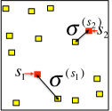
(a) Measurements

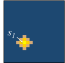
(b) $h_{s_{1},r}$

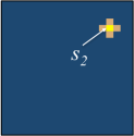
(c) $h_{s_{2},r}$

Figure 3: This figure illustrates the shape of the function $h_{s,r}$ as a function of $r$. (a) The red squares represent the two new measurement locations $s_{1}$ and $s_{2}$, and the yellow squares represent the locations of previous measurements. (b) The function $h_{s_{1},r}$ resulting from a measurement at location $s_{1}$. (c) The function $h_{s_{2},r}$ resulting from a measurement at location $s_{2}$. Notice that since $\sigma_{s_{1}}>\sigma_{s_{2}}$ then the weighting function $h_{s_{1},r}$ is wider than the function $h_{s_{2},r}$.

III-C Estimating the $c$ parameter

In this section, we present a method for estimating the parameter $c$ used in equation (17). To do this, we create a training database that contains the approximate reduction-in-distortion for a set of parameter values. More specifically, each entry of the training database has the form

$$\left(\tilde{R}^{(s;c_{1})},\tilde{R}^{(s;c_{2})},\ldots,\tilde{R}^{(s;c_{n})},V^{(s)}\right),$$

where $c\in\left\{c_{1},c_{2},\ldots c_{n}\right\}$ is a set of $n$ possible parameter values, and $\tilde{R}^{(s;c_{i})}$ is the approximate reduction-in-distortion computed using the parameter value $c_{i}$.

Using this training database, we compute the $n$ associated parameter vectors $\hat{\theta}^{(c_{i})}$, and using these parameter vectors, we apply the SLADS algorithm on $M$ images and stop each simulation when $K$ samples are taken. Then for each of these $M$ SLADS simulations, we compute the total distortion as

$$TD_{k}^{(m,c_{i})}=\frac{1}{|\Omega|}D\left(X^{(m)},\hat{X}^{(k,m,c_{i})}\right),$$ (19)

where $X^{(m)}$ is the $m^{th}$ actual image, and $\hat{X}^{(m,k,c_{i})}$ is the associated image reconstructed using the first $k$ samples and parameter value $c_{i}$. Next we compute the average total distortion over the $M$ training images given by

$$\overline{TD}_{k}^{(c_{i})}=\frac{1}{M}\displaystyle\sum\limits_{m=1}^{M}TD_{k}^{(m,c_{i})}.$$ (20)

From this, we then compute the area under the $\overline{TD}$ curve as the overall distortion metric for each $c_{i}$ given by

$$DM^{(c_{i})}=\displaystyle\sum\limits_{k=2}^{K}\frac{\overline{TD}_{k-1}^{(c_{i})}+\overline{TD}_{k}^{(c_{i})}}{2}\ ,$$ (21)

where $K$ is the total number of samples taken before stopping. The optimal parameter value, $c^{*}$, is then selected to minimize the overall distortion metric given by

$$c^{*}=\arg\min_{c\in\left\{c_{1},c_{2},\ldots c_{u}\right\}}\left\{DM^{(c)}\right\}.$$ (22)

III-D Local Descriptors in Feature Vector $V_{s}$

In our implementation, the feature vector $V_{s}$ is formed using terms constructed from the $6$ scalar descriptors $Z_{s,1},Z_{s,2},\ldots Z_{s,6}$ listed in Table I. More specifically, we take all the unique second-degree combinations formed from these descriptors to form $V_{s}$. This gives us a total of $28$ elements for the vector $V_{s}$.

$$V_{s}=[ 1,\hskip 2.84526ptZ_{s,1},\hskip 2.84526pt\ldots,\hskip 2.84526ptZ_{s,6},\hskip 2.84526ptZ_{s,1}^{2},\hskip 2.84526ptZ_{s,1}Z_{s,2},\hskip 2.84526pt\ldots,\hskip 2.84526ptZ_{s,1}Z_{s,6},$$

$$Z_{s,2}^{2},\hskip 2.84526ptZ_{s,2}Z_{s,3},\hskip 2.84526pt\ldots\hskip 2.84526pt,Z_{s,2}Z_{s,6},\ldots\hskip 2.84526pt,Z_{s,6}^{2}].$$

The first two descriptors in Table I are the gradients of the image computed from the measurement in the horizontal and vertical directions. The second two descriptors are measures of the variance for each unmeasured location. So the first four descriptors quantify the intensity variation at each unmeasured location. Then the last two descriptors quantify how densely (or sparsely) the region surrounding an unmeasured pixel is measured. In particular, the first of these descriptors is the distance from the nearest measurement to an unmeasured pixel and the second is the area fraction that is measured in a circle surrounding an unmeasured pixel.

Measures of gradients
Gradient of the reconstruction in horizontal ($x$) direction. $$Z_{s,1}=D\left(\hat{X}_{s_{x+}},\hat{X}_{s_{x-}}\right)$$ where, $s_{x+}$ and $s_{x-}$ are pixels adjacent to $s$ the horizontal direction	Gradient of the reconstruction in vertical ($y$) direction. $$Z_{s,2}=D\left(\hat{X}_{s_{y+}},\hat{X}_{s_{y-}}\right)$$ where, $s_{x+}$ and $s_{x-}$ are pixels adjacent to $s$ the horizontal direction
Measures of standard deviation
$$Z_{s,3}=\sqrt{\frac{1}{L}\displaystyle\sum\limits_{r\in\partial s}D\left(X_{r},\hat{X}_{s}\right)^{2}}$$ Here $\partial s$ is the set containing the indices of the $L$ nearest measurements to $s$.	$$Z_{s,4}=\displaystyle\sum\limits_{r\in\partial s}w_{r}^{(s)}D\left(X_{r},\hat{X}_{s}\right)$$ Here, $$w_{r}^{(s)}=\frac{\frac{1}{\|s-r\|^{2}}}{\displaystyle\sum\limits_{u\in\partial s}\frac{1}{\|s-u\|^{2}}}$$ and $\|s-r\|$ is the euclidean distance between $s$ and $r$.
Measures of density of measurements
$$Z_{s,5}=\underset{r\in\partial s}{min}\|s-r\|_{2}$$ The distance from $s$ to the closest measurement.	$$Z_{s,6}=\frac{1+A_{(s;\lambda)}}{1+A_{(s;\lambda)}^{*}}$$ Here $A_{(s;\lambda)}$ is the area of a circle $\lambda\%$ the size of the image. $A_{(s;\lambda)}^{*}$ is the measured area inside $A_{(s;\lambda)}$.

TABLE I: List of descriptors used to construct the feature vector $V_{s}$. There are three main categories of descriptors: measures of gradients, measures of standard deviation, and measures of density of measurements surrounding the pixel $s$.

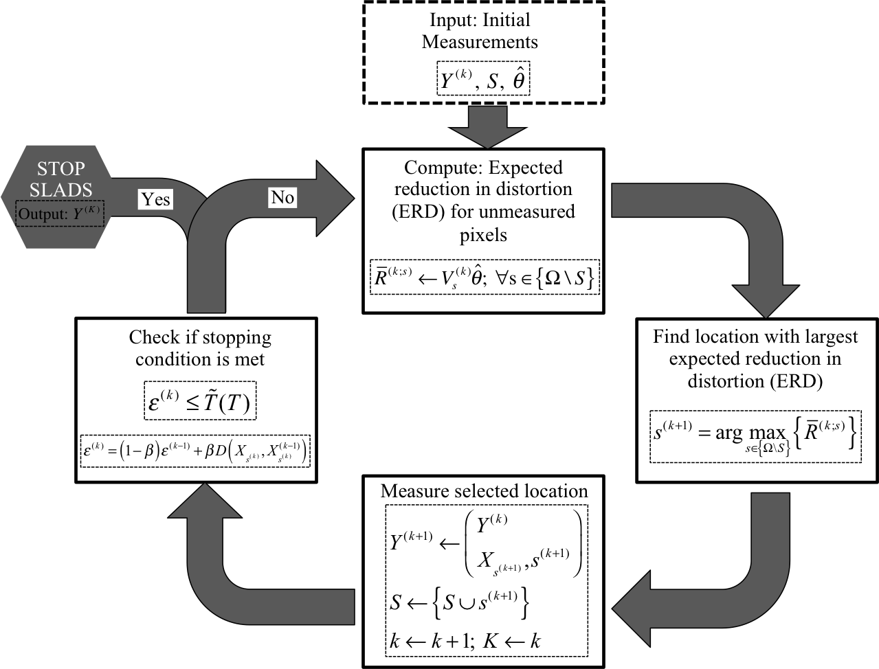
Figure 4: The SLADS algorithm as a flow diagram. The inputs to the function are the initial measurements $Y^{(k)}$, the coefficients needed to compute the $ERD$, found in training, $\hat{\theta}$, and the set $\mathcal{S}$ containing the indices of the measurements. When the stopping condition is met the function will output the selected set of measurements $Y^{(K)}$.

IV Stopping Condition for SLADS

In applications, it is often important to have a stopping criteria for terminating the SLADS sampling process. In order to define such a criteria, we first define the expected total distortion (ETD) at step $k$ by

$$\text{ETD}_{k}=\mathbb{E}\left[\frac{1}{|\Omega|}D\left(X,\hat{X}^{(k)}\right)\right]\ .$$

Notice that the expectation is necessary since the true value of $X$ is unavailable during the sampling process. Then our goal is to stop sampling when the ETD falls below a predetermined threshold.

$$\text{ETD}_{k}\leq T$$

In order to make this practical, at each step of the SLADS algorithm we compute

$$\epsilon^{(k)}=(1-\beta)\epsilon^{(k-1)}+\beta D\left(X_{s^{(k)}},\hat{X}_{s^{(k)}}^{(k-1)}\right),$$ (23)

where $k>1$, $\beta$ is a user selected parameter that determines the amount of temporal smoothing, $X_{s^{(k)}}$ is the measured value of the pixel at step $k$, and $\hat{X}_{s^{(k)}}^{(k-1)}$ is the reconstructed value of the same pixel at step $k-1$.

Intuitively, the value of $\epsilon^{(k)}$ measures the average level of distortion in the measurements. So a large value of $\epsilon^{(k)}$ indicates that more samples need to be taken, and a smaller value indicates that the reconstruction is accurate and the sampling process can be terminated. However, in typical situations, it will be the case that

$$\epsilon^{(k)}>\text{ETD}_{k}$$

because the SLADS algorithm will tend to select pixels to measure whose values have great uncertainty.

In order to compensate for this effect, we compute a function $\tilde{T}(T)$ using a look-up-table (LUT) and stop sampling when

$$\epsilon^{(k)}\leq\tilde{T}(T).$$

The function $\tilde{T}(T)$ is determined using a set of training images, $\{X_{1},\cdots,X_{M}\}$. For each image, we first determine the number of steps, $K_{m}(T)$, required to achieve the desired distortion.

$$K_{m}(T)=\min_{k}\left\{k:\frac{1}{|\Omega|}D\left(X,\hat{X}^{(k)}\right)\leq T\right\}.$$ (24)

Then we average the value of $\epsilon^{k}$ for each of the $M$ images to determine the adjusted threshold:

$$\tilde{T}(T)=\frac{1}{M}\displaystyle\sum\limits_{m=1}^{M}\epsilon_{m}^{(K_{m}(T))}.$$ (25)

Selection of the parameter $\beta$ allows the estimate of $\epsilon^{k}$ to be smoothed as a function of $k$. In practice, we have used the following formula to set $\beta$:

$$\beta=\begin{cases}0.001\left(\frac{\log_{2}\left(512^{2}\right)-\log_{2}\left(|\Omega|\right)}{2}+1\right)\quad|\Omega|\leq 512^{2}\\ 0.001\left(\frac{\log_{2}\left(|\Omega|\right)-\log_{2}\left(512^{2}\right)}{2}+1\right)^{-1}\quad|\Omega|>512^{2}\end{cases}$$

where $|\Omega|$ is the number of pixels in the image.

Figure 4 shows the SLADS algorithm as a flow diagram after the stopping condition in the previews section is incorporated.

V Group-wise SLADS

function $Y^{(K)}$ $\leftarrow$ Group-wise SLADS($Y^{(k)},\hat{\theta},k,B$)            $\mathcal{S}\leftarrow\left\{s^{(1)},s^{(1)},\ldots s^{(k)}\right\}$            while Stopping condition not met do                    for  $b=1,\ldots B$ do                              Form pseudo-measurement vector $Y^{(k+1)}_{b}$ as shown in equation (27)                              Compute pseudo-$ERD$ $\bar{R}^{(k,s^{(k+1)}_{1},s^{(k+1)}_{2}\ldots s^{(k+1)}_{b-1};s)}$ from $Y^{(k+1)}_{b}$ $\forall s\in\mathbb{S}$ using equation (28)                              $s^{(k+1)}_{b}=\arg\underset{s\in\left\{\Omega\setminus\mathcal{S}\right\}}{\operatorname{max}}\left(\bar{R}^{(k,s^{(k+1)}_{1},s^{(k+1)}_{2}\ldots s^{(k+1)}_{b-1};s)}\right)$                              $\mathcal{S}\leftarrow\left\{\mathcal{S}\cup s^{(k+1)}_{b}\right\}$                         end for          $Y^{(k+1)}=\left[\begin{array}[]{c}Y^{(k)}\\ s^{(k+1)}_{1},\hat{X}_{s^{(k+1)}_{1}}^{(k)}\\ s^{(k+1)}_{2},\hat{X}_{s^{(k+1)}_{2}}^{(k)}\\ \vdots\\ s^{(k+1)}_{b},\hat{X}_{s^{(k+1)}_{b}}^{(k)}\end{array}\right]\$                              $k\leftarrow k+1$                end while            $K\leftarrow k$       end function

Figure 5: Our proposed method for Group-wise SLADS. Here instead of just selecting $1$ measurement in each step of SLADS, as we did in Figure 1, we now select $B$ measurement locations at each step.

In this section, we introduce a group-wise SLADS approach in which $B$ measurements are made at each step of the algorithm. Group-wise SLADS may be more appropriate in applications where it is faster to measure a set of predetermined pixels in a single burst. So at the $k^{th}$ step, our goal will be to select a group of measurement positions, $\mathcal{S}^{(k+1)}=\left\{s^{(k+1)}_{1},s^{(k+1)}_{2},\ldots s^{(k+1)}_{B}\right\}$, that will yield the greatest expected reduction-in-distortion.

$$\mathcal{S}^{(k+1)}=\arg\max_{\left\{s_{1},s_{2},\ldots s_{B}\right\}\in\left\{\Omega\setminus\mathcal{S}\right\}}\left\{\bar{R}^{\left(k;s_{1},s_{2},\ldots s_{B}\right)}\right\},$$ (26)

where $\bar{R}^{\left(k;s_{1},s_{2},\ldots s_{B}\right)}$ is the expected reduction-in-distortion due to measurements $s^{(k+1)}_{1},s^{(k+1)}_{2},\ldots s^{(k+1)}_{B}$. However, solving this problem requires that we consider ${{N-|\mathcal{S}|}\choose{B}}$ different combinations of measurements.

In order to address this problem, we introduce a method in which we choose the measurements sequentially, just as we do in standard SLADS. Since group-wise SLADS requires that we make measurements in groups, we cannot make the associated measurement after each location is selected. Consequently, we cannot recompute the $ERD$ function after each location is selected, and therefore, we cannot select the best position for the next measurement. Our solution to this problem is to estimate the value at each selected location, and then we use the estimated value as if it were the true measured value.

More specifically, we first determine measurement location $s^{(k+1)}_{1}$ using equation (4), and then let $\mathcal{S}\leftarrow\left\{\mathcal{S}\cup s^{(k+1)}_{1}\right\}$. Now without measuring the pixel at $s^{(k+1)}_{1}$, we would like to find the location of the next pixel to measure, $s^{(k+1)}_{2}$. However, since $s^{(k+1)}_{1}$ has now been chosen, it is important to incorporate this information when choosing the next location $s^{(k+1)}_{2}$. In our implementation, we temporarily assume that the true value of the pixel, $X_{s^{(k+1)}_{1}}$, is given by its estimated value, $\hat{X}_{s^{(k+1)}_{1}}^{(k)}$, computed using all the measurements acquired up until the $k^{th}$ step. We will refer to $\hat{X}_{s^{(k+1)}_{1}}^{(k)}$ as a pseudo-measurement since it takes the place of a true measurement of the pixel. Now using this pseudo-measurement along with all previous real measurements, we estimate a pseudo-$ERD$ $\bar{R}^{(k,s^{(k+1)}_{1};s)}$ for all $s\in\left\{\Omega\setminus\mathcal{S}\right\}$ and from that select the next location to measure. We repeat this procedure to find all $B$ measurements.

So the procedure to find the $b^{th}$ measurement is as follows. We first construct a pseudo-measurement vector,

$$Y^{(k+1)}_{b}=\left[\begin{array}[]{c}Y^{(k)}\\ s^{(k+1)}_{1},\hat{X}_{s^{(k+1)}_{1}}^{(k)}\\ s^{(k+1)}_{2},\hat{X}_{s^{(k+1)}_{2}}^{(k)}\\ \ldots\\ s^{(k+1)}_{b-1},\hat{X}_{s^{(k+1)}_{b-1}}^{(k)}\\ \end{array}\right],\$$ (27)

where $Y^{(k+1)}_{1}=Y^{(k)}$. Then using this pseudo-measurement vector we compute the pseudo-$ERD$ for all $s\in\left\{\Omega\setminus\mathcal{S}\right\}$

$$\bar{R}^{(k,s^{(k+1)}_{1},s^{(k+1)}_{2},\ldots s^{(k+1)}_{b-1};s)}=V^{(k,s^{(k+1)}_{1},s^{(k+1)}_{2},\ldots s^{(k+1)}_{b-1})}_{s}\hat{\theta}.$$ (28)

where $V^{(k,s^{(k+1)}_{1},s^{(k+1)}_{2},\ldots s^{(k+1)}_{b-1})}_{s}$ is the feature vector that corresponds to location $s$. It is important to note that when $b=1$ the pseudo-$ERD$ is the actual $ERD$ computed using the actual measurements only. Now we find the location that maximizes the pseudo-$ERD$ by

$$s^{(k+1)}_{b}=\arg\max_{s\in\left\{\Omega\setminus\mathcal{S}\right\}}\left\{\bar{R}^{(k,s^{(k+1)}_{1},s^{(k+1)}_{2},\ldots s^{(k+1)}_{b-1};s)}\right\}.$$ (29)

Then finally we update the set of measured locations by

$$\mathcal{S}\leftarrow\left\{S\cup s^{(k+1)}_{b}\right\}.$$ (30)

Figure 5 shows a detailed illustration of the proposed group-wise SLADS method.

VI Results

In the following sections, we first validate the approximation to the $ERD$, and then we compare SLADS to alternative sampling approaches based on both real and simulated data. We then evaluate the stopping condition presented in Section IV and finally compare the group-wise SLADS method presented in Section V with SLADS. The distortion metrics and the reconstruction methods we used in these experiments are detailed in Appendices -A and -B. It is also important to note that we start all experiments by first acquiring $1\%$ of the image according to low-discrepancy sampling[6].

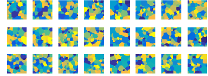
(a)

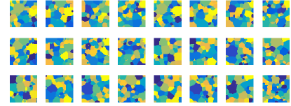
(b)

Figure 6: Images used to compute regression coefficients and perform SLADS in the experiment detailed in Section VI-A. These images have $64\times 64$ pixels each, and are synthetic EBSD image generated using the Dream.3D software. The images here are discretely labeled and the different colors correspond to different crystal orientations. In particular, (a) shows the images that were used to find the regression coefficients and (b) shows the images on which SLADS was performed.

VI-A Validating the $ERD$ Approximation

In this section, we compare the results using the true and approximate $ERD$ described in Section III-B in order to validate the efficacy of the approximation. The SLADS algorithm was trained and then tested using the synthetic EBSD images shown in Figures 6(a) and 6(b). Both sets of images were generated using the Dream.3D software [20].

The training images were constructed to have a small size of $64\times 64$ so that it would be tractable to compute the true reduction-in-distortion from equation (13) along with the associated true regression parameter vector $\hat{\theta}^{true}$. This allowed us to compute the true $ERD$ for this relatively small problem.

We selected the optimal parameter value, $c^{*}$, using the method described in Section III-C from the possible values $c\in\left\{2,4,6,\ldots 24\right\}$. Figure 7 shows a plot of $DM^{(c_{i})}$ versus $c_{i}$. In this case, the optimal parameter value that minimizes the overall distortion metric is given by $c^{*}=20$. However, we also note that the metric is low for a wide range of values.

Figure 8 shows the results of plotting the total distortion, $\overline{TD}_{k}$, versus the percentage of samples for both the true regression parameter, $\hat{\theta}^{true}$, and the approximate regression parameter, $\hat{\theta}^{(c^{*})}$. While the two curves are close, the approximate reduction-in-distortion results in a lower curve than the true reduction-in-distortion. This indicates that the approximation is effective, but it is surprising that the approximate parameter works better than the true parameter. We conjecture that this suggests that there approximations in our models that might allow for future improvements.

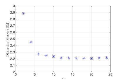
Figure 7: Experimental results from the experiment we performed to pick the best value for $c$ in equation 16. The figure shows the overall distortion metric of equation 21 computed from the $24$ SLADS experiments for the $c=2,4,6,\ldots 24$. The distortion metric is smallest when $c=20$.

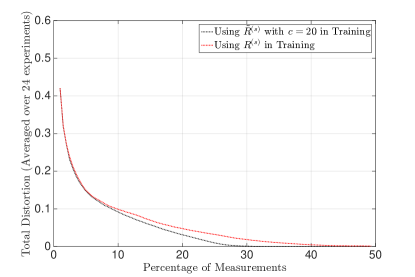
Figure 8: Experimental results from the experiments we performed to empirically validate the approximation to the $ERD$. The curves show the TD averaged over $24$ different experiments versus the percentage of samples when the true value of $R^{(s)}$ was used to estimate $\theta$ and when the approximate value of $R^{(s)}$ was used to estimate $\theta$. In this experiments we selected $c=20$ to compute the approximate RD.

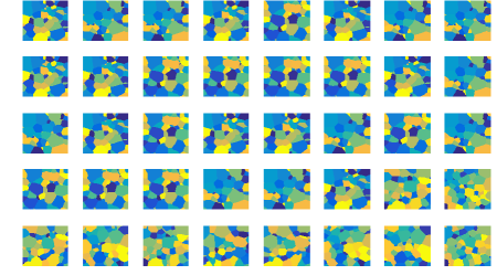
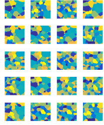
Figure 9: Images used for training and testing in the experiment detailed in Section VI-B in which we compared SLADS with LS and RS. These images have $512\times 512$ pixels each, and are synthetic EBSD image generated using the Dream.3D software. The images here are discretely labeled and the different colors correspond to different crystal orientations. In particular, (a): shows the images that were used for training and (b): shows the images that were used for testing.

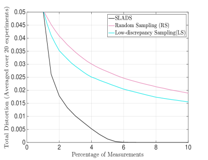
Figure 10: In this figure we plot the average $TD$, $\bar{TD}_{k}$, (averaged over $20$ sampling experiments) versus the percentage of samples for the experiment detailed in Section VI-B. The plot shows the $\bar{TD}_{k}$ curves that correspond to SLADS, RS and LS. The images that were sampled in this experiment are shown in Figure 9(b).

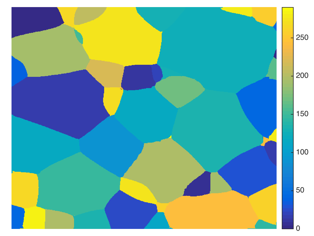
(a) Original Image

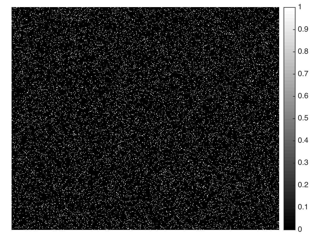
(b) RS: Sample locations ($\sim 6\%$)

(c) LS: Sample locations ($\sim 6\%$)

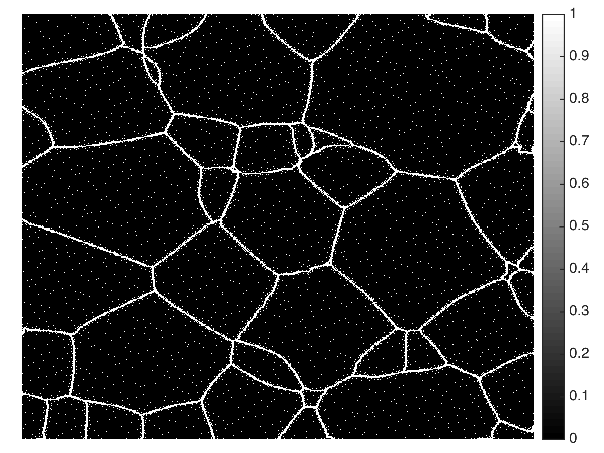
(d) SLADS: Sample locations ($\sim 6\%$)

(e) RS: Reconstructed Image

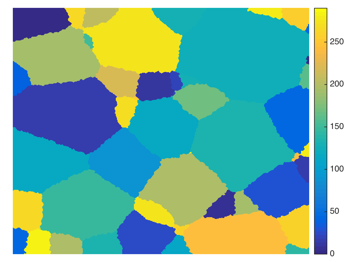
(f) LS: Reconstructed Image

(g) SLADS: Reconstructed Image

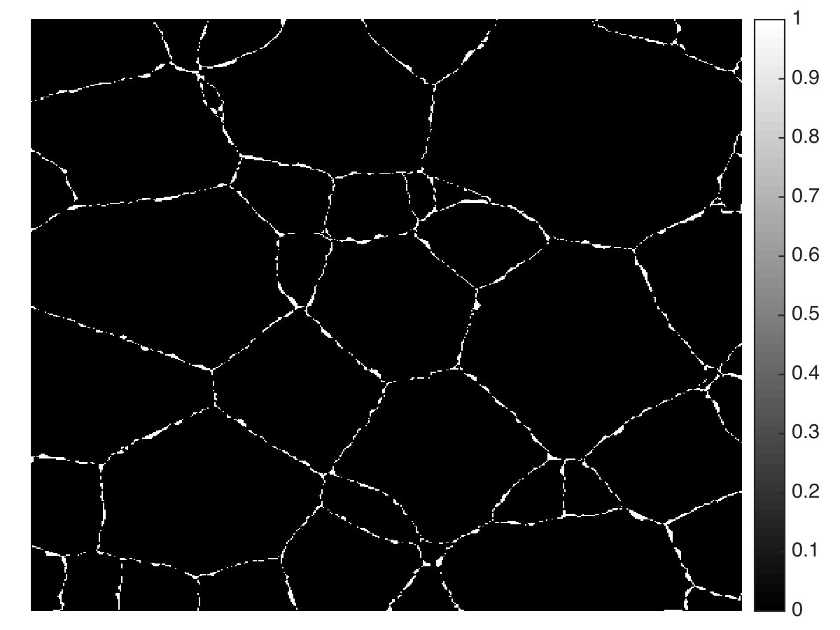
(h) RS: Distortion Image         (TD $=2.11\times 10^{-2}$)

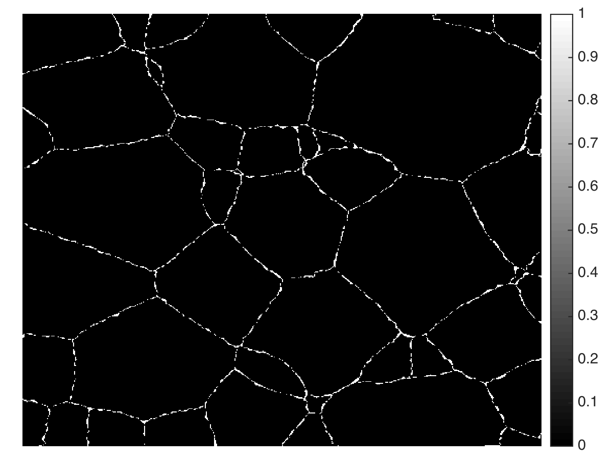
(i) LS: Distortion Image         (TD $=1.74\times 10^{-2}$)

(j) SLADS: Distortion Image         (TD $=3.81\times 10^{-6}$)

Figure 11: This figure shows sample locations and reconstructions after $6\%$ of the image in (a) was sampled using SLADS, RS and LS. Here (a) is the image being sampled. (b), (c) and (d) show the images reconstructed from samples collected using RS, LS and SLADS respectively. (e), (f) and (g) are the distortion images that correspond to (b), (c) and (d) respectively. A distortion image is defined as $D\left(X,\hat{X}\right)$ where $X$ is the ground truth and the $\hat{X}$ is the reconstructed image. Note that the distortion image only has values $0$ and $1$ since these are discretely labeled images (see Appendix -A). (h), (i) and (j) are the measurement masks that correspond to (b), (c) and (d) respectively.

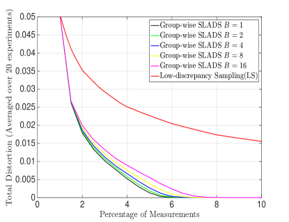
Figure 12: In this figure we compare SLADS with Group-wise SLADS. In particular, we performed SLADS and Group-wise SLADS with $B=2,4,8,16$ on $20$ simulated EBSD images shown in Figure 9(b) and then plotted $TD_{k}$ versus the percentage of samples. We see that Group-wise SLADS is comparable to SLADS and that as $B$ gets larger the distortion for the same number of samples gets larger. Note that SLADS is group-wise SLADS with $B=1$.

VI-B Results using Simulated EBSD Images

In this section we first compare SLADS with two static sampling methods – Random Sampling (RS) [5] and Low-discrepancy Sampling (LS) [6]. Then we evaluate the group-wise SLADS method introduced in Section V and finally we evaluate the stopping method introduced in Section IV. Figures 9(a) and 9(b) show the simulated $512\times 512$ EBSD images we used for training and testing, respectively, for all the experiments in this section. All results used the parameter value $c^{*}=10$ that was estimated using the method described in Section III-C. The average total distortion, $\overline{TD}_{k}$, for the experiments was computed over the full test set of images.

Figure 10 shows a plot of the average total distortion, $\overline{TD}_{k}$, for each of the three algorithms that were compared, LS, RS and SLADS. Notice that SLADS dramatically reduces error relative to LS or RS at the same percentage of samples, and that it achieves nearly perfect reconstruction after approximately $6\%$ of the samples are measured.

Figure 11 gives some insight into the methods by showing the sampled pixel locations after $6\%$ of samples have been taken for each of the three methods. Notice that SLADS primarily samples in locations along edges, but also selects some points in uniform regions. This both localizes the edges more precisely while also reducing the possibility of missing a small region or “island” in the center of a uniform region. Alternatively, the LS and RS algorithms select sample locations independent of the measurements; so samples are used less efficiently, and the resulting reconstructions have substantially more errors along boundaries.

To evaluate the group-wise SLADS method we compare it with SLADS and LS. Figure 12 shows a plot of the average total distortion, $\overline{TD}_{k}$, for SLADS, LS, group-wise SLADS with the group sampling rates of $B=2,4,8$ and $16$ performed on the images in Figure 9(b). We see that group-wise SLADS has somewhat higher distortion for the same number of samples as SLADS and that the distortion increases with increasing values of $B$. This is reasonable since SLADS without group sampling has the advantage of having the most information available when choosing each new sample. However, even when collecting $B=16$ samples in a group, the increase in distortion is still dramatically reduced relative to LS sampling.

We then evaluate the stopping method by attempting to stop SLADS at different distortion levels. In particular, we will attempt to stop SLADS when $TD_{k}\leq TD_{desired}$ for $TD_{desired}=\left\{5\times 10^{-5},10\times 10^{-5},15\times 10^{-5}\ldots 50\times 10^{-5}\right\}$. For each $TD_{desired}$ value we found the threshold to place on the stopping function, in equation 23, by using the method described in Section IV on a subset of the images in Figure 9(a). Again we used the images shown in Figures 9(a) and 9(b) for training and testing, respectively. After each SLADS experiment stopped we computed the true $TD$ value, ${TD}_{true}$, and then computed the average true $TD$ value for a given $TD_{desired}$, $\bar{TD}_{true}\left(TD_{desired}\right)$, by averaging the ${TD}_{true}$ values over the $20$ testing images.

Figure 13 shows a plot of $\bar{TD}_{true}\left(TD_{desired}\right)$ and $TD_{desired}$. From this plot we can see that the experiments that in general $TD_{desired}\geq\bar{TD}_{true}\left(TD_{desired}\right)$. This is the desirable result since we intended to stop when $TD_{k}\leq TD_{desired}$. However, from the standard deviation bars we see that in certain experiments the deviation from $TD_{desired}$ is somewhat high and therefore note the need for improvement through future research.

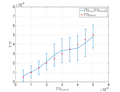
Figure 13: This plot corresponds to the experiment performed to evaluate the stopping method we presented in Section IV. Here we plot $\bar{TD}_{true}\left(TD_{desired}\right)$ and $TD_{desired}$ where $TD_{desired}=\left\{5\times 10^{-5},10\times 10^{-5},15\times 10^{-5}\ldots 50\times 10^{-5}\right\}$. $\bar{TD}_{true}\left(TD_{desired}\right)$ was computed by averaging the ${TD}_{true}$ values over $10$ experiments. Note that we also show the standard deviation bars for $\bar{TD}_{true}\left(TD_{desired}\right)$. From this plot we see that the stopping method on average is accurate.

It is also important to mention that the SLADS algorithm (for discrete images) was implemented for protein crystal positioning by Simpson et al. in the synchrotron facility at the Argonne national laboratory [1].

VI-C Results using Scanning Electron Microscope Images

(a) Original Image

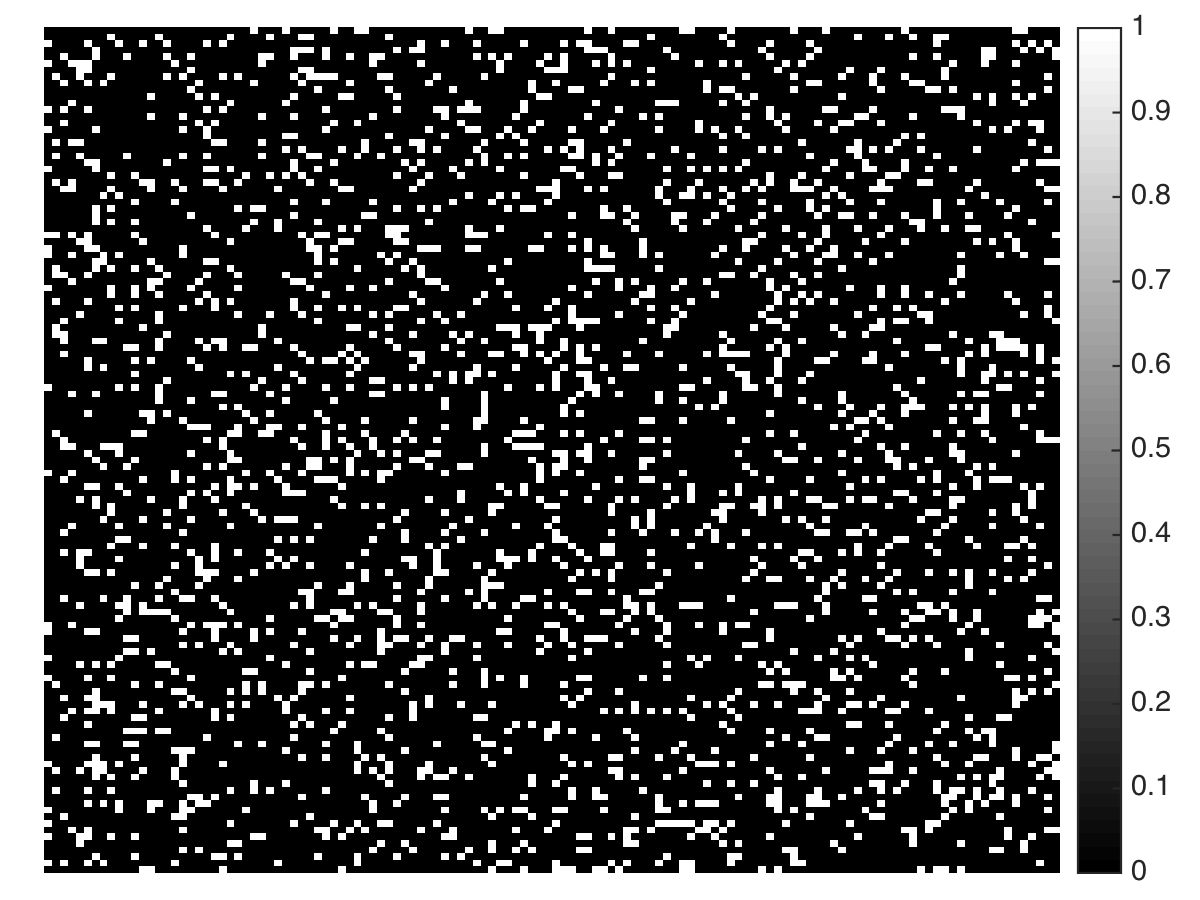
(b) RS: Sample locations         ($\sim 15\%$)

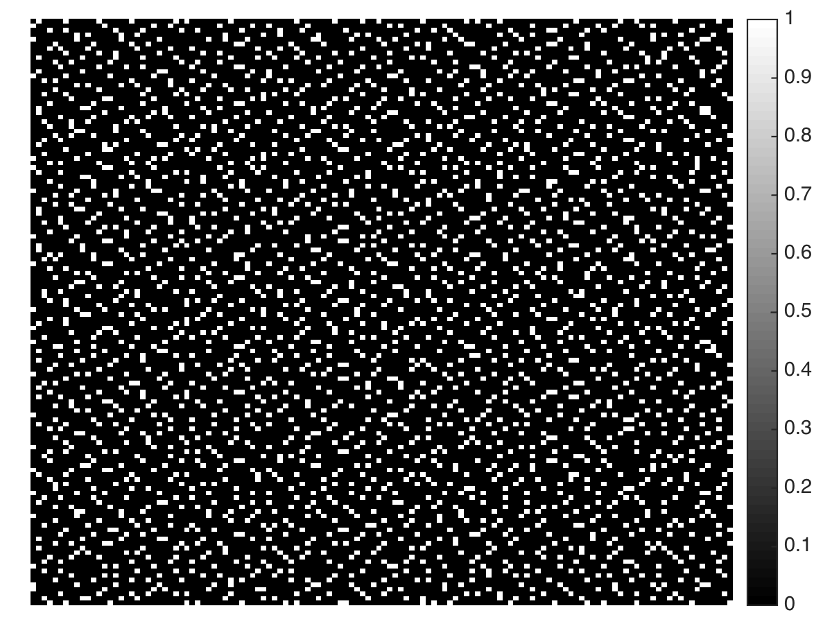
(c) LS: Sample locations         ($\sim 15\%$)

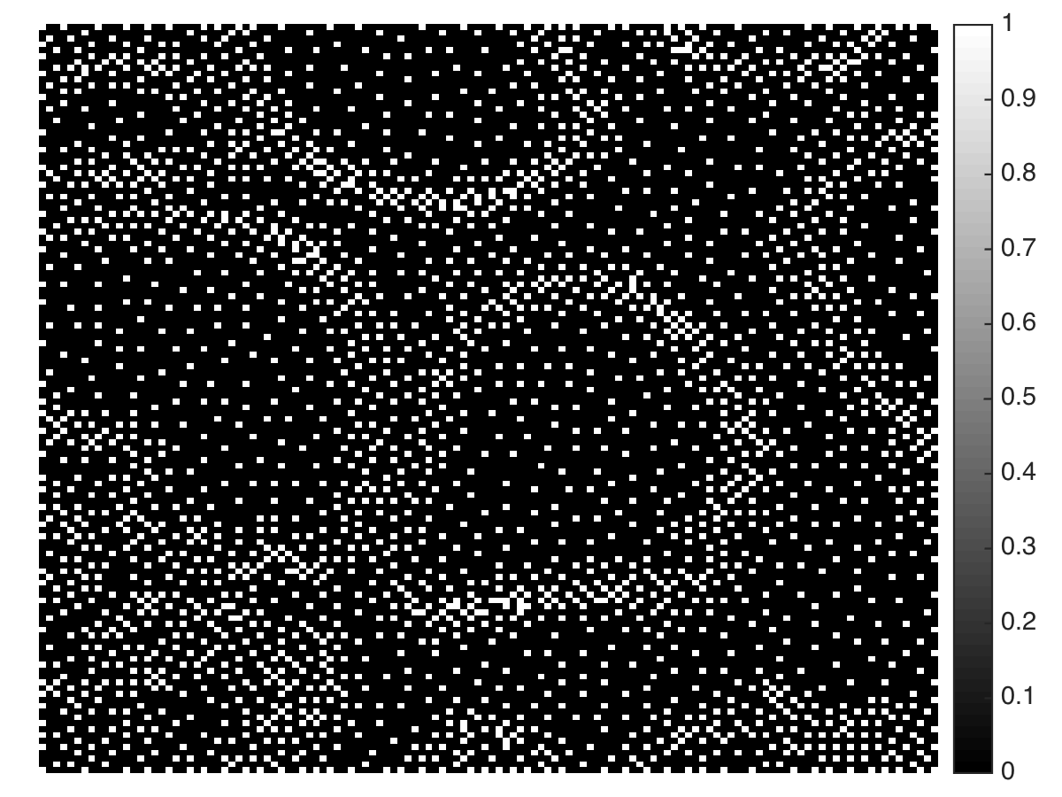
(d) SLADS: Sample locations ($\sim 15\%$)

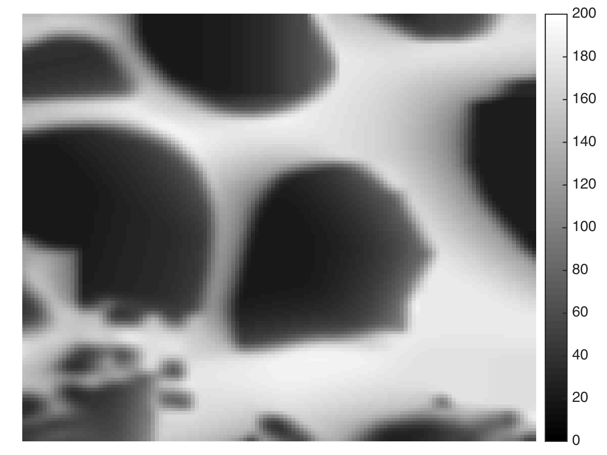
(e) RS: Reconstructed Image

(f) LS: Reconstructed Image

(g) SLADS: Reconstructed Image

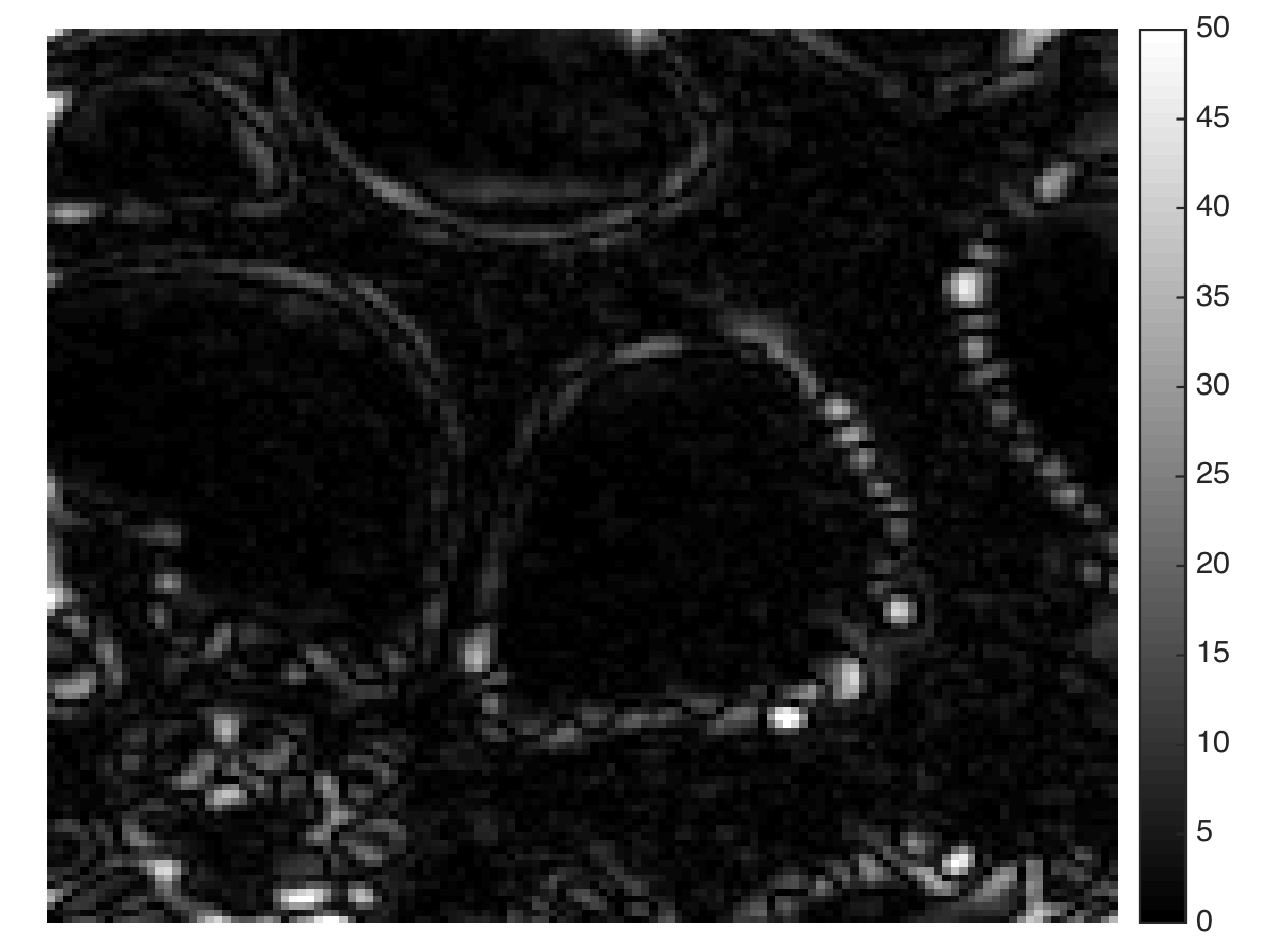
(h) RS: Distortion Image         (TD $=3.88$)

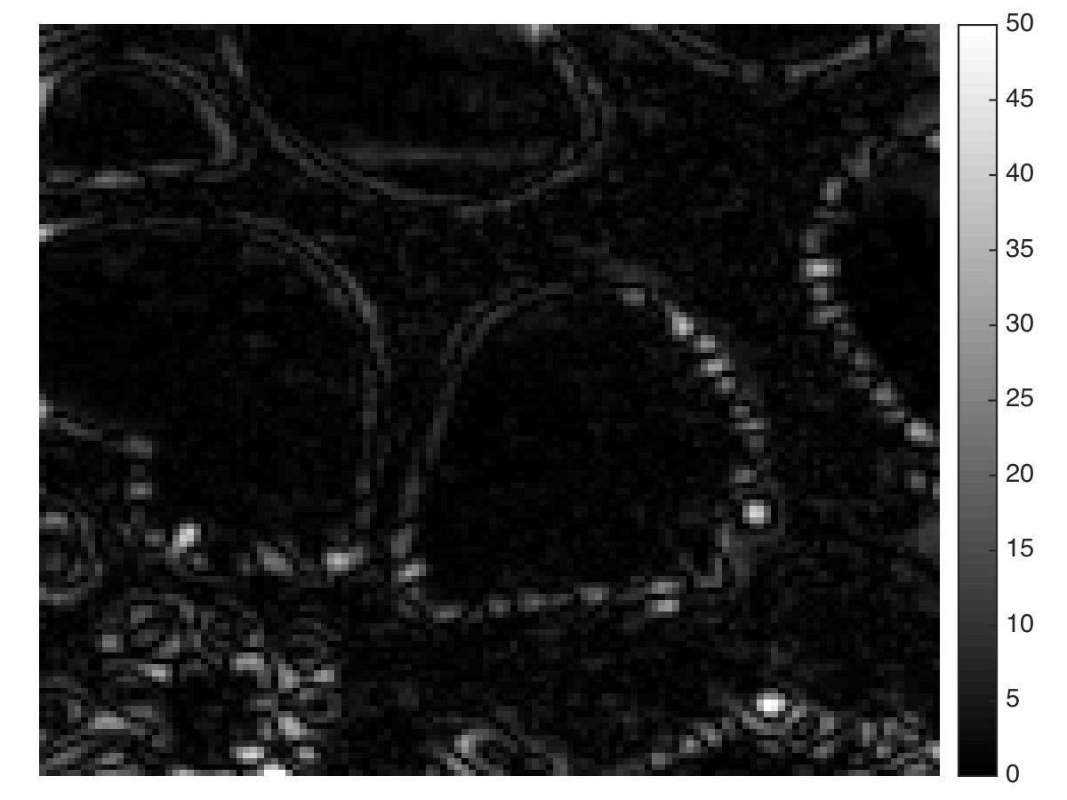
(i) LS: Distortion Image         (TD $=3.44$)

(j) SLADS: Distortion Image         (TD $=2.63$)

Figure 14: This figure shows sample locations and reconstructions after $15\%$ of the image in (a) was sampled using SLADS, RS and LS. Here (a) is the image being sampled. (b), (c) and (d) show the images reconstructed from samples collected using RS, LS and SLADS respectively. (e), (f) and (g) are the distortion images that correspond to (b), (c) and (d) respectively. A distortion image is defined as $D\left(X,\hat{X}\right)$ where $X$ is the ground truth and the $\hat{X}$ is the reconstructed image. Note that the distortion image has values ranging from $0$ to $255$ since these are continuous $8$ bit images (see Appendix -A). (h), (i) and (j) are the measurement masks that correspond to (b), (c) and (d) respectively.

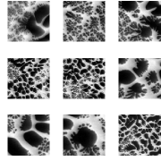
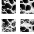
Figure 15: Images used for training and testing in the experiment detailed in Section VI-C in which we compared SLADS with LS and RS. These images have $128\times 128$ pixels each, and experimental collected SEM images. In particular, (a) shows the images that were used for training and (b) shows the images that were used for testing. These images were collected by Ali Khosravani & Prof. Surya Kalidindi from Georgia Institute of Technology.

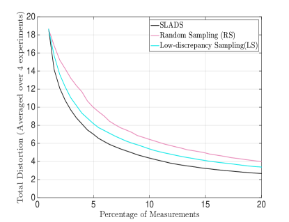
Figure 16: In this figure we plot the average $TD$,$\bar{TD}_{k}$, (averaged over $4$ sampling experiments) versus the percentage of samples for the experiment detailed in Section VI-C. The plot shows the $\bar{TD}_{k}$ curves that correspond to SLADS, RS and LS. The images that were sampled in this experiment are shown in Figure 15(b).

In this section we again compare SLADS with LS and RS but now on continuously valued scanning electron microscope (SEM) images. Figures 15(a) and 15(b) show the $128\times 128$ SEM images used for training and testing, respectively. Using the methods described in Section III-C, the parameter value $c^{*}=2$ was estimated and again the average total distortion, $\overline{TD}_{k}$ was computed over the full test set of images.

Figure 16 shows a plot of $\overline{TD}_{k}$ for each of the three tested algorithms, SLADS, RS, and LS. We again see that SLADS outperforms the static sampling methods, but not as dramatically as in the discrete case.

Figure 14 shows the results of the three sampling methods after $15\%$ of the samples have been taken along with the resulting sampling locations that were measured. Once more we notice that SLADS primarily samples along edges, and therefore we get better edge resolution. We also notice that some of the smaller dark regions (“islands”) are missed by LS and RS while SLADS is able to resolve almost all of them.

VII Conclusions

In this paper, we presented a framework for dynamic image sampling which we call a supervised learning approach to dynamic sampling (SLADS). The method works by selecting the next measurement location in a manner that minimizes the expected reduction in distortion (ERD) for each new measurement. The SLADS algorithm dramatically reduces the computation required for dynamic sampling by using a supervised learning approach in which a regression algorithm is used to efficiently estimate the ERD for each new measurement. This makes the SLADS algorithm practical for real-time implementation.

Our experiments show that SLADS can dramatically outperform static sampling methods for the measurement of discrete data. For example, SEM analytical methods such as EBSD[2], or synchrotron crystal imaging [1] are just two cases in which sampling of discrete images is important. We also introduced a group-wise SLADS method which allows for sampling of multiple pixels in a group, with only limited loss in performance. Finally, we concluded with simulations on sampling from continuous SEM images in which we demonstrated that SLADS provides modest improvements compared to static sampling.

-A Distortion Metrics for Experiments

Applications such as EBSD generate images formed by discrete classes. For these images, we use a distortion metric defined between two vectors $A\in\mathbb{R}^{N}$ and $B\in\mathbb{R}^{N}$ as

$$D\left(A,B\right)=\displaystyle\sum\limits_{i=1}^{N}I\left(A_{i},B_{i}\right),$$ (31)

where $I$ is an indicator function defined as

$$I\left(A_{i},B_{i}\right)=\begin{cases}0\quad A_{i}=B_{i}\\ 1\quad A_{i}\neq B_{i},\end{cases}$$ (32)

where $A_{i}$ is the $i^{th}$ element of the vector $i$.

However, for the experiments in Section VI-C we used continuously valued images. Therefore, we defined the distortion $D\left(A,B\right)$ between two vectors $A$ and $B$ as

$$D\left(A,B\right)=\displaystyle\sum\limits_{i=1}^{N}|A_{i}-B_{i}|.$$ (33)

-B Reconstruction Methods for Experiments

In the experiments with discrete images experiments all the reconstructions were performed using the weighted mode interpolation method. The weighted mode interpolation of a pixel $s$ is $X_{\hat{r}}$ for

$$\hat{r}=\arg\max_{r\in\partial s}\left\{\displaystyle\sum\limits_{t\in\partial s}\left[\left(1-D\left(X_{r},X_{t}\right)\right)w_{r}^{(s)}\right]\right\},$$ (34)

where

$$w_{r}^{(s)}=\frac{\frac{1}{\|s-r\|^{2}}}{\displaystyle\sum\limits_{u\in\partial s}\frac{1}{\|s-u\|^{2}}}$$ (35)

and $|\partial s|=10$.

In the training phase of the experiments on continuously valued data, we performed reconstructions using the Plug & Play algorithm [21] to compute the reduction-in-distortion. However, to compute the reconstructions for descriptors (both in testing and training) we used weighted mean interpolation instead of Plug & Play to minimize the run-time speed of SLADS. We define the weighted mean for a location $s$ by

$$\hat{X}_{s}=\displaystyle\sum\limits_{r\in\partial s}w_{r}^{(s)}X_{r}.$$ (36)

References

- [1] N. M. Scarborough, G. M. D. P. Godaliyadda, D. H. Ye, D. J. Kissick, S. Zhang, J. A. Newman, M. J. Sheedlo, A. U. Chowdhury, R. F. Fischetti, C. Das, G. T. Buzzard, C. A. Bouman, and G. J. Simpson, “Dynamic x-ray diffraction sampling for protein crystal positioning,” Journal of Synchrotron Radiation, vol. 24, no. 1, pp. 188–195, January 2017.
- [2] A. J. Schwartz, M. Kumar, B. L., and D. P. A. Field, Electron Backscatter Diffraction in Materials Science. Springer US, 2009.
- [3] R. Smith-Bindman, J. Lipson, and R. Marcus, “Radiation dose associated with common computed tomography examinations and the associated lifetime attributable risk of cancer,” Archives of Internal Medicine, vol. 169, no. 22, pp. 2078–2086, 2009.
- [4] R. F. Egerton, P. Li, and M. Malac, “Radiation damage in the tem and sem,” Micron, vol. 35, no. 6, pp. 399 – 409, 2004, international Wuhan Symposium on Advanced Electron Microscopy. [Online]. Available: http://www.sciencedirect.com/science/article/pii/S0968432804000381
- [5] H. S. Anderson, J. Ilic-Helms, B. Rohrer, J. Wheeler, and K. Larson, “Sparse imaging for fast electron microscopy,” IS&T/SPIE Electronic Imaging, pp. 86 570C–86 570C, 2013.
- [6] R. Ohbuchi and M. Aono, “Quasi-monte carlo rendering with adaptive sampling,” 1996.
- [7] K. A. Mohan, S. V. Venkatakrishnan, J. W. Gibbs, E. B. Gulsoy, X. Xiao, M. D. Graef, P. W. Voorhees, and C. A. Bouman, “Timbir: A method for time-space reconstruction from interlaced views,” IEEE Transactions on Computational Imaging, pp. 96–111, June 2015.
- [8] K. Mueller, “Selection of optimal views for computed tomography reconstruction,” Patent WO 2,011,011,684, Jan. 28, 2011.
- [9] Z. Wang and G. R. Arce, “Variable density compressed image sampling,” Image Processing, IEEE Transactions on, vol. 19, no. 1, pp. 264–270, 2010.
- [10] M. W. Seeger and H. Nickisch, “Compressed sensing and bayesian experimental design,” in Proceedings of the 25th international conference on Machine learning. ACM, 2008, pp. 912–919.
- [11] W. R. Carson, M. Chen, M. R. D. Rodrigues, R. Calderbank, and L. Carin, “Communications-inspired projection design with application to compressive sensing,” SIAM Journal on Imaging Sciences, vol. 5, no. 4, pp. 1185–1212, 2012.
- [12] S. Ji, Y. Xue, and L. Carin, “Bayesian compressive sensing,” IEEE Trans. on Signal Processing, vol. 56, no. 6, pp. 2346–2356, 2008.
- [13] J. Vanlier, C. A. Tiemann, P. A. J. Hilbers, and N. A. W. van Riel, “A bayesian approach to targeted experiment design,” Bioinformatics, vol. 28, no. 8, pp. 1136–1142, 2012.
- [14] A. C. Atkinson, A. N. Donev, and R. D. Tobias, Optimum experimental designs, with SAS. Oxford University Press, Oxford, 2007, vol. 34.
- [15] M. Seeger, H. Nickisch, R. Pohmann, and B. Schölkopf, “Optimization of k-space trajectories for compressed sensing by bayesian experimental design,” Magnetic Resonance in Medicine, vol. 63, no. 1, pp. 116–126, 2010.
- [16] K. Joost Batenburg, W. J. Palenstijn, P. Balázs, and J. Sijbers, “Dynamic angle selection in binary tomography,” Computer Vision and Image Understanding, 2012.
- [17] T. E. Merryman and J. Kovacevic, “An adaptive multirate algorithm for acquisition of fluorescence microscopy data sets,” IEEE Trans. on Image Processing, vol. 14, no. 9, pp. 1246–1253, 2005.
- [18] G. M. D. Godaliyadda, G. T. Buzzard, and C. A. Bouman, “A model-based framework for fast dynamic image sampling,” in proceedings of IEEE International Conference on Acoustics Speech and Signal Processing, 2014, pp. 1822–6.
- [19] G. D. Godaliyadda, D. Hye Ye, M. A. Uchic, M. A. Groeber, G. T. Buzzard, and C. A. Bouman, “A supervised learning approach for dynamic sampling,” in IS&T Imaging. International Society for Optics and Photonics, 2016.
- [20] M. A. Groeber and M. A. Jackson, “Dream. 3d: a digital representation environment for the analysis of microstructure in 3d,” Integrating Materials and Manufacturing Innovation 3.1, vol. 19, pp. 1–17, 2014.
- [21] S. Sreehari, S. V. Venkatakrishnan, L. F. Drummy, J. P. Simmons, and C. A. Bouman, “Advanced prior modeling for 3d bright field electron tomography,” in IS&T/SPIE Electronic Imaging. International Society for Optics and Photonics, 2015, pp. 940 108–940 108.
- [22] J. Haupt, R. Baraniuk, R. Castro, and R. Nowak, “Sequentially designed compressed sensing,” in Statistical Signal Processing Workshop (SSP). IEEE, 2012, pp. 401–404.
- [23] C. Jackson, R. F. Murphy, and J. Kovacevic, “Intelligent acquisition and learning of fluorescence microscope data models,” IEEE Trans. on Image Processing, vol. 18, no. 9, pp. 2071–2084, 2009.
- [24] X. Huan and Y. M. Marzouk, “Simulation-based optimal bayesian experimental design for nonlinear systems,” Journal of Computational Physic 232.1, pp. 288–317, 2013.