The mother of all states of the kagome quantum antiferromagnet

Frustrated quantum magnets are a central theme in condensed matter physics due to the richness of their phase diagrams. They support a panoply of phases including various ordered states and topological phases. Yet, this problem has defied solution for a long time due to the lack of controlled approximations which make it difficult to distinguish between competing phases. Here we report the discovery of a special quantum macroscopically degenerate point in the $XXZ$ model on the spin 1/2 kagome quantum antiferromagnet for the ratio of Ising to antiferromagnetic transverse coupling $J_{z}/J=-1/2$. This point is proximate to many competing phases explaining the source of the complexity of the phase diagram. We identify five phases near this point including both spin-liquid and broken-symmetry phases and give evidence that the kagome Heisenberg antiferromagnet is close to a transition between two phases.

The history of quantum frustrated magnetism began in 1973 with Anderson’s suggestion that the ground state of the nearest-neighbor (n.n.) Heisenberg model on the triangular lattice was a quantum spin-liquid Anderson (1973). While we now know that this particular model does not support a spin-liquid, both experimental and theoretical evidence has been building for quantum spin-liquids in various lattices built of triangular motifs. Materials such as Herbertsmithite (a kagome lattice of Cu²⁺ ions) Helton et al. (2007) and $\textrm{Na}_{4}\textrm{Ir}_{3}\textrm{O}_{8}$ (a hyper-kagome lattice of Ir⁴⁺ ions) Okamoto et al. (2007) fail to order down to low temperatures suggesting a possible spin-liquid ground state. This is supported by theoretical calculations which show that a panoply of spin-liquids (or exotic ordered phases) occur in a variety of Hamiltonians Zeng and Elser (1990); Singh and Huse (2007); Ran et al. (2007); Yan et al. (2011); Depenbrock et al. (2012); Iqbal et al. (2013); Jiang et al. (2012); Clark et al. (2013); Tay and Motrunich (2011); He et al. (2017); Liao et al. (2017); He and Chen (2015); Changlani and Läuchli (2015); Yao et al. (2015). This Letter presents an explanation of multiple energetically competitive phases in these models.

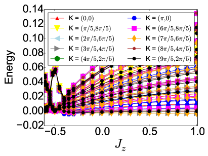
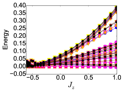
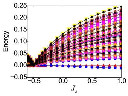
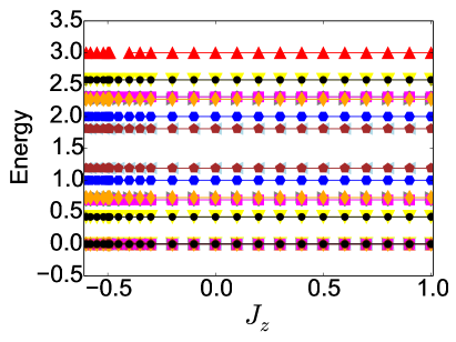
Figure 1: (Color online) Energy spectra (showing the 8 lowest energies in every momentum sector with respect to the lowest energy state in $K=(0,0)$) versus $J_{z}$ for a 30 site kagome cluster with periodic boundary conditions. The panels correspond to various $S_{z}$ sectors, (top left) $S_{z}=0$, (top right) $S_{z}=5$, (bottom left) $S_{z}=10$, (bottom right) $S_{z}=14$. A quantum degeneracy is seen at $J_{z}=-1/2$. The case of $S_{z}=14$ corresponds to one spin down in a sea of up spins and maps to the non-interacting solution, hence the spectrum does not change with $J_{z}.$

We first report the existence of a new macroscopic quantum degenerate point on kagome and hyper-kagome lattices in the spin-1/2 $XXZ$ Hamiltonian Yamamoto et al. (2014); Sellmann et al. (2015); Chernyshev and Zhitomirsky (2014); Götze and Richter (2015); Kumar et al. (2014, 2016),

$$H_{XXZ}[J_{z}]=\sum_{\langle i,j\rangle}S^{x}_{i}S^{x}_{j}+S^{y}_{i}S^{y}_{j}+J_{z}\sum_{\langle i,j\rangle}S^{z}_{i}S^{z}_{j}$$ (1)

at $H_{\textrm{XXZ}}[-1/2]$ (notated as $H_{XXZ0}$ Essafi et al. (2016)). $S_{i}$ are spin-1/2 operators on site $i$, $\langle i,j\rangle$ refer to nearest neighbor pairs and $J_{z}$ is the Ising coupling. The degeneracy exists in all $S_{z}$ sectors and all finite system sizes. For kagome, we explicitly demonstrate this in Fig. 1 where we perform an exact diagonalization (ED) on the $N=30$ site kagome cluster in different $S_{z}$ sectors. As we approach $J_{z}=-1/2$ many eigenstates collapse to the same ground state eigenvalue.

We solve analytically for much of the exponential manifold, and our solutions apply to any lattice of triangular motifs with the Hamiltonian of the form,

$$H=\sum_{\Delta}H_{XXZ0}(\Delta)$$ (2)

where $H_{XXZ0}(\Delta)$ is the $XXZ0$ Hamiltonian on a triangle $\Delta$, as long as its vertices can be colored by three colors with no two connected vertices being assigned the same color. Some three-colorable lattices with representative three-colorings are shown in Fig. 2. Our general result overlaps the $XXZ0$ point on the triangular lattice of Ref. Momoi and Suzuki (1992) and a different analytically solvable Hamiltonian on the zig-zag ladder of Ref. Batista (2009).

Finally, we show how the $XXZ0$ point on the kagome lattice is embedded in the wider phase diagram demonstrating its relation to the previously discovered spin-liquid at the Heisenberg point Yan et al. (2011); Depenbrock et al. (2012); Jiang et al. (2012) as well as nearby magnetically ordered phases; our results suggest an additional intermediate phase transition in the middle of the spin-liquid region.

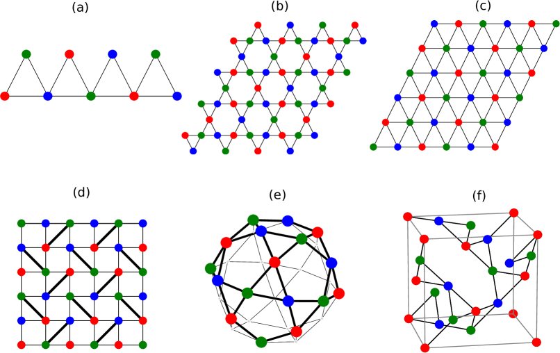
Figure 2: (Color online): Representative three-coloring solutions on various lattices with triangular motifs. (a) Saw-tooth (b) Kagome (c) Triangular (d) Shastry-Sutherland Shastry and Sutherland (1981) (with $J_{2}=2J_{1}$, note, the bold diagonal lines are associated with two triangles whereas other edges are part of only one triangle) (e) Icosidodecahedron (f) Hyper-kagome lattice

Exact Ground States at $J_{z}=-1/2$ — Any Hamiltonian of the form of Eq. (2) has ground states of the form

$$|C\rangle\equiv P_{S_{z}}\Big{(}\prod_{\text{valid}}\otimes|\gamma_{s}\rangle\Big{)}$$ (3)

where $\{|\gamma_{s}\rangle=|a\rangle,|b\rangle\text{ or }|c\rangle\}$, denoted as "colors" on site $s$ are defined as, $|a\rangle\equiv\frac{1}{\sqrt{2}}\Big{(}|\uparrow\rangle+|\downarrow\rangle\Big{)}$, $|b\rangle\equiv\frac{1}{\sqrt{2}}\Big{(}|\uparrow\rangle+\omega|\downarrow\rangle\Big{)}$, $|c\rangle\equiv\frac{1}{\sqrt{2}}\Big{(}|\uparrow\rangle+\omega^{2}|\downarrow\rangle\Big{)}$, where $\omega=e^{i2\pi/3}$. Taking the quantization axis to be the $z$-axis, the colors correspond to spin directions in the $XY$ plane that are at $120$ degrees relative to one another. Valid colorings satisfy the three-coloring condition. $P_{S_{z}}$ projects into a particular total $S_{z}$ sector.

For $J_{z}=-1/2$ and a single triangle, six states; the fully polarized state $|\uparrow\uparrow\uparrow\rangle$ and the chiral states $|\uparrow\downarrow\downarrow\rangle+\omega|\downarrow\uparrow\downarrow\rangle+{\omega}^{2}|\downarrow\downarrow\uparrow\rangle$ and $|\uparrow\downarrow\downarrow\rangle+{\omega}^{2}|\downarrow\uparrow\downarrow\rangle+{\omega}|\downarrow\downarrow\uparrow\rangle$ and all their Kramers pairs; are exactly degenerate. Thus Eq. (2) is recast as,

$$H=\sum_{\Delta}H_{\Delta}=\frac{3}{2}\sum_{\Delta}P_{\Delta}-\frac{3}{8}N_{\Delta}$$ (4)

where $N_{\Delta}$ is the number of triangles and $P_{\Delta}$ is a projector on the triangle $P_{\Delta}\equiv|+\rangle\langle+|+|-\rangle\langle-|$ and $|+\rangle$ and $|-\rangle$ are Kramers pairs of non-chiral one-magnon states on the triangle, $|+\rangle\equiv\frac{1}{\sqrt{3}}\Big{(}|\uparrow\uparrow\downarrow\rangle+|\uparrow\downarrow\uparrow\rangle+|\downarrow\uparrow\uparrow\rangle\Big{)}$ and $|-\rangle\equiv\frac{1}{\sqrt{3}}\Big{(}|\downarrow\downarrow\uparrow\rangle+|\downarrow\uparrow\downarrow\rangle+|\uparrow\downarrow\downarrow\rangle\Big{)}$ This rewriting can be carried out on any lattice of triangles; if a bond is used by multiple triangles this constrains the coupling constant between these bonds.

The $XXZ0$ Hamiltonian is thus a sum of positive semi-definite non-commuting projectors. Any wavefunction that simultaneously zeroes out each projector consistently is guaranteed to be a ground state. Such "frustration-free" Hamiltonians include Majumdar-Ghosh Majumdar and Ghosh (1969) (generalized by Klein Klein (1982)) and Affleck-Kennedy-Lieb-Tasaki Affleck et al. (1987); Wen (2003); Kitaev (2003); Wang et al. (2017) Hamiltonians. Zeroing out a projector requires that only components exactly orthogonal to states $|+\rangle$ and $|-\rangle$ enter the full many body wavefunction; this is indeed achieved by the product state $|\psi\rangle\equiv\prod_{\textrm{valid}}\otimes|\gamma_{s}\rangle$. We also note that such "three-coloring states" have a long history and have been explored in several contexts Harris et al. (1992); Henley (2009); Huse and Rutenberg (1992); Chalker et al. (1992); Sachdev (1992); Cépas and Ralko (2011); Essafi et al. (2016); Castelnovo et al. (2005).

The product state $|\psi\rangle$ does not conserve total $S_{z}$ but the $XXZ$ Hamiltonian does conserve it. Therefore, projecting each three-coloring solution to each $S_{z}$ sector is also a ground state leading to Eq. (3). Note that three-colorings which differ simply by relabeling colors are identical up to a global phase (see Supplement).

Lattice	Method	$\;\;n_{b}=1\;\;$	$\;\;n_{b}=2\;\;$	$\;\;n_{b}=3\;\;$	$\;\;n_{b}=4\;\;$	$\;\;n_{b}=5\;\;$	$\;\;n_{b}=6\;\;$	$n_{b}=\lfloor N/2\rfloor$	# 3-colorings
sawtooth obc	ED	6	16	26	31	32	32	32	32
$5$ triangles	$R(S)$	6	16	26	31	32	32	32
$3\times 3$ kagome obc	ED	15	102	414	1117				3808
(33 sites)	$R(S)$	15	102	414	1117	2136	3078	3808
$3\times 3$ kagome pbc	ED	10	38	60	41	40	40	40	40
	$R(S)$	10	34	40	40	40	40	40
$4\times 3$ kagome pbc	ED	13	68	169	172	137	136		136
	$R(S)$	13	68	134	136	136	136	136

Table 1: Number of ground states in different $S_{z}$ sectors (mapped to hard-core boson number $n_{b}$) on several lattices (of size $N$) with triangular motifs at $J_{z}=-1/2$, $J_{2}=0$. $R(S)$ is the rank of the overlap matrix indicating the number of linearly independent 3-coloring modes and ED refers to the exact number of ground states. The kagome cluster with open boundary conditions (obc) has completed triangles, resembling the periodic counterpart (pbc) in appearance.

Macroscopic Degeneracy and additional ground states— While there are only two ways of three-coloring the triangular lattice, there are an exponential number of ways of doing so on the kagome (scaling as $1.208^{N}$ Baxter (1970)) and hyper-kagome lattices. The precise number of ground states varies from sector to sector because of the loss of linear independence of the unprojected solutions under projection. For typical $S_{z}$ of interest, particularly $S_{z}=0$, there are still an exponential number of linearly independent solutions. This counting is made precise by forming the overlap matrix $S_{C,C^{\prime}}\equiv\langle C|C^{\prime}\rangle$ and evaluating its rank $\equiv R(S)$ numerically; our results have been shown in Table 1 and the Supplement. The case of one down spin in a sea of up spins which maps to the non-interacting problem with a flat-band with a quadratic band touching Bergman et al. (2008) is also correctly captured.

On several representative clusters with open boundary conditions (but always with completed triangles), we never find solutions outside the coloring manifold which suggests (but does not prove) the possibility that coloring solutions describe all degeneracies on open lattices. However, for kagome on tori we find, for low fillings, degenerate solutions not spanned by colorings.

Connection to the wider Kagome phase diagram— We now show how the $XXZ0$ point is embedded in the larger kagome phase diagram. We focus on $S_{z}=0$ and the fully symmetric sector of $K=(0,0)$ sector (see Supplement), and study an extended Hamiltonian involving nearest neighbor (nn) and next-nearest neighbor (nnn) terms,

$$H[J_{z},J_{2}]=H^{\textrm{nn}}_{XXZ}[J_{z}]+J_{2}H^{\textrm{nnn}}_{XXZ}[J_{z}]$$ (5)

where $H^{\textrm{nnn}}_{XXZ}[J_{z}]=\Big{(}\sum_{\langle\langle i,j\rangle\rangle}S^{x}_{i}S^{x}_{j}+S^{y}_{i}S^{y}_{j}+J_{z}S^{z}_{i}S^{z}_{j}\Big{)}$; $\langle\langle i,j\rangle\rangle$ referring to nnn pairs. We use a combination of analytical arguments and ED on the 36d cluster Leung and Elser (1993); Läuchli et al. (2011) on a grid of points in the $(J_{z},J_{2})$ space. As Fig. 3 shows, we find five phases near $XXZ0$: a ferromagnetic phase, a $q=0$ phase, a $\sqrt{3}\times\sqrt{3}$ phase and (potentially) two spin-liquids. We give numerical evidence that all these phases, other than the ferromagnet, connect from near (or touching) XXZ0 to the Heisenberg point.

At $J_{z}=-1/2$ and $J_{2}>0$, (notated AF-line) all triangles in the Hamiltonian are of the $XXZ0$ form and remain consistently three-colorable. Three-coloring both nn and nnn triangles constrains the allowed colorings leaving only two colorings in the well known $q=0$ pattern. This phase survives for $J_{z}>-1/2$, at small $J_{2}$, and is primarily identified by peaks at the $M$ point (Fig. S2 of the Supplement) in the spin-structure factor $S(\vec{q})\equiv\frac{1}{N}\sum_{i,j}\langle S_{i}\cdot S_{j}\rangle e^{i\vec{q}\cdot(\vec{r_{i}}-\vec{r_{j}})}$ where $\vec{r}_{i}$ refers to the real space coordinates of the $i^{th}$ lattice site, $N$ is the total number of sites and $\langle S_{i}\cdot S_{j}\rangle$ is the spin-spin correlation function. On the other hand, it can be rigorously shown the minimum energy state upon perturbing the AF-line to $J_{z}<-1/2$ is the fully polarized ferromagnetic state.

At $J_{z}=-1/2$ and $J_{2}<0$, we find evidence for the $\sqrt{3}\times\sqrt{3}$ phase. While we can not solve for the exact ground state, the state which colors nnn triangles the same color (i.e. the $\sqrt{3}\times\sqrt{3}$ phase) minimizes the nnn energy within the three-coloring manifold. We numerically verify this phase by looking at $S(K)$, finding it survives for $J_{z}$ near and on both sides of $-1/2$.

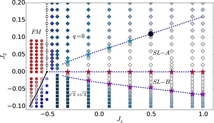
Figure 3: (Color online): The phase diagram in the $J_{z}-J_{2}$ plane on the 36d lattice showing five phases - the ferromagnet (FM), the magnetically ordered phases ($q=0$ and $\sqrt{3}\times\sqrt{3}$), and the spin liquids (SL-A and SL-B). Circles correspond to the energy difference $E(S_{z}=0)_{N=36}-E_{TDL}(S_{z}=N/2)$ between the $S_{z}=0$ sector and fully polarized state ranging from deep blue (negative) to deep red (positive). The diamonds are colored based on the structure factor at the $M$ point ($S(M)$) and squares are colored based on the structure factor at the $K$ point ($S(K)$). The darkest color corresponds to the largest structure factor on the graph. Star symbols correspond to location of fidelity dips and the error-bars indicate the uncertainty in the location of the phase boundaries (when scanned in the $J_{2}$ direction) and correspond to the grid-spacing used for the computation of the fidelity. The black hexagon (at $J_{z}\approx 0.5$, $J_{2}\approx 0.10$) is a kink in the second derivative of the fidelity; beyond the corresponding $J_{z}$ the fidelity dip is not noticeable and the phase boundary is just an extrapolation. Phase boundaries are marked with dotted lines, which are guides to the eye. The solid line is where the semiclassical energy difference between the FM and the unprojected $\sqrt{3}\times\sqrt{3}$ state goes to zero.

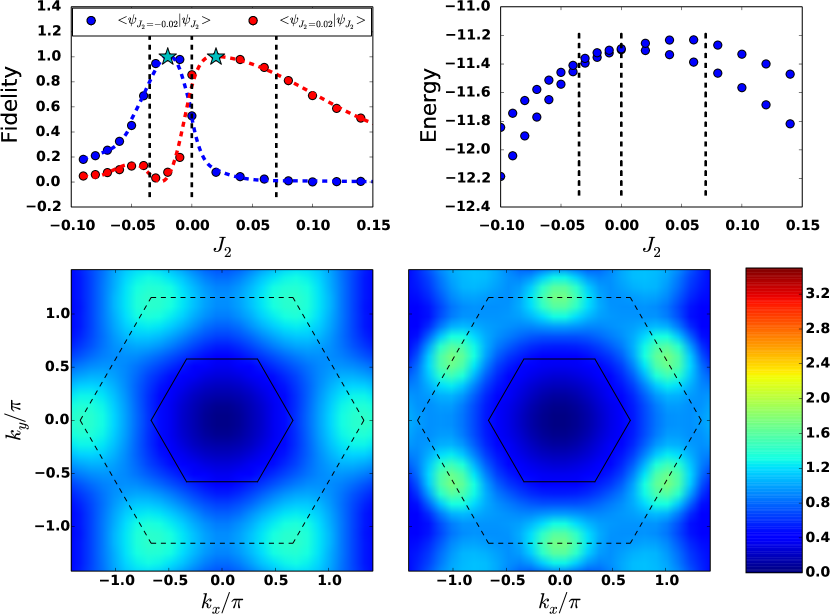
Figure 4: (Color online) All data is at $J_{z}=0.1$ for the 36d lattice. Top Left: Overlap of the ground state at $J_{2}$ with respect to reference ground state wavefunctions at $J_{2}=-0.02$ (blue) and $J_{2}=0.02$ (red). Dashed lines represent transitions as measured by fidelity. Top Right: Energy of the two lowest states in the symmetric representation of the $K=(0,0)$ sector. There are additional state(s) between these two states in other quantum-number sectors. Bottom: The static spin structure factor $S(\vec{q})$ of the ground state for $J_{2}=-0.02$ (left) and $J_{2}=0.02$ (right). The solid and the dotted lines show the first and the extended Brillouin zones respectively. The high symmetry points of the latter correspond to $K$ (corners of the hexagon) and $M$ (midpoints of edges) points. On going from $J_{2}<0$ to $J_{2}>0$, the intensity is transferred from $K$ to $M$ points.

By tracing paths through parameter space with large values of $S(\vec{q})$ at the $K$ and $M$ points, we find that both the $q=0$ phase and $\sqrt{3}\times\sqrt{3}$ phases near the $XXZ0$ point extend to the Heisenberg point at non-zero $J_{2}$. To locate the boundaries of these phases, we perform sweeps through $J_{2}$ at fixed $J_{z}$ and identify dips in the wavefunction fidelity defined to be

$$f(J_{z},J_{2})\equiv\Big{|}\langle\psi(J_{z},J_{2}-\Delta J_{2}/2)|\psi(J_{z},J_{2}+\Delta J_{2}/2)\rangle\Big{|}\\$$ (6)

where $\psi(J_{z},J_{2})$ is the ground state wavefunction, $\Delta J_{2}$ is the step size in the $J_{2}$ direction. For both magnetically ordered phases, the location of these dips form lines emanating from (or close to) the $XXZ0$ point that extrapolate to the Heisenberg point ($J_{z}=1$) to values $J_{2}\approx 0.16$ for $q=0$ and $J_{2}\approx-0.06$ for $\sqrt{3}\times\sqrt{3}$. These values are within the bounds previously found by a DMRG study Kolley et al. (2015), but disagree with a variational study by Ref. Iqbal et al. (2012) which finds instead a valence bond crystal. In the intermediate phase(s), we see a decrease in the magnitude of the structure factor peaks consistent with a change in phase to a spin-liquid.

Near $XXZ0$ we do not detect fidelity dips and see larger structure factors that extend much closer to the line $J_{2}=0.$ This leaves two plausible scenarios: (1) the spin-liquid(s) terminate at $J_{z}>-1/2$ for all $J_{2}$ or (2) the phase boundaries extend to $XXZ0$ but finite size-effects near it become large making it difficult to resolve the transition.

We find an additional fidelity dip at $J_{2}\approx 0$ and $J_{z}>-1/2$ in the region where other studies Kolley et al. (2015) identify a single spin-liquid phase. This interesting finding indicates the existence of an additional transition in this region. Our analysis in this work is largely ambivalent about the nature of these two phases but earlier evidence for a spin-liquid phase at $J_{z}=1$ and both $J_{2}>0,J_{2}<0$ Kolley et al. (2015); Liao et al. (2017) suggests a possible transition between two spin-liquids. Interestingly, a recent IPEPS study Jiang et al. (2016) found nearly degenerate variational degenerate energies for the $Q_{1}=Q_{2}$ and $Q_{1}=-Q_{2}$ Sachdev (1992) Z₂-spin liquids which they interpret as evidence for a parent U(1) DSL; given our results, another reasonable interpretation is that there is a transition between these two states.

To further understand the nature of the fidelity dips, we consider the ground state and excited state in the same quantum number sector as a function of $J_{2}$ at $J_{z}=0.1$ (Fig. 4, top right); the true first excited-state is in another sector. We see a (formally avoided) "level-crossing" indicated by a shrinking gap between these states around $J_{2}\approx 0$. This crossing causes the fidelity dip and leads to the overlap of the wavefunction on both sides of $J_{2}\approx 0$ being small with respect to a reference point on the other side (see Fig. 4, top left). In addition, the structure factors of the two ground states at positive and negative $J_{2}$, despite not having large peaks, are qualitatively distinct (see Fig. 4, bottom).

Conclusion— In summary, we have (1) shown that $H_{\textrm{XXZ0}}$ is macroscopically quantum degenerate on the kagome and hyperkagome lattices, (2) shown that all projected three-coloring states are exact ground states of $H_{\textrm{XXZ0}}$ on any three-colorable lattice of triangular motifs explaining this macroscopic degeneracy, (3) shown that multiple phases in the $J_{2}-J_{z}$ phase diagram, including the spin-liquid(s) in the Heisenberg regime, are proximate to the $XXZ0$ point, and (4) given evidence for a transition between two phases at $J_{2}=0$ for $-0.5<J_{z}<1$. Our findings suggest that the $XXZ0$ point controls the physics of the Heisenberg and $XY$ points He and Chen (2015); Läuchli and Moessner (2015) on the kagome and the existence of a transition near the Heisenberg point might help resolve conflicting numerical evidence for gapless and gapped states respectively. While our focus here has been on the uniform kagome lattice, the exponential degeneracy also applies in the case where the coupling constant in each triangle is disordered (or staggered) as well as to finite clusters of triangles such as the icosidodecahedron; in fact, the latter explains the nearly degenerate manifold on this cluster in the $XY$ regime Rousochatzakis et al. (2008).

The central coloring ideas extend to other frustrated lattices with four (or higher) site motifs Kondev and Henley (1996); Khemani et al. (2012); Wan and Gingras (2016). For example, define a Hamiltonian which annihilates four-coloring states made of one $a\equiv|\uparrow\rangle+|\downarrow\rangle$, $b\equiv|\uparrow\rangle+i|\downarrow\rangle$, $c\equiv|\uparrow\rangle-|\downarrow\rangle$ and $d\equiv|\uparrow\rangle-i|\downarrow\rangle$ on each square of a square lattice or tetrahedron of the pyrochlore lattice. Up to a constant, this is $H=2H_{XXZ}[-1/4]+\sum_{i<j,k<l,\text{diff}}S_{i}^{+}S^{+}_{j}S_{k}^{-}S^{-}_{l}-2\;S^{z}_{1}S^{z}_{2}S^{z}_{3}S^{z}_{4}$ where “diff” indicates $i,j,k,l$ are distinct (see Supplement for the derivation that used the DiracQ package Wright and Shastry (2013)). Notice that on the square this forces the nnn $J_{2}$ coupling to be half the nn $J_{1}$ coupling; interestingly $J_{2}/J_{1}=1/2$ has been proposed to be a SL state on the square for Heisenberg and XY models Chan and Duan (2012).We believe that the macroscopic degeneracy of this Hamiltonian on the square and pyrochlore lattices will be a source of multiple phases on these lattices Normand and Nussinov (2014); Hermele et al. (2004).

Finally, we note that three-coloring states can be used to construct accurate many-body wavefunctions Huse and Elser (1988); Changlani et al. (2009); Neuscamman et al. (2011); Tay and Motrunich (2011). Typically Jastrow factors have been introduced only on top of a single coloring; our present investigation suggests that a linear combination of colorings may provide accurate results in the vicinity of the $XXZ0$ point.

Acknowledgement— We thank V. Elser, S. Shastry, O. Tchernyshyov, V. Chua, L.D.C Jaubert, S. Sachdev, R. Flint, P. Nikolic, Y. Wan and O. Benton for discussions and H. Wang for collaboration on related work. We also thank T. Momoi for bringing to our attention Ref. Momoi and Suzuki (1992) after this work was posted. HJC, DK and BKC were supported by SciDAC grant DE-FG02-12ER46875 and KK and EF by NSF grant numbers DMR 1408713 and 1725401. HJC also acknowledges funding from the U.S. Department of Energy, Office of Basic Energy Sciences, Division of Materials Sciences and Engineering under Award DE-FG02-08ER46544 for his work at the Institute for Quantum Matter (IQM). This research is part of the Blue Waters sustained petascale computing project, which is supported by the National Science Foundation (award numbers OCI-0725070 and ACI-1238993) and the State of Illinois.

Supplemental Material for "The mother of all states of the kagome quantum antiferromagnet"

I Efficient Overlap and Hamiltonian Matrix elements in the 3-coloring basis

In the main text, we mentioned the efficient evaluation of the number of linearly independent colorings when projected to definite total $S_{z}$ (whose value we denote as ${S_{z}}^{*}$). This number was obtained by diagonalizing the overlap matrix and determining its rank. Here we present expressions for the overlap and Hamiltonian matrices in the $S_{z}$ (or number, in the hard-core boson language) projected-coloring basis which correspond to $S_{CC^{\prime}}\equiv\langle C|C^{\prime}\rangle$ and $H_{CC^{\prime}}\equiv\langle C|H|C^{\prime}\rangle$ respectively. A projected coloring $|C\rangle$ is given by the expression,

$$|C\rangle\equiv P_{S_{z}}\Big{(}\prod_{i}\otimes|c_{i}\rangle\Big{)}$$ (S1)

where $|c_{i}\rangle$ is the color on site $i$ and can be $|a\rangle$, $|b\rangle$ or $|c\rangle$, as defined in the main text.

Matrix elements involving projected-colorings are calculated by introducing a complete set of orthonormal states, which for the present purpose is chosen to be the Ising basis, compactly written as,

$$I\equiv\{s_{1},s_{2},s_{3},....s_{N}\}$$ (S2)

where $s_{i}$ are Ising variables with value $\pm\frac{1}{2}$ on site $i$, and $N$ is the total number of sites. Introducing the identity operator we have,

$$\langle C|C^{\prime}\rangle=\sum_{I\text{in sector}}\langle C|I\rangle\langle I|C^{\prime}\rangle$$ (S3)

Naively, this summation may be evaluated only by enumerating all Ising configurations in a given spin sector ($S_{z}^{*}$) and will thus take an exponentially increasing amount of time to evaluate. However, the Ising sum can be converted to one over unconstrained variables $s_{1},s_{2},...s_{N}$ and the summation becomes very easy to compute as it factorizes into a product of sums. This is achieved by introducing a delta function and then Fourier transforming the expression as follows,

$$\langle C|C^{\prime}\rangle = \sum_{I\text{ unconstrained}}\langle C|I\rangle\langle I|C^{\prime}\rangle\delta(S_{z}-S_{z}^{*})$$ (S4a)

$$= \frac{1}{N+1}\sum_{p}\sum_{I}\langle C|I\rangle\langle I|C^{\prime}\rangle e^{\text{i}p(S_{z}-S_{z}^{*})}$$ (S4b)

$$= \frac{1}{N+1}\sum_{p}\prod_{j}\sum_{s_{j}}e^{\text{i}ps_{j}}\langle c_{j}|s_{j}\rangle\langle s_{j}|c_{j}^{\prime}\rangle e^{-\text{i}pS_{z}^{*}}$$ (S4c)

where the sum over $p$ ranges from $p=0$ to $p=2\pi N/{N+1}$ in multiples of $2\pi/{N+1}$. This is because $S_{z}$ varies from a minimum of $-N/2$ to a maximum of $N/2$. Note that we have used $S_{z}=s_{1}+s_{2}+s_{3}...+s_{N}$ to factorize the product into a product of sums.

Associating integers $0$,$1$,$2$, with the colors $a,b,c$ respectively, it follows that,

$$\langle s_{j}|c_{j}\rangle = \frac{1}{\sqrt{2}}\omega^{\Big{(}c_{j}/2-c_{j}s_{j}\Big{)}}$$ (S5a)

$$\langle c_{j}|s_{j}\rangle = \frac{1}{\sqrt{2}}\omega^{\Big{(}c_{j}-2c_{j}s_{j}\Big{)}}$$ (S5b)

where $\omega\equiv e^{\text{i}2\pi/3}$. In order to simplify the expression of the overlap, we define the variables,

$$\lambda_{j}\equiv(2c_{j}+c_{j}^{\prime})\text{(mod 3)}=(c_{j}^{\prime}-c_{j})\text{(mod 3)}$$ (S6)

and the function,

$$f^{0}(p,\lambda_{j})\equiv\frac{1}{2}(e^{\text{i}p/2}+e^{\text{i}2\pi\lambda_{j}/3}e^{-\text{i}p/2})$$ (S7)

Thus the overlap matrix element reads,

$$\langle C|C^{\prime}\rangle=\frac{1}{N+1}\sum_{p}F^{0}(p)$$ (S8)

where we have defined,

$$F^{0}(p)\equiv\prod_{j}f^{0}(p,\lambda_{j})e^{-\text{i}pS_{z}^{*}}$$ (S9)

This equation is correct only up to a normalization factor, because the definition of $C$ and $C^{\prime}$ does not guarantee an overall normalization automatically. This normalization is just the combined weight on all configurations in the full (unprojected) Hilbert space divided by the combined weight on the configurations in the correct $S_{z}$ sector. Including all prefactors into one term we define,

$$\mathcal{N}=\frac{1}{N+1}\times\frac{2^{N}}{\text{Total Ising configurations in correct sector}}$$ (S10)

which makes the expression for the overlap,

$$\langle C|C^{\prime}\rangle=\mathcal{N}\sum_{p}F^{0}(p)$$ (S11)

A similar delta function trick can be used in the evaluation of the Hamiltonian matrix elements. For example, the diagonal element in the $S_{z}$ basis is $S^{z}_{m}S^{z}_{n}$ and can be evaluated as,

$$\langle C|S^{z}_{m}S^{z}_{n}|C^{\prime}\rangle=\mathcal{N}\sum_{p}\Big{(}\frac{f^{z}(p,\lambda_{m})f^{z}(p,\lambda_{n})}{f^{0}(p,\lambda_{m})f^{0}(p,\lambda_{n})}\Big{)}F^{0}(p)$$ (S12)

where

$$f^{z}(p,\lambda_{j})\equiv\frac{1}{4}(e^{\text{i}p/2}-e^{\text{i}2\pi\lambda_{j}/3}e^{-\text{i}p/2})$$ (S13)

The off diagonal element is also straightforward and is found to be,

$$\langle C|S^{+}_{m}S^{-}_{n}|C^{\prime}\rangle=\mathcal{N}\sum_{p}\Big{(}\frac{f^{+}(p,c^{\prime}_{m})f^{-}(p,c_{n})}{f^{0}(p,\lambda_{m})f^{0}(p,\lambda_{n})}\Big{)}F^{0}(p)$$ (S14)

where

$$f^{+}(p,c_{j})\equiv\frac{1}{2}e^{\text{i}2\pi c_{j}/3}e^{\text{i}p/2}$$ (S15a)

$$f^{-}(p,c_{j})\equiv\frac{1}{2}e^{\text{i}4\pi c_{j}/3}e^{-\text{i}p/2}$$ (S15b)

These last two expressions do not depend on $\lambda_{j}$ but rather the value of the color in the ket or bra.

II Counting the number of three-colorings

In Table I of the main paper, we showed the number of valid 3-colorings (i.e. colorings which satisfied the constraint of one distinct color per triangular motif) for several lattices. The counting was automated employing a simple divide and conquer algorithm. The lattice was divided into $P$ pieces, and for each piece the number of valid 3-colorings was checked by brute force enumeration of configurations. Then the 3-coloring consistency condition between pieces was checked and the combinations were retained or eliminated accordingly. In practice, for the small lattices considered here, $P=1$ to $P=6$ sufficed, but for larger lattices larger $P$ is possibly needed for efficient counting.

In order to not over-count colorings, it is important to fix the color of one (reference) site to $a$ in all valid colorings. This is because the coloring $C^{\prime}$, obtained by exchanging the colors (consistently for all sites) of a coloring $C$, is not linearly independent of it. This can be seen by redefining,

$$|\downarrow\rangle^{\prime}\equiv\omega|\downarrow\rangle$$ (S16)

which is equivalent to the transformation (from old to new variables)

$$a\rightarrow c$$ (S17a)

$$b\rightarrow a$$ (S17b)

$$c\rightarrow b$$ (S17c)

Under this transformation each spin configuration (and hence the overall wavefunction) is simply rescaled by a constant factor of $\omega^{N_{\downarrow}}$ where $N_{\downarrow}$ is the number of down spins. (A similar transformation holds for $|\downarrow\rangle^{\prime}\equiv\omega^{2}|\downarrow\rangle$ which leads to $a\rightarrow b$, $b\rightarrow c$, $c\rightarrow a$). Thus, these colorings are not linearly independent and should not be (double or triple) counted.

In Table 1, we show several finite clusters (including those shown in the main text) where the number of 3-colorings were computed and show their correspondence with the number of ground states found from exact diagonalization (ED). The number of linearly independent colorings is the rank ($R(S)$) of the overlap matrix ($S_{CC^{\prime}}$), whose efficient evaluation was discussed in the previous section.

Lattice	Method	$\;\;n_{b}=1\;\;$	$\;\;n_{b}=2\;\;$	$\;\;n_{b}=3\;\;$	$\;\;n_{b}=4\;\;$	$\;\;n_{b}=5\;\;$	$\;\;n_{b}=6\;\;$	# 3-colorings
Finite clusters
sawtooth obc	ED	6	16	26	31	32	32	32
length 5	$R(S)$	6	16	26	31	32	32
Husimi cactus	ED	5	11	15	16	16	15	16
generation$=1$	$R(S)$	5	11	15	16	16	15
$21$ site kagome	ED	10	44	112	187	231	243	244
	$R(S)$	10	44	112	187	231	243
$3\times 2$ kagome obc	ED	11	54	156	299	418	474	488
(23 sites)	$R(S)$	11	54	156	299	418	474
$3\times 3$ kagome obc	ED	15	102	414	1117			3808
(33 sites)	$R(S)$	15	102	414	1117	2136	3078
Kagome on tori
$2\times 2$	ED	5	8	8	8	8	8	8
	$R(S)$	5	8	8	8	8	8
$3\times 2$	ED	7	17	17	16	16	16	16
	$R(S)$	7	15	16	16	16	16
$4\times 2$	ED	9	30	42	33	32	32	32
	$R(S)$	9	26	31	32	32	32
$5\times 2$	ED	11	47	92	83	65	64	64
	$R(S)$	11	42	58	63	64	64
$3\times 3$	ED	10	38	60	41	40	40	40
	$R(S)$	10	34	40	40	40	40
$4\times 3$	ED	13	68	169	172	137	136	136
	$R(S)$	13	68	134	136	136	136
$4\times 4$	ED	17	122	459	875	793	-	720
	$R(S)$	17	122	447	683	719	720

Table 1: Number of ground states on lattices with triangular motifs calculated from the rank of the overlap matrix of 3-colorings ($R(S)$) and from exact diagonalization (ED). For all studied clusters and number of hard-core bosons ($n_{b}$) with open boundary conditions (top half), no additional non-3 coloring ground states were found. The kagome clusters had completed triangles, resembling their periodic counterparts. For kagome clusters on tori (bottom half), additional ground states are found at some low fillings.

III 36d cluster

Our results for the kagome phase diagram were based on extensive ED calculations on finite lattices. Since ED is severely limited by size restrictions, it is important to base our conclusions on simulations of a finite cluster which best represents the thermodynamic limit (TDL). The smallest unit cell that can accommodate energetically competitive phases, such as the $q=0$ and $\sqrt{3}\times\sqrt{3}$ phases, is known to be the 36d cluster, which has been studied by several authors Leung and Elser (1993); Läuchli et al. (2011) focused on exploring the Heisenberg point of the $XXZ$ model i.e. $J_{z}=1$. This cluster has D6 as its point group symmetry, which includes reflections and 60 degree rotations. For completeness, in Fig. S1, we show the real space picture of the 36d cluster, along with its reciprocal space.

We work in a fully symmetrized basis which reduces the dimensionality of the Hilbert space for a fully symmetric sector to 63044766 basis elements, which is approximately a factor of 144 smaller than the original $S_{z}=0$ sector. Although the ground state can belong to any irreducible representation and any momentum sector, by analyzing all of the sectors at points $(J_{z},J_{2})$ = $\{(-0.3,\pm 0.05),(0,\pm 0.05),(0.1,0),(0.5,\pm 0.02)\}$ we conclude that it resides in the symmetric sector of $K=(0,0)$ in the range of interest and focus on investigation of this sector.

We extract several physical quantities from the ground state vectors, such as spin-spin correlation, spin structure factors and ground state fidelity. As an example, the structure factors of the magnetically ordered $q=0$ and $\sqrt{3}\times\sqrt{3}$ are presented in Fig. S2.

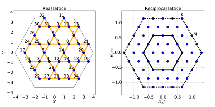
Figure S1: (Color online): 36d simulation cluster (left) and its reciprocal lattice (right) used in the computation of the extended phase diagram. The solid and the dotted lines in reciprocal space show the first and the extended Brillouin zones respectively. The high symmetry points, $K$ and $M$, of the latter have been indicated.

Figure S2: (Color online): Structure factors for magnetically ordered phases $\sqrt{3}\times\sqrt{3}$ (left) and $q=0$ (right) computed from Exact Diagonalization at $J_{z}=0.1$ $J_{2}=-0.1$ and $J_{z}=0.1$ $J_{2}=0.1$ respectively. For $J_{2}<0$, the intensity is maximum at the $K$ points of the extended Brillouin zone and for $J_{2}>0$ it is maximum at the $M$ points.

IV Fidelity profiles for $J_{2}$ scans

In Fig. 3 of the main text, we showed the phase diagram for the kagome antiferromagnet in the parameter space of $J_{z}$ and $J_{2}$, for the model Hamiltonian,

$$H[J_{z},J_{2}] = \Big{(}\sum_{\langle i,j\rangle}S^{x}_{i}S^{x}_{j}+S^{y}_{i}S^{y}_{j}+J_{z}S^{z}_{i}S^{z}_{j}\Big{)}+J_{2}\Big{(}\sum_{\langle\langle i,j\rangle\rangle}S^{x}_{i}S^{x}_{j}+S^{y}_{i}S^{y}_{j}+J_{z}S^{z}_{i}S^{z}_{j}\Big{)}$$ (S18)

$$= H^{\textrm{nn}}_{XXZ}[J_{z}]+J_{2}H^{\textrm{nnn}}_{XXZ}[J_{z}]$$

where $\langle i,j\rangle$ and $\langle\langle i,j\rangle\rangle$ denote the nearest neighbor (nn) and next-nearest-neighbor (nnn) sites respectively.

Our estimates of the phase boundaries were based on the measuring fidelity of the ground state wavefunction $\psi(J_{z},J_{2})$, by scanning in the $J_{2}$ direction (keeping $J_{z}$ fixed),

$$f(J_{z},J_{2})\equiv\Big{|}\langle\psi(J_{z},J_{2}-\Delta J_{2}/2)|\psi(J_{z},J_{2}+\Delta J_{2}/2)\rangle\Big{|}$$ (S19)

where $\Delta J_{2}$ is the step size. Dips in the fidelity profile indicate the existence of phase transitions.

Our results for representative $J_{z}$, with $\Delta J_{2}=0.01$ are shown in Fig. S3. We observe that there are prominent dips for $J_{2}<0$ and $J_{2}\approx 0$ and only a marginal one for $J_{2}>0$. The location of of both the leftmost and rightmost dips increases in $|J_{2}|$ on increasing $J_{z}$, this corresponds to the appearance of the wedge in the kagome phase diagram in Fig. 3. Prominently, the dip at $J_{2}\approx 0$ is present for all $J_{z}$ shown.

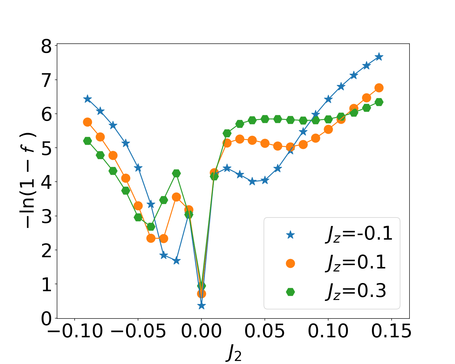
Figure S3: (Color online) Fidelity scans along the $J_{2}$ axis for different values of $J_{z}$. The fidelity is evaluated for ground state wavefunctions at parameter values which differ by $\Delta J_{2}=0.01$ (keeping $J_{z}$ fixed). The spreading location of the leftmost and rightmost dips (increase in $|J_{2}|$), as $J_{z}$ is increased, corresponds to the wedge feature in the kagome phase diagram.

V Ferromagnet and boundaries shared with adjoining phases

In this section of the supplement, we discuss certain aspects of the ferromagnetic (FM) region reported in Fig. 3 of the phase diagram and the phase boundaries it shares with its adjoining phases.

Moving along the direction of $J_{z}<-0.5$ lifts the exponential degeneracy to favor the fully polarized sector. Therefore, in the $S_{z}=0$ sector, the energy density (energy per site) is minimized by the phase separated FM state which has half the system ($N$ sites) maximally polarized up ($S_{z}=N/2$) and the other half maximally polarized down ($S_{z}=-N/2$). This can be proven analytically, since the fully polarized state simultaneously generates the minimal possible energy for all four terms of the Hamiltonian ($XXZ0$ of the triangles made of nearest neighbor bonds, $J_{2}XXZ0$ of the triangles made of next nearest neighbor bonds, $(J_{z}+1/2)\sum_{\langle i,j\rangle}S_{i}^{z}S_{j}^{z}$ and $J_{2}(J_{z}+1/2)\sum_{\langle\langle i,j\rangle\rangle}S_{i}^{z}S_{j}^{z}$) for $J_{2}\geq 0$. Phase separation results in a domain wall which costs absolute energy but, in the TDL, costs zero energy per site for short-ranged Hamiltonians such as ours. While it is possible there are other states with the same energy density but lower absolute energy for a finite system, we see no evidence of this.

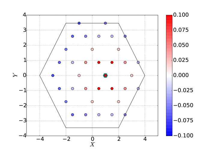
Figure S4: (Color online): ZZ component of the real space spin-spin correlation function (with respect to a reference site) in the $S_{z}=0$ ground state at $J_{z}=-0.7$, $J_{2}=0$. The cyan hexagon marks the lattice site with respect to which the correlation function is computed. The color represents the correlation strength (red - ferromagnetic, blue antiferromagnetic correlations).

While a large enough simulation will exhibit emergent phase separation, finite size effects dominate in a small ED calculation. Nonetheless, in most (but not all) of the region $J_{z}<-0.5,J_{2}>0$ we see clear phase separation in the spin-spin correlation function such as at $J_{z}=-0.7$, $J_{2}=0.0$, see Fig. S4.

Let us now consider the lines separating the $q=0$ and FM (the vertical line $J_{z}=-1/2$ for $J_{2}\geq 0$) and the $\sqrt{3}\times\sqrt{3}$ and FM regions, the latter calculated to be,

$$|J_{z}|=\frac{(\frac{1}{2}+|J_{2}|)}{(1-|J_{2}|)}$$ (S20)

Both boundaries can be understood by comparing the semiclassical energy of the unprojected magnetically ordered states with that of the FM. For example, the energy associated with four nearest neighbor and four next nearest neighbor bonds emanating from a single site in the FM state is $-4|J_{z}|+4|J_{2}||J_{z}|$ in comparison to $4(-1/2)-4|J_{2}|$ for the unprojected coplanar $\sqrt{3}\times\sqrt{3}$ state. The phase boundary of these two phases is shown by the solid line in Fig. 3 of the main text and corresponds to Eq. (S20). Similarly, the $q=0$ energy is higher than the FM for $J_{z}<-1/2$ for any $J_{2}>0$. We note that despite involving only semiclassical arguments, the agreement of these phase boundary estimates with those obtained from energy densities calculated from ED, is excellent.

VI Hamiltonian with four coloring exact ground states

We noted that the idea of coloring wavefunctions generally applies to beyond triangular motifs. Here we explicitly write down the Hamiltonian for which the four coloring wavefunction is an exact ground state on lattices with motifs involving four sites (such as the square, checkerboard and pyrochlore lattices). We derive this Hamiltonian for the case of four sites; the extension to the case of lattices with shared four colorable motifs is trivial.

First, define the four colors as,

$$|a\rangle \equiv |\uparrow\rangle+|\downarrow\rangle$$ (S21a)

$$|b\rangle \equiv |\uparrow\rangle+i|\downarrow\rangle$$ (S21b)

$$|c\rangle \equiv |\uparrow\rangle-|\downarrow\rangle$$ (S21c)

$$|d\rangle \equiv |\uparrow\rangle-i|\downarrow\rangle$$ (S21d)

Then define the states,

$$|1\rangle \equiv |\downarrow\uparrow\uparrow\uparrow\rangle+|\uparrow\downarrow\uparrow\uparrow\rangle+|\uparrow\uparrow\downarrow\uparrow\rangle+|\uparrow\uparrow\uparrow\downarrow\rangle$$ (S22a)

$$|2\rangle \equiv |\uparrow\uparrow\downarrow\downarrow\rangle+|\uparrow\downarrow\uparrow\downarrow\rangle+|\uparrow\downarrow\downarrow\uparrow\rangle+|\downarrow\uparrow\uparrow\downarrow\rangle+|\downarrow\uparrow\downarrow\uparrow\rangle+|\downarrow\downarrow\uparrow\uparrow\rangle$$ (S22b)

$$|3\rangle \equiv |\uparrow\downarrow\downarrow\downarrow\rangle+|\downarrow\uparrow\downarrow\downarrow\rangle+|\downarrow\downarrow\uparrow\downarrow\rangle+|\downarrow\downarrow\downarrow\uparrow\rangle$$ (S22c)

Then, any Hamiltonian of the form

$$H=\lambda_{1}|1\rangle\langle 1|+\lambda_{2}|2\rangle\langle 2|+\lambda_{3}|3\rangle\langle 3|$$ (S23)

with $\lambda_{1},\lambda_{2},\lambda_{3}\geq 0$ will have the coloring wavefunction $|C\rangle=|a\rangle\otimes|b\rangle....$ as an exact ground state with zero energy as long as one satisfies the constraint of one $a$, $b$, $c$, $d$ each per four-site motif. Here we present the result for $\lambda_{1}=\lambda_{2}=\lambda_{3}=1$, where $H$ is also time reversal invariant.

We used the DiracQ package Wright and Shastry (2013) to simplify the spin algebra and up to an overall scale factor found the Hamiltonian to be,

$$H = \frac{7}{8}+\Big{(}\sum_{i<j}S_{i}^{+}S^{-}_{j}+S^{-}_{i}S^{+}_{j}-\frac{1}{2}S^{z}_{i}S^{z}_{j}\Big{)}+\sum_{i<j,k<l,\text{diff}}S_{i}^{+}S^{+}_{j}S_{k}^{-}S^{-}_{l}-2\;S^{z}_{1}S^{z}_{2}S^{z}_{3}S^{z}_{4}$$ (S24)

where the notation "diff" is used to indicate that all the indices $i,j,k,l$ are distinct.

References

- Anderson (1973) P. Anderson, Materials Research Bulletin 8, 153 (1973).
- Helton et al. (2007) J. S. Helton, K. Matan, M. P. Shores, E. A. Nytko, B. M. Bartlett, Y. Yoshida, Y. Takano, A. Suslov, Y. Qiu, J.-H. Chung, D. G. Nocera, and Y. S. Lee, Phys. Rev. Lett. 98, 107204 (2007).
- Okamoto et al. (2007) Y. Okamoto, M. Nohara, H. Aruga-Katori, and H. Takagi, Phys. Rev. Lett. 99, 137207 (2007).
- Zeng and Elser (1990) C. Zeng and V. Elser, Phys. Rev. B 42, 8436 (1990).
- Singh and Huse (2007) R. R. P. Singh and D. A. Huse, Phys. Rev. B 76, 180407 (2007).
- Ran et al. (2007) Y. Ran, M. Hermele, P. A. Lee, and X.-G. Wen, Phys. Rev. Lett. 98, 117205 (2007).
- Yan et al. (2011) S. Yan, D. A. Huse, and S. R. White, Science 332, 1173 (2011).
- Depenbrock et al. (2012) S. Depenbrock, I. P. McCulloch, and U. Schollwöck, Phys. Rev. Lett. 109, 067201 (2012).
- Iqbal et al. (2013) Y. Iqbal, F. Becca, S. Sorella, and D. Poilblanc, Phys. Rev. B 87, 060405 (2013).
- Jiang et al. (2012) H.-C. Jiang, Z. Wang, and L. Balents, Nat. Phys. 8, 902 (2012).
- Clark et al. (2013) B. K. Clark, J. M. Kinder, E. Neuscamman, G. K.-L. Chan, and M. J. Lawler, Phys. Rev. Lett. 111, 187205 (2013).
- Tay and Motrunich (2011) T. Tay and O. I. Motrunich, Phys. Rev. B 84, 020404 (2011).
- He et al. (2017) Y.-C. He, M. P. Zaletel, M. Oshikawa, and F. Pollmann, Phys. Rev. X 7, 031020 (2017).
- Liao et al. (2017) H. J. Liao, Z. Y. Xie, J. Chen, Z. Y. Liu, H. D. Xie, R. Z. Huang, B. Normand, and T. Xiang, Phys. Rev. Lett. 118, 137202 (2017).
- He and Chen (2015) Y.-C. He and Y. Chen, Phys. Rev. Lett. 114, 037201 (2015).
- Changlani and Läuchli (2015) H. J. Changlani and A. M. Läuchli, Phys. Rev. B 91, 100407 (2015).
- Yao et al. (2015) N. Y. Yao, M. P. Zaletel, D. M. Stamper-Kurn, and A. Vishwanath, ArXiv e-prints (2015), arXiv:1510.06403 [cond-mat.str-el] .
- Yamamoto et al. (2014) D. Yamamoto, G. Marmorini, and I. Danshita, Phys. Rev. Lett. 112, 127203 (2014).
- Sellmann et al. (2015) D. Sellmann, X.-F. Zhang, and S. Eggert, Phys. Rev. B 91, 081104 (2015).
- Chernyshev and Zhitomirsky (2014) A. L. Chernyshev and M. E. Zhitomirsky, Phys. Rev. Lett. 113, 237202 (2014).
- Götze and Richter (2015) O. Götze and J. Richter, Phys. Rev. B 91, 104402 (2015).
- Kumar et al. (2014) K. Kumar, K. Sun, and E. Fradkin, Phys. Rev. B 90, 174409 (2014).
- Kumar et al. (2016) K. Kumar, H. J. Changlani, B. K. Clark, and E. Fradkin, Phys. Rev. B 94, 134410 (2016).
- Essafi et al. (2016) K. Essafi, O. Benton, and L. D. C. Jaubert, Nat. Commun. 7, 10297 (2016).
- Momoi and Suzuki (1992) T. Momoi and M. Suzuki, Journal of the Physical Society of Japan 61, 3732 (1992).
- Batista (2009) C. D. Batista, Phys. Rev. B 80, 180406 (2009).
- Shastry and Sutherland (1981) B. S. Shastry and B. Sutherland, Physica B+C 108, 1069 (1981).
- Majumdar and Ghosh (1969) C. K. Majumdar and D. K. Ghosh, Journal of Mathematical Physics 10, 1388 (1969).
- Klein (1982) D. J. Klein, Journal of Physics A: Mathematical and General 15, 661 (1982).
- Affleck et al. (1987) I. Affleck, T. Kennedy, E. H. Lieb, and H. Tasaki, Phys. Rev. Lett. 59, 799 (1987).
- Wen (2003) X.-G. Wen, Phys. Rev. Lett. 90, 016803 (2003).
- Kitaev (2003) A. Kitaev, Annals of Physics 303, 2 (2003).
- Wang et al. (2017) H. Wang, H. J. Changlani, Y. Wan, and O. Tchernyshyov, Phys. Rev. B 95, 144425 (2017).
- Harris et al. (1992) A. B. Harris, C. Kallin, and A. J. Berlinsky, Phys. Rev. B 45, 2899 (1992).
- Henley (2009) C. L. Henley, Phys. Rev. B 80, 180401 (2009).
- Huse and Rutenberg (1992) D. A. Huse and A. D. Rutenberg, Phys. Rev. B 45, 7536 (1992).
- Chalker et al. (1992) J. T. Chalker, P. C. W. Holdsworth, and E. F. Shender, Phys. Rev. Lett. 68, 855 (1992).
- Sachdev (1992) S. Sachdev, Phys. Rev. B 45, 12377 (1992).
- Cépas and Ralko (2011) O. Cépas and A. Ralko, Phys. Rev. B 84, 020413 (2011).
- Castelnovo et al. (2005) C. Castelnovo, C. Chamon, C. Mudry, and P. Pujol, Phys. Rev. B 72, 104405 (2005).
- Baxter (1970) R. J. Baxter, Journal of Mathematical Physics 11, 784 (1970).
- Bergman et al. (2008) D. L. Bergman, C. Wu, and L. Balents, Phys. Rev. B 78, 125104 (2008).
- Leung and Elser (1993) P. W. Leung and V. Elser, Phys. Rev. B 47, 5459 (1993).
- Läuchli et al. (2011) A. M. Läuchli, J. Sudan, and E. S. Sørensen, Phys. Rev. B 83, 212401 (2011).
- Kolley et al. (2015) F. Kolley, S. Depenbrock, I. P. McCulloch, U. Schollwöck, and V. Alba, Phys. Rev. B 91, 104418 (2015).
- Iqbal et al. (2012) Y. Iqbal, F. Becca, and D. Poilblanc, New Journal of Physics 14, 115031 (2012).
- Jiang et al. (2016) S. Jiang, P. Kim, J. H. Han, and Y. Ran, arXiv preprint arXiv:1610.02024 (2016).
- Läuchli and Moessner (2015) A. M. Läuchli and R. Moessner, ArXiv e-prints (2015), arXiv:1504.04380 [cond-mat.quant-gas] .
- Rousochatzakis et al. (2008) I. Rousochatzakis, A. M. Läuchli, and F. Mila, Phys. Rev. B 77, 094420 (2008).
- Kondev and Henley (1996) J. Kondev and C. L. Henley, Nuclear Physics B 464, 540 (1996).
- Khemani et al. (2012) V. Khemani, R. Moessner, S. A. Parameswaran, and S. L. Sondhi, Phys. Rev. B 86, 054411 (2012).
- Wan and Gingras (2016) Y. Wan and M. J. P. Gingras, Phys. Rev. B 94, 174417 (2016).
- Wright and Shastry (2013) J. G. Wright and B. S. Shastry, ArXiv e-prints (2013), arXiv:1301.4494 [cond-mat.str-el] .
- Chan and Duan (2012) Y.-H. Chan and L.-M. Duan, New Journal of Physics 14, 113039 (2012).
- Normand and Nussinov (2014) B. Normand and Z. Nussinov, Phys. Rev. Lett. 112, 207202 (2014).
- Hermele et al. (2004) M. Hermele, M. P. A. Fisher, and L. Balents, Phys. Rev. B 69, 064404 (2004).
- Huse and Elser (1988) D. A. Huse and V. Elser, Phys. Rev. Lett. 60, 2531 (1988).
- Changlani et al. (2009) H. J. Changlani, J. M. Kinder, C. J. Umrigar, and G. K.-L. Chan, Phys. Rev. B 80, 245116 (2009).
- Neuscamman et al. (2011) E. Neuscamman, H. Changlani, J. Kinder, and G. K.-L. Chan, Phys. Rev. B 84, 205132 (2011).