Laguerre Functions and Their Applications to tempered Fractional Differential Equations on Infinite Intervals

Abstract.

Tempered fractional derivatives originated from the tempered fractional diffusion equations (TFDEs) modeled on the whole space $\mathbb{R}$ (see [23]). For numerically solving TFDEs, two kinds of generalized Laguerre functions were defined and some important properties were proposed to establish the approximate theory. The related prototype tempered fractional differential problems was proposed and solved as the guidance. TFDEs are numerically solved by two domains Laguerre spectral method and the numerical experiments show some properties of the TFDEs and verify the efficiency of the spectral scheme.

1. Introduction

The normal diffusion equation $\partial_{t}p(x,t)=\partial_{x}^{2}p(x,t)$ can be derived from the Brownian motion which describes the particle’s random walks. Over the last few decades, a large body of literature has demonstrated that anomalous diffusion, in which the mean square variance grows faster (super-diffusion) or slower (sub-diffusion) than in a Gaussian process, offers a superior fit to experimental data observed in many important practical applications, e.g., in physical science [14, 17, 18, 19], finance [11, 16, 25], biology [13, 5] and hydrology [4, 8, 9]. The anomalous diffusion equation takes the form

$$\partial^{\nu}_{t}p(x,t)=\partial_{x}^{\mu}p(x,t),$$ (1.1)

where $0<\nu\leq 1$ and $0<\mu<2$ (cf. [17] for a review on this subject), whose solution exhibits heavy tails, i.e., power law decays at infinity. In order to ”temper” the power law decay, the authors of [23] applied an exponential factor $e^{-\lambda|x|}$ to the particle jump density, and showed that the Fourier transform of the tempered probability density function $p(x,t)$ takes the form

$${\mathscr{F}}[p](\omega,t)=e^{-[pA_{+}^{\mu,\lambda}(\omega)+qA_{-}^{\mu,\lambda}(\omega)]Dt},\quad 0<\mu<2,$$

where $0\leq p\leq 1,~{}q=1-p$, $D$ is a constant and

$$A_{\pm}^{\mu,\lambda}(\omega):=\begin{cases}(\lambda\pm i\omega)^{\mu}-\lambda^{\mu},&0<\mu<1,\\ (\lambda\pm i\omega)^{\mu}-\lambda^{\mu}-\pm i\omega\mu\lambda^{\mu-1},&1<\mu<2.\end{cases}$$

Moreover, they defined tempered fractional derivative operators $\partial_{\pm,x}^{\mu,\lambda}$ through Fourier transform: $\mathscr{F}{[\partial_{\pm,x}^{\mu,\lambda}u]}(\omega)=A_{\pm}^{\mu,\lambda}(\omega)\mathscr{F}[u](\omega)$, and derived the tempered fractional diffusion equation (TFDE):

$$\partial_{t}u(x,t)=(-1)^{k}C_{T}\{p\partial_{+,x}^{\mu,\lambda}+q\partial_{-,x}^{\mu,\lambda}\}u(x,t),\quad\mu\in(k-1,k),~{}k=1,2.$$ (1.2)

It has been argued that tempered anomalous diffusion models have advantages over the normal dissuasion models in some applications of geophysics [15, 31] and finance [6].

Note that the fractional operators $\partial_{\pm,x}^{\mu,\lambda}u$ was defined by Fourier transform and without any explicit formula. Sabzikar etc bring in alternative form of the tempered fractional integrals and derivatives (TFI/Ds) (we respectively rewrite in Definition 2.2 and Definition 2.3) which derived by applying the inverse Fourier transform,

$${}{\rm D}_{\pm}^{\mu,\lambda}u(x)=\mathscr{F}^{-1}\big{[}(\lambda\pm i\omega)^{\mu}\mathscr{F}{[u]}(\omega)\big{]}(x).$$

Then, the original fractional operator, defined by Fourier transform, can be rewritten as the following equivalent explicit form,

$$\partial_{\pm,x}^{\mu,\lambda}u=\begin{cases}{}{\rm D}_{\pm}^{\mu,\lambda}u-\lambda^{\mu}u,&0<\mu<1,\\ {}{\rm D}_{\pm}^{\mu,\lambda}u-\pm\mu\lambda^{\mu-1}\partial_{x}u-\lambda^{\mu}u,&1<\mu<2.\end{cases}$$ (1.3)

It is a challenging task to numerically solve the tempered fractional diffusion equation (1.2), due particularly to (i) the non-local nature of tempered fractional derivatives; and (ii) the unboundedness of the domain. In [23], the authors used a finite-difference approach on a truncated domain. In [29], the authors considered tempered derivatives on a finite interval and derived an efficient Petrov-Galerkin method for solving tempered fractional ODEs by using the eigenfunctions of tempered fractional Sturm-Liouville problems. In [12], the authors used Laguerre functions to approximate the substantial fractional ODEs, which are similar to those we consider in Section 3, on the half line. In order to avoid the difficulty of assigning boundary conditions at the truncated boundary, we shall deal with the unbounded domain directly in this paper.

Since the tempered factional diffusion equation is derived from the random walk on the whole line, one is tempted to use Hermite polynomials/functions which are suitable for many problems on the whole line [26]. Unfortunately, due to the exponential factor $e^{\lambda|x|}$ in the tempered fractional derivatives, Hermite polynomials/functions are not suitable basis functions. Instead, as we will show in Section 3, properly defined generalized Laguerre functions (GLFs) enjoy particularly simple form under the action of tempered fractional derivatives, just as the relations between generalized Jacobi functions and usual fractional derivatives [7]. Hence, the main goal of this paper is to design efficient spectral methods using GLFs to solve the tempered fractional diffusion equation (1.2) in various situations. However, Laguerre polynomials/functions are mutually orthogonal on the half line, how do we use them to deal with (1.2) on the whole line? We shall first consider special cases of (1.2) with $p=1,\,q=0$ or $p=0,\,q=1$. In these cases, we can reduce (1.2) to the half line, and the GLFs can be naturally used. For the general case, we shall employ a two-domain spectral-element method, and use GLFs as basis functions on each subdomain.

by choosing there are two main tools for the numerical implementation: 1. Hermite spectral method; 2. Domain decomposition method. In this paper, we select the later because there are no good relations between the Hermite basis functions and tempered fractional derivative be found at present, and the structure of the TFDs in (2.24) motivates us to develop the new generalized Laguerre functions to utilize the two domain generalized Laguerre spectral elements method as the tool for approximation. Particularly, as a special case, the half line tempered fractional diffusion is also interesting to investigate, which is tailored for Laguerre spectral method.

The Laguerre spectral method and its development are credited to Funaro [funaro1991estimates], Guo and Shen [guo2000laguerre], Guo et al. [Guo2006generalizedLaguerre], Guo and Zhang [GuoZhang2005new], and Xu and Guo [GuoXu2002laguerre]. They developed the approximations using the Laguerre and generalized Laguerre polynomials, and provided the spectral methods for the half line. Guo and Ma [GuoMa2001composite], Guo and Zhang [GuoZhang2007GLF], and Shen [shen2000stable], studied the approximations by using the Laguerre and generalized Laguerre functions, and the related spectral methods. Recently, Zhang and Guo [30], and Guo and Zhang [GuoZhangC2013laguerre] considered the more general Laguerre approximations and the Laguerre quasi-orthogonal approximations, which are specially appropriate for problems of non-standard type, and exterior problems. Base on the previous works and the special structure of the tempered derivative, we developed a new generalized Laguerre spectral to solving the tempered fractional diffusion (1.2) and its special case. In detail, two kinds of generalized Laguerre functions (GLFs) were proposed in which the traditional Laguerre functions was modified to derive the closed relation with TFI/Ds.

The rest of the paper is organized as follows. In the next section, we introduce the definition of the tempered fractional derivative. Then, in order to extend the whole line TFDs into the general interval, the following is to investigate the more general tempered fractional derivative, especially for the tempered fractional derivatives defined on the half line $\mathbb{R}^{+}$ which coincide with the original whole line tempered fractional derivative by imposing some adequate requirements. Section 4 and section 5 are devoted to the development of the two kinds of generalized Laguerre functions, and their closed relations with TFDs. Some approximation results were exhibited to show the approximate ability. Moreover, for the purpose of the guidance on how to handle the tempered fractional differential equation, we investigate some prototype tempered fractional problems. Finally, we use the established theory to solve a special case in section 7 and the general tempered fractional diffusion problem in section 8 .

The rest of the paper is organized as follows. In the next section, we present the definition of the tempered fractional derivatives, and recall some useful properties of Laguerre polynomials. In Sections 3, we define two classes of generalized Laguerre functions, study their approximation properties, and apply them for solving simple one sided tempered fractional equations. In Section 7, we develop a spectral-Galerkin method for solving a tempered fractional diffusion equation on the half line. Finally, we present a spectral-Galerkin method for solving the tempered fractional diffusion equation on the whole line in Section 8. Some concluding remarks are given in the last section.

2. Preliminaries

Let $\mathbb{N}$ and $\mathbb{R}$ be respectively the sets of positive integers and real numbers. We further denote

$${\mathbb{N}}_{0}:=\{0\}\cup{\mathbb{N}},\;\;{\mathbb{R}}^{+}:=\{x\in{\mathbb{R}}:x>0\},\;\;{\mathbb{R}}^{-}:=\{x\in{\mathbb{R}}:x<0\},\;\;\mathbb{R}_{0}^{\pm}:=\mathbb{R}^{\pm}\cup\{0\}.$$ (2.1)

2.1. Usual (non-tempered) fractional integrals and derivatives

Recall the definitions of the fractional integrals and fractional derivatives in the sense of Riemann-Liouville (see e.g., [21]).

Definition 2.1 (Riemann-Liouville fractional integrals and derivatives).

For $a,b\in{\mathbb{R}}$ or $a=-\infty,b=\infty,$ and $\mu\in{\mathbb{R}}^{+},$ the left and right fractional integrals are respectively defined as

$${}_{a}{\rm I}_{x}^{\mu}u(x)=\frac{1}{\Gamma(\mu)}\int_{a}^{x}\frac{u(y)}{(x-y)^{1-\mu}}{\rm d}y,\;\;{}_{x}{\rm I}_{b}^{\mu}u(x)=\frac{1}{\Gamma(\mu)}\int_{x}^{b}\frac{u(y)}{(y-x)^{1-\mu}}{\rm d}y,\;\;\;x\in\Lambda:=(a,b).$$ (2.2)

For real $s\in[k-1,k)$ with $k\in{\mathbb{N}},$ the left-sided Riemann-Liouville fractional derivative (LRLFD) of order $s$ is defined by

$${{}_{a}}{\rm D}_{x}^{s}u(x)=\frac{1}{\Gamma(k-s)}\frac{d^{k}}{dx^{k}}\int_{a}^{x}\frac{u(y)}{(x-y)^{s-k+1}}{\rm d}y,\;\;\;x\in\Lambda,$$ (2.3)

and the right-sided Riemann-Liouville fractional derivative (RRLFD) of order $s$ is defined by

$${{}_{x}}{\rm D}_{b}^{s}u(x)=\frac{(-1)^{k}}{\Gamma(k-s)}\frac{d^{k}}{dx^{k}}\int_{x}^{b}\frac{u(y)}{(y-x)^{s-k+1}}{\rm d}y,\;\;\;x\in\Lambda.$$ (2.4)

From the above definitions, it is clear that for any $k\in{\mathbb{N}}_{0},$

$${{}_{x}}{\rm D}_{b}^{k}=(-1)^{k}{}{\rm D}^{k},\quad{{}_{a}}{\rm D}_{x}^{k}={}{\rm D}^{k},\;\;\;{\rm where}\;\;\;{}{\rm D}^{k}:=\frac{d^{k}}{dx^{k}}.$$ (2.5)

Therefore, we can express the RLFD as

$${{}_{a}}{\rm D}_{x}^{s}u(x)={}{\rm D}^{k}\big{\{}{}_{a}{\rm I}_{x}^{k-s}u(x)\big{\}};\quad\;{{}_{x}}{\rm D}_{b}^{s}u(x)=(-1)^{k}{}{\rm D}^{k}\big{\{}{}_{x}{\rm I}_{b}^{k-s}u(x)\big{\}}.$$ (2.6)

According to [10, Thm. 2.14], we have that for any finite $a$ and any $v\in L^{1}(\Lambda),$ and real $s\geq 0,$

$${{}_{a}}{\rm D}_{x}^{s}\,{}_{a}{\rm I}_{x}^{s}f(x)=f(x),\quad\text{a.e. in}\;\;\Lambda.$$ (2.7)

Note that by commuting the integral and derivative operators in (B.5), we define the Caputo fractional derivatives:

$${}_{a}^{C}{\rm D}_{x}^{s}u(x)={}_{a}{\rm I}_{x}^{k-s}\big{\{}{}{\rm D}^{k}u(x)\big{\}};\quad\;{}_{x}^{C}{\rm D}_{b}^{s}u(x)=(-1)^{k}{}_{x}{\rm I}_{b}^{k-s}\big{\{}{}{\rm D}^{k}u(x)\big{\}}.$$ (2.8)

For an affine transform $x=\lambda t,~{}\lambda>0$, on account of

$${}_{a}{\rm I}_{t}^{\mu}v(\lambda t) =\frac{1}{\Gamma(\mu)}\int_{a}^{t}\frac{v(\lambda s)}{(t-s)^{1-\mu}}ds=\frac{\lambda^{-\mu}}{\Gamma(\mu)}\int_{a}^{t}\frac{v(\lambda s)}{(\lambda t-\lambda s)^{1-\mu}}\lambda ds$$

$$=\frac{\lambda^{-\mu}}{\Gamma(\mu)}\int_{\lambda a}^{x}\frac{v(y)}{(x-y)^{1-\mu}}dy=\lambda^{-\mu}{}_{\lambda a}{\rm I}_{x}^{\mu}v(x),$$

and $\frac{\rm d}{{\rm d}t}=\lambda\frac{\rm d}{{\rm d}x},$ we derive from Definition D.1 that

$${}_{a}{\rm I}_{t}^{\mu}v(\lambda t)=\lambda^{-\mu}{}_{\lambda a}{\rm I}_{x}^{\mu}v(x),\quad{{}_{a}}{\rm D}_{t}^{s}v(\lambda t)=\lambda^{s}{{}_{\lambda a}}{\rm D}_{x}^{s}v(x),\quad s,\mu,\lambda>0.$$ (2.9)

Similarly, we have the following identities for the right fractional derivative:

$${}_{t}{\rm I}_{b}^{\mu}v(\lambda t)=\lambda^{-\mu}{}_{t}{\rm I}_{\lambda b}^{\mu}v(x),\quad{{}_{t}}{\rm D}_{b}^{s}v(\lambda t)=\lambda^{s}{{}_{x}}{\rm D}_{\lambda b}^{s}v(x),\quad s,\mu,\lambda>0.$$ (2.10)

2.2. Tempered fractional integrals and derivatives on ${\mathbb{R}}$

Recently, Sabzikar et al. [23, (19)-(23)] introduced the tempered fractional integrals and derivatives on the whole line.

Definition 2.2 (Tempered fractional integrals).

For $\lambda\in{\mathbb{R}}^{+}_{0}$, the left tempered fractional integral of a suitable function $u(x)$ of order $\mu\in{\mathbb{R}}^{+}$ is defined by

$${}_{-\infty}{\rm I}_{x}^{\mu,\lambda}u(x)=\frac{1}{\Gamma(\mu)}\int_{-\infty}^{x}\frac{e^{-\lambda(x-y)}}{(x-y)^{1-\mu}}\,u(y)\,{\rm d}y,\quad x\in\mathbb{R},$$ (2.11)

and the right tempered fractional integral of order $\mu\in{\mathbb{R}}^{+}$ is defined by

$${}_{x}{\rm I}_{\infty}^{\mu,\lambda}u(x)=\frac{1}{\Gamma(\mu)}\int^{\infty}_{x}\frac{e^{-\lambda(y-x)}}{(y-x)^{1-\mu}}\,u(y)\,{\rm d}y,\quad x\in\mathbb{R}.$$ (2.12)

It is evident that by (B.1) and (2.11)-(2.12), we have

$${}_{-\infty}{\rm I}_{x}^{\mu}={}_{-\infty}{\rm I}_{x}^{\mu,0},\quad{}_{x}{\rm I}_{\infty}^{\mu}={}_{x}{\rm I}_{\infty}^{\mu,0},$$ (2.13)

and

$${}_{-\infty}{\rm I}_{x}^{\mu,\lambda}u(x)=e^{-\lambda x}{}_{-\infty}{\rm I}_{x}^{\mu}\big{\{}e^{\lambda x}u(x)\big{\}},\quad{}_{x}{\rm I}_{\infty}^{\mu,\lambda}u(x)=e^{\lambda x}{}_{x}{\rm I}_{\infty}^{\mu}\big{\{}e^{-\lambda x}u(x)\big{\}}.$$ (2.14)

As shown in [23], the tempered fractional derivative can be characterized by its Fourier transform. Recall that, for any $u\in L^{2}({\mathbb{R}}),$ its Fourier transform and inverse Fourier transform are defined by

$${\mathscr{F}}[u](\omega)=\int_{-\infty}^{\infty}u(x)e^{-{\rm i}\omega x}\,{\rm d}x;\quad u(x)={\mathscr{F}}^{-1}\big{[}{\mathscr{F}}[u](\omega)\big{]}(x)=\frac{1}{2\pi}\int_{-\infty}^{\infty}{\mathscr{F}}[u](\omega)e^{{\rm i}\omega x}\,{\rm d}\omega.$$ (2.15)

There holds the well-known Parseval’s identity:

$$\int_{-\infty}^{\infty}u(x)\,\bar{v}(x)\,{\rm d}x=\frac{1}{2\pi}\int_{-\infty}^{\infty}{\mathscr{F}}[u](\omega)\,\overline{{\mathscr{F}}[v]}(\omega)\,{\rm d}\omega,$$ (2.16)

where $\bar{v}$ is the complex conjugate of $v$. Let $H(x)$ be the Heaviside function, i.e., $H(x)=1$ for $x\geq 0,$ and vanishing for all $x<0.$ Then we can reformulate the left tempered fractional integral as

$$\begin{split}{}_{-\infty}{\rm I}_{x}^{\mu,\lambda}u(x)&=\frac{1}{\Gamma(\mu)}\int_{0}^{\infty}y^{\mu-1}e^{-\lambda y}u(x-y)\,{\rm d}y=\frac{1}{\Gamma(\mu)}\int_{-\infty}^{\infty}y^{\mu-1}e^{-\lambda y}H(y)\,u(x-y)\,{\rm d}y\\ &=\big{(}{K}\ast u\big{)}(x),\quad{\rm where}\;\;\;{K}(x):=x^{\mu-1}e^{-\lambda x}H(x)/{\Gamma(\mu)}.\end{split}$$ (2.17)

Note that ${K}(x)$ is related to the particle jump density (cf. [23, (8)]). Using the formula: ${\mathscr{F}}[K](\omega)={(\lambda+{\rm i}\omega)^{-\mu}},$ and the convolution property of Fourier transform (see, e.g., [24, 27]), we derive

$${\mathscr{F}}[{}_{-\infty}{\rm I}_{x}^{\mu,\lambda}u](\omega)={\mathscr{F}}[K\ast u](\omega)={\mathscr{F}}[K](\omega)\,{\mathscr{F}}[u](\omega)={(\lambda+{\rm i}\omega)^{-\mu}}{\mathscr{F}}[u](\omega).$$ (2.18)

Similarly, the Fourier transform of the right tempered fractional integral is

$${\mathscr{F}}[{}_{x}{\rm I}_{\infty}^{\mu,\lambda}u](\omega)={(\lambda-{\rm i}\omega)^{-\mu}}{\mathscr{F}}[u](\omega).$$ (2.19)

In view of (2.18)-(2.19), Sabzikar et al. [23] then introduced the left and right tempered fractional derivatives as follows.

Definition 2.3 (Tempered fractional derivatives).

For $\lambda\in{\mathbb{R}}^{+}_{0}$, the left and right tempered fractional derivatives of order $\mu\in{\mathbb{R}}^{+}$ of a suitable function $u(x),$ are defined by

$${\mathscr{F}}\big{[}{{}_{-\infty}}{\rm D}_{x}^{\mu,\lambda}u\big{]}(\omega)=(\lambda+{\rm i}\omega)^{\mu}{\mathscr{F}}[u](\omega),\quad{\mathscr{F}}\big{[}{{}_{x}}{\rm D}_{\infty}^{\mu,\lambda}u\big{]}(\omega)=(\lambda-{\rm i}\omega)^{\mu}{\mathscr{F}}[u](\omega),$$ (2.20)

that is, for any $x\in{\mathbb{R}}$,

$${{}_{-\infty}}{\rm D}_{x}^{\mu,\lambda}u(x)={\mathscr{F}^{-1}}\big{[}{(\lambda+{\rm i}\omega)^{\mu}}{\mathscr{F}}[u](\omega)\big{]}(x),\quad{{}_{x}}{\rm D}_{\infty}^{\mu,\lambda}u(x)={\mathscr{F}^{-1}}\big{[}{(\lambda-{\rm i}\omega)^{\mu}}{\mathscr{F}}[u](\omega)\big{]}(x).$$ (2.21)

Introduce the space

$$W^{\mu,2}_{\lambda}(\mathbb{R}):=\Big{\{}u\in L^{2}(\mathbb{R})\,:~{}\int_{\mathbb{R}}(\lambda^{2}+\omega^{2})^{\mu}\,\big{|}\mathscr{F}[u](\omega)\big{|}^{2}{\rm d}\omega<\infty\Big{\}},\quad\mu,\lambda\in{\mathbb{R}}^{+}.$$ (2.22)

Thanks to the Parseval’s identity (2.16), the above tempered fractional derivatives are well-defined for any $u\in W^{\mu,2}_{\lambda}(\mathbb{R}).$ Moreover, one verifies from (2.18)-(2.21) that

$${}_{-\infty}{\rm I}_{x}^{\mu,\lambda}{{}_{-\infty}}{\rm D}_{x}^{\mu,\lambda}u(x)=u(x),\;\;\;\;{}_{x}{\rm I}_{\infty}^{\mu,\lambda}{{}_{x}}{\rm D}_{\infty}^{\mu,\lambda}u(x)=u(x),\quad\forall\,u\in W^{\mu,2}_{\lambda}(\mathbb{R});\;\;$$ (2.23)

$${{}_{-\infty}}{\rm D}_{x}^{\mu,\lambda}{}_{-\infty}{\rm I}_{x}^{\mu,\lambda}u(x)=u(x),\;\;\;\;{{}_{x}}{\rm D}_{\infty}^{\mu,\lambda}{}_{x}{\rm I}_{\infty}^{\mu,\lambda}u(x)=u(x),\quad\forall\,u\in L^{2}(\mathbb{R}).$$

Similar to (2.14), we have the following explicit representations.

Proposition 2.1.

For any $u\in W^{\mu,2}_{\lambda}(\mathbb{R}),$ with $\lambda\in{\mathbb{R}}^{+}_{0}$, the left and right tempered fractional derivatives of order $\mu\in[k-1,k)$ with $k\in{\mathbb{N}},$ have the explicit representations:

$${{}_{-\infty}}{\rm D}_{x}^{\mu,\lambda}u(x)=e^{-\lambda x}{{}_{-\infty}}{\rm D}_{x}^{\mu}\big{\{}e^{\lambda x}u(x)\big{\}},\quad{{}_{x}}{\rm D}_{\infty}^{\mu,\lambda}u(x)=e^{\lambda x}{{}_{x}}{\rm D}_{\infty}^{\mu}\big{\{}e^{-\lambda x}u(x)\big{\}},$$ (2.24)

where ${{}_{-\infty}}{\rm D}_{x}^{\mu}$ and ${{}_{x}}{\rm D}_{\infty}^{\mu}$ are the Riemann-Liouville fractional derivative operators in Definition D.1. Alternatively, we have

$$\begin{split}{{}_{-\infty}}{\rm D}_{x}^{\mu,\lambda}u(x)&=({}{\rm D}+\lambda)^{k}\,\big{\{}{}_{-\infty}{\rm I}_{x}^{k-\mu,\lambda}u(x)\big{\}}=({}{\rm D}+\lambda)^{k}\,\big{\{}e^{-\lambda x}{}_{-\infty}{\rm I}_{x}^{k-\mu}\big{\{}e^{\lambda x}u(x)\big{\}}\big{\}};\\ {{}_{x}}{\rm D}_{\infty}^{\mu,\lambda}u(x)&=({}{\rm D}-\lambda)^{k}\,\big{\{}{}_{x}{\rm I}_{\infty}^{k-\mu}u(x)\big{\}}=({}{\rm D}-\lambda)^{k}\,\big{\{}e^{\lambda x}{}_{x}{\rm I}_{\infty}^{k-\mu}\big{\{}e^{-\lambda x}u(x)\big{\}}\big{\}}.\end{split}$$ (2.25)

Proof.

Using the properties of Fourier transform: ${\mathscr{F}}[e^{-\lambda x}D^{k}v]=(\lambda+{\rm i}\omega)^{k}{\mathscr{F}}[e^{-\lambda x}v],$ and

$$\begin{split}{\mathscr{F}}\big{[}e^{-\lambda x}&{{}_{-\infty}}{\rm D}_{x}^{\mu}\big{\{}e^{\lambda x}u(x)\big{\}}\big{]}(\omega)={\mathscr{F}}\big{[}e^{-\lambda x}{}{\rm D}^{k}{}_{-\infty}{\rm I}_{x}^{k-\mu}\big{\{}e^{\lambda x}u(x)\big{\}}\big{]}(\omega)\\ &=(\lambda+{\rm i}\omega)^{k}{\mathscr{F}}\big{[}e^{-\lambda x}{}_{-\infty}{\rm I}_{x}^{k-\mu}\big{\{}e^{\lambda x}u(x)\big{\}}\big{]}(\omega)\\ &=(\lambda+{\rm i}\omega)^{k}{\mathscr{F}}\big{[}{}_{-\infty}{\rm I}_{x}^{k-\mu,\lambda}u(x)\big{]}(\omega)=(\lambda+{\rm i}\omega)^{\mu}{\mathscr{F}}[u](\omega).\end{split}$$ (2.26)

This verifies (2.20)-(2.21). Similarly, we can derive the second representation of ${{}_{x}}{\rm D}_{\infty}^{\mu,\lambda}u$ in (2.24).

The alternative form (2.25) can be derived by induction. Here we only verify the left tempered derivative.

• For $\mu\in[0,1)$, we derive from (2.14) and (2.24) that

  $${{}_{-\infty}}{\rm D}_{x}^{\mu,\lambda}u(x) =e^{-\lambda x}{{}_{-\infty}}{\rm D}_{x}^{\mu}\big{\{}e^{\lambda x}u(x)\big{\}}=e^{-\lambda x}\,{\rm D}{}_{-\infty}{\rm I}_{x}^{1-\mu}\big{\{}e^{\lambda x}u(x)\big{\}}$$

  $$=e^{-\lambda x}\,{\rm D}\big{[}e^{\lambda x}{}_{-\infty}{\rm I}_{x}^{1-\mu,\lambda}\big{\{}e^{\lambda x}u(x)\big{\}}\big{]}=({\rm D}+\lambda)\big{\{}{}_{-\infty}{\rm I}_{x}^{1-\mu,\lambda}\big{\{}e^{\lambda x}u(x)\big{\}}\big{\}},$$

  which verifies the identity with $k=1.$

• For $\mu\in{[k-2,k-1)}$, we assume that (2.25) is true. We next verify the identity holds for $\mu\in[k-1,k)$.

  $$\begin{split}&({}{\rm D}+\lambda)^{k}\,\big{\{}{}_{-\infty}{\rm I}_{x}^{k-\mu,\lambda}u(x)\big{\}}=({}{\rm D}+\lambda)({}{\rm D}+\lambda)^{k-1}\,\big{\{}e^{-\lambda x}{}_{-\infty}{\rm I}_{x}^{k-\mu}\big{\{}e^{\lambda x}u(x)\big{\}}\big{\}}\\ &~{}~{}=({}{\rm D}+\lambda)\big{\{}e^{-\lambda x}{{}_{-\infty}}{\rm D}_{x}^{\mu-1}\big{\{}e^{\lambda x}u(x)\big{\}}\big{\}}=e^{-\lambda x}{{}_{-\infty}}{\rm D}_{x}^{\mu}\big{\{}e^{\lambda x}u(x)\big{\}}={{}_{-\infty}}{\rm D}_{x}^{\mu,\lambda}u(x).\end{split}$$

This ends the proof. ∎

We collect below some useful properties (cf. [23]).

Lemma 2.1.

Given $\lambda>0$ and $\mu\in[k-1,k),~{}k\in{\mathbb{N}}$, the tempered fractional derivative

$${{}_{-\infty}}{\rm D}_{x}^{\mu,\lambda}u(x)={{}_{-\infty}}{\rm D}_{x}^{k,\lambda}{}_{-\infty}{\rm I}_{x}^{k-\mu,\lambda}u(x),\quad{{}_{x}}{\rm D}_{\infty}^{\mu,\lambda}u(x)={{}_{x}}{\rm D}_{\infty}^{k,\lambda}{}_{x}{\rm I}_{\infty}^{k-\mu,\lambda}u(x).$$ (2.27)

In addition, we have

$${}_{-\infty}{\rm I}_{x}^{\mu+\nu,\lambda}u(x)={}_{-\infty}{\rm I}_{x}^{\mu,\lambda}{}_{-\infty}{\rm I}_{x}^{\nu,\lambda}u(x),\quad\quad{}_{x}{\rm I}_{\infty}^{\mu+\nu,\lambda}u(x)={}_{x}{\rm I}_{\infty}^{\mu,\lambda}{}_{x}{\rm I}_{\infty}^{\nu,\lambda}u(x),$$ (2.28)

$${{}_{-\infty}}{\rm D}_{x}^{\mu+\nu,\lambda}u(x)={{}_{-\infty}}{\rm D}_{x}^{\mu,\lambda}{{}_{-\infty}}{\rm D}_{x}^{\nu,\lambda}u(x),\quad{{}_{x}}{\rm D}_{\infty}^{\mu+\nu,\lambda}u(x)={{}_{x}}{\rm D}_{\infty}^{\mu,\lambda}{{}_{x}}{\rm D}_{\infty}^{\nu,\lambda}u(x),$$ (2.29)

$$({{}_{-\infty}}{\rm D}_{x}^{\mu,\lambda}u,v)=(u,{{}_{x}}{\rm D}_{\infty}^{\mu,\lambda}v),\qquad\qquad\qquad({{}_{x}}{\rm D}_{\infty}^{\mu,\lambda}u,v)=(u,{{}_{-\infty}}{\rm D}_{x}^{\mu,\lambda}v),$$ (2.30)

where $\mu,\nu\geq 0$.

Remark 2.1.

For a suitable function $f(x),~{}x\in\mathbb{R}^{+}$, its reflection $g(y)=f(-y),~{}y\in\mathbb{R}^{-}$ satisfies

$${}_{-\infty}{\rm I}_{y}^{\mu,\lambda}g(y)= \frac{e^{-\lambda y}}{\Gamma(\mu)}\int_{-\infty}^{y}e^{\lambda\tau}(y-\tau)^{\mu-1}f(-\tau){\rm d}\tau\overset{t=-\tau}{=}\frac{e^{-\lambda y}}{{\Gamma(\mu)}}\int^{\infty}_{-y}e^{-\lambda t}(y+t)^{\mu-1}f(t)\rm{\rm d}t$$ (2.31)

$$\overset{x=-y}{=} \frac{e^{\lambda x}}{{\Gamma(\mu)}}\int^{\infty}_{x}e^{-\lambda t}(t-x)^{\mu-1}f(t){\rm d}t={}_{x}{\rm I}_{\infty}^{\mu,\lambda}f(x).$$

Hence, we can use (2.27) and derivative relation $\dfrac{{\rm d}^{k}}{{\rm d}y^{k}}=(-1)^{k}\dfrac{{\rm d}^{k}}{{\rm d}x^{k}}$ to obtain the tempered derivative relation

$${{}_{-\infty}}{\rm D}_{y}^{\mu,\lambda}f(-y)={{}_{x}}{\rm D}_{\infty}^{\mu,\lambda}f(x),\quad y=-x,~{}x\in\mathbb{R}^{+}.$$ (2.32)

∎

2.3. Tempered fractional integrals and derivatives on the half line

Let $H(x)$ be the Heaviside function as before. For any function $u(x)$ defined on the half line ${\mathbb{R}}^{+}=(0,\infty),$ we define its zero extension as $\tilde{u}(x):=u(x)H(x)$ for $x\in{\mathbb{R}}.$ It is straightforward to extend the tempered fractional integral to the half line ${\mathbb{R}}^{+}=(0,\infty):$

$${}_{0}{\rm I}_{x}^{\mu,\lambda}u(x):={}_{-\infty}{\rm I}_{x}^{\mu,\lambda}\big{\{}\tilde{u}(x)\big{\}}=\frac{1}{\Gamma(\mu)}\int_{0}^{x}\frac{e^{-\lambda(x-y)}}{(x-y)^{1-\mu}}\,u(y)\,{\rm d}y=e^{-\lambda x}{}_{0}{\rm I}_{x}^{\mu}\big{\{}e^{\lambda x}u(x)\big{\}},\;\;x\in\mathbb{R}^{+},$$ (2.33)

which preserves the property (2.18).

Similarly, for $\lambda\in{\mathbb{R}}^{+}$ and $\mu\in[k-1,k)$ with $k\in\mathbb{N}$, we define

$${{}_{0}}{\rm D}_{x}^{\mu,\lambda}{{u(x)}}:=e^{-\lambda x}{{}_{0}}{\rm D}_{x}^{\mu}\big{\{}e^{\lambda x}{u(x)}\big{\}},\quad x\in{\mathbb{R}}^{+}.$$ (2.34)

Using the property: ${{}_{0}}{\rm D}_{x}^{\mu}=D^{k}{}_{0}{\rm I}_{x}^{k-\mu},$ one verifies from (2.33) that

$${{}_{0}}{\rm D}_{x}^{\mu,\lambda}{{u(x)}} =e^{-\lambda x}{}{\rm D}^{k}\big{\{}e^{\lambda x}{{}_{0}{\rm I}_{x}^{k-\mu,\lambda}{{u}}(x)}\big{\}}=e^{-\lambda x}{}{\rm D}^{k}\big{\{}e^{\lambda x}{{}_{-\infty}{\rm I}_{x}^{k-\mu,\lambda}{\tilde{u}}(x)}\big{\}}$$ (2.35)

$$=e^{-\lambda x}{{}_{-\infty}}{\rm D}_{x}^{\mu}\big{\{}e^{\lambda x}{\tilde{u}(x)}\big{\}},\quad x\in{\mathbb{R}}^{+}.$$

From Proposition 2.1, we conclude that if $\tilde{u}(x)\in W^{\mu,2}_{\lambda}(\mathbb{R})$, then (2.34) defines the left tempered derivative in the sense of Definition 2.3 on the half line. More precisely, there hold

$${{}_{-\infty}}{\rm D}_{x}^{\mu,\lambda}{{\tilde{u}(x)}}=e^{-\lambda x}{{}_{-\infty}}{\rm D}_{x}^{\mu}\big{\{}e^{\lambda x}{\tilde{u}(x)}\big{\}}={{}_{0}}{\rm D}_{x}^{\mu,\lambda}{{u(x)}},\quad x\in\mathbb{R}^{+},$$ (2.36)

and

$${\mathscr{F}}\big{[}{{}_{-\infty}}{\rm D}_{x}^{\mu,\lambda}{\tilde{u}}\big{]}(\omega)=(\lambda+{\rm i}\omega)^{\mu}{\mathscr{F}}[\tilde{u}](\omega)={\mathscr{F}}\big{[}H(x){{}_{0}}{\rm D}_{x}^{\mu,\lambda}{{u(x)}}\big{]}(\omega).$$ (2.37)

Now the remaining problem is to verify whether $\tilde{u}\in W^{\mu,2}_{\lambda}(\mathbb{R})$. This is the criterion to judge the extended tempered fractional derivative still keep the original definition. Indeed, we can show that for $\mu\in(0,1)$ and real $\lambda>0,$ (2.36)-(2.37) are valid. Applying Fourier transform to the explicit expression of the tempered derivative, we have that

$$\begin{split}{\mathscr{F}}\big{[}e^{-\lambda x}{{}_{-\infty}}{\rm D}_{x}^{\mu}\big{\{}e^{\lambda x}{\tilde{u}(x)}\big{\}}\big{]}(\omega)=&\int_{\mathbb{R}}{}{\rm D}{}_{-\infty}{\rm I}_{x}^{1-\mu}\big{\{}e^{\lambda x}{\tilde{u}(x)}\big{\}}~{}e^{-(\lambda+{\rm i}\omega)x}{\rm d}x\\ =(\lambda+{\rm i}\omega)&\int_{\mathbb{R}}{}_{-\infty}{\rm I}_{x}^{1-\mu}\big{\{}e^{\lambda x}{\tilde{u}(x)}\big{\}}~{}e^{-(\lambda+{\rm i}\omega)x}{\rm d}x\\ \overset{\eqref{Int-exchange}}{=}(\lambda+{\rm i}\omega)&\int_{\mathbb{R}}e^{\lambda x}{\tilde{u}(x)}~{}{}_{x}{\rm I}_{\infty}^{1-\mu}e^{-(\lambda+{\rm i}\omega)x}{\rm d}x\\ =(\lambda+{\rm i}\omega)^{\mu}&{\mathscr{F}}[\tilde{u}](\omega)\overset{\eqref{Temdef2FourierB}}{=}{\mathscr{F}}\big{[}{{}_{-\infty}}{\rm D}_{x}^{\mu,\lambda}{{\tilde{u}(x)}}\big{]}(\omega).\end{split}$$

Then, (2.36)-(2.37) can be deduced from the above and (2.35).

However, if $\mu\geq 1,$ $\tilde{u}(x)$ is not always in $W^{\mu,2}_{\lambda}(\mathbb{R})$. For example, we consider $u(x)=e^{-\lambda x},x>0.$ A direct calculation yields

$${{}_{-\infty}}{\rm D}_{x}^{\mu,\lambda}{\tilde{u}(x)}=\dfrac{x^{-\mu}e^{-\lambda x}}{\Gamma(1-\mu)}H(x),\quad x\in{\mathbb{R}},$$ (2.38)

which implies that $\tilde{u}\not\in W^{\mu,2}_{\lambda}(\mathbb{R})$. Hence, in this case, a naive zero extension of $u$ does not always lead to a tempered fractional derivative as in Definition 2.3. In fact, a smooth zero extension of $u$ is necessary to ensure (2.36) with $\mu\geq 1$. For this purpose, we define the extension $\breve{u}(x)$ of $u$ (such that ${}{\rm D}^{k}u\in L^{2}(\mathbb{R}^{+})$), as

$$\breve{u}(x)=\begin{cases}u(x),\quad&{\rm if}\;\;x>0,\\ 0,\quad&{\rm if}\;\;x<0,\\ \end{cases}\quad\;\;\breve{u}(x)\in C^{k-2}(\mathbb{R}),\quad k\geq 2,$$ (2.39)

which implies

$${}{\rm D}^{j}u(0)=0,\quad j=0,1,\cdots,k-2.$$ (2.40)

For example, one verifies that

$$\breve{u}(x)={}_{-\infty}{\rm I}_{x}^{k-1}\big{\{}H(x){{}{\rm D}^{k-1}u}(x)\big{\}},\quad x\in\mathbb{R},$$ (2.41)

provides such an extension of $u(x)$. With this at our disposal, we can show (2.36)-(2.37) hold with $\breve{u}$ in place of $\tilde{u}.$

Proposition 2.2.

Given real $\lambda>0$ and $\mu\in[k-1,k)$ with integer $k\geq 2,$ let $D^{k}u\in L^{2}(\mathbb{R}^{+})$ and $\breve{u}$ be a zero extension given in (2.39). Then we have

$${{}_{-\infty}}{\rm D}_{x}^{\mu,\lambda}{{\breve{u}(x)}}={{}_{0}}{\rm D}_{x}^{\mu,\lambda}{{u(x)}},\;\;x\in\mathbb{R}^{+},\quad{\mathscr{F}}\big{[}{{}_{-\infty}}{\rm D}_{x}^{\mu,\lambda}{\breve{u}}\big{]}(\omega)={\mathscr{F}}\big{[}H(x){{}_{0}}{\rm D}_{x}^{\mu,\lambda}{{u(x)}}\big{]}(\omega).$$ (2.42)

Proof.

Using the relation between the Remann-Liouville and Caputo fractional derivatives in (B.10), we can obtain that

$${{}_{0}}{\rm D}_{x}^{\mu,\lambda}{{u}(x)}=e^{-\lambda x}{{}_{0}}{\rm D}_{x}^{\mu}\left\{e^{\lambda x}{u}(x)\right\}{:=}u_{1}(x)+u_{2}(x)+u_{3}(x),$$ (2.43)

where

$$u_{1}(x):=e^{-\lambda x}{}_{0}{\rm I}_{x}^{k-\mu}{}{\rm D}^{k}\{e^{\lambda x}u\},\quad u_{2}(x):=\frac{{}{\rm D}^{k-1}(e^{\lambda x}u)\big{|}_{x=0}}{\Gamma(k-\mu)}~{}x^{k-1-\mu}e^{-\lambda x},\quad$$

$$u_{3}(x):=\sum_{j=0}^{k-2}\frac{{}{\rm D}^{j}(e^{\lambda x}u)\big{|}_{x=0}}{\Gamma(1+j-\mu)}~{}x^{j-\mu}e^{-\lambda x}.$$

Note that by (2.40), $u_{3}(x)\equiv 0.$ On the other hand, by definition (cf. (2.20)),

$${\mathscr{F}}[{{}_{-\infty}}{\rm D}_{x}^{\mu,\lambda}{\breve{u}}](\omega)=(\lambda+{\rm i}\omega)^{\mu}{\mathscr{F}}[\breve{u}](\omega),$$

so it suffices to show

$${\mathscr{F}}\big{[}H(x){{}_{0}}{\rm D}_{x}^{\mu,\lambda}{{u(x)}}\big{]}(\omega)=(\lambda+{\rm i}\omega)^{\mu}{\mathscr{F}}[\breve{u}](\omega).$$ (2.44)

A direct calculation leads to

$$\begin{split}\mathscr{F}[{H}(x)u_{1}(x)](\omega)&=\int_{0}^{\infty}{}_{0}{\rm I}_{x}^{k-\mu}{}{\rm D}^{k}\{e^{\lambda x}u(x)\}~{}e^{-(\lambda+{\rm i}\omega)x}{\rm d}x\\ &\overset{\eqref{Int-exchange}}{=}\int_{0}^{\infty}{}{\rm D}^{k}\{e^{\lambda x}u(x)\}~{}{}_{x}{\rm I}_{\infty}^{k-\mu}e^{-(\lambda+{\rm i}\omega)x}{\rm d}x\\ &{=}(\lambda+{\rm i}\omega)^{\mu-k}\int_{0}^{\infty}{}{\rm D}^{k}\{e^{\lambda x}u(x)\}e^{-(\lambda+{\rm i}\omega)x}{\rm d}x\\ &\overset{\eqref{extendcondition}}{=}(\lambda+{\rm i}\omega)^{\mu-k}[(\lambda+{\rm i}\omega)^{k}~{}\mathscr{F}[\breve{u}](\omega)-u^{(k-1)}(0)],\end{split}$$

and

$$\begin{split}\mathscr{F}[{H}(x)u_{2}(x)]&{=}\frac{u^{(k-1)}(0)}{\Gamma(k-\mu)}\int_{0}^{\infty}x^{k-\mu-1}e^{-(\lambda+{\rm i}\omega)x}{\rm d}x\\ &{=}\frac{u^{(k-1)}(0)}{\Gamma(k-\mu)}(\lambda+{\rm i}\omega)^{\mu-k}\int_{0}^{\infty}((\lambda+{\rm i}\omega)x)^{k-\mu-1}e^{-(\lambda+{\rm i}\omega)x}\,{\rm d}(\lambda+{\rm i}\omega)x\\ &{=}(\lambda+{\rm i}\omega)^{\mu-k}{u}^{(k-1)}(0).\end{split}$$

Thus, the property (2.44) follows directly from (2.43) and the above identities. ∎

2.4. Laguerre polynomials and some useful formulas

For any $a\in{\mathbb{R}}$ and $j\in{\mathbb{N}}_{0},$ we recall that the rising factorial in the Pochhammer symbol and the Gamma function have the relation:

$$(a)_{0}=1;\;\;\;(a)_{j}:=a(a+1)\cdots(a+j-1)=\frac{\Gamma(a+j)}{\Gamma(a)},\;\;{\rm for}\;\;j\geq 1.$$ (2.45)

Recall the hypergeometric function (cf. [1]):

$${}_{1}F_{1}(a;b;x)=\sum_{j=0}^{\infty}\frac{(a)_{j}}{(b)_{j}}\frac{x^{j}}{j!},\;\;\;a,b,x\in{\mathbb{R}}^{+},\;\;-b\not\in{\mathbb{N}}_{0}.$$ (2.46)

If $b-a>0,$ then ${}_{1}F_{1}(a;b;x)$ is absolutely convergent for all $x\in\mathbb{R}.$ If $a$ is a negative integer, then it reduces to a polynomial.

The Laguerre polynomial with parameter $\alpha>-1$ is defined as in Szegö [28, (5.3.3)]:

$$L_{n}^{(\alpha)}(x)=\frac{(\alpha+1)_{n}}{n!}~{}{}_{1}F_{1}\big{(}-n;\alpha+1;x\big{)},\;\;\;n\geq 1,\;\;x\in{\mathbb{R}}^{+},$$ (2.47)

and $L_{0}^{(\alpha)}(x)\equiv 1.$ Note that

$$L_{n}^{(\alpha)}(0)=\dfrac{(\alpha+1)_{n}}{n!},$$ (2.48)

and the Laguerre polynomials (with $\alpha>-1$) are orthogonal with respect to the weight function $x^{\alpha}e^{-x},$ namely,

$$\int_{0}^{\infty}{L}_{n}^{(\alpha)}(x)~{}{L}_{m}^{(\alpha)}(x)~{}x^{\alpha}e^{-x}\,{\rm d}x=\gamma_{n}^{\alpha}\,\delta_{mn},\quad\gamma_{n}^{\alpha}=\frac{\Gamma(n+\alpha+1)}{\Gamma(n+1)}.$$ (2.49)

They are eigenfunctions of the Sturm-Liouville problem:

$$x^{-\alpha}e^{x}\partial_{x}\big{(}x^{\alpha+1}e^{-x}\partial_{x}L_{n}^{(\alpha)}(x)\big{)}+\lambda_{n}L_{n}^{(\alpha)}(x)=0,\quad\lambda_{n}=n.$$ (2.50)

We have the following relations:

$$L_{n}^{(\alpha)}(x)=\partial_{x}L_{n}^{(\alpha)}(x)-\partial_{x}L_{n+1}^{(\alpha)}(x),$$ (2.51)

$$x\partial_{x}L_{n}^{(\alpha)}(x)=nL_{n}^{(\alpha)}(x)-(n+\alpha)L_{n-1}^{(\alpha)}(x),$$ (2.52)

$$\partial_{x}L_{n}^{(\alpha)}(x)=-L_{n-1}^{(\alpha+1)}(x)=-\sum_{k=0}^{n-1}L_{k}^{(\alpha)}(x).$$ (2.53)

In particular, for $\alpha=-k,~{}k=1,2,\ldots$ (See Szegö [28, (5.2.1)]),

$$L_{n}^{(-k)}(x)=(-1)^{k}\frac{\Gamma(n-k+1)}{\Gamma(n+1)}x^{k}L_{n-k}^{(k)}(x),\quad n\geq k.$$

For notational convenience, we denote

$${h}_{n}^{a,b}:=\frac{\Gamma(n+1+a)}{\Gamma(n+1+a-b)}.$$ (2.54)

We present below some formulas related to Laguerre polynomials and fractional integrals and derivatives, which play an important role in the algorithm development and analysis later. We provide their derivations in Appendix B.

Lemma 2.2.

For $\mu\in{\mathbb{R}}^{+},$ we have

$${}_{0}{\rm I}_{x}^{\mu}\{x^{\alpha}L_{n}^{(\alpha)}(x)\}=h^{\alpha,-\mu}_{n}\,x^{\alpha+\mu}L_{n}^{(\alpha+\mu)}(x),\quad\alpha>-1;$$ (2.55)

$${{}_{0}}{\rm D}_{x}^{\mu}\{x^{\alpha}L_{n}^{(\alpha)}(x)\}=h^{\alpha,\mu}_{n}\,x^{\alpha-\mu}L_{n}^{(\alpha-\mu)}(x),\quad\alpha>\mu-1,$$ (2.56)

and

$${}_{x}{\rm I}_{\infty}^{\mu}\{e^{-x}L_{n}^{(\alpha)}(x)\}=e^{-x}L_{n}^{(\alpha-\mu)}(x),\quad\alpha>\mu-1;$$ (2.57)

$${{}_{x}}{\rm D}_{\infty}^{\mu}\{e^{-x}L_{n}^{(\alpha)}(x)\}=e^{-x}L_{n}^{(\alpha+\mu)}(x),\quad\alpha>-1.$$ (2.58)

Moreover, we have that for $k\in\mathbb{N}$ and $\alpha>k-1$,

$${}{\rm D}^{k}\big{\{}x^{\alpha}e^{-x}L_{n}^{(\alpha)}(x)\big{\}}=\frac{\Gamma(n+k+1)}{\Gamma(n+1)}x^{\alpha-k}L^{(\alpha-k)}_{n+k}(x)e^{-x}.$$ (2.59)

3. Generalized Laguerre functions

In this section, we introduce the generalized Laguerre functions (GLFs), and study its approximation properties. In what follows, the operators ${}_{0}{\rm I}_{x}^{\mu,\lambda},{{}_{0}}{\rm D}_{x}^{\mu,\lambda}$ on the half line should be understood as $0$ in place of $-\infty$ in (2.11) and (2.24)-(2.25).

3.1. Definition and properties

We first introduce the GJFs and their associated properties related to tempered fractional integrals/derivatives.

Definition 3.1 (GLFs).

For real $\alpha\in\mathbb{R}$ and $\lambda>0,$ we define the GLFs as

$${\mathcal{L}}^{(\alpha,\lambda)}_{n}{(x)}:=\begin{cases}x^{-\alpha}e^{-\lambda x}\,{L}_{n}^{(-\alpha)}(2\lambda x),\quad\alpha<0,\\ e^{-\lambda x}\,{L}_{n}^{(\alpha)}(2\lambda x),\qquad\quad\,\alpha\geq 0\end{cases}$$ (3.1)

for all $x\in\mathbb{R}^{+}$ and $n\in\mathbb{N}_{0}.$

Remark 3.1.

It’s noteworthy that Zhang and Guo [30] introduce the GJFs

$$\widetilde{\mathscr{L}}_{l}^{(\alpha,\beta)}(x)=\begin{cases}x^{-\alpha}e^{-\frac{\beta}{2}x}L^{(-\alpha)}(\beta x),\quad&\alpha\leq-1,\;\;l\geq\bar{l}_{\alpha}=[-\alpha],\\ e^{-\frac{\beta}{2}x}L_{l}^{(\alpha)}(x),&\alpha>-1,\;\;l\geq\bar{l}_{\alpha}=0,\end{cases}$$ (3.2)

where the scaling factor $\beta>0.$ It is seen that we modified the definition in the range of $0<\alpha<1$ (with $\beta=2\lambda$). This turns out to be essential for the numerical solution of FDEs of order $\mu\in(0,1),$ as we shall see in the subsequent sections. ∎

Compare to the GLFs defined in [30], we split the index at $\alpha=0$ rather than $\alpha=-1$ due to our definition is more reasonable for solving tempered fractional differential problem. Indeed, Zhang and Guo [30] denoted the GLFs by

$$\widetilde{\mathscr{L}}_{l}^{(\alpha,\beta)}(x)=e^{-\frac{\beta}{2}x}\mathscr{L}_{l}^{(\alpha,\beta)}(x),\quad l\geq{\bar{l}_{\alpha}},$$ (3.3)

where

$$\mathscr{L}_{l}^{(\alpha,\beta)}(x)=\begin{cases}x^{-\alpha}L^{(-\alpha,\beta)}(x),\quad&\alpha\leq-1,l\geq\bar{l}_{\alpha}=[-\alpha],\\ L_{l}^{(\alpha,\beta)}(x),&\alpha>-1,l\geq\bar{l}_{\alpha}=0\end{cases}$$

was defined by Guo etc [ben2013jacobi, (4.5)] and $L_{l}^{(\alpha,\beta)}(x)=L_{l}^{(\alpha)}(\beta x)$.

We next present the basic properties of GLFs. Firstly, one verifies readily from the orthogonality (2.49) and Definition 3.1 that for $\alpha\in\mathbb{R}$ and $\lambda>0,$

$$\int_{0}^{\infty}{\mathcal{L}}^{(\alpha,\lambda)}_{n}{(x)}{\mathcal{L}}^{(\alpha,\lambda)}_{m}{(x)}\,x^{\alpha}dx=\gamma_{n}^{{|\alpha|},\lambda}\delta_{nm},\;\;\;\gamma_{n}^{|\alpha|,\lambda}=\frac{\gamma_{n}^{|\alpha|}}{(2\lambda)^{|\alpha|+1}},$$ (3.4)

where $\gamma_{n}^{|\alpha|}$ is defined in (2.49).

We have the following important (left) “tempered” fractional integral and derivative rules.

Lemma 3.1.

For $\mu,\nu,\lambda,x\in{\mathbb{R}}^{+}_{0},$ we have

$${}_{0}{\rm I}_{x}^{\mu,\lambda}{\mathcal{L}}^{(-\nu,\lambda)}_{n}{(x)}=h^{\nu,-\mu}_{n}{\mathcal{L}}^{(-\nu-\mu,\lambda)}_{n}{(x)},$$ (3.5)

$${{}_{0}}{\rm D}_{x}^{\mu,\lambda}{\mathcal{L}}^{(-\nu,\lambda)}_{n}{(x)}=h^{\nu,\mu}_{n}{\mathcal{L}}^{(\mu-\nu,\lambda)}_{n}{(x)},\quad\nu\geq\mu,$$ (3.6)

and

$${{}_{0}}{\rm D}_{x}^{\mu+k,\lambda}{\mathcal{L}}^{(-\mu,\lambda)}_{n}{(x)}=(-2\lambda)^{k}h^{\mu,\mu}_{n}{\mathcal{L}}^{(k,\lambda)}_{n-k}{(x)},\quad n\geq k\in{\mathbb{N}}_{0},$$ (3.7)

where $h^{a,b}_{n}$ is defined in (2.54).

Proof.

We obtain from (2.11) and (2.24)-(2.25) (with replacing $-\infty$ by $0$) that

$${}_{0}{\rm I}_{x}^{\mu,\lambda}{\mathcal{L}}^{(-\nu,\lambda)}_{n}{(x)}=e^{-\lambda x}{}_{0}{\rm I}_{x}^{\mu}\{e^{\lambda x}{\mathcal{L}}^{(-\nu,\lambda)}_{n}{(x)}\}=e^{-\lambda x}{}_{0}{\rm I}_{x}^{\mu}\{x^{\nu}L^{(\nu)}_{n}(2\lambda x)\},$$

and

$${{}_{0}}{\rm D}_{x}^{\mu,\lambda}{\mathcal{L}}^{(-\nu,\lambda)}_{n}{(x)}=e^{-\lambda x}{{}_{0}}{\rm D}_{x}^{\mu}\{e^{\lambda x}{\mathcal{L}}^{(-\nu,\lambda)}_{n}{(x)}\}=e^{-\lambda x}{{}_{0}}{\rm D}_{x}^{\mu}\{x^{\nu}L^{(\nu)}_{n}(2\lambda x)\}.$$

Thus, from (B.11) and Lemma 2.2, we obtain (4.3)-(4.4).

Using (4.4) and the derivative relation (A.5) (with $\alpha=\mu$), we obtain

$${{}_{0}}{\rm D}_{x}^{\mu+k,\lambda}{\mathcal{L}}^{(-\mu,\lambda)}_{n}{(x)} ={{}_{0}}{\rm D}_{x}^{k,\lambda}{{}_{0}}{\rm D}_{x}^{\mu,\lambda}{\mathcal{L}}^{(-\mu,\lambda)}_{n}{(x)}=e^{-\lambda x}{}{\rm D}^{k}\big{\{}e^{\lambda x}h^{\mu,\mu}_{n}{\mathcal{L}}^{(0,\lambda)}_{n}{(x)}\big{\}}$$

$$=h^{\mu,\mu}_{n}\,e^{-\lambda x}{}{\rm D}^{k}\big{\{}L_{n}^{(0)}(2\lambda x)\big{\}}=(-2\lambda)^{k}h^{\mu,\mu}_{n}\,L_{n-k}^{(k)}(2\lambda x)\,e^{-\lambda x}.$$

This leads to (4.5). ∎

Similarly, we have the following rules of the (right) “tempered” fractional integrals and derivatives.

Lemma 3.2.

For $\mu,\nu,\lambda,x\in{\mathbb{R}}^{+}_{0}$, we have

$$\quad{}_{x}{\rm I}_{\infty}^{\mu,\lambda}{\mathcal{L}}^{(\nu,\lambda)}_{n}{(x)}=(2\lambda)^{-\mu}{\mathcal{L}}^{(\nu-\mu,\lambda)}_{n}{(x)},\quad\nu\geq\mu,$$ (3.8)

$${{}_{x}}{\rm D}_{\infty}^{\mu,\lambda}{\mathcal{L}}^{(\nu,\lambda)}_{n}{(x)}=(2\lambda)^{\mu}{\mathcal{L}}^{(\mu+\nu,\lambda)}_{n}{(x)}.$$ (3.9)

Furthermore, let $y=-x$, then

$$\quad{}_{-\infty}{\rm I}_{y}^{\mu,\lambda}{\mathcal{L}}^{(\nu,\lambda)}_{n}{(-y)}=(2\lambda)^{-\mu}{\mathcal{L}}^{(\nu-\mu,\lambda)}_{n}{(-y)},\quad\nu\geq\mu,$$ (3.10)

$${{}_{-\infty}}{\rm D}_{y}^{\mu,\lambda}{\mathcal{L}}^{(\nu,\lambda)}_{n}{(-y)}=(2\lambda)^{\mu}{\mathcal{L}}^{(\mu+\nu,\lambda)}_{n}{(-y)}.$$ (3.11)

Proof.

Identities (5.3) and (5.4) can be easily derived from (B.11), (B.12) and Lemma 2.2. ∎

We highlight the fractional derivative formulas, which play an important role in the forthcoming algorithm and analysis.

Theorem 3.1.

Let $k\in\mathbb{N}$ and $k-\nu\leq 0$,

$${{}_{-\infty}}{\rm D}_{x}^{k,\lambda}\big{\{}{\mathcal{L}}^{(-\nu,\lambda)}_{n}{(x)}\big{\}}=\frac{\Gamma(n+\nu+1)}{\Gamma(n+\nu-k+1)}~{}{\mathcal{L}}^{(k-\nu,\lambda)}_{n}{(x)},$$ (3.12)

$$\qquad{{}_{x}}{\rm D}_{\infty}^{k,\lambda}\big{\{}{\mathcal{L}}^{(-\nu,\lambda)}_{n}{(x)}\big{\}}=(-1)^{k}\frac{\Gamma(n+k+1)}{\Gamma(n+1)}{\mathcal{L}}^{(k-\nu,\lambda)}_{n+k}{(x)}.\qquad$$ (3.13)

Proof.

From Lemma 2.2 and relations

$${{}_{-\infty}}{\rm D}_{x}^{k,\lambda}u=e^{-\lambda x}{}{\rm D}^{k}\big{\{}e^{\lambda x}u\big{\}},\quad{{}_{x}}{\rm D}_{\infty}^{k,\lambda}u=e^{\lambda x}(-1)^{k}{}{\rm D}^{k}\big{\{}e^{-\lambda x}u\big{\}},$$ (3.14)

we obtain that for $k-\nu\leq 0$,

$${{}_{-\infty}}{\rm D}_{x}^{k,\lambda} \big{\{}x^{\nu}{\mathcal{L}}^{(\nu,\lambda)}_{n}{(x)}\big{\}}=e^{-\lambda x}{}{\rm D}^{k}\big{\{}(2\lambda)^{-\nu}(2\lambda x)^{\nu}L^{(\nu)}_{n}(2\lambda x)\big{\}}$$

$$\overset{\eqref{lagupolyderi}}{=} \frac{\Gamma(n+1+\nu)}{\Gamma(n+\nu-k+1)}x^{\nu-k}L^{(\nu-k)}_{n}(2\lambda x)e^{-\lambda x}=\frac{\Gamma(n+1+\nu)}{\Gamma(n+\nu-k+1)}~{}{\mathcal{L}}^{(k-\nu,\lambda)}_{n}{(x)},$$

and

$${{}_{x}}{\rm D}_{\infty}^{k,\lambda}\big{\{}x^{\nu}{\mathcal{L}}^{(\nu,\lambda)}_{n}{(x)}\big{\}}= e^{\lambda x}(-1)^{k}{}{\rm D}^{k}\big{\{}(2\lambda)^{-\nu}(2\lambda x)^{\nu}L^{(\nu)}_{n}(2\lambda x)e^{-2\lambda x}\big{\}}$$ (3.15)

$$\overset{\eqref{lagufunderi}}{=} (-1)^{k}\frac{\Gamma(n+k+1)}{\Gamma(n+1)}x^{\nu-k}L^{(\nu-k)}_{n+k}(2\lambda x)e^{-\lambda x}$$

$$= (-1)^{k}\frac{\Gamma(n+k+1)}{\Gamma(n+1)}~{}{\mathcal{L}}^{(k-\nu,\lambda)}_{n}{(x)}.$$

This ends the proof. ∎

Another attractive property of GLFs is that they are eigenfunctions of Sturm-Liouville problem.

Theorem 3.2.

Let $s,\nu,x\in\mathbb{R}^{+}_{0}$ and $n\in\mathbb{N}_{0}$. Then,

$$\qquad x^{\nu}{{}_{x}}{\rm D}_{\infty}^{s,\lambda}\{x^{s-\nu}{{}_{0}}{\rm D}_{x}^{s,\lambda}\,{\mathcal{L}}^{(-\nu,\lambda)}_{n}{(x)}\}=\lambda_{n,-}^{s,\nu}\,{\mathcal{L}}^{(-\nu,\lambda)}_{n}{(x)},\quad\nu-s\geq 0,$$ (3.16)

and

$$x^{-\nu}{{}_{0}}{\rm D}_{x}^{s,\lambda}\{x^{s+\nu}{{}_{x}}{\rm D}_{\infty}^{s,\lambda}\,{\mathcal{L}}^{(\nu,\lambda)}_{n}{(x)}\}=\lambda_{n,+}^{s,\nu}\,{\mathcal{L}}^{(\nu,\lambda)}_{n}{(x)},\qquad\qquad\,$$ (3.17)

where the corresponding eigenvalues $\lambda_{n,-}^{s,\nu}=(2\lambda)^{s}h_{n}^{\nu,s}$ and $\lambda_{n,+}^{s,\nu}=(2\lambda)^{s}h_{n}^{\nu+s,s}$.

Proof.

Due to (4.4) and (5.4),

$${{}_{0}}{\rm D}_{x}^{s,\lambda}{\mathcal{L}}^{(-\nu,\lambda)}_{n}{(x)}=h^{\nu,s}_{n}{\mathcal{L}}^{(s-\nu,\lambda)}_{n}{(x)},\quad{{}_{x}}{\rm D}_{\infty}^{s,\lambda}{\mathcal{L}}^{(\nu-s,\lambda)}_{n}{(x)}=(2\lambda)^{s}{\mathcal{L}}^{(\nu,\lambda)}_{n}{(x)}.$$

It’s straightforward to obtain that

$$x^{\nu} {{}_{x}}{\rm D}_{\infty}^{s,\lambda}\{x^{s-\nu}{{}_{0}}{\rm D}_{x}^{s,\lambda}\,{\mathcal{L}}^{(-\nu,\lambda)}_{n}{(x)}\}=x^{\nu}{{}_{x}}{\rm D}_{\infty}^{s,\lambda}\{x^{s-\nu}{{}_{0}}{\rm D}_{x}^{s,\lambda}{\mathcal{L}}^{(-\nu,\lambda)}_{n}{(x)}\}$$

$$=h^{\nu,s}_{n}x^{\nu}{{}_{x}}{\rm D}_{\infty}^{s,\lambda}\{x^{s-\nu}{\mathcal{L}}^{(s-\nu,\lambda)}_{n}{(x)}\}=h^{\nu,s}_{n}x^{\nu}{{}_{x}}{\rm D}_{\infty}^{s,\lambda}{\mathcal{L}}^{(\nu-s,\lambda)}_{n}{(x)}=(2\lambda)^{s}h_{n}^{\nu,s}\,{\mathcal{L}}^{(-\nu,\lambda)}_{n}{(x)}.$$

Similarly, we have

$$x^{-\nu} {{}_{0}}{\rm D}_{x}^{s,\lambda}\{x^{s+\nu}{{}_{x}}{\rm D}_{\infty}^{s,\lambda}\,{\mathcal{L}}^{(\nu,\lambda)}_{n}{(x)}\}=x^{-\nu}{{}_{0}}{\rm D}_{x}^{s,\lambda}\{x^{s+\nu}{{}_{x}}{\rm D}_{\infty}^{s,\lambda}{\mathcal{L}}^{(\nu,\lambda)}_{n}{(x)}\}$$

$$=(2\lambda)^{s}x^{-\nu}{{}_{0}}{\rm D}_{x}^{s,\lambda}\{x^{s+\nu}{\mathcal{L}}^{(s+\nu,\lambda)}_{n}{(x)}\}=(2\lambda)^{s}x^{-\nu}{{}_{0}}{\rm D}_{x}^{s,\lambda}{\mathcal{L}}^{(-\nu-s,\lambda)}_{n}{(x)}=(2\lambda)^{s}h_{n}^{\nu+s,s}\,{\mathcal{L}}^{(\nu,\lambda)}_{n}{(x)}.$$

This ends the derivation. ∎

Another attractive property of GLFs is that they are eigenfunctions of Sturm-Liouville problem. To show their relations, we define two types of Sturm-Liouville operators:

$$\mathcal{T}^{2s}_{\nu,-}u:=x^{\nu}{{}_{x}}{\rm D}_{\infty}^{s,\lambda}\{x^{s-\nu}{{}_{0}}{\rm D}_{x}^{s,\lambda}u\},\quad\mathcal{T}^{2s}_{\nu,+}u:=x^{-\nu}{{}_{0}}{\rm D}_{x}^{s,\lambda}\{x^{s+\nu}{{}_{x}}{\rm D}_{\infty}^{s,\lambda}u\}.$$ (3.18)

Combing with Lemma 4.1 and Lemma 5.1, we have that

Theorem 3.3.

Let $s,\nu,x\in\mathbb{R}^{+}_{0}$ and $n\in\mathbb{N}_{0}$. Then,

$$\qquad\mathcal{T}^{2s}_{\nu,-}\,{\mathcal{L}}^{(-\nu,\lambda)}_{n}{(x)}=\lambda_{n,-}^{s,\nu}\,{\mathcal{L}}^{(-\nu,\lambda)}_{n}{(x)},\quad\nu-s\geq 0,$$ (3.19)

and

$$\mathcal{T}^{2s}_{\nu,+}\,{\mathcal{L}}^{(\nu,\lambda)}_{n}{(x)}=\lambda_{n,+}^{s,\nu}\,{\mathcal{L}}^{(\nu,\lambda)}_{n}{(x)}.\qquad\quad\,$$ (3.20)

where $\lambda_{n,-}^{s,\nu}=(2\lambda)^{s}h_{n}^{\nu,s}$ and $\lambda_{n,+}^{s,\nu}=(2\lambda)^{s}h_{n}^{\nu+s,s}$.

Proof.

Due to (4.4) and (5.4),

$${{}_{0}}{\rm D}_{x}^{s,\lambda}{\mathcal{L}}^{(-\nu,\lambda)}_{n}{(x)}=h^{\nu,s}_{n}{\mathcal{L}}^{(s-\nu,\lambda)}_{n}{(x)},\quad{{}_{x}}{\rm D}_{\infty}^{s,\lambda}{\mathcal{L}}^{(\nu-s,\lambda)}_{n}{(x)}=(2\lambda)^{s}{\mathcal{L}}^{(\nu,\lambda)}_{n}{(x)}.$$

It’s straightforward to obtain that

$$\mathcal{T}^{2s}_{\nu,-}{\mathcal{L}}^{(-\nu,\lambda)}_{n}{(x)} =x^{\nu}{{}_{x}}{\rm D}_{\infty}^{s,\lambda}\{x^{s-\nu}{{}_{0}}{\rm D}_{x}^{s,\lambda}{\mathcal{L}}^{(-\nu,\lambda)}_{n}{(x)}\}=h^{\nu,s}_{n}x^{\nu}{{}_{x}}{\rm D}_{\infty}^{s,\lambda}\{x^{s-\nu}{\mathcal{L}}^{(s-\nu,\lambda)}_{n}{(x)}\}$$

$$=h^{\nu,s}_{n}x^{\nu}{{}_{x}}{\rm D}_{\infty}^{s,\lambda}{\mathcal{L}}^{(\nu-s,\lambda)}_{n}{(x)}=(2\lambda)^{s}h_{n}^{\nu,s}\,{\mathcal{L}}^{(-\nu,\lambda)}_{n}{(x)}.$$

Similarly, we have

$$\mathcal{T}^{2s}_{\nu,+}{\mathcal{L}}^{(\nu,\lambda)}_{n}{(x)} =x^{-\nu}{{}_{0}}{\rm D}_{x}^{s,\lambda}\{x^{s+\nu}{{}_{x}}{\rm D}_{\infty}^{s,\lambda}{\mathcal{L}}^{(\nu,\lambda)}_{n}{(x)}\}=(2\lambda)^{s}x^{-\nu}{{}_{0}}{\rm D}_{x}^{s,\lambda}\{x^{s+\nu}{\mathcal{L}}^{(s+\nu,\lambda)}_{n}{(x)}\}$$

$$=(2\lambda)^{s}x^{-\nu}{{}_{0}}{\rm D}_{x}^{s,\lambda}{\mathcal{L}}^{(-\nu-s,\lambda)}_{n}{(x)}=(2\lambda)^{s}h_{n}^{\nu+s,s}\,{\mathcal{L}}^{(\nu,\lambda)}_{n}{(x)}.$$

∎

Remark 3.2.

The above results can be viewed as an extension of the standard Sturm-Liouville problem of generalized Laguerre functions (cf. (A.2)) to the tempered fractional derivative. We derive immediately from (3.19), (3.20) and the Stirling’s formula (see (4.14)) that for fixed $s$ and $\nu$,

$$\lambda_{n,-}^{s,\nu}=\lambda_{n,+}^{s,\nu}=O\big{(}(2\lambda n)^{s}\big{)},\quad n\gg 1.$$

When $s\rightarrow 1$ and $\lambda=1/2$, it recovers the $O(n)$ growth of eigenvalues of the standard Sturm-Liouville problem.∎

3.2. Approximation by GLFs

3.2.1. Approximation by $\big{\{}{\mathcal{L}}^{(\alpha,\lambda)}_{n}{(x)}:~{}\alpha=-\nu<0\big{\}}_{n=0}^{\infty}$.

Denote by $\mathcal{P}_{N}$ the set of all polynomials of degree at most $N$, and define the finite dimensional space

$$\mathcal{F}^{\nu,\lambda}_{N}({\mathbb{R}}^{+}):=\big{\{}x^{\nu}e^{-\lambda x}p(x)\,:\,p\in\mathcal{P}_{N}\big{\}},\quad N\in\mathbb{N}_{0}.$$ (3.21)

Define the $L_{\omega}^{2}({\mathbb{R}}^{+})$ with the inner product and norm:

$$(f,g)_{\omega}:=\int_{{\mathbb{R}}^{+}}f\,\bar{g}\,\omega\,{\rm d}x,\quad\|f\|_{\omega}^{2}=(f,f)_{\omega},$$ (3.22)

where $\omega(x)$ be a generic weight function and $\bar{g}$ is the conjugate of the function $g$. In particular, we omit $\omega$ when $\omega\equiv 1.$

To characterize the approximation errors, we define the non-uniformly weighted Sobolev space

$$A_{\nu,\lambda}^{m}({\mathbb{R}}^{+}):=\Big{\{}u\in L^{2}_{\omega^{-\nu}}({\mathbb{R}}^{+}):{{}_{0}}{\rm D}_{x}^{\nu+k,\lambda}u\in L^{2}_{\omega^{k}}({\mathbb{R}}^{+}),\;k=0,\cdots,m\Big{\}},\quad m\in\mathbb{N}_{0},$$ (3.23)

equipped with the norm and semi-norm

$$\|u\|_{A_{\nu,\lambda}^{m}}:=\Big{(}\|u\|^{2}_{\omega^{-\nu}}+\sum_{k=0}^{m}\|{{}_{0}}{\rm D}_{x}^{\nu+k,\lambda}u\|^{2}_{\omega^{k}}\Big{)}^{{1}/{2}},\quad|u|_{A_{\nu,\lambda}^{m}}:=\|{{}_{0}}{\rm D}_{x}^{\nu+m,\lambda}u\|_{\omega^{m}},$$ (3.24)

where the weight function $\omega^{a}(x)=x^{a}.$

Consider the orthogonal projection $\pi_{N}^{-\nu,\lambda}:\,{L^{2}_{\omega^{-\nu}}}({\mathbb{R}}^{+})\rightarrow\mathcal{F}^{\nu,\lambda}_{N}({\mathbb{R}}^{+})$ defined by

$$(\pi_{N}^{-\nu,\lambda}u-u,~{}\phi)_{\omega^{-\nu}}=0,\quad\forall\phi\in\mathcal{F}^{\nu,\lambda}_{N}({\mathbb{R}}^{+}).$$ (3.25)

Then, by the orthogonality (4.2), $u$ and its $L^{2}$-orthogonal projection can be expanded as

$$u(x)=\sum_{n=0}^{\infty}~{}\hat{u}_{n}{\mathcal{L}}^{(-\nu,\lambda)}_{n}{(x)},\quad(\pi_{N}^{-\nu,\lambda}u)(x)=\sum_{n=0}^{N}~{}\hat{u}_{n}{\mathcal{L}}^{(-\nu,\lambda)}_{n}{(x)},$$ (3.26)

where

$$\hat{u}_{n}=\big{(}u,~{}{\mathcal{L}}_{n}^{(-\nu,\lambda)}\big{)}_{\omega^{-\nu}}\big{/}\gamma^{\nu,\lambda}_{n}.$$

Theorem 3.4.

For $\lambda,\nu>0$, we have that for any $u\in A^{m}_{\nu,\lambda}(\mathbb{R}^{+})$ with $m\leq N+1$,

$$\|\pi_{N}^{-\nu,\lambda}u-u\|_{\omega^{-\nu}}\leq~{}c~{}(2\lambda N)^{-\frac{\nu+m}{2}}~{}\|{{}_{0}}{\rm D}_{x}^{\nu+m,\lambda}u\|_{\omega^{m}},$$ (3.27)

and for any $k\leq m,$

$$\big{\|}{{}_{0}}{\rm D}_{x}^{\nu+k,\lambda}\big{(}\pi_{N}^{-\nu,\lambda}u-u\big{)}\big{\|}_{\omega^{k}}\leq~{}c~{}({2\lambda}N)^{\frac{k-m}{2}}~{}\|{{}_{0}}{\rm D}_{x}^{\nu+m,\lambda}u\|_{\omega^{m}},$$ (3.28)

where $c\approx 1$ for large $N.$

Proof.

By (4.11), we have

$$(u-\pi_{N}^{-\nu,\lambda}u)(x)=\sum_{n=N+1}^{\infty}\,\hat{u}_{n}\,{\mathcal{L}}^{(-\nu,\lambda)}_{n}{(x)}.$$

By the orthogonality (4.2) and (4.5),

$$\big{\|}{{}_{0}}{\rm D}_{x}^{\nu+k,\lambda}{\mathcal{L}}^{(-\nu,\lambda)}_{n}{}\big{\|}^{2}_{\omega^{k}}=(-2\lambda)^{2k}\,(h^{\nu,\nu}_{n})^{2}\int_{0}^{\infty}\big{(}L^{(k)}_{n-k}(2\lambda x)\big{)}^{2}\,e^{-2\lambda x}{\omega^{k}}(x){\rm d}x=(d_{n,k}^{\nu,\lambda})^{2}\gamma_{n-k}^{k,\lambda},$$

where we denoted $d_{n,k}^{\nu,\lambda}:=(2\lambda)^{k}\,h^{\nu,\nu}_{n}$ and used the fact:

$$\int_{0}^{\infty}L^{(m)}_{n-m}(2\lambda x)L^{(k)}_{n-k}(2\lambda x)\,e^{-2\lambda x}\omega^{k}dx=\frac{\gamma_{n-k}^{k}}{(2\lambda)^{k+1}}\delta_{km}=\gamma_{n-k}^{k,\lambda}\delta_{km},$$

Thus we can obtain

$$\|\pi_{N}^{-\nu,\lambda}u-u\|^{2}_{\omega^{-\nu}}=\sum_{n=N+1}^{\infty}(\hat{u}_{n})^{2}\gamma_{n}^{\nu,\lambda},\quad\big{|}\pi_{N}^{-\nu,\lambda}u-u\big{|}^{2}_{A^{k}_{\nu,\lambda}}=\sum_{n=N+1}^{\infty}(\hat{u}_{n}d_{n,k}^{\nu,\lambda})^{2}\gamma_{n-k}^{k,\lambda},$$

$$\big{|}u\big{|}^{2}_{A^{m}_{\nu,\lambda}}=\sum_{n=m}^{\infty}(\hat{u}_{n}d_{n,m}^{\nu,\lambda})^{2}\gamma_{n-m}^{m,\lambda}.$$

Then one verifies readily that

$$\|\pi_{N}^{-\nu,\lambda}u-u\|^{2}_{\omega^{-\nu}} \leq\frac{\gamma_{N+1}^{\nu,\lambda}}{(d_{N+1,m}^{\nu,\lambda})^{2}\gamma_{N+1-m}^{m,\lambda}}\big{|}u\big{|}^{2}_{A^{m}_{\nu,\lambda}},$$

$$\quad\big{|}\pi_{N}^{-\nu,\lambda}u-u\big{|}^{2}_{A^{k}_{\nu,\lambda}} \leq\left(\frac{d_{N+1,k}^{\nu,\lambda}}{d_{N+1,m}^{\nu,\lambda}}\right)^{2}\frac{\gamma_{N+1-k}^{k,\lambda}}{\gamma_{N+1-m}^{m,\lambda}}\big{|}u\big{|}^{2}_{A^{m}_{\nu,\lambda}}.$$

Recall the property of the Gamma function (see [1, (6.1.38)]):

$$\Gamma(x+1)=\sqrt{2\pi}x^{x+1/2}\exp\Big{(}-x+\frac{\theta}{12x}\Big{)},\quad\forall\,x>0,\;\;0<\theta<1.$$ (3.29)

One can then obtain that for any constants $a,b,$ and for $n\geq 1,$ $n+a>1$ and $n+b>1,$

$$\frac{\Gamma(n+a)}{\Gamma(n+b)}\leq\nu_{n}^{a,b}n^{a-b},$$ (3.30)

where

$$\nu_{n}^{a,b}=\exp\Big{(}\frac{a-b}{2(n+b-1)}+\frac{1}{12(n+a-1)}+\frac{(a-b)^{2}}{n}\Big{)}.$$ (3.31)

Therefore,

$$\frac{\gamma_{N+1}^{\nu,\lambda}}{(d_{N+1,m}^{\nu,\lambda})^{2}\gamma_{N+1-m}^{m,\lambda}} =\frac{\Gamma(N+2-m)}{(2\lambda)^{\nu+m}\Gamma(N+2+\nu)}\leq(2\lambda)^{-\nu-m}\nu_{n}^{2-m,2+\nu}N^{-\nu-m},$$

$$\left(\frac{d_{N+1,k}^{\nu,\lambda}}{d_{N+1,m}^{\nu,\lambda}}\right)^{2}\frac{\gamma_{N+1-k}^{k,\lambda}}{\gamma_{N+1-m}^{m,\lambda}} =\frac{(2\lambda)^{k}\Gamma(N+2-m)}{(2\lambda)^{m}\Gamma(N+2-k)}<(2\lambda)^{k-m}\nu_{n}^{2-m,2-k}N^{k-m},$$

where $\nu_{n}^{2-m,2+\nu}\approx 1$ and $\nu_{n}^{2-m,2-k}\approx 1$ for fixed $m$ and $n\geq N\gg 1$. Then (4.12)-(4.13) follow. ∎

3.2.2. Approximation by $\big{\{}{\mathcal{L}}^{(\alpha,\lambda)}_{n}{(x)}:~{}\alpha=\nu\geq 0\big{\}}_{n=0}^{\infty}$.

Introduce the non-uniformly weighted Sobolev space:

$$B_{\nu,\lambda}^{r}(\mathbb{R}^{+}):=\Big{\{}u\in L^{2}_{\omega^{\nu}}({\mathbb{R}}^{+}):{{}_{x}}{\rm D}_{\infty}^{s,\lambda}u\in L^{2}_{\omega^{\nu+s}}({\mathbb{R}}^{+}),\;0\leq s\leq r\Big{\}},\quad r\in\mathbb{R}^{+}_{0},$$ (3.32)

endowed with norm and semi-norm

$$\|u\|_{B_{\nu,\lambda}^{r}}:=\Big{(}\|u\|^{2}_{\omega^{\nu}}+|u|^{2}_{B_{\nu,\lambda}^{r}}\Big{)}^{{1}/{2}},\quad|u|_{B_{\nu}^{r}}:=\|{{}_{x}}{\rm D}_{\infty}^{\nu+r,\lambda}u\|_{\omega^{\nu+r}}.$$ (3.33)

Consider the orthogonal projection $\Pi_{N}^{\nu,\lambda}:~{}{L^{2}_{\omega^{\nu}}}({\mathbb{R}}^{+})\rightarrow\mathcal{F}^{0,\lambda}_{N}({\mathbb{R}}^{+}),$ defined by

$$\big{(}\Pi_{N}^{\nu,\lambda}u-u,~{}\phi\big{)}_{\omega^{\nu}}=0,\quad\forall\phi\in\mathcal{F}^{0,\lambda}_{N}({\mathbb{R}}^{+}),\quad\nu>-1,$$ (3.34)

Theorem 3.5.

Let $\lambda,r,\nu>0$. For any $u\in B^{r}_{\nu,\lambda}({\mathbb{R}}^{+})$ with $0\leq s\leq r\leq N,$ we have

$$\big{\|}{{}_{x}}{\rm D}_{\infty}^{s,\lambda}\big{\{}\Pi_{N}^{\nu,\lambda}u-u\big{\}}\big{\|}_{\omega^{\nu+s}}\leq~{}c~{}({2\lambda}{N})^{\frac{s-r}{2}}~{}\|{{}_{x}}{\rm D}_{\infty}^{r,\lambda}u\|_{\omega^{\nu+r}},$$ (3.35)

where $c\approx 1$ for large $N.$

Proof.

Note that by definition,

$$u-\Pi_{N}^{\nu,\lambda}u=\sum_{n=N+1}^{\infty}~{}\hat{u}_{n}{\mathcal{L}}_{n}^{(\nu,\lambda)}(x),\quad\hat{u}_{n}=\big{(}u,~{}{\mathcal{L}}_{n}^{(\nu,\lambda)}\big{)}_{\omega^{\nu}}\big{/}\gamma^{\nu,\lambda}_{n}.$$

Then by (5.4), and the orthgogonality,

$$\|{{}_{x}}{\rm D}_{\infty}^{s,\lambda}{\mathcal{L}}^{(\nu,\lambda)}_{n}{}\|^{2}_{\omega^{\nu+s}}=\|{\mathcal{L}}^{(\nu+s,\lambda)}_{n}{}\|^{2}_{\omega^{\nu+s}}=\gamma_{n}^{\nu+s,\lambda},$$

we can derive

$$\big{|}\Pi_{N}^{\nu,\lambda}u-u\big{|}^{2}_{B^{s}_{\nu,\lambda}} =\|\sum_{n=N+1}^{\infty}\hat{u}_{n}(2\lambda)^{s}{\mathcal{L}}^{(\nu+s,\lambda)}_{n}{}\|^{2}_{\omega^{\nu+s}}=\sum_{n=N+1}^{\infty}(\hat{u}_{n})^{2}(2\lambda)^{2s}\gamma_{n}^{\nu+s,\lambda},$$

$$\big{|}u\big{|}^{2}_{B^{r}_{\nu+r,\lambda}} =\|\sum_{n=0}^{\infty}\hat{u}_{n}(2\lambda)^{r}{\mathcal{L}}^{(\nu+r,\lambda)}_{n}{\|}^{2}_{\omega^{\nu+r}}=\sum_{n=0}^{\infty}(\hat{u}_{n})^{2}(2\lambda)^{2r}\gamma_{n}^{\nu+r,\lambda}.$$

Then,

$$\big{|}\Pi_{N}^{\nu,\lambda}u-u\big{|}^{2}_{B^{s}_{\nu,\lambda}} =\sum_{n=N+1}^{\infty}(\hat{u}_{n})^{2}\gamma_{n}^{\nu+s,\lambda}\leq(2\lambda)^{2s-2r}\frac{\gamma_{N+1}^{\nu+s,\lambda}}{\gamma_{N+1}^{\nu+r,\lambda}}\sum_{n=N+1}^{\infty}(\hat{u}_{n})^{2}\gamma_{n}^{\nu+r,\lambda},$$

where by (4.15)-(4.16), we obtain

$$\dfrac{\gamma_{N+1}^{\nu+s,\lambda}}{\gamma_{N+1}^{\nu+r,\lambda}}=\dfrac{(2\lambda)^{r}\Gamma(N+\nu+s+2)}{(2\lambda)^{s}\Gamma(N+\nu+r+2)}\leq c({2\lambda})^{r-s}N^{s-r}.$$

Consequently, we have

$$\|{{}_{x}}{\rm D}_{\infty}^{s,\lambda}\big{\{}\Pi_{N}^{\nu,\lambda}u-u\big{\}}\|_{\omega^{\nu+s}}\leq~{}c\,({2\lambda}N)^{\frac{s-r}{2}}\,|u|_{B^{r}_{\nu,\lambda}}.$$

This ends the proof. ∎

Remark 3.3.

GLF-I and GLF-II are respectively utilized to derive the Theorem 4.1 and the Theorem 5.1. They are different

The GLF-II was tailored for the right tempered derivative, different from the extended left tempered derivative ${{}_{0}}{\rm D}_{x}^{\mu,\lambda}$, there is no singular point at $x=0$ Furthermore, set $m=0,~{}\nu=0$ in $A^{m}_{\nu,\lambda}$ and $B^{r}_{\nu,\lambda}$ respectively, we have the following more accurate estimate than Theorem 4.1.

Corollary 3.1.

Let $\lambda,r>0$, $\nu>-1$. If $u\in A^{0}_{\nu,\lambda}\cap B^{r}_{0,\lambda}$, then

$$\|\,\pi_{N}^{-\nu,\lambda}u-u\|_{\omega^{-\nu}}\leq~{}c~{}({2\lambda}{N})^{-\frac{\nu+r}{2}}~{}\|{{}_{x}}{\rm D}_{\infty}^{r,\lambda}{{}_{0}}{\rm D}_{x}^{\nu,\lambda}u\|_{\omega^{r}}.$$ (3.36)

In addition, for $0\leq s\leq r$,

$$\|{{}_{x}}{\rm D}_{\infty}^{s,\lambda}{{}_{0}}{\rm D}_{x}^{\nu,\lambda}\big{\{}\pi_{N}^{-\nu,\lambda}u-u\big{\}}\|_{\omega^{s}}\leq~{}c~{}({2\lambda}N)^{\frac{s-r}{2}}~{}\|{{}_{x}}{\rm D}_{\infty}^{r,\lambda}{{}_{0}}{\rm D}_{x}^{\nu,\lambda}u\|_{\omega^{r}}.$$ (3.37)

Proof.

By the direct calculation, we can show that ${{}_{0}}{\rm D}_{x}^{\nu,\lambda}\pi_{N}^{-\nu,\lambda}u=\Pi^{0,\lambda}_{N}u$. Then Corollary 5.2 is the straightforward conclusion of Theorem 5.1. ∎

3.3. A model problem and numerical results

In what follows, we consider the GLF approximation to a model tempered fractional equation of order $s\in[k-1,k)$ with $k\in\mathbb{N}:$

$${{}_{0}}{\rm D}_{x}^{s,\lambda}u(x)=f(x),\;\;x\in\mathbb{R}^{+},\;\;\lambda>0;\;\;u^{(j)}(0)=0,\quad j=0,1,\ldots,k-1,$$ (3.38)

where $f\in L^{2}(\mathbb{R}^{+})$ is a given function. Using the fractional derivative relation (B.9), one can find

$$u(x)={}_{0}{\rm I}_{x}^{s,\lambda}f(x)+\sum\limits_{i=1}^{k}c_{i}\,x^{s-i}e^{-\lambda x},$$

where $\{c_{i}\}$ can be determined by the conditions at $x=0.$ In fact, we have all $c_{i}=0,$ and

$$u(x)={}_{0}{\rm I}_{x}^{s,\lambda}f(x)=\frac{e^{-\lambda x}}{\Gamma(s)}\int_{0}^{x}(x-\tau)^{s-1}e^{\lambda\tau}f(\tau){\rm d}\tau=\frac{x^{s}}{\Gamma(s)}\int_{0}^{1}(1-t)^{s-1}e^{-\lambda(1-t)x}f(xt){\rm d}t.$$ (3.39)

We see that if $f(x)$ is smooth, then $u(x)=x^{s}F(x),$ where $F(x)$ is smoother than $f(x).$ With this understanding, we construct the GLF Petrov-Galerkin approximation as: find $u_{N}\in\mathcal{F}^{s,\lambda}_{N}(\mathbb{R}^{+})$ (defined in (4.6)) such that

$$({{}_{0}}{\rm D}_{x}^{s,\lambda}u_{N},v_{N})=(f,v_{N}),\quad\forall\,v_{N}\in\mathcal{F}^{0,\lambda}_{N}(\mathbb{R}^{+}).$$ (3.40)

We expand $f$ and $u_{N}$ as

$$f(x)=\sum_{n=0}^{\infty}~{}\hat{f}_{n}{\mathcal{L}}^{(0,\lambda)}_{n}{(x)},~{}\quad u_{N}=\sum_{n=0}^{N}~{}\hat{u}_{n}{\mathcal{L}}^{(s,\lambda)}_{n}{(x)}.$$ (3.41)

Using the derivative relation (4.4), we find immediately that $\hat{u}_{n}=\frac{\gamma_{n}^{0,\lambda}}{h_{n}^{s,s}}\hat{f}_{n}$ for $n=0,1,\cdots,N$, which also implies ${{}_{0}}{\rm D}_{x}^{s,\lambda}u_{N}=\pi^{0,\lambda}_{N}f.$

Moreover, we can show that the numerical solution $u_{N}$ is precisely the orthogonal projection in the following sense:

$$(u_{N}-u\,,\,w_{N})_{\omega^{-s}}=0,\quad\forall\,w_{N}\in\mathcal{F}^{s,\lambda}_{N}(\mathbb{R}^{+}).$$ (3.42)

To this end, we first show

$$(u_{N}-u\,,\,{{}_{x}}{\rm D}_{\infty}^{s,\lambda}v_{N})=({{}_{0}}{\rm D}_{x}^{s,\lambda}u_{N}-{{}_{0}}{\rm D}_{x}^{s,\lambda}u,v_{N})=0,\quad\forall\,v_{N}\in\mathcal{F}^{0,\lambda}_{N}(\mathbb{R}^{+}).$$ (3.43)

Indeed, thanks to $u^{(j)}(0)=0$ for $j=0,\ldots,k-1$, we have

$${{}_{0}}{\rm D}_{x}^{s,\lambda}\{u_{N}-u\}=e^{-\lambda x}{{}_{0}}{\rm D}_{x}^{s}\{e^{\lambda x}(u_{N}-u)\}=e^{-\lambda x}{}_{0}{\rm I}_{x}^{k-s}{{}_{0}}{\rm D}_{x}^{k}\{e^{\lambda x}(u_{N}-u)\}.$$

Then,

$$\left({{}_{0}}{\rm D}_{x}^{s,\lambda}u_{N}-{{}_{0}}{\rm D}_{x}^{s,\lambda}u\,,\,v_{N}\right)=\left({}_{0}{\rm I}_{x}^{k-s}{{}_{0}}{\rm D}_{x}^{k}\{e^{\lambda x}(u_{N}-u)\},e^{-\lambda x}v_{N}\right)$$

$$\qquad=\left(e^{\lambda x}(u_{N}-u)\,,\,(-1)^{k}{\rm D}^{k}{}_{x}{\rm I}_{\infty}^{k-s,\lambda}v_{N}\right)=\left(u_{N}-u\,,\,{{}_{x}}{\rm D}_{\infty}^{s,\lambda}v_{N}\right),$$

so (6.13) is valid. In addition, thanks to Lemma 2.2 and (B.12), we have

$${{}_{x}}{\rm D}_{\infty}^{s,\lambda}{\mathcal{L}}^{(0,\lambda)}_{n}{(x)}=e^{\lambda x}{{}_{x}}{\rm D}_{\infty}^{s}\big{\{}e^{-2\lambda x}L^{(0)}_{n}(2\lambda{x})\big{\}}=(2\lambda)^{s}e^{-\lambda x}L^{(s)}_{n}(2\lambda{x})=(2\lambda)^{s}x^{-s}{\mathcal{L}}^{(-s,\lambda)}_{n}{(x)}.$$

Hence, (4.21) is valid.

Thanks to (4.21), we derive from Theorem 4.1 the following estimate where the convergence rate only depends on the regularity of the source term.

Theorem 3.6.

Let $u$ and $u_{N}$ be respectively the solutions of (6.1) and (6.12). Then for ${{}_{0}}{\rm D}_{x}^{m,\lambda}f\in L^{2}_{\omega^{m}}(I)$ with $m\in{\mathbb{N}}_{0},$ we have

$$\|u-u_{N}\|_{\omega^{-s}}\leq\,c\,(2\lambda N)^{-\frac{s+m}{2}}\,\|{{}_{0}}{\rm D}_{x}^{s+m,\lambda}u\|_{\omega^{m}}=c\,(2\lambda N)^{-\frac{s+m}{2}}\,\|{{}_{0}}{\rm D}_{x}^{m,\lambda}f\|_{\omega^{m}},$$ (3.44)

where $c\approx 1$ for large $N.$

We provide some numerical results to illustrate the convergence behaviour. We take $f(x)=e^{-x}\sin x$ and then evaluate the exact solution by (6.4). Note that as ${{}_{0}}{\rm D}_{x}^{m,\lambda}f=e^{-\lambda x}{}{\rm D}^{m}\{e^{\lambda x}f\}$, a direct calculation leads to

$$e^{-\lambda x}{}{\rm D}^{m}\{e^{\lambda x}f\}=e^{-\lambda x}\sum_{k=0}^{m}{m\choose{k}}\lambda^{m-k}e^{\lambda x}{}{\rm D}^{k}f=\sum_{k=0}^{m}{m\choose{k}}\lambda^{m-k}{}{\rm D}^{k}f.$$

We infer from (6.8) that the spectral accuracy can be achieved by the GLF approximation. Indeed, we observe from Figure 6.1 such a convergence behaviour.

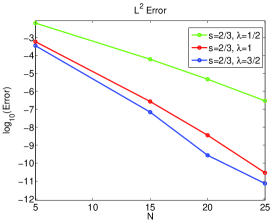
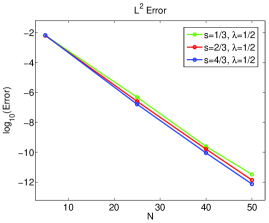
Figure 3.1. Convergence of the GLF approximation to (6.1) with $f(x)=e^{-x}\sin x\,.$

4. Generalized Laguerre functions: Type I (GLF-I)

In this section, we define and study a family of generalized Laguerre functions (GLFs) associated with the left-tempered fractional integral/derivative on the half line. It is seen from Definition 2.3 that the tempered fractional derivatives are introduced through the Fourier transform, having the alternative representations in Proposition 2.1. In what follows, the operators ${}_{0}{\rm I}_{x}^{\mu,\lambda},{{}_{0}}{\rm D}_{x}^{\mu,\lambda}$ on the half line should be understood as $0$ in place of $-\infty$ in (2.11) and (2.24)-(2.25).

4.1. Definition and properties

We first introduce the type of GJFs related to the “left-tempered” fractional integrals/derivatives.

Definition 4.1 (GLF-I).

For real $\alpha>-1$ and $\lambda>0,$ we define the GLF-I as

$${\mathcal{L}}^{(-\alpha,\lambda)}_{n}{(x)}:=x^{\alpha}e^{-\lambda x}\,{L}_{n}^{(\alpha)}(2\lambda x),\quad$$ (4.1)

for all $x\in\mathbb{R}^{+}$ and $n\in\mathbb{N}_{0}.$

One verifies readily from the orthogonality (2.49) and (4.1) that for $\alpha>-1$ and $\lambda>0,$

$$\int_{0}^{\infty}{\mathcal{L}}^{(-\alpha,\lambda)}_{n}{(x)}{\mathcal{L}}^{(-\alpha,\lambda)}_{m}{(x)}\,x^{-\alpha}dx=\gamma_{n}^{\alpha,\lambda}\delta_{nm},\;\;\;\gamma_{n}^{\alpha,\lambda}=\frac{\Gamma(n+\alpha+1)}{(2\lambda)^{\alpha+1}\,\Gamma(n+1)}.$$ (4.2)

We have the following important “tempered” fractional integral and derivative rules.

Lemma 4.1.

For $\mu,\lambda\in{\mathbb{R}}^{+},$ we have

$${}_{0}{\rm I}_{x}^{\mu,\lambda}{\mathcal{L}}^{(-\alpha,\lambda)}_{n}{(x)}=h^{\alpha,-\mu}_{n}{\mathcal{L}}^{(-\alpha-\mu,\lambda)}_{n}{(x)},\quad\alpha>-1,$$ (4.3)

$${{}_{0}}{\rm D}_{x}^{\mu,\lambda}{\mathcal{L}}^{(-\alpha,\lambda)}_{n}{(x)}=h^{\alpha,\mu}_{n}{\mathcal{L}}^{(\mu-\alpha,\lambda)}_{n}{(x)},\quad\alpha-\mu>-1,$$ (4.4)

and in addition, there holds

$${{}_{0}}{\rm D}_{x}^{\mu+k,\lambda}{\mathcal{L}}^{(-\mu,\lambda)}_{n}{(x)}=(-2\lambda)^{k}h^{\mu,\mu}_{n}e^{-\lambda x}\,L_{n-k}^{(k)}(2\lambda x),\quad n\geq k\in{\mathbb{N}}_{0}.$$ (4.5)

Proof.

We obtain from (2.11) and (2.24)-(2.25) (with replacing $-\infty$ by $0$) that

$${}_{0}{\rm I}_{x}^{\mu,\lambda}{\mathcal{L}}^{(-\alpha,\lambda)}_{n}{(x)}=e^{-\lambda x}{}_{0}{\rm I}_{x}^{\mu}\{e^{\lambda x}{\mathcal{L}}^{(-\alpha,\lambda)}_{n}{(x)}\}=e^{-\lambda x}{}_{0}{\rm I}_{x}^{\mu}\{x^{\alpha}L^{(\alpha)}_{n}(2\lambda x)\},$$

and

$${{}_{0}}{\rm D}_{x}^{\mu,\lambda}{\mathcal{L}}^{(-\alpha,\lambda)}_{n}{(x)}=e^{-\lambda x}{{}_{0}}{\rm D}_{x}^{\mu}\{e^{\lambda x}{\mathcal{L}}^{(-\alpha,\lambda)}_{n}{(x)}\}=e^{-\lambda x}{{}_{0}}{\rm D}_{x}^{\mu}\{x^{\alpha}L^{(\alpha)}_{n}(2\lambda x)\}.$$

Thus, from (B.11) and Lemma 2.2, we obtain (4.3)-(4.4).

Using (4.4) and the derivative relation (A.5) (with $\alpha=\mu$), we obtain

$${{}_{0}}{\rm D}_{x}^{\mu+k,\lambda}{\mathcal{L}}^{(-\mu,\lambda)}_{n}{(x)} ={{}_{0}}{\rm D}_{x}^{k,\lambda}{{}_{0}}{\rm D}_{x}^{\mu,\lambda}{\mathcal{L}}^{(-\mu,\lambda)}_{n}{(x)}=e^{-\lambda x}{}{\rm D}^{k}\big{\{}e^{\lambda x}h^{\mu,\mu}_{n}{\mathcal{L}}^{(0,\lambda)}_{n}{(x)}\big{\}}$$

$$=h^{\mu,\mu}_{n}\,e^{-\lambda x}{}{\rm D}^{k}\big{\{}L_{n}^{(0)}(2\lambda x)\big{\}}=(-2\lambda)^{k}h^{\mu,\mu}_{n}\,L_{n-k}^{(k)}(2\lambda x)\,e^{-\lambda x}.$$

This ends the proof. ∎

4.2. Approximation by GLF-I

Denote by $\mathcal{P}_{N}$ the set of all polynomials of degree at most $N$, and define the finite dimensional space

$$\mathcal{F}^{\alpha,\lambda}_{N}({\mathbb{R}}^{+}):=\big{\{}x^{\alpha}e^{-\lambda x}p(x)\,:\,p\in\mathcal{P}_{N}\big{\}},\quad N\in\mathbb{N}_{0}.$$ (4.6)

Define the $L_{\omega}^{2}({\mathbb{R}}^{+})$ with the inner product and norm:

$$(f,g)_{\omega}:=\int_{\Lambda}f\,\bar{g}\,\omega\,{\rm d}x,\quad\|f\|_{\omega}^{2}=(f,f)_{\omega},$$ (4.7)

where $\omega(x)\geq 0,~{}\forall x\in\mathbb{R}^{+}$, is a generic weight function and $\bar{g}$ is the conjugate of the function $g$. In particular, we omit $\omega$ when $\omega\equiv 1.$

To characterize the approximation errors, we define the non-uniformly weighted Sobolev space

$$A_{\alpha,\lambda}^{m}({\mathbb{R}}^{+}):=\Big{\{}u\in L^{2}_{\omega^{-\alpha}}({\mathbb{R}}^{+}):{{}_{0}}{\rm D}_{x}^{\alpha+k,\lambda}u\in L^{2}_{\omega^{k}}({\mathbb{R}}^{+}),\;k=0,\cdots,m\Big{\}},\quad m\in\mathbb{N}_{0},$$ (4.8)

equipped with the norm and semi-norm

$$\|u\|_{A_{\alpha,\lambda}^{m}}:=\Big{(}\|u\|^{2}_{\omega^{-\alpha}}+\sum_{k=0}^{m}\|{{}_{0}}{\rm D}_{x}^{\alpha+k,\lambda}u\|^{2}_{\omega^{k}}\Big{)}^{{1}/{2}},\quad|u|_{A_{\alpha,\lambda}^{m}}:=\|{{}_{0}}{\rm D}_{x}^{\alpha+m,\lambda}u\|_{\omega^{m}},$$ (4.9)

where the weight function $\omega^{a}(x)=x^{a}.$

Consider the orthogonal projection $\pi_{N}^{-\alpha,\lambda}:\,{L^{2}_{\omega^{-\alpha}}}({\mathbb{R}}^{+})\rightarrow\mathcal{F}^{\alpha,\lambda}_{N}({\mathbb{R}}^{+})$ defined by

$$(\pi_{N}^{-\alpha,\lambda}u-u,~{}\phi)_{\omega^{-\alpha}}=0,\quad\forall\phi\in\mathcal{F}^{\alpha,\lambda}_{N}({\mathbb{R}}^{+}),$$ (4.10)

where $\alpha>-1$. Then, by the orthogonality (4.2), $u$ and its $L^{2}$-orthogonal projection can be expanded as

$$u(x)=\sum_{n=0}^{\infty}~{}\hat{u}_{n}{\mathcal{L}}^{(-\alpha,\lambda)}_{n}{(x)},\quad(\pi_{N}^{-\alpha,\lambda}u)(x)=\sum_{n=0}^{N}~{}\hat{u}_{n}{\mathcal{L}}^{(-\alpha,\lambda)}_{n}{(x)},$$ (4.11)

where

$$\hat{u}_{n}=\big{(}u,~{}{\mathcal{L}}_{n}^{(-\alpha,\lambda)}\big{)}_{\omega^{-\alpha}}\big{/}\gamma^{\alpha,\lambda}_{n}.$$

Theorem 4.1.

For $\lambda>0$ and $\alpha>-1,$ we have that for any $u\in A^{m}_{\alpha,\lambda}(\mathbb{R}^{+})$ with $m\leq N+1$,

$$\|\pi_{N}^{-\alpha,\lambda}u-u\|_{\omega^{-\alpha}}\leq~{}c~{}(2\lambda N)^{-\frac{\alpha+m}{2}}~{}\|{{}_{0}}{\rm D}_{x}^{\alpha+m,\lambda}u\|_{\omega^{m}},$$ (4.12)

and for any $k\leq m,$

$$\big{\|}{{}_{0}}{\rm D}_{x}^{\alpha+k,\lambda}\big{(}\pi_{N}^{-\alpha,\lambda}u-u\big{)}\big{\|}_{\omega^{k}}\leq~{}c~{}({2\lambda}N)^{\frac{k-m}{2}}~{}\|{{}_{0}}{\rm D}_{x}^{\alpha+m,\lambda}u\|_{\omega^{m}},$$ (4.13)

where $c\approx 1$ for large $N.$

Proof.

By (4.11), we have

$$(u-\pi_{N}^{-\alpha,\lambda}u)(x)=\sum_{n=N+1}^{\infty}\,\hat{u}_{n}\,{\mathcal{L}}^{(-\alpha,\lambda)}_{n}{(x)}.$$

By the orthogonality (5.2) and (4.5),

$$\big{\|}{{}_{0}}{\rm D}_{x}^{\alpha+k,\lambda}{\mathcal{L}}^{(-\alpha,\lambda)}_{n}{}\big{\|}^{2}_{\omega^{k}}=(-2\lambda)^{2k}\,(h^{\alpha,\alpha}_{n})^{2}\int_{0}^{\infty}\big{(}L^{(k)}_{n-k}(2\lambda x)\big{)}^{2}\,e^{-2\lambda x}{\omega^{k}}(x){\rm d}x=(d_{n,k}^{\alpha,\lambda})^{2}\gamma_{n-k}^{k,\lambda},$$

where we denoted $d_{n,k}^{\alpha,\lambda}:=(2\lambda)^{k}\,h^{\alpha,\alpha}_{n}$ and used the fact:

$$\int_{0}^{\infty}L^{(m)}_{n-m}(2\lambda x)L^{(k)}_{n-k}(2\lambda x)\,e^{-2\lambda x}\omega^{k}dx=\frac{\gamma_{n-k}^{k}}{(2\lambda)^{k+1}}\delta_{km}=\gamma_{n-k}^{k,\lambda}\delta_{km},$$

Thus we can obtain

$$\|\pi_{N}^{-\alpha,\lambda}u-u\|^{2}_{\omega^{-\alpha}}=\sum_{n=N+1}^{\infty}(\hat{u}_{n})^{2}\gamma_{n}^{\alpha,\lambda},\quad\big{|}\pi_{N}^{-\alpha,\lambda}u-u\big{|}^{2}_{A^{k}_{\alpha,\lambda}}=\sum_{n=N+1}^{\infty}(\hat{u}_{n}d_{n,k}^{\alpha,\lambda})^{2}\gamma_{n-k}^{k,\lambda},$$

$$\big{|}u\big{|}^{2}_{A^{m}_{\alpha,\lambda}}=\sum_{n=m}^{\infty}(\hat{u}_{n}d_{n,m}^{\alpha,\lambda})^{2}\gamma_{n-m}^{m,\lambda}.$$

Then one verifies readily that

$$\|\pi_{N}^{-\alpha,\lambda}u-u\|^{2}_{\omega^{-\alpha}} \leq\frac{\gamma_{N+1}^{\alpha,\lambda}}{(d_{N+1,m}^{\alpha,\lambda})^{2}\gamma_{N+1-m}^{m,\lambda}}\big{|}u\big{|}^{2}_{A^{m}_{\alpha,\lambda}},$$

$$\quad\big{|}\pi_{N}^{-\alpha,\lambda}u-u\big{|}^{2}_{A^{k}_{\alpha,\lambda}} \leq\left(\frac{d_{N+1,k}^{\alpha,\lambda}}{d_{N+1,m}^{\alpha,\lambda}}\right)^{2}\frac{\gamma_{N+1-k}^{k,\lambda}}{\gamma_{N+1-m}^{m,\lambda}}\big{|}u\big{|}^{2}_{A^{m}_{\alpha,\lambda}}.$$

Recall the property of the Gamma function (see [1, (6.1.38)]):

$$\Gamma(x+1)=\sqrt{2\pi}x^{x+1/2}\exp\Big{(}-x+\frac{\theta}{12x}\Big{)},\quad\forall\,x>0,\;\;0<\theta<1.$$ (4.14)

One can then obtain that for any constants $a,b,$ and for $n\geq 1,$ $n+a>1$ and $n+b>1,$

$$\frac{\Gamma(n+a)}{\Gamma(n+b)}\leq\nu_{n}^{a,b}n^{a-b},$$ (4.15)

where

$$\nu_{n}^{a,b}=\exp\Big{(}\frac{a-b}{2(n+b-1)}+\frac{1}{12(n+a-1)}+\frac{(a-b)^{2}}{n}\Big{)}.$$ (4.16)

Therefore,

$$\frac{\gamma_{N+1}^{\alpha,\lambda}}{(d_{N+1,m}^{\alpha,\lambda})^{2}\gamma_{N+1-m}^{m,\lambda}} =\frac{\Gamma(N+2-m)}{(2\lambda)^{\alpha+m}\Gamma(N+2+\alpha)}\leq(2\lambda)^{-\alpha-m}\nu_{n}^{2-m,2+\alpha}N^{-\alpha-m},$$

$$\left(\frac{d_{N+1,k}^{\alpha,\lambda}}{d_{N+1,m}^{\alpha,\lambda}}\right)^{2}\frac{\gamma_{N+1-k}^{k,\lambda}}{\gamma_{N+1-m}^{m,\lambda}} =\frac{(2\lambda)^{k}\Gamma(N+2-m)}{(2\lambda)^{m}\Gamma(N+2-k)}<(2\lambda)^{k-m}\nu_{n}^{2-m,2-k}N^{k-m},$$

where $\nu_{n}^{2-m,2+\alpha}\approx 1$ and $\nu_{n}^{2-m,2-k}\approx 1$ for fixed $m$ and $n\geq N\gg 1$. Then (4.12)-(4.13) follow. ∎

4.3. A model problem and numerical results

In what follows, we consider the GLF-I approximation to a simple model tempered fractional equation of order $s\in[k-1,k)$ with $k\in\mathbb{N}:$

$${{}_{0}}{\rm D}_{x}^{s,\lambda}u(x)=f(x),\;\;x\in\mathbb{R}^{+},\;\;\lambda>0;\;\;u^{(j)}(0)=0,\quad j=0,1,\ldots,k-1,$$ (4.17)

where $f\in L^{2}(\mathbb{R}^{+})$ is a given function. Using the fractional derivative relation (B.9), one can find

$$u(x)={}_{0}{\rm I}_{x}^{s,\lambda}f(x)+\sum\limits_{i=1}^{k}c_{i}\,x^{s-i}e^{-\lambda x},$$

where $\{c_{i}\}$ can be determined by the conditions at $x=0.$ Indeed, we have all $c_{i}=0,$ and

$$u(x)={}_{0}{\rm I}_{x}^{s,\lambda}f(x)=\frac{e^{-\lambda x}}{\Gamma(s)}\int_{0}^{x}(x-\tau)^{s-1}e^{\lambda\tau}f(\tau){\rm d}\tau=\frac{x^{s}}{\Gamma(s)}\int_{0}^{1}(1-t)^{s-1}e^{-\lambda(1-t)x}f(xt){\rm d}t.$$ (4.18)

We see that if $f(x)$ is smooth, then $u(x)=x^{s}F(x),$ where $F(x)$ is smoother than $f(x).$ With this understanding, we construct the GLF-I Petrov-Galerkin approximation as: find $u_{N}\in\mathcal{F}^{s,\lambda}_{N}(\mathbb{R}^{+})$ (defined in (4.6)) such that

$$({{}_{0}}{\rm D}_{x}^{s,\lambda}u_{N},v_{N})=(f,v_{N}),\quad\forall\,v_{N}\in\mathcal{F}^{0,\lambda}_{N}(\mathbb{R}^{+}).$$ (4.19)

We expand $f$ and $u_{N}$ as

$$f(x)=\sum_{n=0}^{\infty}~{}\hat{f}_{n}{\mathcal{L}}^{(0,\lambda)}_{n}{(x)},~{}\quad u_{N}=\sum_{n=0}^{N}~{}\hat{u}_{n}{\mathcal{L}}^{(s,\lambda)}_{n}{(x)}.$$ (4.20)

Using the derivative relation (4.4), we find immediately that $\hat{u}_{n}=\frac{\gamma_{n}^{0,\lambda}}{h_{n}^{s,s}}\hat{f}_{n}$ for $n=0,1,\cdots,N$, which also implies ${{}_{0}}{\rm D}_{x}^{s,\lambda}u_{N}=\pi^{0,\lambda}_{N}f.$

Moreover, we can show that the numerical solution $u_{N}$ is precisely the orthogonal projection in the following sense:

$$(u_{N}-u\,,\,w_{N})_{\omega^{-s}}=0,\quad\forall\,w_{N}\in\mathcal{F}^{s,\lambda}_{N}(\mathbb{R}^{+}).$$ (4.21)

To this end, we first show

$$(u_{N}-u\,,\,{{}_{x}}{\rm D}_{\infty}^{s,\lambda}v_{N})=({{}_{0}}{\rm D}_{x}^{s,\lambda}u_{N}-{{}_{0}}{\rm D}_{x}^{s,\lambda}u,v_{N})=0,\quad\forall\,v_{N}\in\mathcal{F}^{0,\lambda}_{N}(\mathbb{R}^{+}).$$ (4.22)

Indeed, thanks to $u^{(j)}(0)=0$ for $j=0,\ldots,k-1$, we have

$${{}_{0}}{\rm D}_{x}^{s,\lambda}\{u_{N}-u\}=e^{-\lambda x}{{}_{0}}{\rm D}_{x}^{s}\{e^{\lambda x}(u_{N}-u)\}=e^{-\lambda x}{}_{0}{\rm I}_{x}^{k-s}{{}_{0}}{\rm D}_{x}^{k}\{e^{\lambda x}(u_{N}-u)\}.$$

Then,

$$\left({{}_{0}}{\rm D}_{x}^{s,\lambda}u_{N}-{{}_{0}}{\rm D}_{x}^{s,\lambda}u\,,\,v_{N}\right)=\left({}_{0}{\rm I}_{x}^{k-s}{{}_{0}}{\rm D}_{x}^{k}\{e^{\lambda x}(u_{N}-u)\},e^{-\lambda x}v_{N}\right)$$

$$\qquad=\left(e^{\lambda x}(u_{N}-u)\,,\,(-1)^{k}{\rm D}^{k}{}_{x}{\rm I}_{\infty}^{k-s,\lambda}v_{N}\right)=\left(u_{N}-u\,,\,{{}_{x}}{\rm D}_{\infty}^{s,\lambda}v_{N}\right),$$

so (6.13) is valid. In addition, thanks to Lemma 2.2 and (B.12), we have

$${{}_{x}}{\rm D}_{\infty}^{s,\lambda}{\mathcal{L}}^{(0,\lambda)}_{n}{(x)}=e^{\lambda x}{{}_{x}}{\rm D}_{\infty}^{s}\big{\{}e^{-2\lambda x}L^{(0)}_{n}(2\lambda{x})\big{\}}=(2\lambda)^{s}e^{-\lambda x}L^{(s)}_{n}(2\lambda{x})=(2\lambda)^{s}x^{-s}{\mathcal{L}}^{(-s,\lambda)}_{n}{(x)}.$$

Hence, (4.21) is valid.

Thanks to (4.21), we derive from Theorem 4.1 the following estimate where the convergence rate only depends on the regularity of the source term.

Theorem 4.2.

Let $u$ and $u_{N}$ be respectively the solutions of (6.1) and (6.12). Then for ${{}_{0}}{\rm D}_{x}^{m,\lambda}f\in L^{2}_{\omega^{m}}(I)$ with $m\in{\mathbb{N}}_{0},$ we have

$$\|u-u_{N}\|_{\omega^{-s}}\leq\,c\,(2\lambda N)^{-\frac{s+m}{2}}\,\|{{}_{0}}{\rm D}_{x}^{s+m,\lambda}u\|_{\omega^{m}}=c\,(2\lambda N)^{-\frac{s+m}{2}}\,\|{{}_{0}}{\rm D}_{x}^{m,\lambda}f\|_{\omega^{m}},$$ (4.23)

where $c\approx 1$ for large $N.$

We provide some numerical results to illustrate the convergence behaviour. We take $f(x)=e^{-x}\sin x$ and then evaluate the exact solution by (6.4). Note that as ${{}_{0}}{\rm D}_{x}^{m,\lambda}f=e^{-\lambda x}{}{\rm D}^{m}\{e^{\lambda x}f\}$, a direct calculation leads to

$$e^{-\lambda x}{}{\rm D}^{m}\{e^{\lambda x}f\}=e^{-\lambda x}\sum_{k=0}^{m}{m\choose{k}}\lambda^{m-k}e^{\lambda x}{}{\rm D}^{k}f=\sum_{k=0}^{m}{m\choose{k}}\lambda^{m-k}{}{\rm D}^{k}f.$$

We infer from (6.8) that the spectral accuracy can be achieved by the GLF-I approximation. Indeed, we observe from Figure 6.1 such a convergence behaviour.

Figure 4.1. Convergence of the GLF-I approximation to (6.1) with $f(x)=e^{-x}\sin x\,.$

4.4. Caputo-like tempered FDEs

Analogy to Caputo fractional derivative, the tempered Caputo-like fractional derivative can be defined by exchanging the order of the derivative operator and integral operator, we write the detail definition as follow: for any $\mu\in[k-1,k),~{}k\in\mathbb{N}$,

$${}_{0}^{C}{\rm D}_{x}^{\mu,\lambda}v:={}_{0}{\rm I}_{x}^{k-\mu,\lambda}{{}_{0}}{\rm D}_{x}^{k,\lambda}v=\frac{e^{-\lambda x}}{\Gamma(k-\mu)}\int_{0}^{x}(x-t)^{\mu-k+1}{}{\rm D}^{k}\{e^{\lambda t}v(t)\}{\rm d}t.$$ (4.24)

As stated in section 2, if we want the tempered Caputo-like fractional derivative ${}_{0}^{C}{\rm D}_{x}^{\mu,\lambda}v$ keeping the original definition of whole line tempered fractional derivative in which the zeros extension of function $v(x),~{}x\in\mathbb{R}^{+}$ satisfies $H(x)v(x)\in W^{k,2}_{\lambda}(\mathbb{R})$.

Akin to the analysis in section 2, for $\mu>1$, the zero initial value is necessary if we want to meet above condition. For any $\mu\in(0,1]$, we consider the below prototype problem as the typical for solving the tempered Caputo-like FDEs with non-zero initial value,

$${}_{0}^{C}{\rm D}_{x}^{\mu,\lambda}u(x)=f(x),\quad u(0)=u_{0},\quad x\in\mathbb{R}^{+}.$$ (4.25)

Via setting $v(x)=u(x)-u_{0}e^{-\lambda x}$, in view of (6.16), we can homogenize the problem as

$${}_{0}^{C}{\rm D}_{x}^{\mu,\lambda}v(x)=f(x),\quad v(0)=0,\quad x\in\mathbb{R}^{+}.$$ (4.26)

Furthermore, thanks to the relation between R-L fractional derivative and Caputo fractional derivative (B.10), the tempered Caputo-like FDE (6.17) is equivalent to a particular case in (6.11).

5. Generalized Laguerre functions of Type II

In this section, we introduce the second type GLFs related to the right tempered fractional integrals/derivatives, and study its spectral approximation property and applications to some model tempered fractional equations.

5.1. Definition and properties

Definition 5.1 (GLF-II).

For real $\alpha>-1$ and $\lambda>0,$ we define the GLF-II as

$$\breve{\mathcal{L}}^{(\alpha,\lambda)}_{n}{(x)}:={L}_{n}^{(\alpha)}(2\lambda x)~{}e^{-\lambda x},\quad x\in{\mathbb{R}}^{+},\;\;n\in{\mathbb{N}}_{0}.$$ (5.1)

In view of the orthogonality (2.49), we have that

$$\int_{0}^{\infty}\breve{\mathcal{L}}^{(\mu,\lambda)}_{n}{(x)}\breve{\mathcal{L}}^{(\mu,\lambda)}_{m}{(x)}\,x^{\mu}dx=\gamma_{n}^{\mu,\lambda}\delta_{nm},$$ (5.2)

where $\gamma_{n}^{\mu,\lambda}$ is the same to (4.2).

Moreover, by (B.11), (B.12) and Lemma 2.2, we have the following important formulas.

Lemma 5.1.

For $\lambda,\mu\in{\mathbb{R}}^{+},$ we have

$$\quad{}_{x}{\rm I}_{\infty}^{\mu,\lambda}\breve{\mathcal{L}}^{(\alpha,\lambda)}_{n}{(x)}=(2\lambda)^{-\mu}\breve{\mathcal{L}}^{(\alpha-\mu,\lambda)}_{n}{(x)},\quad\alpha>\mu-1,$$ (5.3)

$${{}_{x}}{\rm D}_{\infty}^{\mu,\lambda}\breve{\mathcal{L}}^{(\alpha,\lambda)}_{n}{(x)}=(2\lambda)^{\mu}\breve{\mathcal{L}}^{(\mu+\alpha,\lambda)}_{n}{(x)},\quad\alpha>-1,$$ (5.4)

Lemma 5.2.

Let $k\in\mathbb{N}$ and $\alpha>k-1$,

$${{}_{-\infty}}{\rm D}_{x}^{k,\lambda}\big{\{}x^{\alpha}\breve{\mathcal{L}}^{(\alpha,\lambda)}_{n}{(x)}\big{\}}=\frac{\Gamma(n+\alpha+1)}{\Gamma(n+\alpha-k+1)}~{}x^{\alpha-k}\breve{\mathcal{L}}^{(\alpha-k,\lambda)}_{n}{(x)},$$ (5.5)

$$\qquad{{}_{x}}{\rm D}_{\infty}^{k,\lambda}\big{\{}x^{\alpha}\breve{\mathcal{L}}^{(\alpha,\lambda)}_{n}{(x)}\big{\}}=(-1)^{k}\frac{\Gamma(n+k+1)}{\Gamma(n+1)}x^{\alpha-k}\breve{\mathcal{L}}^{(\alpha-k,\lambda)}_{n+k}{(x)}.\qquad$$ (5.6)

Proof.

From Lemma 2.2 and relation

$${{}_{-\infty}}{\rm D}_{x}^{k,\lambda}u=e^{-\lambda x}{}{\rm D}^{k}\big{\{}e^{\lambda x}u\big{\}},\quad{{}_{x}}{\rm D}_{\infty}^{k,\lambda}u=e^{\lambda x}(-1)^{k}{}{\rm D}^{k}\big{\{}e^{-\lambda x}u\big{\}},$$ (5.7)

we obtain

$${{}_{-\infty}}{\rm D}_{x}^{k,\lambda} \big{\{}x^{\alpha}\breve{\mathcal{L}}^{(\alpha,\lambda)}_{n}{(x)}\big{\}}=e^{-\lambda x}{}{\rm D}^{k}\big{\{}(2\lambda)^{-\alpha}(2\lambda x)^{\alpha}L^{(\alpha)}_{n}(2\lambda x)\big{\}}$$

$$\overset{\eqref{lagupolyderi}}{=} \frac{\Gamma(n+1+\alpha)}{\Gamma(n+\alpha-k+1)}x^{\alpha-k}L^{(\alpha-k)}_{n}(2\lambda x)e^{-\lambda x}=\frac{\Gamma(n+1+\alpha)}{\Gamma(n+\alpha-k+1)}~{}x^{\alpha-k}\breve{\mathcal{L}}^{(\alpha-k,\lambda)}_{n}{(x)},$$

and

$${{}_{x}}{\rm D}_{\infty}^{k,\lambda}\big{\{}x^{\alpha}\breve{\mathcal{L}}^{(\alpha,\lambda)}_{n}{(x)}\big{\}}= e^{\lambda x}(-1)^{k}{}{\rm D}^{k}\big{\{}(2\lambda)^{-\alpha}(2\lambda x)^{\alpha}L^{(\alpha)}_{n}(2\lambda x)e^{-2\lambda x}\big{\}}$$ (5.8)

$$\overset{\eqref{lagufunderi}}{=} (-1)^{k}\frac{\Gamma(n+k+1)}{\Gamma(n+1)}x^{\alpha-k}L^{(\alpha-k)}_{n+k}(2\lambda x)e^{-\lambda x}$$

$$= (-1)^{k}\frac{\Gamma(n+k+1)}{\Gamma(n+1)}~{}x^{\alpha-k}\breve{\mathcal{L}}^{(\alpha-k,\lambda)}_{n}{(x)}.$$

This ends the proof. ∎

5.2. Approximation by GLF-II

Introduce the non-uniformly weighted Sobolev space:

$$B_{\beta,\lambda}^{r}(\mathbb{R}^{+}):=\Big{\{}u\in L^{2}_{\omega^{\beta}}({\mathbb{R}}^{+}):{{}_{x}}{\rm D}_{\infty}^{s,\lambda}u\in L^{2}_{\omega^{\beta+s}}({\mathbb{R}}^{+}),\;0\leq s\leq r\Big{\}},\quad r\in\mathbb{R}^{+}_{0},$$ (5.9)

endowed with norm and semi-norm

$$\|u\|_{B_{\beta,\lambda}^{r}}:=\Big{(}\|u\|^{2}_{\omega^{\beta}}+|u|^{2}_{B_{\beta,\lambda}^{r}}\Big{)}^{{1}/{2}},\quad|u|_{B_{\beta}^{r}}:=\|{{}_{x}}{\rm D}_{\infty}^{\beta+r,\lambda}u\|_{\omega^{\beta+r}}.$$ (5.10)

Consider the orthogonal projection $\Pi_{N}^{\beta,\lambda}:~{}{L^{2}_{\omega^{\beta}}}({\mathbb{R}}^{+})\rightarrow\mathcal{F}^{\lambda}_{N}({\mathbb{R}}^{+}),$ defined by

$$\big{(}\Pi_{N}^{\beta,\lambda}u-u,~{}\phi\big{)}_{\omega^{\beta}}=0,\quad\forall\phi\in\mathcal{F}^{\lambda}_{N}({\mathbb{R}}^{+}),\quad\beta>-1,$$ (5.11)

where

$$\mathcal{F}^{\lambda}_{N}({\mathbb{R}}^{+}):=\mathcal{F}^{0,\lambda}_{N}(\mathbb{R}^{+})=\big{\{}p(x)e^{-\lambda x}:~{}p\in\mathcal{P}_{N}\big{\}},\quad N\in\mathbb{N},\;\;\lambda>0.$$ (5.12)

Theorem 5.1.

For $\lambda,r>0$, $\beta>-1,$ and for $u\in B^{r}_{\beta,\lambda}({\mathbb{R}}^{+})$ with $0\leq s\leq r\leq N,$ we have

$$\big{\|}{{}_{x}}{\rm D}_{\infty}^{s,\lambda}\big{\{}\Pi_{N}^{\beta,\lambda}u-u\big{\}}\big{\|}_{\omega^{\beta+s}}\leq~{}c~{}({2\lambda}{N})^{\frac{s-r}{2}}~{}\|{{}_{x}}{\rm D}_{\infty}^{r,\lambda}u\|_{\omega^{\beta+r}},$$ (5.13)

where $c\approx 1$ for large $N.$

Proof.

Note that by definition,

$$u-\Pi_{N}^{\beta,\lambda}u=\sum_{n=N+1}^{\infty}~{}\hat{u}_{n}\breve{\mathcal{L}}_{n}^{(\beta,\lambda)}(x),\quad\hat{u}_{n}=\big{(}u,~{}\breve{\mathcal{L}}_{n}^{(\beta,\lambda)}\big{)}_{\omega^{\beta}}\big{/}\gamma^{\beta,\lambda}_{n}.$$

Then by (5.4), and the orthgogonality,

$$\|{{}_{x}}{\rm D}_{\infty}^{s,\lambda}\breve{\mathcal{L}}^{(\beta,\lambda)}_{n}{}\|^{2}_{\omega^{\beta+s}}=\|\breve{\mathcal{L}}^{(\beta+s,\lambda)}_{n}{}\|^{2}_{\omega^{\beta+s}}=\gamma_{n}^{\beta+s,\lambda},$$

we can derive

$$\big{|}\Pi_{N}^{\beta,\lambda}u-u\big{|}^{2}_{B^{s}_{\beta,\lambda}} =\|\sum_{n=N+1}^{\infty}\hat{u}_{n}(2\lambda)^{s}\breve{\mathcal{L}}^{(\beta+s,\lambda)}_{n}{}\|^{2}_{\omega^{\beta+s}}=\sum_{n=N+1}^{\infty}(\hat{u}_{n})^{2}(2\lambda)^{2s}\gamma_{n}^{\beta+s,\lambda},$$

$$\big{|}u\big{|}^{2}_{B^{r}_{\beta+r,\lambda}} =\|\sum_{n=0}^{\infty}\hat{u}_{n}(2\lambda)^{r}\breve{\mathcal{L}}^{(n,\lambda)}_{\beta+r}{}\|^{2}_{\omega^{\beta+r}}=\sum_{n=0}^{\infty}(\hat{u}_{n})^{2}(2\lambda)^{2r}\gamma_{n}^{\beta+r,\lambda}.$$

Then,

$$\big{|}\Pi_{N}^{\beta,\lambda}u-u\big{|}^{2}_{B^{s}_{\beta,\lambda}} =\sum_{n=N+1}^{\infty}(\hat{u}_{n})^{2}\gamma_{n}^{\beta+s,\lambda}\leq(2\lambda)^{2s-2r}\frac{\gamma_{N+1}^{\beta+s,\lambda}}{\gamma_{N+1}^{\beta+r,\lambda}}\sum_{n=N+1}^{\infty}(\hat{u}_{n})^{2}\gamma_{n}^{\beta+r,\lambda},$$

where by (4.15)-(4.16), we obtain

$$\dfrac{\gamma_{N+1}^{\beta+s,\lambda}}{\gamma_{N+1}^{\beta+r,\lambda}}=\dfrac{(2\lambda)^{r}\Gamma(N+\beta+s+2)}{(2\lambda)^{s}\Gamma(N+\beta+r+2)}\leq c({2\lambda})^{r-s}N^{s-r}.$$

Consequently, we have

$$\|{{}_{x}}{\rm D}_{\infty}^{s,\lambda}\big{\{}\Pi_{N}^{\beta,\lambda}u-u\big{\}}\|_{\omega^{\beta+s}}\leq~{}c\,({2\lambda}N)^{\frac{s-r}{2}}\,|u|_{B^{r}_{\beta,\lambda}}.$$

This ends the proof. ∎

Remark 5.1.

GLF-I and GLF-II are respectively utilized to derive the Theorem 4.1 and the Theorem 5.1. They are different

The GLF-II was tailored for the right tempered derivative, different from the extended left tempered derivative ${{}_{0}}{\rm D}_{x}^{\mu,\lambda}$, there is no singular point at $x=0$ Furthermore, set $m=0,~{}\beta=0$ in $A^{m}_{\alpha,\lambda}$ and $B^{r}_{\beta,\lambda}$ respectively, we have the following more accurate estimate than Theorem 4.1.

Corollary 5.2.

Let $\lambda,r>0$, $\alpha>-1$. If $u\in A^{0}_{\alpha,\lambda}\cap B^{r}_{0,\lambda}$, then

$$\|\,\pi_{N}^{-\alpha,\lambda}u-u\|_{\omega^{-\alpha}}\leq~{}c~{}({2\lambda}{N})^{-\frac{\alpha+r}{2}}~{}\|{{}_{x}}{\rm D}_{\infty}^{r,\lambda}{{}_{0}}{\rm D}_{x}^{\alpha,\lambda}u\|_{\omega^{r}}.$$ (5.14)

In addition, for $0\leq s\leq r$,

$$\|{{}_{x}}{\rm D}_{\infty}^{s,\lambda}{{}_{0}}{\rm D}_{x}^{\alpha,\lambda}\big{\{}\pi_{N}^{-\alpha,\lambda}u-u\big{\}}\|_{\omega^{s}}\leq~{}c~{}({2\lambda}N)^{\frac{s-r}{2}}~{}\|{{}_{x}}{\rm D}_{\infty}^{r,\lambda}{{}_{0}}{\rm D}_{x}^{\alpha,\lambda}u\|_{\omega^{r}}.$$ (5.15)

Proof.

By the direct calculation, we can show that ${{}_{0}}{\rm D}_{x}^{\alpha,\lambda}\pi_{N}^{-\alpha,\lambda}u=\Pi^{0,\lambda}_{N}u$. Then Corollary 5.2 is the straightforward conclusion of Theorem 5.1. ∎

5.3. A model problem and numerical results

We consider the right tempered fractional equation:

$${{}_{x}}{\rm D}_{\infty}^{s,\lambda}u(x)=f(x),\quad x\in\mathbb{R}^{+},\;\;\lambda>0;\;\;\lim_{x\rightarrow\infty}u^{(j)}(x)=0,\quad j=0,1,\ldots,k-1,$$ (5.16)

where $s\in[k-1,k)$ with $k\in\mathbb{N}$.

Since $\lim\limits_{x\rightarrow\infty}e^{-\lambda x}u(x)=0$, the solution can be derived from

$${}_{x}{\rm I}_{\infty}^{s,\lambda}f={}_{x}{\rm I}_{\infty}^{s,\lambda}\,{{}_{x}}{\rm D}_{\infty}^{s,\lambda}u=e^{\lambda x}{}_{x}{\rm I}_{\infty}^{s}\,{{}_{x}}{\rm D}_{\infty}^{s}\big{\{}e^{-\lambda x}u\big{\}}=u.$$ (5.17)

Assume that $f\in L^{2}_{\omega^{\alpha}}(\mathbb{R}^{+})$ with $\alpha>s-1$. Then we have from (5.2) that

$$f(x)=\sum\limits_{n=0}^{\infty}\hat{f}_{n}\breve{\mathcal{L}}^{(\alpha,\lambda)}_{n}{(x)},\quad\|f\|^{2}_{\omega^{\alpha}}=\sum\limits_{n=0}^{\infty}|\hat{f}_{n}|^{2}\,\gamma^{\alpha,\lambda}_{n}.$$

Thanks to (5.3), we find that for any $0\leq\nu\leq s$,

$${{}_{x}}{\rm D}_{\infty}^{\nu,\lambda}u(x)={}_{x}{\rm I}_{\infty}^{s-\nu,\lambda}f(x)=\sum\limits_{n=0}^{\infty}\hat{f}_{n}\,{}_{x}{\rm I}_{\infty}^{s-\nu,\lambda}\breve{\mathcal{L}}^{(\alpha,\lambda)}_{n}{(x)}=\sum\limits_{n=0}^{\infty}(2\lambda)^{\nu-s}\hat{f}_{n}\,\breve{\mathcal{L}}^{(\alpha-s+\nu,\lambda)}_{n}{(x)}.\\$$ (5.18)

Then,

$$\|{{}_{x}}{\rm D}_{\infty}^{\nu,\lambda}u\|_{\omega^{\alpha-s+\nu}}^{2} =\sum\limits_{n=0}^{\infty}|(2\lambda)^{\nu-s}\hat{f}_{n}|^{2}\,\gamma^{\alpha-s+\nu,\lambda}_{n}=\sum\limits_{n=0}^{\infty}\frac{\Gamma(n+\alpha-s+\nu+1)}{(2\lambda)^{s-\nu+\alpha+1}\Gamma(n+1)}|\hat{f}_{n}|^{2}$$ (5.19)

$$\leq\frac{\Gamma(\alpha-s+\nu+1)}{(2\lambda)^{s-\nu}\Gamma(\alpha+1)}\|f\|^{2}_{\omega^{\alpha}}<\infty,$$

which implies that ${{}_{x}}{\rm D}_{\infty}^{\nu,\lambda}u\in L_{\omega^{\alpha-s+\nu}}^{2}(\mathbb{R}^{+}),~{}0\leq\nu\leq s$, namely, $u\in B^{s}_{\alpha-s,\lambda}(\mathbb{R}^{+})$.

The GLF-II Galerkin method for (6.2) is to find $u_{N}\in\mathcal{F}^{\lambda}_{N}(\mathbb{R}^{+})$ such that

$$({{}_{x}}{\rm D}_{\infty}^{s,\lambda}u_{N},v_{N})=(f,v_{N}),\quad\forall v_{N}\in\mathcal{F}^{\lambda}_{N}(\mathbb{R}^{+}).$$ (5.20)

Furthermore, thanks to the orthogonality (5.2), we deduce that the solution of (6.14) is given by

$$u_{N}=\sum\limits_{n=0}^{N}(2\lambda)^{-s}\hat{f}_{n}\breve{\mathcal{L}}^{(\alpha-s,\lambda)}_{n}{(x)}$$

which is exactly the orthogonal projection from $L^{2}_{\omega^{\alpha-s}}(\mathbb{R}^{+})$ to $\mathcal{F}^{\lambda}_{N}(\mathbb{R}^{+})$ (see (5.12)). Thus, the following estimate is an immediate consequence of Theorem 5.1.

Theorem 5.2.

Let $u$ and $u_{N}$ be the solutions of (6.2) and (6.14), respectively. If $f\in L^{2}_{\omega^{\alpha}}(\mathbb{R}^{+})$ and ${{}_{x}}{\rm D}_{\infty}^{r-s,\lambda}f\in L^{2}_{\omega^{\alpha-s+r}}(I)$ with $\alpha>s-1$, then we have

$$\|u-u_{N}\|_{\omega^{\alpha-s}}\leq c\,({2\lambda}{N})^{-\frac{r}{2}}\|{{}_{x}}{\rm D}_{\infty}^{r,\lambda}u\|_{\omega^{\alpha-s+r}}=c\,({2\lambda}{N})^{-\frac{r}{2}}\|{{}_{x}}{\rm D}_{\infty}^{r-s,\lambda}f\|_{\omega^{\alpha-s+r}},$$ (5.21)

where $c\approx 1$ for large $N.$

We depict in Figure 6.2 the convergence of the GLF-II approximation, from which we observe exponential decay of the errors for two examples with various order $s.$ Different from the left tempered case, the solution has no singularity at $x=0,$ so the GLF-II in (5.1) is expected to provide an accurate approximation if the solution decays rapidly.

Figure 5.1. Convergence of the GLF-II approximation to (6.2). Left: $u(x)=e^{-x}$ and $f(x)=(1+\lambda)^{s}\,e^{-x}.$ Right: $f(x)=e^{-x}\cos x$.

6. Applications to tempered FDEs on the half line

Before we pay our attentions to the tempered fractional diffusion equation, it’s necessary to figure out the role of the tempered derivative in a specific problem. In this section, we step on two classes of prototype tempered fractional derivative problems: the extended left tempered FDE

$${{}_{0}}{\rm D}_{x}^{s,\lambda}u(x)=f(x),\quad x\in\mathbb{R}^{+},$$ (6.1)

and right tempered FDE

$${{}_{x}}{\rm D}_{\infty}^{s,\lambda}u(x)=f(x),\quad x\in\mathbb{R}^{+},$$ (6.2)

where $s\in[k-1,k)$ with $k\in\mathbb{N}$. Moreover, akin to the Caputo fractional derivative, we briefly discussed Caputo-like tempered FDE in the last part of this section.

6.1. The extended left tempered FDEs

In order to design the efficient spectral method approximating the extended left tempered FDEs, it’s beneficial to investigate the solution’s regularity. Via the fractional derivative relation (B.9), it’s easy to derive the exact solution of the problem (6.1),

$$u(x)={}_{0}{\rm I}_{x}^{s,\lambda}f(x)+\sum\limits_{i=1}^{k}c_{i}\,x^{s-i}e^{-\lambda x},$$

where $c_{i},~{}i=1,2,\ldots,k$ are some constants.

As mentioned in the previous part, condition (2.40) is a necessity for the extended tempered fractional derivative ${{}_{0}}{\rm D}_{x}^{s,\lambda}u(x)$, then the solution reduces to

$$u(x)={}_{0}{\rm I}_{x}^{s,\lambda}f(x)+c_{1}\,x^{s-1}e^{-\lambda x}.$$ (6.3)

Moreover, if $f(x)$ is analytic in the vicinity of the zero, then

$${}_{0}{\rm I}_{x}^{s,\lambda}f(x)=\frac{e^{-\lambda x}}{\Gamma(s)}\int_{0}^{x}(x-\tau)^{s-1}e^{\lambda\tau}f(\tau)d\tau=\frac{x^{s}}{\Gamma(s)}\int_{0}^{1}(1-t)^{s-1}e^{\lambda(t-1)x}f(xt)dt$$ (6.4)

implies that $u(x)$ has the singularity $x^{s}+c_{x}x^{s-1}$ near zero.

Now, we consider below homogeneous initial value problem

$${{}_{0}}{\rm D}_{x}^{s,\lambda}u(x)=f(x),\quad D^{j}u(0)=0,\quad j=0,1,\ldots,k-1.$$ (6.5)

As zero initial value determine that the solution’s singularity is $x^{s}$, the related GLF Petrov-Galerkin method is to find $u_{N}\in\mathcal{F}^{s,\lambda}_{N}(\mathbb{R}^{+})$ (defined in (4.6)) such that

$$({{}_{0}}{\rm D}_{x}^{s,\lambda}u_{N},v_{N})=(f,v_{N}),\quad\forall v_{N}\in\mathcal{F}^{0,\lambda}_{N}(\mathbb{R}^{+}).$$ (6.6)

Writing

$$f=\sum_{n=0}^{\infty}~{}\hat{f}_{n}{\mathcal{L}}^{(0,\lambda)}_{n}{(x)},~{}\quad\pi^{0,\lambda}_{N}f=\sum_{n=0}^{N}~{}\hat{f}_{n}{\mathcal{L}}^{(0,\lambda)}_{n}{(x)},$$

we derive from (6.12) that

$$({{}_{0}}{\rm D}_{x}^{s,\lambda}u_{N}-f,v_{N})=({{}_{0}}{\rm D}_{x}^{s,\lambda}u_{N}-{{}_{0}}{\rm D}_{x}^{s,\lambda}u,v_{N})=0,\quad\forall~{}v_{N}\in\mathcal{F}^{0,\lambda}_{N}(\mathbb{R}^{+}),$$

namely,

$${{}_{0}}{\rm D}_{x}^{s,\lambda}u_{N}=\pi^{0,\lambda}_{N}f,\quad\|{{}_{0}}{\rm D}_{x}^{s,\lambda}(u_{N}-u)\|=\|\pi^{0,\lambda}_{N}f-f\|.$$

Moreover, we can prove our numerical solution $u_{N}$ of the scheme (6.12) is precisely the projection $\pi^{-s,\lambda}_{N}u$. In fact, as $u^{j}(0)=0,~{}j=0,\ldots,k-1$, we first show that

$$(u_{N}-u\,,\,{{}_{x}}{\rm D}_{\infty}^{s,\lambda}v_{N})=({{}_{0}}{\rm D}_{x}^{s,\lambda}u_{N}-{{}_{0}}{\rm D}_{x}^{s,\lambda}u,v_{N})=0,\quad\forall~{}v_{N}\in\mathcal{F}^{0,\lambda}_{N}(\mathbb{R}^{+}).$$ (6.7)

Indeed, due to $u^{j}(0)=0,~{}j=0,\ldots,k-1$, we can derive from (B.10) that

$${{}_{0}}{\rm D}_{x}^{s,\lambda}(u_{N}-u)=e^{-\lambda x}{{}_{0}}{\rm D}_{x}^{s}\{e^{\lambda x}(u_{N}-u)\}=e^{-\lambda x}{}_{0}{\rm I}_{x}^{k-s}{{}_{0}}{\rm D}_{x}^{k}\{e^{\lambda x}(u_{N}-u)\}.$$

Then,

$$\left({{}_{0}}{\rm D}_{x}^{s,\lambda}u_{N}-{{}_{0}}{\rm D}_{x}^{s,\lambda}u\,,\,v_{N}\right) =\left({}_{0}{\rm I}_{x}^{k-s}{{}_{0}}{\rm D}_{x}^{k}\{e^{\lambda x}(u_{N}-u)\},e^{-\lambda x}v_{N}\right)$$

$$~{}\overset{\eqref{Int-exchange}}{=} \left(D^{k}\{e^{\lambda x}(u_{N}-u)\}u_{N}-u\,,\,{}_{x}{\rm I}_{\infty}^{k-s,\lambda}v_{N}\right)$$

$$= \left(e^{\lambda x}(u_{N}-u)\,,\,(-1)^{k}D^{k}{}_{x}{\rm I}_{\infty}^{k-s,\lambda}v_{N}\right)$$

$$= \left(u_{N}-u\,,\,{{}_{x}}{\rm D}_{\infty}^{s,\lambda}v_{N}\right).$$

namely, (6.13) is valid. In additional, as

$${{}_{x}}{\rm D}_{\infty}^{s,\lambda}{\mathcal{L}}^{(0,\lambda)}_{n}{(x)}={{}_{x}}{\rm D}_{\infty}^{s,\lambda}\breve{\mathcal{L}}^{(0,\lambda)}_{n}{x}=\breve{\mathcal{L}}^{(s,\lambda)}_{n}{(x)}=x^{-s}{\mathcal{L}}^{(-s,\lambda)}_{n}{(x)},$$

leads to

$$(u_{N}-u\,,\,w_{N})_{\omega^{-s}}=0,\quad\forall~{}w_{N}\in\mathcal{F}^{s,\lambda}_{N}(\mathbb{R}^{+}).$$

The numerical solution is equivalent to projection $\pi_{N}^{-s,\lambda}u$ and has the following estimate,

Theorem 6.1.

Let $u$ and $u_{N}$ be respectively the solutions of (6.11) and (6.12). if $u\in A^{m}_{s,\lambda}(\mathbb{R}^{+})$, then

$$\|u-u_{N}\|_{\omega^{-s}}\leq~{}c~{}(2\lambda N)^{-\frac{s+m}{2}}~{}\|{{}_{0}}{\rm D}_{x}^{s+m,\lambda}u\|_{\omega^{m}}.$$ (6.8)

Remark 6.1.

tempered fractional differential equation is an extension of differential equation. For example, as

$${{}_{0}}{\rm D}_{x}^{1,\lambda}u(x)=e^{-\lambda x}D(e^{\lambda x}u(x))=u^{\prime}(x)+\lambda u(x),$$

and the inhomogeneous initial condition can be homogenized by subtracting $u_{0}e^{-\lambda x}$ from $u(x)$, the prototype problem (6.1) is equivalent to below ordinary differential equation

$$u^{\prime}(x)+\lambda u(x)=f(x),\quad u(0)=0.$$

6.2. The extended left tempered FDEs

In order to design the efficient spectral method approximating the extended left tempered FDEs, it’s beneficial to investigate the solution’s regularity. Via the fractional derivative relation (B.9), it’s easy to derive the exact solution of the problem (6.1),

$$u(x)={}_{0}{\rm I}_{x}^{s,\lambda}f(x)+\sum\limits_{i=1}^{k}c_{i}\,x^{s-i}e^{-\lambda x},$$

where $c_{i},~{}i=1,2,\ldots,k$ are some constants.

As mentioned in the previous part, condition (2.40) is a necessity for the extended tempered fractional derivative ${{}_{0}}{\rm D}_{x}^{s,\lambda}u(x)$, then the solution reduces to

$$u(x)={}_{0}{\rm I}_{x}^{s,\lambda}f(x)+c_{1}\,x^{s-1}e^{-\lambda x}.$$ (6.9)

Furthermore, assume $f\in C(\mathbb{R^{+}})\cap L^{2}(\mathbb{R^{+}})$,

$$\lim_{x\rightarrow 0}{}_{0}{\rm I}_{x}^{s,\lambda}f(x) =\lim_{x\rightarrow 0}e^{-\lambda x}\int_{0}^{x}(x-\tau)^{s-1}e^{\lambda\tau}f(\tau)d\tau$$

$$\leq\|f\|_{\infty}~{}\lim_{x\rightarrow 0}~{}e^{-\lambda x}\int_{0}^{x}(x-\tau)^{s-1}e^{\lambda\tau}d\tau$$

$$=\|f\|_{\infty}~{}\lim_{x\rightarrow 0}~{}x^{s}\int_{0}^{1}(1-t)^{s-1}e^{\lambda(t-1)x}dt=0.$$

Hence, in order to ensure that $D^{k-1}u(0)$ or ${{}_{0}}{\rm D}_{x}^{s-1,\lambda}u(0)$ is finite, we derive from (6.9) that there are only two suitable sets of initial conditions:

$$\textbf{Type I}:{} D^{j}u(0)=0,\quad j=0,1,\ldots,k-1;$$ (6.10)

$$\textbf{Type II}:{} D^{j}u(0)=0,\quad j=0,1,\ldots,k-2,\quad{{}_{0}}{\rm D}_{x}^{s-1,\lambda}u(0)=u_{0}.$$

Now, we concentrate on the tempered fractional differential equation with the two types of initial conditions in (6.10).

6.2.1. Type I

Let $s\in[k-1,k)$ and $f\in L^{2}(\Lambda)\cap C(\Lambda)$. Consider the problem

$${{}_{0}}{\rm D}_{x}^{s,\lambda}u(x)=f(x),\quad D^{j}u(0)=0,\quad j=0,1,\ldots,k-1.$$ (6.11)

The GLF Petrov-Galerkin method is to find $u_{N}\in\mathcal{F}^{s,\lambda}_{N}(\mathbb{R}^{+})$ (cf. (4.6)) such that

$$({{}_{0}}{\rm D}_{x}^{s,\lambda}u_{N},v_{N})=(f,v_{N}),\quad\forall v_{N}\in\mathcal{F}^{0,\lambda}_{N}(\mathbb{R}^{+}).$$ (6.12)

Writing

$$f=\sum_{n=0}^{\infty}~{}\hat{f}_{n}{\mathcal{L}}^{(0,\lambda)}_{n}{(x)},~{}\quad\pi^{0,\lambda}_{N}f=\sum_{n=0}^{N}~{}\hat{f}_{n}{\mathcal{L}}^{(0,\lambda)}_{n}{(x)},$$

we derive from (6.12) that

$$({{}_{0}}{\rm D}_{x}^{s,\lambda}u_{N}-f,v_{N})=({{}_{0}}{\rm D}_{x}^{s,\lambda}u_{N}-{{}_{0}}{\rm D}_{x}^{s,\lambda}u,v_{N})=0,\quad\forall~{}v_{N}\in\mathcal{F}^{0,\lambda}_{N}(\mathbb{R}^{+}),$$

namely,

$${{}_{0}}{\rm D}_{x}^{s,\lambda}u_{N}=\pi^{0,\lambda}_{N}f,\quad\|{{}_{0}}{\rm D}_{x}^{s,\lambda}(u_{N}-u)\|=\|\pi^{0,\lambda}_{N}f-f\|.$$

Moreover, we can prove our numerical solution $u_{N}$ of the scheme (6.12) is precisely the projection $\pi^{-s,\lambda}_{N}u$. In fact, as $u^{j}(0)=0,~{}j=0,\ldots,k-1$, we first show that

$$(u_{N}-u\,,\,{{}_{x}}{\rm D}_{\infty}^{s,\lambda}v_{N})=({{}_{0}}{\rm D}_{x}^{s,\lambda}u_{N}-{{}_{0}}{\rm D}_{x}^{s,\lambda}u,v_{N})=0,\quad\forall~{}v_{N}\in\mathcal{F}^{0,\lambda}_{N}(\mathbb{R}^{+}).$$ (6.13)

Indeed, due to $u^{j}(0)=0,~{}j=0,\ldots,k-1$, we can derive from (B.10) that

$${{}_{0}}{\rm D}_{x}^{s,\lambda}(u_{N}-u)=e^{-\lambda x}{{}_{0}}{\rm D}_{x}^{s}\{e^{\lambda x}(u_{N}-u)\}=e^{-\lambda x}{}_{0}{\rm I}_{x}^{k-s}{{}_{0}}{\rm D}_{x}^{k}\{e^{\lambda x}(u_{N}-u)\}.$$

Then,

$$\left({{}_{0}}{\rm D}_{x}^{s,\lambda}u_{N}-{{}_{0}}{\rm D}_{x}^{s,\lambda}u\,,\,v_{N}\right) =\left({}_{0}{\rm I}_{x}^{k-s}{{}_{0}}{\rm D}_{x}^{k}\{e^{\lambda x}(u_{N}-u)\},e^{-\lambda x}v_{N}\right)$$

$$~{}\overset{\eqref{Int-exchange}}{=} \left(D^{k}\{e^{\lambda x}(u_{N}-u)\}u_{N}-u\,,\,{}_{x}{\rm I}_{\infty}^{k-s,\lambda}v_{N}\right)$$

$$= \left(e^{\lambda x}(u_{N}-u)\,,\,(-1)^{k}D^{k}{}_{x}{\rm I}_{\infty}^{k-s,\lambda}v_{N}\right)$$

$$= \left(u_{N}-u\,,\,{{}_{x}}{\rm D}_{\infty}^{s,\lambda}v_{N}\right).$$

namely, (6.13) is valid.

Due to

$${{}_{x}}{\rm D}_{\infty}^{s,\lambda}{\mathcal{L}}^{(0,\lambda)}_{n}{(x)}={{}_{x}}{\rm D}_{\infty}^{s,\lambda}\breve{\mathcal{L}}^{(0,\lambda)}_{n}{x}=\breve{\mathcal{L}}^{(s,\lambda)}_{n}{(x)}=x^{-s}{\mathcal{L}}^{(-s,\lambda)}_{n}{(x)},$$

the above is equivalent to

$$(u_{N}-u\,,\,w_{N})_{\omega^{-s}}=0,\quad\forall~{}w_{N}\in\mathcal{F}^{s,\lambda}_{N}(\mathbb{R}^{+}).$$

Remark 6.2.

tempered fractional differential equation is an extension of differential equation. For example, as

$${{}_{0}}{\rm D}_{x}^{1,\lambda}u(x)=e^{-\lambda x}D(e^{\lambda x}u(x))=u^{\prime}(x)+\lambda u(x),$$

and the inhomogeneous initial condition can be homogenized by subtracting $u_{0}e^{-\lambda x}$ from $u(x)$, the prototype problem (6.1) is equivalent to below ordinary differential equation

$$u^{\prime}(x)+\lambda u(x)=f(x),\quad u(0)=0.$$

An numerical test with smooth data $f(x)=\sin xe^{-x}$ in Figure 6.1 validates the error analysis.

Figure 6.1. Resource term: $f(x)=\sin xe^{-x}$

6.3. Right tempered FDEs

Different from the extended tempered derivative ${{}_{0}}{\rm D}_{x}^{s,\lambda}$, the right tempered fractional derivative ${{}_{x}}{\rm D}_{\infty}^{s,\lambda}$ does not require homogeneous conditions at $x=0$. However, the intrinsic requirement is hidden at $x\rightarrow\infty$. Indeed, as (6.2) is equivalent to

$${{}_{x}}{\rm D}_{\infty}^{s}\big{\{}e^{-\lambda x}u(x)\big{\}}=e^{-\lambda x}f(x)$$

and

$${}_{x}{\rm I}_{\infty}^{k-s}\big{\{}e^{-\lambda x}u(x)\big{\}}=\frac{1}{\Gamma(k-s)}\int_{x}^{\infty}\frac{e^{-\lambda\tau}u(\tau)}{(\tau-x)^{s+1-k}}d\tau\overset{\tau=t+x}{=}\frac{e^{-\lambda x}}{\Gamma(k-s)}\int_{0}^{\infty}\frac{e^{-\lambda t}u(t+x)}{t^{s+1-k}}dt$$

implies that $\lim\limits_{x\rightarrow\infty}{}_{x}{\rm I}_{\infty}^{k-s}\big{\{}e^{-\lambda x}u(x)\big{\}}=0$ and $\lim\limits_{x\rightarrow\infty}{{}_{x}}{\rm D}_{\infty}^{s-j}\big{\{}e^{-\lambda x}u(x)\big{\}}=0,~{}j=0,1,2,\ldots,k-1.$

The GLF Galerkin method for (6.2) is to find $u_{N}\in\mathcal{F}^{\lambda}_{N}(\mathbb{R}^{+})$ such that

$$({{}_{x}}{\rm D}_{\infty}^{s,\lambda}u_{N},v_{N})=(f,v_{N}),\quad\forall v_{N}\in\mathcal{F}^{\lambda}_{N}(\mathbb{R}^{+}).$$ (6.14)

The solution of (6.2) can be written as

$$u(x)=e^{\lambda x}{{}_{x}}{\rm D}_{\infty}^{s}\big{\{}e^{-\lambda x}u(x)\big{\}}={}_{x}{\rm I}_{\infty}^{s,\lambda}f(x).$$

Assuming $f\in L^{2}_{\omega^{\alpha}}(\mathbb{R}^{+})$, $\alpha>s-1$, we have the expansion and Parseval equality,

$$f(x)=\sum\limits_{n=0}^{\infty}\hat{f}_{n}\breve{\mathcal{L}}^{(\alpha,\lambda)}_{n}{(x)},\quad\|f\|^{2}_{\omega^{\alpha}}=\sum\limits_{n=0}^{\infty}|\hat{f}_{n}|^{2}\,\gamma^{\alpha,\lambda}_{n}=\sum\limits_{n=0}^{\infty}\frac{\Gamma(n+\alpha+1)}{(2\lambda)^{\alpha+1}\Gamma(n+1)}|\hat{f}_{n}|^{2}.$$

Thanks to the tempered fractional integral relation (5.3), we find that

$$u(x) ={}_{x}{\rm I}_{\infty}^{s,\lambda}f(x)=\sum\limits_{n=0}^{\infty}\hat{f}_{n}{}_{x}{\rm I}_{\infty}^{s,\lambda}\breve{\mathcal{L}}^{(\alpha,\lambda)}_{n}{(x)}=\sum\limits_{n=0}^{\infty}(2\lambda)^{-s}\hat{f}_{n}\breve{\mathcal{L}}^{(\alpha-s,\lambda)}_{n}{x},$$

$$\|u\|_{\omega^{\alpha-s}}^{2} =\sum\limits_{n=0}^{\infty}|(2\lambda)^{-s}\hat{f}_{n}|^{2}\,\gamma^{\alpha-s,\lambda}_{n}=\sum\limits_{n=0}^{\infty}\frac{\Gamma(n+\alpha-s+1)}{(2\lambda)^{s+\alpha+1}\Gamma(n+1)}|\hat{f}_{n}|^{2}\leq\frac{\Gamma(\alpha-s+1)}{(2\lambda)^{s}\Gamma(\alpha+1)}\|f\|^{2}_{\omega^{\alpha}},$$

which implies in particular that $u\in L_{\omega^{\alpha-s}}^{2}(\mathbb{R}^{+})$. Furthermore, owe to the orthogonality (5.2), we deduce that the solution of (6.14) is given by

$$u_{N}=\sum\limits_{n=0}^{N}(2\lambda)^{-s}\hat{f}_{n}\breve{\mathcal{L}}^{(\alpha-s,\lambda)}_{n}{x}$$

which is exactly the projection from $L^{2}_{\omega^{\alpha-s}}(\mathbb{R}^{+})$ to $\mathcal{F}^{\lambda}_{N}(\mathbb{R}^{+})$ (see (5.12)). Thus, the following estimate is an immediate consequence of Theorem 5.1.

Theorem 6.2.

Let $u$ and $u_{N}$ be respectively the solutions of (6.2) and (6.14). If $f\in L^{2}_{\omega^{\alpha}}(\mathbb{R}^{+})$, $\alpha>s-1$, then $u\in L^{2}_{\omega^{\alpha-s}}(\mathbb{R}^{+}).$ Moreover, if $u\in B^{r}_{\alpha-s,\lambda}(\mathbb{R}^{+})$, then

$$\|u-u_{N}\|_{\omega^{\alpha-s}}\leq~{}c~{}({2\lambda}{N})^{-\frac{r}{2}}\|{{}_{x}}{\rm D}_{\infty}^{r,\lambda}u\|_{\omega^{\alpha-s+r}}.$$ (6.15)

Owe to the right tempered fractional derivative doesn’t cause the singularity, we can derive a smooth solution $u$ if data $f$ is smooth. Substituting smooth solution $u(x)=e^{-x}$ and data $f(x)=\cos xe^{-x}$, Figure (6.2) demonstrates that the numerical solution $u_{N}$ always approaches $u$ with exponential decay.

Figure 6.2. Left: $u(x)=e^{-x}$, $f(x)=(1+\lambda)^{s}\,e^{-x}$ Right: $f(x)=\cos xe^{-x}$

6.4. Caputo-like tempered FDEs

Analogy to Caputo fractional derivative (Definition D.2), the tempered Caputo-like fractional derivative can be defined by exchanging the order of the derivative operator and integral operator, we write the detail definition as follow: for any $\mu\in[k-1,k),~{}k\in\mathbb{N}$,

$${}_{0}^{C}{\rm D}_{x}^{\mu,\lambda}v:={}_{0}{\rm I}_{x}^{k-\mu,\lambda}{{}_{0}}{\rm D}_{x}^{k,\lambda}v=\frac{e^{-\lambda x}}{\Gamma(k-\mu)}\int_{0}^{x}(x-t)^{\mu-k+1}{}{\rm D}^{k}\{e^{\lambda t}v(t)\}{\rm d}t.$$ (6.16)

As stated in section 2, if we want the tempered Caputo-like fractional derivative ${}_{0}^{C}{\rm D}_{x}^{\mu,\lambda}v$ keeping the original definition of whole line tempered fractional derivative in which the zeros extension of function $v(x),~{}x\in\mathbb{R}^{+}$ satisfies $H(x)v(x)\in W^{k,2}_{\lambda}(\mathbb{R})$.

Akin to the analysis in section 2, for $\mu>1$, the zero initial value is necessary if we want to meet above condition. For any $\mu\in(0,1]$, we consider the below prototype problem as the typical for solving the tempered Caputo-like FDEs with non-zero initial value,

$${}_{0}^{C}{\rm D}_{x}^{\mu,\lambda}u(x)=f(x),\quad u(0)=u_{0},\quad x\in\mathbb{R}^{+}.$$ (6.17)

Via setting $v(x)=u(x)-u_{0}e^{-\lambda x}$, in view of (6.16), we can homogenize the problem as

$${}_{0}^{C}{\rm D}_{x}^{\mu,\lambda}v(x)=f(x),\quad v(0)=0,\quad x\in\mathbb{R}^{+}.$$ (6.18)

Furthermore, thanks to the relation between R-L fractional derivative and Caputo fractional derivative (B.10), the tempered Caputo-like FDE (6.17) is equivalent to a particular case in (6.11).

7. Application to Tempered fractional diffusion equation on the half line

In this section, we apply the GLFs to approximate a tempered fractional diffusion equation on the half-line.

7.1. The tempered fractional diffusion equation on the half line

Consider the tempered fractional diffusion equation of order $\mu\in(0,1)$ on the half line:

$$\begin{split}\begin{cases}\partial_{t}u(x,t)+{{}_{0}}{\rm D}_{x}^{\mu,\lambda}u(x,t)-\lambda^{\mu}u(x,t)=f(x,t),\quad&(x,t)\in\mathbb{R}^{+}\times(0,T],\\ u(0,t)=0,\quad\lim\limits_{x\rightarrow\infty}u(x,t)=0,\quad&0<t\leq T,\\ u(x,0)=u_{0}(x),\quad&x\in\mathbb{R}^{+}.\end{cases}\end{split}$$ (7.1)

This equation models the particles jumping on the half line $\mathbb{R}^{+}$ with the probability density function (see [23, (8)]):

$$f_{\varepsilon}(x)=C^{-1}_{\varepsilon}x^{-\mu-1}e^{-\lambda x}\mathbf{1}_{({\varepsilon,\infty})}(x),\quad 0<\mu<1.$$

Remark 7.1.

We note that equation (7.1) is equivalent to the half line form of the TFDE (1.2) in which

$$\partial_{+,x}^{\mu,\lambda}u={{}_{0}}{\rm D}_{x}^{\mu,\lambda}u-\lambda^{\mu}u,\quad 0<\mu<1.$$

Indeed, we can show that for $\mu\in(0,1)$ and real $\lambda>0$,

$${{}_{0}}{\rm D}_{x}^{\mu,\lambda}u=e^{-\lambda x}{{}_{0}}{\rm D}_{x}^{\mu}\big{\{}e^{\lambda x}{{u}(x)}\big{\}}=e^{-\lambda x}{{}_{-\infty}}{\rm D}_{x}^{\mu}\big{\{}e^{\lambda x}{\tilde{u}(x)}\big{\}},\quad x\in\mathbb{R}^{+},$$

where $\tilde{u}=u$ for $x\in\mathbb{R}^{+}$ and $\tilde{u}=0$ for $x\in(-\infty,0)$. Moreover, we have

$$\begin{split}{\mathscr{F}}\big{[}e^{-\lambda x}{{}_{-\infty}}{\rm D}_{x}^{\mu}\big{\{}e^{\lambda x}{\tilde{u}(x)}\big{\}}\big{]}(\omega)=&\int_{\mathbb{R}}{}{\rm D}{}_{-\infty}{\rm I}_{x}^{1-\mu}\big{\{}e^{\lambda x}{\tilde{u}(x)}\big{\}}~{}e^{-(\lambda+{\rm i}\omega)x}{\rm d}x\\ =(\lambda+{\rm i}\omega)&\int_{\mathbb{R}}{}_{-\infty}{\rm I}_{x}^{1-\mu}\big{\{}e^{\lambda x}{\tilde{u}(x)}\big{\}}~{}e^{-(\lambda+{\rm i}\omega)x}{\rm d}x\\ {=}(\lambda+{\rm i}\omega)&\int_{\mathbb{R}}e^{\lambda x}{\tilde{u}(x)}~{}{}_{x}{\rm I}_{\infty}^{1-\mu}e^{-(\lambda+{\rm i}\omega)x}{\rm d}x\\ =(\lambda+{\rm i}\omega)^{\mu}&{\mathscr{F}}[\tilde{u}](\omega)\overset{\eqref{Temdef2FourierB}}{=}{\mathscr{F}}\big{[}{{}_{-\infty}}{\rm D}_{x}^{\mu,\lambda}{{\tilde{u}(x)}}\big{]}(\omega).\end{split}$$

This implies $\tilde{u}\in W^{\mu,2}_{\lambda}(\mathbb{R})$ and the extended tempered fractional derivative ${{}_{0}}{\rm D}_{x}^{\mu,\lambda}u$ can be understood in the sense of the original definition in [23]. ∎

7.2. Spectral-Galerkin scheme

Define

$$H^{\mu,\lambda}(\mathbb{R}^{+}):=\big{\{}v\in L^{2}(\mathbb{R}^{+}):~{}{{}_{0}}{\rm D}_{x}^{s,\lambda}v\in L^{2}(\mathbb{R}^{+}),~{}0<s\leq\mu\big{\}},\;\;\;s,\lambda>0,\;\;\mu\in(0,1),$$

with the semi norm and norm

$$|v|_{\mu,\lambda}=\|{{}_{0}}{\rm D}_{x}^{\mu,\lambda}v\|,\quad\|v\|_{\mu,\lambda}=\big{(}\|v\|^{2}+|v|^{2}_{\mu,\lambda}\big{)}^{1/2}.$$

Furthermore, let $H^{\mu,\lambda}_{0}(\mathbb{R}^{+})$ be the closure of $C_{0}^{\infty}(\mathbb{R}^{+})$ with respect to the norm $\|\cdot\|_{\mu,\lambda}$.

Thanks to the homogeneous boundary condition and (2.30), a weak form of (7.1) is to find $u(\cdot,t)\in H^{\mu,\lambda}_{0}(\mathbb{R}^{+})$ such that

$$\big{(}\partial_{t}u(\cdot,t),v\big{)}+a_{\mu}\big{(}u(\cdot,t),v\big{)}=\big{(}f(\cdot,t),v\big{)},\quad\forall v\in H^{\mu,\lambda}_{0}(\mathbb{R}^{+}),\\$$ (7.2)

with $u(x,0)=u_{0}(x),$ where

$$\begin{split}a_{\mu}(u,v):&=({{}_{0}}{\rm D}_{x}^{\mu,\lambda}u,v)-\lambda^{\mu}(u,v).\end{split}$$ (7.3)

The semi-discrete Galerkin approximation scheme is to find $u_{N}(\cdot,t)\in\mathcal{F}^{\nu,\lambda}_{N}({\mathbb{R}}^{+})$ such that

$$\big{(}\partial_{t}u_{N}(\cdot,t),v\big{)}+a_{\mu}\big{(}u_{N}(\cdot,t),v\big{)}=\big{(}f(\cdot,t),v\big{)},\quad\forall v\in\mathcal{F}^{\nu,\lambda}_{N}({\mathbb{R}}^{+}),$$ (7.4)

with

$$u_{N}(x,0)=u_{0,N}(x)=\sum_{n=0}^{N}c_{0,n}\,{\mathcal{L}}^{(-\nu,\lambda)}_{n}{(x)}.$$

Here, we choose $\max\big{\{}0,\mu-\frac{1}{2}\big{\}}<\nu\leq 1$ so that $u(0,t)=0$.

Now, we set

$$u_{N}(x,t)=\sum_{n=0}^{N}c_{n}(t)\,\varphi_{n}({x}),\quad\varphi_{n}({x}):={\mathcal{L}}^{(-\nu,\lambda)}_{n}{(x)}.$$ (7.5)

We derive from the scheme (7.4) that

$$\mathbf{M}\frac{d}{dt}\vec{\mathbf{c}}(t)+\mathbf{A}\vec{\mathbf{c}}(t)=\vec{\mathbf{f}}(t);\quad\vec{\mathbf{c}}(0)=\vec{\mathbf{c}}_{0}.$$ (7.6)

where for fixed $t>0$, vectors

$$\begin{split}&\vec{\mathbf{c}}(t)=\big{(}c_{0}(t),c_{1}(t),\ldots,c_{N}(t)\big{)}^{T},\quad\vec{\mathbf{{c}}}_{0}=\big{(}c_{0,0}(t),c_{0,1}(t),\ldots c_{0,N}(t)\big{)}^{T},\\ &\vec{\mathbf{f}}(t)=\big{(}f_{0}(t),f_{1}(t),\ldots f_{N}(t)\big{)}^{T},\qquad f_{n}(t)=(f,\varphi_{n}),\quad{0\leq n\leq N}.\end{split}$$ (7.7)

and

$$\mathbf{M}_{mn} =(\varphi_{n},\varphi_{m}),\quad\mathbf{A}_{mn} =a_{\mu}(\varphi_{n},\varphi_{m}),\quad m,n=0,1,2,\ldots,N.$$ (7.8)

7.3. Numerical results

For clarity, we test three cases:

(i). $u(x,t)=xe^{-\lambda x}\cos{(t)}$. By a direct calculation, the source term is given by

$$f(x,t)=-xe^{-\lambda x}\sin(t)+\big{(}\dfrac{\Gamma(2)}{\Gamma(2-\mu)}x^{1-\mu}-\lambda^{\mu}x\big{)}e^{-\lambda x}\cos{(t)}.$$

The left of Figure 7.1 illustrates that error decays to zero dramatically when using the spectral method with basis ${\mathcal{L}}^{(-1,\lambda)}_{n}{(x)}$ in the space and the third-order explicit Runge-Kutta method in time direction for $\lambda=2/3,~{}\mu=2/3$.

(ii). $f(x,t)=\cos(x)e^{-x}\sin(t)$ and fix $\lambda$ and $\mu$ as before, the right graph verifies that the solution is singular even though $f(x,t)$ is a smooth function.

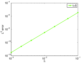
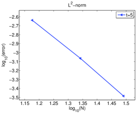
Figure 7.1. Left: $u=x\exp(-\lambda x)\cos(t)$. Right: $f=\cos(x)\exp(-x)\sin(t)$.

(iii). Consider the case $f(x,t)\equiv 0$. Let $\mu=2/3,~{}\lambda=2/3$ in (7.1). The left of the Figure 7.2 exhibits the evolution of the tempered fractional diffusion model with the initial distribution $u_{0}(x)=xe^{-x}$. The right describes the approximate rate by diverse basis ${\mathcal{L}}^{(-\nu,\lambda)}_{n}{(x)}$ at time $t=10$.

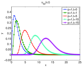
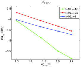
Figure 7.2. TFDEs: $f\equiv 0$, $\lambda=2/3,~{}\mu=2/3.$

8. Tempered fractional diffusion equation on the whole line

In this section, we present a spectral-element method with two-subdomains for the tempered fractional diffusion equation on the whole line originally proposed by [23].

8.1. Tempered fractional diffusion equation

We consider the tempered fractional diffusion equation of order $\mu\in(k-1,k),~{}k=1,2$ on the whole line:

$$\begin{cases}\partial_{t}u(x,t)=(-1)^{k}C_{T}\big{\{}p\partial_{+,x}^{\mu,\lambda}+q\partial_{-,x}^{\mu,\lambda}\big{\}}u(x,t)+f(x,t),\\ u(x,0)=u_{0}(x),\quad\lim_{|x|\rightarrow\infty}u(x,t)=0,\end{cases}$$ (8.1)

where $p,q$ are constants such that $0\leq p,q\leq 1,~{}p+q=1,$ $C_{T}$ is a constant and the fractional operators are

• For $0<\mu<1,$

  $$\partial_{+,x}^{\mu,\lambda}u={{}_{-\infty}}{\rm D}_{x}^{\mu,\lambda}u-\lambda^{\mu}u,\quad\partial_{-,x}^{\mu,\lambda}u={{}_{x}}{\rm D}_{\infty}^{\mu,\lambda}u-\lambda^{\mu}u;$$ (8.2)

• For $1<\mu<2$,

  $$\partial_{+,x}^{\mu,\lambda}u={{}_{-\infty}}{\rm D}_{x}^{\mu,\lambda}u-\mu\lambda^{\mu-1}\partial_{x}u-\lambda^{\mu}u,\quad\partial_{-,x}^{\mu,\lambda}u={{}_{x}}{\rm D}_{\infty}^{\mu,\lambda}u+\mu\lambda^{\mu-1}\partial_{x}u-\lambda^{\mu}u.$$ (8.3)

$$\partial_{\pm,x}^{\mu,\lambda}u=\begin{cases}{}{\rm D}_{\pm}^{\mu,\lambda}u-\lambda^{\mu}u,&0<\mu<1,\\ {}{\rm D}_{\pm}^{\mu,\lambda}u-\pm\mu\lambda^{\mu-1}\partial_{x}u-\lambda^{\mu}u,&1<\mu<2.\end{cases}$$ (8.4)

Here , for notational simplicity, the equivalent notations ${}{\rm D}_{\pm}^{\mu,\lambda}$ are adopted to represent the tempered fractional derivatives as discussed in Remark LABEL:RemNotations.

8.2. A two-domain spectral-element method

Let $\Lambda:=(a,b),-\infty\leq a<b\leq\infty$, and $\omega>0$ be a generic weight function. For any $m\in\mathbb{N}$ and a given weight function $\omega$, we denote

$$H_{\omega}^{m}(\Lambda):=\big{\{}v\in L_{\omega}^{2}(\Lambda):~{}\partial_{x}^{k}v\in L_{\omega}^{2}(\Lambda),~{}0<k\leq m\big{\}}$$

with the semi-norm and norm

$$|v|_{m,\omega,\Lambda}=\|\partial_{x}^{m}v\|_{\omega,\Lambda},\quad\|v\|_{m,\omega,\Lambda}=\Big{(}\sum\limits_{k=0}^{m}|v|^{2}_{k,\omega,\Lambda}\Big{)}^{1/2}.$$

In particular, we omit the subscript $\omega$ when $\omega\equiv 1$.

Moreover, for real $r>0$, we define

$$H^{r,\lambda}(\mathbb{R}):=\big{\{}v\in L^{2}(\mathbb{R}):~{}{{}_{-\infty}}{\rm D}_{x}^{r,\lambda}v\in L^{2}(\mathbb{R})\big{\}}$$

with the semi norm and norm

$$|v|_{r,\lambda}=\|{{}_{-\infty}}{\rm D}_{x}^{r,\lambda}v\|,\quad\|v\|_{r,\lambda}=\big{(}\|v\|^{2}+|v|^{2}_{r,\lambda}\big{)}^{1/2}.$$

A weak formulation of (8.1) is to find $u\in L^{2}\big{(}0,T;H^{1}(\mathbb{R})\cap H^{\mu-k+1,\lambda}(\mathbb{R})\big{)}\cap H^{1}\big{(}0,T;L^{2}(\mathbb{R})\big{)}$ such that

$$\begin{cases}\big{(}\partial_{t}u(\cdot,t),v\big{)}+a^{\mu}_{pq}\big{(}u(\cdot,t),v\big{)}=\big{(}f(\cdot,t),v\big{)},\quad\forall v\in H^{1}(\mathbb{R})\cap H^{\mu-k+1,\lambda}(\mathbb{R}),\\ u(x,0)=u_{0}(x),\end{cases}$$ (8.5)

We decompose the whole line as follows

$$\mathbb{R}={\Lambda}_{1}\cup{\Lambda}_{2},\quad\Lambda_{1}=(-\infty,0),\quad\Lambda_{2}=[0,\infty),$$

and denote $u_{\Lambda_{j}}(x,t):=u(x,t)\big{|}_{\Lambda_{j}},~{}j=1,2$. Introduce the approximation space:

$$V^{\lambda}_{\boldsymbol{N}}({\mathbb{R}}):=\Big{\{}\phi\in C(\mathbb{R})\,:\,\phi_{\Lambda_{i}}(x)=e^{-\lambda|x|}p,\;\;p_{\Lambda_{i}}\in\mathcal{P}_{N_{i}}(\Lambda_{i}),\;\;i=1,2\Big{\}},\quad\boldsymbol{N}=(N_{1},N_{2}),$$ (8.6)

and define

$$\phi^{\ast}(x)=e^{-\lambda|x|},\;\;\phi^{-}_{n_{1}}(x)=\begin{cases}{\mathcal{L}}^{(-1,\lambda)}_{n_{1}}{(-x)},&x\leq 0,\\[4.0pt] 0,&x>0,\end{cases}\;\;\phi^{+}_{n_{2}}(x)=\begin{cases}0,&x\leq 0,\\[4.0pt] {\mathcal{L}}^{(-1,\lambda)}_{n_{2}}{(x)},&x>0,\end{cases}$$ (8.7)

where ${\mathcal{L}}^{(-1,\lambda)}_{n}{(}x)=e^{-\lambda x}xL_{n}^{(1)}(2\lambda x)$. One verifies readily that

$$V^{\lambda}_{\boldsymbol{N}}({\mathbb{R}})={\rm span}\big{\{}\phi^{\ast}(x);\;\;\phi^{-}_{n_{1}}(x),\;\;0\leq n_{1}\leq N_{1}-1;\;\;\phi^{+}_{n_{2}}(x),\;\;0\leq n_{2}\leq N_{2}-1\big{\}}.$$ (8.8)

Then, our semi-discrete spectral-Galerkin method is to find $u_{\boldsymbol{N}}(\cdot,t)\in V^{\lambda}_{\boldsymbol{N}}({\mathbb{R}})$ such that

$$\begin{cases}\big{(}\partial_{t}u_{\boldsymbol{N}}(\cdot,t),v\big{)}+a^{\mu}_{pq}\big{(}u_{\boldsymbol{N}}(\cdot,t),v\big{)}=\big{(}f(\cdot,t),v\big{)},\quad&\forall v\in V^{\lambda}_{\boldsymbol{N}}({\mathbb{R}}),\\[4.0pt] \big{(}u_{\boldsymbol{N}}(\cdot,0),v)=(u_{0},v),\quad&\forall v\in V^{\lambda}_{\boldsymbol{N}}({\mathbb{R}}),\end{cases}$$ (8.9)

where the bilinear form $a^{\mu}_{pq}(\cdot,\cdot)$ is defined by

$$a^{\mu}_{pq}(u,v):=\begin{cases}\quad p({{}_{-\infty}}{\rm D}_{x}^{\mu,\lambda}u,v)+q(u,{{}_{-\infty}}{\rm D}_{x}^{\mu,\lambda}v)-\lambda^{\mu}(u,v),~{}\qquad&0<\mu<1,\\ -\big{\{}p({{}_{-\infty}}{\rm D}_{x}^{\mu-1,\lambda}u,{{}_{x}}{\rm D}_{\infty}^{1,\lambda}v)+q({{}_{x}}{\rm D}_{\infty}^{1,\lambda}u,{{}_{-\infty}}{\rm D}_{x}^{\mu-1,\lambda}v)\big{\}}\\ \qquad\quad\,+\lambda^{\mu}(u,v)+(p-q)\mu\lambda^{\mu-1}(\partial_{x}u,v),~{}~{}\quad&1<\mu<2.\end{cases}$$ (8.10)

We provide below some details of the algorithm.

$$u_{\boldsymbol{N}}(x,t) =c^{\ast}(t)\phi^{\ast}({x})+\sum_{n_{1}=0}^{N_{1}-1}c^{-}_{n_{1}}(t)\phi^{-}_{n_{1}}({x})+\sum_{n_{2}=0}^{N_{2}-1}c^{+}_{n_{2}}(t)\phi^{+}_{n_{2}}({x}),$$ (8.11)

$$u_{\boldsymbol{N}}(x,0) =c^{\ast}_{0}\phi^{\ast}({x})+\sum_{n_{1}=0}^{N_{1}-1}c^{-}_{0,n_{1}}\phi^{-}_{n_{1}}({x})+\sum_{n_{2}=0}^{N_{2}-1}c^{+}_{0,n_{2}}\phi^{+}_{n_{2}}({x}).$$

Let $H(x)$ be the Heaviside function as before. Thanks to the tempered fractional derivative and integral relations with GLFs, and a reflected mapping from positive half line $\mathbb{R}^{+}$ to negative half line $\mathbb{R}^{-}$, we can derive the following identities (see Appendix C):

$$\begin{split}&{{}_{x}}{\rm D}_{\infty}^{1,\lambda}\phi^{\ast}(x)=-2\lambda e^{-\lambda x}H(x),\quad{{}_{x}}{\rm D}_{\infty}^{1,\lambda}\phi^{-}_{n_{1}}(x)=(n_{1}+1){\mathcal{L}}^{(0,\lambda)}_{n_{1}}{(-x)}H(-x),\\[6.0pt] &{{}_{-\infty}}{\rm D}_{x}^{s,\lambda}\phi^{\ast}(x)=\begin{cases}(2\lambda)^{s}e^{\lambda x},&x\leq 0,\\[6.0pt] \dfrac{2\lambda e^{\lambda x}}{\Gamma(1-s)}\displaystyle\int_{x}^{\infty}\dfrac{e^{-2\lambda t}}{t^{s}}{\rm d}t,&x>0,\end{cases}\\[6.0pt] &{{}_{-\infty}}{\rm D}_{x}^{s,\lambda}\phi^{-}_{n_{1}}(x)=\begin{cases}-(2\lambda)^{s-1}(n_{1}+1)L^{(s-1)}_{n_{1}+1}{(-2\lambda x)}e^{\lambda x},&x\leq 0,\\[6.0pt] -e^{\lambda x}\dfrac{{n_{1}}+1}{\Gamma(1-s)}\displaystyle\int_{x}^{\infty}\dfrac{L^{(0)}_{{n_{1}}+1}{(2\lambda(t-x))}e^{-2\lambda t}}{t^{s}}{\rm d}t,&x>0,\end{cases}\\[6.0pt] &{{}_{x}}{\rm D}_{\infty}^{1,\lambda}\phi^{+}_{n_{2}}(x)=-(n_{2}+1){\mathcal{L}}^{(0,\lambda)}_{n_{2}+1}{(x)}H(x),\quad\\[6.0pt] &{{}_{-\infty}}{\rm D}_{x}^{s,\lambda}\phi^{+}_{n_{2}}(x)=\dfrac{\Gamma(n_{2}+2)}{\Gamma(n_{2}+2-s)}x^{1-s}{\mathcal{L}}^{(1-s,\lambda)}_{n_{2}}{(x)}H(x).\end{split}$$ (8.12)

• $${{}_{x}}{\rm D}_{\infty}^{1,\lambda}\phi^{\ast}(x) =\begin{cases}0,&x\leq 0,\\ -2\lambda e^{-\lambda x},&x>0,\end{cases}$$ (8.13)

  $${{}_{x}}{\rm D}_{\infty}^{1,\lambda}\phi^{-}_{n_{1}}(x) =\begin{cases}(n_{1}+1)\breve{\mathcal{L}}^{(0,\lambda)}_{n_{1}}{(-x)},&x\leq 0,\\ 0,&x>0,\end{cases}$$

  $${{}_{x}}{\rm D}_{\infty}^{1,\lambda}\phi^{+}_{n_{2}}(x) =\begin{cases}0,&x\leq 0,\\ -(n_{2}+1)\breve{\mathcal{L}}^{(0,\lambda)}_{n_{2}+1}{(x)},&x>0.\end{cases}$$

• $${{}_{-\infty}}{\rm D}_{x}^{s,\lambda}\phi^{\ast}(x) =\begin{cases}(2\lambda)^{s}e^{\lambda x},&x\leq 0,\\ \dfrac{2\lambda e^{\lambda x}}{\Gamma(1-s)}\int_{x}^{\infty}\dfrac{e^{-2\lambda t}}{t^{s}}{\rm d}t,&x>0,\end{cases}$$ (8.14)

  $${{}_{-\infty}}{\rm D}_{x}^{s,\lambda}\phi^{-}_{n_{1}}(x) =\begin{cases}-(2\lambda)^{s-1}(n_{1}+1)\breve{\mathcal{L}}^{(s-1,\lambda)}_{n_{1}+1}{(-x)},&x\leq 0,\\ -e^{\lambda x}\dfrac{{n_{1}}+1}{\Gamma(1-s)}\int_{x}^{\infty}\dfrac{L^{(0)}_{{n_{1}}+1}{(2\lambda(t-x))}e^{-2\lambda t}}{t^{s}}{\rm d}t,&x>0,\end{cases}$$

  $${{}_{-\infty}}{\rm D}_{x}^{s,\lambda}\phi^{+}_{n_{2}}(x) =\begin{cases}0,&x\leq 0,\\ \dfrac{\Gamma(n_{2}+2)}{\Gamma(n_{2}+2-s)}x^{1-s}\breve{\mathcal{L}}^{(1-s,\lambda)}_{n_{2}}{x},&x>0.\end{cases}$$

9. Numerical Implementation

As the shifted Legendre polynomial and the shifted Laguerre function will be utilized to approximate the solution, we first provide some relevant results which are crucial for the numerical implementation. Here we construct a general theory for orthogonal polynomials. Then (8.9) leads to the system

$$\mathbf{M}\frac{d}{dt}\overrightarrow{{\mathbf{C}}}(t)+\mathbf{A}\overrightarrow{{\mathbf{C}}}(t)=\overrightarrow{{\mathbf{F}}}(t),$$ (9.1)

where

$$\begin{split}&\overrightarrow{{\mathbf{C}}}(t)=\big{(}c^{\ast}(t),\overrightarrow{{\mathbf{C}}}^{-}(t),\overrightarrow{\mathbf{C}}^{+}(t)\big{)}^{T},\qquad\overrightarrow{{\mathbf{F}}}(t)=\big{(}f^{\ast}(t),\overrightarrow{{\mathbf{F}}}^{-}(t),\overrightarrow{\mathbf{F}}^{+}(t)\big{)}^{T},\\ &\overrightarrow{{\mathbf{C}}}^{-}(t)=\big{(}c^{-}_{0}(t),c^{-}_{1}(t),\ldots,c^{-}_{N_{1}-1}(t)\big{)}^{T},\quad\qquad\overrightarrow{{\mathbf{C}}}^{+}(t)=\big{(}c^{+}_{0}(t),c^{+}_{1}(t),\ldots,c^{+}_{N_{2}-1}(t)\big{)}^{T}.\\ &\overrightarrow{{\mathbf{F}}}^{-}(t)=\big{(}f^{-}_{0}(t),f^{-}_{1}(t),\ldots,f^{-}_{N_{1}-1}(t)\big{)}^{T},~{}\,\,\quad\quad\overrightarrow{{\mathbf{F}}}^{+}(t)=\big{(}f^{+}_{0}(t),f^{+}_{1}(t),\ldots,f^{+}_{N_{2}-1}(t)\big{)}^{T}.\\ &f^{\ast}(t)=(f,\phi^{\ast}),\quad f^{-}_{n_{1}}(t)=(f,\phi^{-}_{n_{1}}),\qquad f^{+}_{n_{2}}(t)=(f,\phi^{+}_{n_{2}}),\quad{0\leq n_{i}\leq N_{i}-1},~{}i=1,2,\end{split}$$

and the matrices

$$\mathbf{M}=\left(\begin{array}[]{ccc}\mathbf{M}_{1\times 1}^{(*,*)}&{\mathbf{M}}_{1\times N_{1}}^{(*,-)}&{\mathbf{M}}_{1\times N_{2}}^{(*,+)}\\ \\ {\mathbf{M}}_{N_{1}\times 1}^{(-,*)}&\mathbf{M}_{N_{1}\times N_{1}}^{(-,-)}&\mathbf{M}_{N_{1}\times N_{2}}^{(-,+)}\\ \\ {\mathbf{M}}_{N_{2}\times 1}^{(+,*)}&\mathbf{M}_{N_{2}\times N_{1}}^{(+,-)}&\mathbf{M}_{N_{2}\times N_{2}}^{(+,+)}\\ \end{array}\right),\quad\mathbf{A}=\left(\begin{array}[]{ccc}{\mathbf{A}}_{1\times 1}^{(*,*)}&{\mathbf{A}}_{1\times N_{1}}^{(*,-)}&{\mathbf{A}}_{1\times N_{2}}^{(*,+)}\\ \\ {\mathbf{A}}_{N_{1}\times 1}^{(-,*)}&\mathbf{A}_{N_{1}\times N_{1}}^{(-,-)}&\mathbf{A}_{N_{1}\times N_{2}}^{(-,+)}\\ \\ \mathbf{A}_{{N_{2}}\times 1}^{(+,*)}&\mathbf{A}_{N_{2}\times N_{1}}^{(+,-)}&\mathbf{A}_{N_{2}\times N_{2}}^{(+,+)}\\ \end{array}\right),$$ (9.2)

with the entries

$$\mathbf{M}_{c\times d}^{(a,b)}(i+1,j+1)=(\phi^{b}_{j},\phi^{a}_{i}),\quad\mathbf{A}_{c\times d}^{(a,b)}(i+1,j+1)=a_{pq}^{\mu}(\phi^{b}_{j},\phi^{a}_{i}),$$

$$a,b=*,-,+,\quad c,d=1,N_{1},N_{2},\qquad 0\leq i\leq c-1,\quad 0\leq j\leq d-1,$$

and $\overrightarrow{{\mathbf{C}}}(0)$ is determined by the initial data.

The proof of the tempered derivative relation (8.12), and the detail on the entries of the matrix $\mathbf{A}$ can be found in Appendix C. Base on the semi-discrete scheme (9.1), we further use the third-order explicit Runge-Kutta method in time direction with step size $h=10^{-3}$ to numerically solve the problem.

The derivation of the tempered derivative relation (8.12), and the detail on the entries of the matrixes $\mathbf{M}$ and $\mathbf{A}$ can be found in Appendix C. Base on the semi-discrete scheme (9.1), we further use the third-order explicit Runge-Kutta method in time direction with step size $h=10^{-3}$ to numerically solve the problem. 1. Need some detail on the entries of these matrices. 2. How do you solve the ODE system? By Runge-Kutta? This needs to be specified.

9.1. Numerical results

We solve (8.1) with $C_{T}=1$ and $u_{0}=10e^{-5|x|}$ as the initial distribution by using the method presented in the previous section. We first test the accuracy of our method. In Figure 9.1, we plot the the convergence rate of the spectral method at $T=5$ with fixed time step $h=10^{-3}$, in which $f(x,t)\equiv 0$ and $f(x,t)=\cos{t}~{}e^{-x^{2}}$ are the resource terms of the left and the right respectively. We first test the accuracy of our method. In Figure 9.1, we plot the the convergence rate of the spectral method at $T=5$ with fixed time step $h=10^{-3}$, in which $f(x,t)\equiv 0$ and $f(x,t)=\cos{t}~{}e^{-x^{2}}$ are the resource terms of the left and the right respectively. How do you compute the errors? at a fixed time with small time steps?

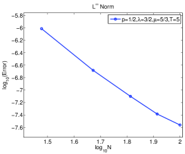
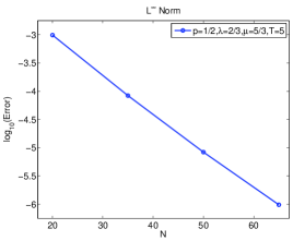
Figure 9.1. Left: $f(x,t)\equiv 0.$  Right: $f(x,t)=\cos{t}~{}e^{-x^{2}}$.

Next, we examine behaviors of the solution under various situations. In Figure 9.2, we plot the snapshots at different times of the tempered fractional diffusion with $p=1/3,~{}q=2/3$ and $p=3/4,~{}q=1/4$, respectively. The case with $p=q=1/2$ is plotted in Figure 9.3.

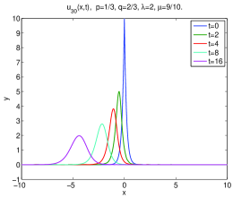
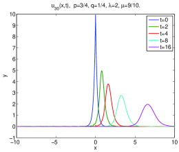
Figure 9.2. Left: $p=1/3,~{}q=2/3.$  Right: $p=3/4,~{}q=1/4.$

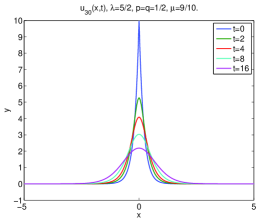
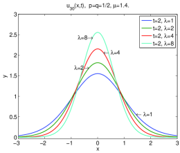
Figure 9.3. Left: $p=q=1/2,~{}\lambda=5/2.$  Right: $p=q=1/2,~{}t=2.$

• The parameters $p$ and $q$ reflect the directional preference of the particle jumping. More precisely, if $p>q$, the particles tend to jump to the right, and if $p<q$, the particles tend to jump to the left, see Figure 9.2. In particular, $p=q$ produces a symmetric profile in the case of $f(x,t)=0$, see the left in Figure 9.3.

  Numerical experiments showed in Figure 9.2 and the left of Figure 9.3 simulate the activities. In particular, when $p=1~{}(q=1)$, the above probability density function of the particles jump indicates that all particles will jump with the right (left) direction which straightforwardly leads to the special case discussed in Subsection 7.1.

• The parameter $\lambda$ determines the probability of the jump distance of the particles. A larger $\lambda$ indicates a shorter jump distance, see the right of Figure 9.3.

• To compare with the usual fractional diffusion equation, i.e., $\lambda=0$, , we plot in Figure 9.4 the particle distributions of the usual fractional diffusion and the tempered fractional diffusion with initial distribution $u_{0}(x)=10e^{-4x^{2}}$ at time $t=10$. We observe that the tail of the tempered fractional diffusion behaves like $|x|^{-\mu-1}e^{-\lambda|x|}$ for large $|x|$ while that that of the usual fractional diffusion behaves like $|x|^{-\mu-1}$.

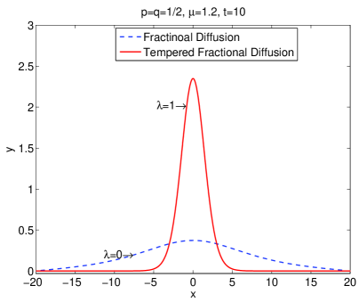
Figure 9.4. Initial distribution $u_{0}(x)=10e^{-4x^{2}}$.

10. Concluding remarks

We presented in this paper efficient spectral methods using the generalized Laguerre functions for solving the tempered fractional differential equations. Our numerical methods and analysis are based on an important observation that the tempered fractional derivative, when restricted to the half line, is intrinsically related to the generalized Laguerre functions that we defined in Sections 3. By exploring the properties of generalized Laguerre functions, we derived optimal approximation results in properly weighted Sobolev spaces, and showed that

we define two classes of generalized Laguerre functions, study their approximation properties, and apply them for solving simple one sided tempered fractional equations. In Section 7, we develop a spectral-Galerkin method for solving a tempered fractional diffusion equation on the half line. Finally, we present a spectral-Galerkin method for solving the tempered fractional diffusion equation on the whole line

Appendix A Properties of Laguerre polynomials

We list below some important properties of Laguerre polynomials (see [26]). For $\alpha>-1$, they are defined by

$$L^{(\alpha)}_{n+1}(x)=\frac{2n+\alpha+1-x}{n+1}L^{(\alpha)}_{n}(x)-\frac{n+\alpha}{n+1}L^{(\alpha)}_{n-1}(x),$$ (A.1)

$$L^{(\alpha)}_{0}(x)=1,\quad L_{1}^{(\alpha)}(x)=-x+\alpha+1.$$

They are eigenfunctions of the Sturm-Liouville problem:

$$x^{-\alpha}e^{x}\partial_{x}\left(x^{\alpha+1}e^{-x}\partial_{x}L_{n}^{(\alpha)}(x)\right)+\lambda_{n}L_{n}^{(\alpha)}(x)=0,\quad\lambda_{n}=n.$$ (A.2)

We have the following relations:

$$L_{n}^{(\alpha)}(x)=\partial_{x}L_{n}^{(\alpha)}(x)-\partial_{x}L_{n+1}^{(\alpha)}(x),$$ (A.3)

$$x\partial_{x}L_{n}^{(\alpha)}(x)=nL_{n}^{(\alpha)}(x)-(n+\alpha)L_{n-1}^{(\alpha)}(x),$$ (A.4)

$$\partial_{x}L_{n}^{(\alpha)}(x)=-L_{n-1}^{(\alpha+1)}(x)=-\sum_{k=0}^{n-1}L_{k}^{(\alpha)}(x).$$ (A.5)

Moreover, we obtain from (A.4) and (A.5) that

$$xL_{n}^{(\alpha+1)}(x)=(n+1+\alpha)L_{n}^{(\alpha)}(x)-(n+1)L_{n+1}^{(\alpha)}(x).$$ (A.6)

Let $\{x_{j}^{(\alpha)}\}_{j=0}^{N}$ be the zeros of $L_{N+1}^{(\alpha)}(x)$. The Laguerre-Gauss quadrature weights are

$$\omega_{j}^{(\alpha)}=\frac{N+\alpha+1}{(N+\alpha+1)N!}\frac{x_{j}^{(\alpha)}}{[L_{N}^{(\alpha)}(x_{j}^{(\alpha)})]^{2}},\quad 0\leq j\leq N.$$ (A.7)

Then we have the exactness of the quadrature rule:

$$\int_{\mathbb{R}^{+}}p(x)x^{\alpha}e^{-x}\,{\rm d}x=\sum_{j=0}^{N}p(x_{j}^{(\alpha)})\omega_{j}^{(\alpha)},\quad\forall\,p\in{\mathbb{P}}_{2N+1}.$$ (A.8)

Appendix B Proof of Lemma 2.2

We first prove (2.55)-(2.56). Recall the fractional integral formula of hypergeometric functions (see [2, P. 287]): for real $b,\mu\geq 0,$

$$x^{b+\mu-1}\,{}_{1}F_{1}(a;b+\mu;x)=\frac{\Gamma(b+\mu)}{\Gamma(b)\Gamma(\mu)}\int_{0}^{x}(x-t)^{\mu-1}t^{b-1}{}_{1}F_{1}(a;b;t)\,{\rm d}t,\quad x\in\mathbb{R}^{+}.$$ (A.1)

Taking $a=-n,~{}b=\alpha+1$ and using the hypergeometric representation (2.47) of the Laguerre polynomials, we obtain

$$x^{\alpha+\mu}L_{n}^{(\alpha+\mu)}(x)=\frac{\Gamma(n+\alpha+\mu+1)}{\Gamma(n+\alpha+1)\Gamma(\mu)}\int_{0}^{x}{(x-t)^{\mu-1}}t^{\alpha}L_{n}^{(\alpha)}(t)\,{\rm d}t,$$

which yields (2.55), i.e.,

$${}_{0}{\rm I}_{x}^{\mu}\{x^{\alpha}L_{n}^{(\alpha)}(x)\}=h_{n}^{\alpha,-\mu}\,x^{\alpha+\mu}\,L_{n}^{(\alpha+\mu)}(x).$$

Then, performing ${{}_{0}}{\rm D}_{x}^{\mu}$ on both sides and taking $\alpha+\mu\to\alpha,$ we derive from the relation (B.9) that for $\alpha-\mu>-1,$

$${{}_{0}}{\rm D}_{x}^{\mu}\{x^{\alpha}L_{n}^{(\alpha)}(x)\}=\frac{1}{h_{n}^{\alpha-\mu,-\mu}}x^{\alpha-\mu}L_{n}^{(\alpha-\mu)}(x)=\frac{\Gamma(n+\alpha+1)}{\Gamma(n+\alpha-\mu+1)}x^{\alpha-\mu}L_{n}^{(\alpha-\mu)}(x).$$

This leads to (2.56).

Lemma 2.1.

Let $\mu\in{\mathbb{R}}^{+}.$

$$\quad{}_{x}{\rm I}_{\infty}^{\mu}\{e^{-x}L_{n}^{(\alpha)}(x)\}=e^{-x}L_{n}^{(\alpha-\mu)}(x),\quad\alpha>\mu-1,$$ (A.2)

$${{}_{x}}{\rm D}_{\infty}^{\mu}\{e^{-x}L_{n}^{(\alpha)}(x)\}=e^{-x}L_{n}^{(\alpha+\mu)}(x),\quad\alpha>-1.$$ (A.3)

Proof.

We now turn to (A.2)-(A.3). According to [20, (6.146), P. 191 ] (or [22, (B-7.2), P. 307]), we have

$${}_{x}{\rm I}_{\infty}^{\mu}\{e^{-x}L_{n}^{(\alpha+\mu)}(x)\}=e^{-x}L_{n}^{(\alpha)}(x),\quad\alpha>-1,~{}\mu>0.$$

Similarly, from the property: ${{}_{x}}{\rm D}_{\infty}^{\mu}{}_{x}{\rm I}_{\infty}^{\mu}\,u(x)=u(x),$ we derive

$${{}_{x}}{\rm D}_{\infty}^{\mu}\{e^{-x}L_{n}^{(\alpha)}(x)\}=e^{-x}L_{n}^{(\alpha+\mu)}(x).$$

Finally, we prove (2.59). Noting that

$$_{1}F_{1}(a;c;x)=e^{x}~{}_{1}F_{1}(c-a;c;-x),$$ (A.4)

(cf. [3, P. 191]), we derive from (2.47) and (A.4) that

$$x^{\alpha} L_{n}^{(\alpha)}(x)e^{-x}=x^{\alpha}\frac{(\alpha+1)_{n}}{n!}~{}{}_{1}F_{1}\big{(}-n;\alpha+1;x\big{)}e^{-x}$$ (A.5)

$$=\frac{(\alpha+1)_{n}}{n!}x^{\alpha}~{}{}_{1}F_{1}\big{(}n+\alpha+1;\alpha+1;-x\big{)}=\frac{(\alpha+1)_{n}}{n!}x^{\alpha}~{}{}_{1}F_{1}\big{(}n+\alpha+1;\alpha+1;-x\big{)}$$

$$=\frac{(\alpha+1)_{n}}{n!}\sum_{j=0}^{\infty}\frac{(n+\alpha+1)_{j}(-1)^{j}}{(\alpha+1)_{j}}\frac{x^{j+\alpha}}{j!}.$$

Then acting the derivative ${}{\rm D}^{k}$ on (A.5) and using the identities (2.47), (A.4) again, we obtain

$${}{\rm D}^{k}\big{\{}x^{\alpha}L_{n}^{(\alpha)}(x)e^{-x}\big{\}} =\frac{(\alpha+1)_{n}}{n!}\sum_{j=0}^{\infty}\frac{(n+\alpha+1)_{j}(-1)^{j}}{(\alpha+1)_{j}}\frac{{}{\rm D}^{k}x^{j+\alpha}}{j!}$$

$$=\frac{(\alpha+1)_{n}}{n!}\sum_{j=0}^{\infty}\frac{(n+\alpha+1)_{j}(-1)^{j}}{(\alpha+1)_{j}}\frac{\Gamma(j+\alpha+1)}{\Gamma(j+\alpha-k+1)}\frac{x^{j+\alpha-k}}{j!}$$

$$=x^{\alpha-k}\frac{(\alpha+1)_{n}}{n!}\frac{\Gamma(\alpha+1)}{\Gamma(\alpha-k+1)}\sum_{j=0}^{\infty}\frac{(n+\alpha+1)_{j}}{(\alpha-k+1)_{j}}\frac{(-x)^{j}}{j!}$$

$$=x^{\alpha-k}\frac{(\alpha-k+1)_{n+k}}{n!}{}_{1}F_{1}\big{(}n+\alpha+1;\alpha-k+1;-x\big{)}$$

$$=\frac{(n+k)!}{n!}x^{\alpha-k}\frac{(\alpha-k+1)_{n+k}}{(n+k)!}{}_{1}F_{1}\big{(}-n-k;\alpha-k+1;x\big{)}e^{-x}$$

$$=\frac{\Gamma(n+k+1)}{\Gamma(n+1)}x^{\alpha-k}L^{(\alpha-k)}_{n+k}(x)e^{-x}.$$

This ends the proof.

Appendix C The proof of (8.12) and the detail on the entries of $\mathbf{A}$

Proof of (8.12)

• for $x\in\mathbb{R}^{-}$, $0<s<1$,

  $${{}_{-\infty}}{\rm D}_{x}^{s,\lambda}\phi^{\ast}(x) ={}_{-\infty}{\rm I}_{x}^{1-s,\lambda}{{}_{-\infty}}{\rm D}_{x}^{1,\lambda}\phi^{\ast}(x)=\frac{e^{-\lambda x}}{\Gamma(1-s)}\int_{-\infty}^{x}\frac{e^{\lambda\tau}(2\lambda)e^{\lambda\tau}}{(x-\tau)^{s}}{\rm d}\tau$$ (B.1)

  $$\overset{t=x-\tau}{=}\frac{2\lambda e^{-\lambda x}}{\Gamma(1-s)}\int_{0}^{\infty}\frac{e^{2\lambda(x-t)}}{t^{s}}{\rm d}t=\frac{(2\lambda)^{s}e^{\lambda x}}{\Gamma(1-s)}\int_{0}^{\infty}e^{-2\lambda t}(2\lambda t)^{-s}{\rm d}(2\lambda t)$$

  $$=(2\lambda)^{s}e^{\lambda x},$$

  $${{}_{-\infty}}{\rm D}_{x}^{s,\lambda}\phi^{-}_{n_{1}}(x) ={}_{-\infty}{\rm I}_{x}^{1-s,\lambda}{{}_{-\infty}}{\rm D}_{x}^{1,\lambda}\phi^{-}_{n_{1}}(x)\overset{\eqref{GLFkderi+-}}{=}{}_{-\infty}{\rm I}_{x}^{1-s,\lambda}\{-({n_{1}}+1){\mathcal{L}}^{(0,\lambda)}_{{n_{1}}+1}{(-x)}\}$$

  $$\overset{\eqref{Laguerreintegralr}}{=}-({n_{1}}+1)(2\lambda)^{s-1}L^{(s-1)}_{{n_{1}}+1}{(-2\lambda x)}e^{-\lambda x}$$

  $${{}_{-\infty}}{\rm D}_{x}^{s,\lambda}\phi^{+}_{n_{2}}(x) =0$$

• for $x\in\mathbb{R}^{+}$, $0<s<1$,

  $${{}_{-\infty}}{\rm D}_{x}^{s,\lambda}\phi^{\ast}(x) ={}_{-\infty}{\rm I}_{x}^{1-s,\lambda}{{}_{-\infty}}{\rm D}_{x}^{1,\lambda}\phi^{\ast}(x)=\frac{e^{-\lambda x}}{\Gamma(1-s)}\int_{-\infty}^{0}\frac{2\lambda e^{2\lambda\tau}}{(x-\tau)^{s}}{\rm d}\tau\overset{\tau=x-t}{=}\frac{2\lambda e^{\lambda x}}{\Gamma(1-s)}\int_{x}^{\infty}\frac{e^{-2\lambda t}}{t^{s}}{\rm d}t,$$ (B.2)

  $${{}_{-\infty}}{\rm D}_{x}^{s,\lambda}\phi^{-}_{n_{1}}(x) ={}_{-\infty}{\rm I}_{x}^{1-s,\lambda}{{}_{-\infty}}{\rm D}_{x}^{1,\lambda}\phi^{-}_{n_{1}}(x)\overset{\eqref{GLFkderi+-}}{=}\frac{e^{-\lambda x}}{\Gamma(1-s)}\int_{-\infty}^{0}\frac{-(n_{1}+1)L^{(0)}_{{n_{1}}+1}{(-2\lambda\tau)}e^{2\lambda\tau}}{(x-\tau)^{s}}{\rm d}\tau$$

  $$\overset{\tau=x-t}{=}-e^{\lambda x}\frac{{n_{1}}+1}{\Gamma(1-s)}\int_{x}^{\infty}\frac{L^{(0)}_{{n_{1}}+1}{(2\lambda(t-x))}e^{-2\lambda t}}{t^{s}}{\rm d}t,$$

  $${{}_{-\infty}}{\rm D}_{x}^{s,\lambda}\phi^{+}_{n_{2}}(x) ={}_{-\infty}{\rm I}_{x}^{1-s,\lambda}{{}_{-\infty}}{\rm D}_{x}^{1,\lambda}\phi^{+}_{n_{2}}(x)\overset{\eqref{GLFkderi++}}{=}\frac{e^{-\lambda x}}{\Gamma(1-s)}\int_{0}^{x}\frac{({n_{2}}+1)L^{(0)}_{{n_{2}}}{(x)}}{(x-\tau)^{s}}{\rm d}\tau$$

  $$=\frac{\Gamma(n_{2}+2)}{\Gamma(n_{2}+2-s)}x^{1-s}{\mathcal{L}}^{(1-s,\lambda)}_{{n_{2}}}{(x)}.$$

• $${{}_{x}}{\rm D}_{\infty}^{1,\lambda}\phi^{\ast}(x) =\begin{cases}0,&x\leq 0,\\ -2\lambda e^{-\lambda x},&x>0,\end{cases}$$ (B.3)

  $${{}_{x}}{\rm D}_{\infty}^{1,\lambda}\phi^{-}_{n_{1}}(x) =\begin{cases}(n_{1}+1)\breve{\mathcal{L}}^{(0,\lambda)}_{n_{1}}{(-x)},&x\leq 0,\\ 0,&x>0,\end{cases}$$

  $${{}_{x}}{\rm D}_{\infty}^{1,\lambda}\phi^{+}_{n_{2}}(x) =\begin{cases}0,&x\leq 0,\\ -(n_{2}+1)\breve{\mathcal{L}}^{(0,\lambda)}_{n_{2}+1}{(x)},&x>0.\end{cases}$$

• $${{}_{-\infty}}{\rm D}_{x}^{s,\lambda}\phi^{\ast}(x) =\begin{cases}(2\lambda)^{s}e^{\lambda x},&x\leq 0,\\ \dfrac{2\lambda e^{\lambda x}}{\Gamma(1-s)}\int_{x}^{\infty}\dfrac{e^{-2\lambda t}}{t^{s}}{\rm d}t,&x>0,\end{cases}$$ (B.4)

  $${{}_{-\infty}}{\rm D}_{x}^{s,\lambda}\phi^{-}_{n_{1}}(x) =\begin{cases}-(2\lambda)^{s-1}(n_{1}+1)\breve{\mathcal{L}}^{(s-1,\lambda)}_{n_{1}+1}{(-x)},&x\leq 0,\\ -e^{\lambda x}\dfrac{{n_{1}}+1}{\Gamma(1-s)}\int_{x}^{\infty}\dfrac{L^{(0)}_{{n_{1}}+1}{(2\lambda(t-x))}e^{-2\lambda t}}{t^{s}}{\rm d}t,&x>0,\end{cases}$$

  $${{}_{-\infty}}{\rm D}_{x}^{s,\lambda}\phi^{+}_{n_{2}}(x) =\begin{cases}0,&x\leq 0,\\ \dfrac{\Gamma(n_{2}+2)}{\Gamma(n_{2}+2-s)}x^{1-s}\breve{\mathcal{L}}^{(1-s,\lambda)}_{n_{2}}{(x)},&x>0.\end{cases}$$

The entries of matrix $\mathbf{A}$ with $1<\mu=1+s<2$. Let $k\in\mathbb{N}$, $k-\nu\leq 0$ and $x\in\mathbb{R}^{-}$. Via the relations (5.5), (5.6) and (2.32), it’s easy to prove that

$${{}_{-\infty}}{\rm D}_{x}^{k,\lambda}\big{\{}{\mathcal{L}}^{(-\nu,\lambda)}_{n}{(-x)}\big{\}}=\frac{\Gamma(n+\nu+1)}{\Gamma(n+\nu-k+1)}~{}{\mathcal{L}}^{(k-\nu,\lambda)}_{n}{(-x)},$$ (B.5)

$$\qquad\quad{{}_{x}}{\rm D}_{\infty}^{k,\lambda}\big{\{}{\mathcal{L}}^{(-\nu,\lambda)}_{n}{(-x)}\big{\}}=(-1)^{k}\frac{\Gamma(n+k+1)}{\Gamma(n+1)}{\mathcal{L}}^{(k-\nu,\lambda)}_{n+k}{(-x)}.\qquad$$ (B.6)

Then,

$$\big{(}{{}_{-\infty}}{\rm D}_{x}^{s,\lambda}\phi^{\ast}, {{}_{x}}{\rm D}_{\infty}^{1,\lambda}\phi^{\ast}\big{)}=\frac{-(2\lambda)^{2}}{\Gamma(1-s)}\int_{0}^{\infty}\int_{x}^{\infty}\frac{e^{-2\lambda t}}{t^{s}}{\rm d}t{\rm d}x=\frac{-(2\lambda)^{2}}{\Gamma(1-s)}\int_{0}^{\infty}\frac{e^{-2\lambda t}}{t^{s}}\int_{0}^{t}1{\rm d}x{\rm d}t$$ (B.7)

$$=\frac{-(2\lambda)^{2}}{\Gamma(1-s)}\int_{0}^{\infty}{t^{1-s}}{e^{-2\lambda t}}{\rm d}t\overset{\tau=2\lambda t}{=}\frac{-(2\lambda)^{s}}{\Gamma(1-s)}\int_{0}^{\infty}{\tau^{1-s}}{e^{-\tau}}{\rm d}\tau=(s-1)(2\lambda)^{s}.$$

Since

$${}{\rm D}\big{\{}(2\lambda x)L^{(1)}_{n_{2}+1}(2\lambda x)\big{\}}=2\lambda(n_{2}+2)L^{(0)}_{n_{2}+1}(2\lambda x),~{}\text{i.e.}~{}\int_{0}^{t}L^{(0)}_{n_{2}+1}(2\lambda x){\rm d}x=\frac{1}{n_{2}+2}tL^{(1)}_{n_{2}+1}(2\lambda t),$$

then,

$$\big{(}{{}_{-\infty}}{\rm D}_{x}^{s,\lambda}\phi^{\ast},{{}_{x}}{\rm D}_{\infty}^{1,\lambda}\phi^{+}_{n_{2}}\big{)} =\frac{-2\lambda(n_{2}+1)}{\Gamma(1-s)}\int_{0}^{\infty}\int_{x}^{\infty}\frac{e^{-2\lambda t}}{t^{s}}{\rm d}t~{}L^{(0)}_{n_{2}+1}(2\lambda x){\rm d}x$$ (B.8)

$${=}\frac{-2\lambda(n_{2}+1)}{\Gamma(1-s)}\int_{0}^{\infty}\frac{e^{-2\lambda t}}{t^{s}}\int_{0}^{t}L^{(0)}_{n_{2}+1}(2\lambda x){\rm d}x~{}{\rm d}t$$

$${=}\frac{-2\lambda(n_{2}+1)}{(n_{2}+2)\Gamma(1-s)}\int_{0}^{\infty}t^{1-s}L^{(1)}_{n_{2}+1}(2\lambda t)e^{-2\lambda t}{\rm d}t.$$

Similarly, we have

$$\big{(}{{}_{-\infty}}{\rm D}_{x}^{s,\lambda}\phi^{-}_{n_{1}},{{}_{x}}{\rm D}_{\infty}^{1,\lambda}\phi^{+}_{n_{2}}\big{)} {=}\frac{({n_{1}}+1)({n_{2}}+1)}{\Gamma(1-s)}\int_{0}^{\infty}\int_{x}^{\infty}\frac{L^{(0)}_{{n_{1}}+1}{(2\lambda(t-x))}e^{-2\lambda t}}{t^{s}}{\rm d}t~{}L^{(0)}_{n_{2}+1}(2\lambda x){\rm d}x$$ (B.9)

$${=} \frac{({n_{1}}+1)({n_{2}}+1)}{\Gamma(1-s)}\int_{0}^{\infty}{t^{-s}}e^{-2\lambda t}\int_{0}^{t}~{}L^{(0)}_{n_{2}+1}(2\lambda x)L^{(0)}_{{n_{1}}+1}{(2\lambda(t-x))}{\rm d}x{\rm d}t$$

$$\overset{x=t\xi}{=} \frac{({n_{1}}+1)({n_{2}}+1)}{\Gamma(1-s)}\int_{0}^{\infty}{t^{1-s}}e^{-2\lambda t}\int_{0}^{1}~{}L^{(0)}_{n_{2}+1}(2\lambda t\xi)L^{(0)}_{{n_{1}}+1}{(2\lambda t(1-\xi))}{\rm d}\xi{\rm d}t.$$

The entries of matrix $\mathbf{A}$ with $0<\mu=s<1$.

$$\big{(}{{}_{-\infty}}{\rm D}_{x}^{s,\lambda}\phi^{\ast},\phi^{\ast}\big{)}=(2\lambda)^{s}\int_{-\infty}^{0}e^{2\lambda x}{\rm d}x+\frac{2\lambda}{\Gamma(1-s)}\int_{0}^{\infty}\int_{x}^{\infty}\frac{e^{-2\lambda t}}{t^{s}}{\rm d}t{\rm d}x$$ (B.10)

$$=(2\lambda)^{s-1}+\frac{2\lambda}{\Gamma(1-s)}\int_{0}^{\infty}\frac{e^{-2\lambda t}}{t^{s}}\int_{0}^{t}1{\rm d}x{\rm d}t=(2\lambda)^{s-1}+\frac{2\lambda}{\Gamma(1-s)}\int_{0}^{\infty}{t^{1-s}}{e^{-2\lambda t}}{\rm d}t$$

$$\overset{\tau=2\lambda t}{=}(2\lambda)^{s-1}+\frac{(2\lambda)^{s-1}}{\Gamma(1-s)}\int_{0}^{\infty}{\tau^{1-s}}{e^{-\tau}}{\rm d}\tau=(2-s)(2\lambda)^{s-1}.$$

Owe to

$${}{\rm D}\big{\{}(2\lambda x)^{2}L^{(2)}_{n_{2}}(2\lambda x)\big{\}}=(2\lambda)^{2}(n_{2}+2)xL^{(1)}_{n_{2}}(2\lambda x),$$

i.e.,

$$\int_{0}^{t}xL^{(1)}_{n_{2}}(2\lambda x){\rm d}x=\frac{1}{n_{2}+2}t^{2}L^{(2)}_{n_{2}}(2\lambda t),$$

we obtain that

$$\big{(}{{}_{-\infty}}{\rm D}_{x}^{s,\lambda}\phi^{\ast},\phi^{+}_{n_{2}}\big{)}=\int_{0}^{\infty}\frac{e^{-\lambda x}}{\Gamma(1-s)}\int_{-\infty}^{0}\frac{2\lambda e^{2\lambda\tau}}{(x-\tau)^{s}}{\rm d}\tau~{}xL^{(1)}_{n_{2}}(2\lambda x)e^{-\lambda x}{\rm d}x$$ (B.11)

$$\overset{\tau=x-t}{=}\frac{2\lambda}{\Gamma(1-s)}\int_{0}^{\infty}\int_{x}^{\infty}\frac{e^{-2\lambda t}}{t^{s}}{\rm d}t~{}xL^{(1)}_{n_{2}}(2\lambda x){\rm d}x{=}\frac{2\lambda}{\Gamma(1-s)}\int_{0}^{\infty}\frac{e^{-2\lambda t}}{t^{s}}\int_{0}^{t}xL^{(1)}_{n_{2}}(2\lambda x){\rm d}x~{}{\rm d}t$$

$$\quad{=}\frac{2\lambda}{(n_{2}+2)\Gamma(1-s)}\int_{0}^{\infty}t^{2-s}L^{(2)}_{n_{2}}(2\lambda t)e^{-2\lambda t}{\rm d}t.$$

Similarly, we have

$$\big{(}{{}_{-\infty}}{\rm D}_{x}^{s,\lambda}\phi^{-}_{n_{1}},\phi^{+}_{n_{2}}\big{)} {=}-\frac{{n_{1}}+1}{\Gamma(1-s)}\int_{0}^{\infty}\int_{x}^{\infty}\frac{L^{(0)}_{{n_{1}}+1}{(2\lambda(t-x))}e^{-2\lambda t}}{t^{s}}{\rm d}t~{}xL^{(1)}_{n_{2}}(2\lambda x){\rm d}x$$ (B.12)

$${=}-\frac{{n_{1}}+1}{\Gamma(1-s)}\int_{0}^{\infty}{t^{-s}}e^{-2\lambda t}\int_{0}^{t}~{}xL^{(1)}_{n_{2}}(2\lambda x)L^{(0)}_{{n_{1}}+1}{(2\lambda(t-x))}{\rm d}x{\rm d}t$$

$$\overset{x=t\xi}{=} -\frac{{n_{1}}+1}{\Gamma(1-s)}\int_{0}^{\infty}{t^{2-s}}e^{-2\lambda t}\int_{0}^{1}~{}\xi L^{(1)}_{n_{2}}(2\lambda t\xi)L^{(0)}_{{n_{1}}+1}{(2\lambda t(1-\xi))}{\rm d}\xi{\rm d}t$$

The above equations are enough to calculate out the matrix $\mathbf{A}$ due to some symmetric properties of the entries.

Appendix D Remain-Liouville and Caputo fractional integrals and derivatives

Recall the definitions of the fractional integrals and fractional derivatives in the sense of Riemann-Liouville (see e.g., [21]).

Definition D.1 (R-L fractional integrals and derivatives).

For $\mu\in{\mathbb{R}}^{+},$ the left and right fractional integrals are respectively defined as

$${}_{a}{\rm I}_{x}^{\mu}f(x)=\frac{1}{\Gamma(\mu)}\int_{a}^{x}\frac{f(y)}{(x-y)^{1-\mu}}dy,\;\;{}_{x}{\rm I}_{b}^{\mu}f(x)=\frac{1}{\Gamma(\mu)}\int_{x}^{b}\frac{f(y)}{(y-x)^{1-\mu}}dy,\;\;\;x\in\Lambda.$$ (B.1)

For real $s\in[k-1,k)$ with $k\in{\mathbb{N}},$ the left-sided Riemann-Liouville fractional derivative (LRLFD) of order $s$ is defined by

$${{}_{a}}{\rm D}_{x}^{s}f(x)=\frac{1}{\Gamma(k-s)}\frac{d^{k}}{dx^{k}}\int_{a}^{x}\frac{f(y)}{(x-y)^{s-k+1}}dy,\;\;\;x\in\Lambda,$$ (B.2)

and the right-sided Riemann-Liouville fractional derivative (RRLFD) of order $s$ is defined by

$${{}_{x}}{\rm D}_{b}^{s}f(x)=\frac{(-1)^{k}}{\Gamma(k-s)}\frac{d^{k}}{dx^{k}}\int_{x}^{b}\frac{f(y)}{(y-x)^{s-k+1}}dy,\;\;\;x\in\Lambda.$$ (B.3)

From the above definitions, it is clear that for any $k\in{\mathbb{N}}_{0},$

$${{}_{x}}{\rm D}_{b}^{k}=(-1)^{k}{}{\rm D}^{k},\quad{{}_{a}}{\rm D}_{x}^{k}={}{\rm D}^{k},\;\;\;{\rm where}\;\;\;{}{\rm D}^{k}:=\frac{d^{k}}{dx^{k}}.$$ (B.4)

Therefore, we can express the RLFD as

$${{}_{a}}{\rm D}_{x}^{s}f(x)={}{\rm D}^{k}\big{\{}{}_{a}{\rm I}_{x}^{k-s}f(x)\big{\}};\quad\;{{}_{x}}{\rm D}_{b}^{s}f(x)=(-1)^{k}{}{\rm D}^{k}\big{\{}{{}_{x}}{\rm D}_{b}^{k-s}f(x)\big{\}}.$$ (B.5)

Due to

$$\frac{1}{\Gamma(\mu)}\int_{\Lambda}\int_{a}^{x}\frac{f(y)}{(x-y)^{1-\mu}}dy\;g(x)dx=\int_{\Lambda}f(y)\frac{1}{\Gamma(\mu)}\int_{x}^{b}\frac{g(x)}{(x-y)^{1-\mu}}dxdy,$$

we can derive the identity

$$({}_{a}{\rm I}_{x}^{\mu}f,g)=(f,{}_{x}{\rm I}_{b}^{\mu}g).$$ (B.6)

Next, we define the Caputo fractional derivatives.

Definition D.2 (Caputo fractional derivatives).

For $s\in[k-1,k)$ with $k\in{\mathbb{N}},$ the left-sided Caputo fractional derivatives (LCFD) of order $s$ is defined by

$${}_{a}^{C}{\rm D}_{x}^{s}f(x):=\frac{1}{\Gamma(k-s)}\int_{a}^{x}\frac{f^{(k)}(y)}{(x-y)^{s-k+1}}dy,\;\;\;x\in\Lambda,$$ (B.7)

and the right-sided Caputo fractional derivatives (RCFD) of order $s$ is defined by

$${}_{x}^{C}{\rm D}_{b}^{s}f(x):=\frac{(-1)^{k}}{\Gamma(k-s)}\int_{x}^{b}\frac{f^{(k)}(y)}{(y-x)^{s-k+1}}dy,\;\;\;x\in\Lambda.$$ (B.8)

According to [10, Thm. 2.14], we have that for any $v\in L^{1}(\Lambda),$ and real $s\geq 0,$

$${{}_{a}}{\rm D}_{x}^{s}\,{}_{a}{\rm I}_{x}^{s}f(x)=f(x),\quad\text{a.e. in}\;\;\Lambda.$$ (B.9)

The following identities shows the relationship between the Riemann-Liouville and Caputo fractional derivatives (see, e.g., [21, Ch. 2]): for $s\in[k-1,k)$ with $k\in{\mathbb{N}},$

$${{}_{a}}{\rm D}_{x}^{s}v(x) ={}_{a}^{C}{\rm D}_{x}^{s}v(x)+\sum_{j=0}^{k-1}\frac{v^{(j)}(a)}{\Gamma(1+j-s)}(x-a)^{j-s};$$ (B.10)

$${{}_{x}}{\rm D}_{b}^{s}v(x) ={}_{x}^{C}{\rm D}_{b}^{s}v(x)+\sum_{j=0}^{k-1}\frac{(-1)^{j}v^{(j)}(b)}{\Gamma(1+j-s)}(b-x)^{j-s}.$$

In the above, the Gamma function with negative, non-integer argument should be understood by the Euler reflection formula (cf. [1]):

$$\Gamma(1+j-s)=\frac{\pi}{\sin(\pi(1+j-s))}\frac{1}{\Gamma(s-j)},\;\;\;s\in(k-1,k),\;\;1\leq j\leq k-2.$$

Note that if $s=k-1,$ then $\Gamma(1+j-s)=\infty$ for all $0\leq j\leq k-2,$ so the summations in the above reduce to $v^{(k-1)}(a)$ and $v^{(k-1)}(b)$ respectively.

For a affine transform $x=\lambda t,~{}\lambda>0$, on account of

$${}_{a}{\rm I}_{t}^{\mu}v(\lambda t) =\frac{1}{\Gamma(\mu)}\int_{a}^{t}\frac{v(\lambda s)}{(t-s)^{1-\mu}}ds=\frac{\lambda^{-\mu}}{\Gamma(\mu)}\int_{a}^{t}\frac{v(\lambda s)}{(\lambda t-\lambda s)^{1-\mu}}\lambda ds$$

$$=\frac{\lambda^{-\mu}}{\Gamma(\mu)}\int_{\lambda a}^{x}\frac{v(y)}{(x-y)^{1-\mu}}dy=\lambda^{-\mu}{}_{\lambda a}{\rm I}_{x}^{\mu}v(x),$$

and

$$\frac{d}{dt}=\frac{dx}{dt}\frac{d}{dx}=\lambda\frac{d}{dx}.$$

Then, due to the definition D.1, it’s easy to derive the below concise identities

$${}_{a}{\rm I}_{t}^{\mu}v(\lambda t)=\lambda^{-\mu}{}_{\lambda a}{\rm I}_{x}^{\mu}v(x),\quad{{}_{a}}{\rm D}_{t}^{s}v(\lambda t)=\lambda^{s}{{}_{\lambda a}}{\rm D}_{x}^{s}v(x),\quad s,\mu,\lambda>0.$$ (B.11)

Similarly, we have the below result for right fractional derivative

$${}_{t}{\rm I}_{b}^{\mu}v(\lambda t)=\lambda^{-\mu}{}_{t}{\rm I}_{\lambda b}^{\mu}v(x),\quad{{}_{t}}{\rm D}_{b}^{s}v(\lambda t)=\lambda^{s}{{}_{x}}{\rm D}_{\lambda b}^{s}v(x),\quad s,\mu,\lambda>0.$$ (B.12)

Appendix E Some Proof

Proof of (B.4) Assume a suitable function $f(x),~{}x\in\mathbb{R}^{+}$, then for any $\mu>0$, its reflection $f(-x),~{}x\in\mathbb{R}^{-}$ satisfies

$${}_{-\infty}{\rm I}_{x}^{\mu,\lambda}f(-x)= \frac{e^{-\lambda x}}{\Gamma(\mu)}\int_{-\infty}^{x}e^{\lambda\tau}(x-\tau)^{\mu-1}f(-\tau){\rm d}\tau\overset{t=-\tau}{=}\frac{e^{-\lambda x}}{{\Gamma(\mu)}}\int^{\infty}_{-x}e^{-\lambda t}(x+t)^{\mu-1}f(t)\rm{\rm d}t$$ (P.1)

$$\overset{y=-x}{=} \frac{e^{\lambda y}}{{\Gamma(\mu)}}\int^{\infty}_{y}e^{-\lambda t}(t-y)^{\mu-1}f(t){\rm d}t={}_{x}{\rm I}_{\infty}^{\mu,\lambda}f(y).$$

Then, recall the result in Lemma 5.1, we have

$$\quad{}_{-\infty}{\rm I}_{x}^{\mu,\lambda}\breve{\mathcal{L}}^{(\alpha,\lambda)}_{n}{(-x)}=(2\lambda)^{-\mu}\breve{\mathcal{L}}^{(\alpha-\mu,\lambda)}_{n}{(-x)},\quad\alpha>\mu-1.$$ (P.2)

In fact,

$${}_{-\infty}{\rm I}_{x}^{\mu,\lambda}\breve{\mathcal{L}}^{(\alpha,\lambda)}_{n}{(-x)}\overset{\eqref{rela+-}}{=}{}_{x}{\rm I}_{\infty}^{\mu,\lambda}\breve{\mathcal{L}}^{(\alpha,\lambda)}_{n}{(y)}\overset{\eqref{TempGLderi1II}}{=}(2\lambda)^{-\mu}\breve{\mathcal{L}}^{(\alpha-\mu,\lambda)}_{n}{(y)}=(2\lambda)^{-\mu}\breve{\mathcal{L}}^{(\alpha-\mu,\lambda)}_{n}{(-x)}.$$

Furthermore, let $k\in\mathbb{N}$, $\alpha>k-1$ and $x\in\mathbb{R}^{-}$. Combining Lemma 5.2 with derivative chain rule leads to

$$\qquad\qquad\quad{{}_{-\infty}}{\rm D}_{x}^{k,\lambda}\big{\{}(-x)^{\alpha}\breve{\mathcal{L}}^{(\alpha,\lambda)}_{n}{(-x)}\big{\}}=(-1)^{k}\frac{\Gamma(n+k+1)}{\Gamma(n+1)}(-x)^{\alpha-k}\breve{\mathcal{L}}^{(\alpha-k,\lambda)}_{n+k}{(-x)}.\qquad$$ (P.3)

Therefore,

• for $x\in\mathbb{R}^{-}$, $0<s<1$,

  $${{}_{-\infty}}{\rm D}_{x}^{s,\lambda}\phi^{\ast}(x) ={}_{-\infty}{\rm I}_{x}^{1-s,\lambda}{{}_{-\infty}}{\rm D}_{x}^{1,\lambda}\phi^{\ast}(x)=\frac{e^{-\lambda x}}{\Gamma(1-s)}\int_{-\infty}^{x}\frac{e^{\lambda\tau}(2\lambda)e^{\lambda\tau}}{(x-\tau)^{s}}{\rm d}\tau$$ (P.4)

  $$\overset{t=x-\tau}{=}\frac{2\lambda e^{-\lambda x}}{\Gamma(1-s)}\int_{0}^{\infty}\frac{e^{2\lambda(x-t)}}{t^{s}}{\rm d}t=\frac{(2\lambda)^{s}e^{\lambda x}}{\Gamma(1-s)}\int_{0}^{\infty}e^{-2\lambda t}(2\lambda t)^{-s}{\rm d}(2\lambda t)$$

  $$=(2\lambda)^{s}e^{\lambda x},$$

  $${{}_{-\infty}}{\rm D}_{x}^{s,\lambda}\phi^{-}_{n_{1}}(x) ={}_{-\infty}{\rm I}_{x}^{1-s,\lambda}{{}_{-\infty}}{\rm D}_{x}^{1,\lambda}\phi^{-}_{n_{1}}(x)\overset{\eqref{GLFkderi-+}}{=}{}_{-\infty}{\rm I}_{x}^{1-s,\lambda}\{-({n_{1}}+1)\breve{\mathcal{L}}^{(0,\lambda)}_{{n_{1}}+1}{(-x)}\}$$

  $$\overset{\eqref{GLFint-+}}{=}-({n_{1}}+1)(2\lambda)^{s-1}\breve{\mathcal{L}}^{(s-1,\lambda)}_{{n_{1}}+1}{(-x)}$$

  $${{}_{-\infty}}{\rm D}_{x}^{s,\lambda}\phi^{+}_{n_{2}}(x) =0$$

• for $x\in\mathbb{R}^{+}$, $0<s<1$,

  $${{}_{-\infty}}{\rm D}_{x}^{s,\lambda}\phi^{\ast}(x) ={}_{-\infty}{\rm I}_{x}^{1-s,\lambda}{{}_{-\infty}}{\rm D}_{x}^{1,\lambda}\phi^{\ast}(x)=\frac{e^{-\lambda x}}{\Gamma(1-s)}\int_{-\infty}^{0}\frac{2\lambda e^{2\lambda\tau}}{(x-\tau)^{s}}{\rm d}\tau$$ (P.5)

  $$\overset{\tau=x-t}{=}\frac{2\lambda e^{\lambda x}}{\Gamma(1-s)}\int_{x}^{\infty}\frac{e^{-2\lambda t}}{t^{s}}{\rm d}t$$

  $${{}_{-\infty}}{\rm D}_{x}^{s,\lambda}\phi^{-}_{n_{1}}(x) ={}_{-\infty}{\rm I}_{x}^{1-s,\lambda}{{}_{-\infty}}{\rm D}_{x}^{1,\lambda}\phi^{-}_{n_{1}}(x)\overset{\eqref{GLFkderi-+}}{=}\frac{e^{-\lambda x}}{\Gamma(1-s)}\int_{-\infty}^{0}\frac{-(n_{1}+1)L^{(0)}_{{n_{1}}+1}{(-2\lambda\tau)}e^{2\lambda\tau}}{(x-\tau)^{s}}{\rm d}\tau$$

  $$\overset{\tau=x-t}{=}-e^{\lambda x}\frac{{n_{1}}+1}{\Gamma(1-s)}\int_{x}^{\infty}\frac{L^{(0)}_{{n_{1}}+1}{(2\lambda(t-x))}e^{-2\lambda t}}{t^{s}}{\rm d}t$$

  $${{}_{-\infty}}{\rm D}_{x}^{s,\lambda}\phi^{+}_{n_{2}}(x) ={}_{-\infty}{\rm I}_{x}^{1-s,\lambda}{{}_{-\infty}}{\rm D}_{x}^{1,\lambda}\phi^{+}_{n_{2}}(x)\overset{\eqref{GLFkderi++}}{=}\frac{e^{-\lambda x}}{\Gamma(1-s)}\int_{0}^{x}\frac{({n_{2}}+1)L^{(0)}_{{n_{2}}}{(x)}}{(x-\tau)^{s}}{\rm d}\tau$$

  $$=\frac{\Gamma(n_{2}+2)}{\Gamma(n_{2}+2-s)}x^{1-s}\breve{\mathcal{L}}^{(1-s,\lambda)}_{{n_{2}}}{(x)}.$$

Calculation for Matrix $\mathbf{A}$ with $1<\mu<2$.

$$\big{(}{{}_{-\infty}}{\rm D}_{x}^{s,\lambda}\phi^{\ast},{{}_{x}}{\rm D}_{\infty}^{1,\lambda}\phi^{\ast}\big{)} =\frac{-(2\lambda)^{2}}{\Gamma(1-s)}\int_{0}^{\infty}\int_{x}^{\infty}\frac{e^{-2\lambda t}}{t^{s}}{\rm d}t{\rm d}x$$ (P.6)

$$=\frac{-(2\lambda)^{2}}{\Gamma(1-s)}\int_{0}^{\infty}\frac{e^{-2\lambda t}}{t^{s}}\int_{0}^{t}1{\rm d}x{\rm d}t$$

$$=\frac{-(2\lambda)^{2}}{\Gamma(1-s)}\int_{0}^{\infty}{t^{1-s}}{e^{-2\lambda t}}{\rm d}t$$

$$\overset{\tau=2\lambda t}{=}\frac{-(2\lambda)^{s}}{\Gamma(1-s)}\int_{0}^{\infty}{\tau^{1-s}}{e^{-\tau}}{\rm d}\tau=(s-1)(2\lambda)^{s}$$

As

$$D\big{\{}(2\lambda x)L^{(1)}_{n_{2}+1}(2\lambda x)\big{\}}=2\lambda(n_{2}+2)L^{(0)}_{n_{2}+1}(2\lambda x),$$

i.e.,

$$\int_{0}^{t}L^{(0)}_{n_{2}+1}(2\lambda x){\rm d}x=\frac{1}{n_{2}+2}tL^{(1)}_{n_{2}+1}(2\lambda t),$$

thus,

$$\big{(}{{}_{-\infty}}{\rm D}_{x}^{s,\lambda}\phi^{\ast},{{}_{x}}{\rm D}_{\infty}^{1,\lambda}\phi^{+}_{n_{2}}\big{)} =\frac{-2\lambda(n_{2}+1)}{\Gamma(1-s)}\int_{0}^{\infty}\int_{x}^{\infty}\frac{e^{-2\lambda t}}{t^{s}}{\rm d}t~{}L^{(0)}_{n_{2}+1}(2\lambda x){\rm d}x$$ (P.7)

$${=}\frac{-2\lambda(n_{2}+1)}{\Gamma(1-s)}\int_{0}^{\infty}\frac{e^{-2\lambda t}}{t^{s}}\int_{0}^{t}L^{(0)}_{n_{2}+1}(2\lambda x){\rm d}x~{}{\rm d}t$$

$${=}\frac{-2\lambda(n_{2}+1)}{(n_{2}+2)\Gamma(1-s)}\int_{0}^{\infty}t^{1-s}L^{(1)}_{n_{2}+1}(2\lambda t)e^{-2\lambda t}{\rm d}t$$

Similarly, we have

$$\big{(}{{}_{-\infty}}{\rm D}_{x}^{s,\lambda}\phi^{-}_{n_{1}},{{}_{x}}{\rm D}_{\infty}^{1,\lambda}\phi^{+}_{n_{2}}\big{)} {=}\frac{({n_{1}}+1)({n_{2}}+1)}{\Gamma(1-s)}\int_{0}^{\infty}\int_{x}^{\infty}\frac{L^{(0)}_{{n_{1}}+1}{(2\lambda(t-x))}e^{-2\lambda t}}{t^{s}}{\rm d}t~{}L^{(0)}_{n_{2}+1}(2\lambda x){\rm d}x$$ (P.8)

$${=} \frac{({n_{1}}+1)({n_{2}}+1)}{\Gamma(1-s)}\int_{0}^{\infty}{t^{-s}}e^{-2\lambda t}\int_{0}^{t}~{}L^{(0)}_{n_{2}+1}(2\lambda x)L^{(0)}_{{n_{1}}+1}{(2\lambda(t-x))}{\rm d}x{\rm d}t$$

$$\overset{x=t\xi}{=} \frac{({n_{1}}+1)({n_{2}}+1)}{\Gamma(1-s)}\int_{0}^{\infty}{t^{1-s}}e^{-2\lambda t}\int_{0}^{1}~{}L^{(0)}_{n_{2}+1}(2\lambda t\xi)L^{(0)}_{{n_{1}}+1}{(2\lambda t(1-\xi))}{\rm d}\xi{\rm d}t$$

Calculation for Matrix $\mathbf{A}$ with $0<\mu<1$.

$$\big{(}{{}_{-\infty}}{\rm D}_{x}^{s,\lambda}\phi^{\ast},\phi^{\ast}\big{)} =(2\lambda)^{s}\int_{-\infty}^{0}e^{2\lambda x}{\rm d}x+\frac{2\lambda}{\Gamma(1-s)}\int_{0}^{\infty}\int_{x}^{\infty}\frac{e^{-2\lambda t}}{t^{s}}{\rm d}t{\rm d}x$$ (P.9)

$$=(2\lambda)^{s-1}+\frac{2\lambda}{\Gamma(1-s)}\int_{0}^{\infty}\frac{e^{-2\lambda t}}{t^{s}}\int_{0}^{t}1{\rm d}x{\rm d}t$$

$$=(2\lambda)^{s-1}+\frac{2\lambda}{\Gamma(1-s)}\int_{0}^{\infty}{t^{1-s}}{e^{-2\lambda t}}{\rm d}t$$

$$\overset{\tau=2\lambda t}{=}(2\lambda)^{s-1}+\frac{(2\lambda)^{s-1}}{\Gamma(1-s)}\int_{0}^{\infty}{\tau^{1-s}}{e^{-\tau}}{\rm d}\tau=(2-s)(2\lambda)^{s-1}$$

Owe to

$$D\big{\{}(2\lambda x)^{2}L^{(2)}_{n_{2}}(2\lambda x)\big{\}}=(2\lambda)^{2}(n_{2}+2)xL^{(1)}_{n_{2}}(2\lambda x),$$

i.e.,

$$\int_{0}^{t}xL^{(1)}_{n_{2}}(2\lambda x){\rm d}x=\frac{1}{n_{2}+2}t^{2}L^{(2)}_{n_{2}}(2\lambda t),$$

we obtain that

$$\big{(}{{}_{-\infty}}{\rm D}_{x}^{s,\lambda}\phi^{\ast},\phi^{+}_{n_{2}}\big{)} =\int_{0}^{\infty}\frac{e^{-\lambda x}}{\Gamma(1-s)}\int_{-\infty}^{0}\frac{2\lambda e^{2\lambda\tau}}{(x-\tau)^{s}}{\rm d}\tau~{}xL^{(1)}_{n_{2}}(2\lambda x)e^{-\lambda x}{\rm d}x$$ (P.10)

$$\overset{\tau=x-t}{=}\frac{2\lambda}{\Gamma(1-s)}\int_{0}^{\infty}\int_{x}^{\infty}\frac{e^{-2\lambda t}}{t^{s}}{\rm d}t~{}xL^{(1)}_{n_{2}}(2\lambda x){\rm d}x$$

$${=}\frac{2\lambda}{\Gamma(1-s)}\int_{0}^{\infty}\frac{e^{-2\lambda t}}{t^{s}}\int_{0}^{t}xL^{(1)}_{n_{2}}(2\lambda x){\rm d}x~{}{\rm d}t$$

$${=}\frac{2\lambda}{(n_{2}+2)\Gamma(1-s)}\int_{0}^{\infty}t^{2-s}L^{(2)}_{n_{2}}(2\lambda t)e^{-2\lambda t}{\rm d}t$$

Similarly, we have

$$\big{(}{{}_{-\infty}}{\rm D}_{x}^{s,\lambda}\phi^{-}_{n_{1}},\phi^{+}_{n_{2}}\big{)} {=}-\frac{{n_{1}}+1}{\Gamma(1-s)}\int_{0}^{\infty}\int_{x}^{\infty}\frac{L^{(0)}_{{n_{1}}+1}{(2\lambda(t-x))}e^{-2\lambda t}}{t^{s}}{\rm d}t~{}xL^{(1)}_{n_{2}}(2\lambda x){\rm d}x$$ (P.11)

$${=}-\frac{{n_{1}}+1}{\Gamma(1-s)}\int_{0}^{\infty}{t^{-s}}e^{-2\lambda t}\int_{0}^{t}~{}xL^{(1)}_{n_{2}}(2\lambda x)L^{(0)}_{{n_{1}}+1}{(2\lambda(t-x))}{\rm d}x{\rm d}t$$

$$\overset{x=t\xi}{=} -\frac{{n_{1}}+1}{\Gamma(1-s)}\int_{0}^{\infty}{t^{2-s}}e^{-2\lambda t}\int_{0}^{1}~{}\xi L^{(1)}_{n_{2}}(2\lambda t\xi)L^{(0)}_{{n_{1}}+1}{(2\lambda t(1-\xi))}{\rm d}\xi{\rm d}t$$

References

- [1] M. Abramovitz and I.A. Stegun. Handbook of Mathematical Functions. Dover, New York, 1972.
- [2] G.E. Andrews, R. Askey, and R. Roy. Special Functions, volume 71 of Encyclopedia of Mathematics and its Applications. Cambridge University Press, Cambridge, 1999.
- [3] George E Andrews, Richard Askey, Ranjan Roy, et al. Special functions, encyclopedia of mathematics and its applications, 1999.
- [4] B. Baeumer, D.A. Benson, M.M. Meerschaert, and S. W Wheatcraft. Subordinated advection-dispersion equation for contaminant transport. Water Resources Research, 37(6):1543–1550, 2001.
- [5] B. Baeumer, M. Kovács, and M.M. Meerschaert. Fractional reproduction-dispersal equations and heavy tail dispersal kernels. Bulletin of Mathematical Biology, 69(7):2281–2297, 2007.
- [6] Peter Carr, Hélyette Geman, Dilip B Madan, and Marc Yor. The fine structure of asset returns: An empirical investigation*. The Journal of Business, 75(2):305–333, 2002.
- [7] Sheng Chen, Jie Shen, and Li-Lian Wang. Generalized Jacobi functions and their applications to fractional differential equations. Math. Comp., 85(300):1603–1638, 2016.
- [8] J.H. Cushman and T.R. Ginn. Fractional advection-dispersion equation: a classical mass balance with convolution-fickian flux. Water resources research, 36(12):3763–3766, 2000.
- [9] Z.Q. Deng, L. Bengtsson, and V.P. Singh. Parameter estimation for fractional dispersion model for rivers. Environmental Fluid Mechanics, 6(5):451–475, 2006.
- [10] Kai Diethelm. The Analysis of Fractional Differential Equations, Lecture Notes in Math., Vol. 2004. Springer, Berlin, 2010.
- [11] R. Gorenflo, F. Mainardi, E. Scalas, and M. Raberto. Fractional calculus and continuous-time finance iii: the diffusion limit. In Mathematical finance, pages 171–180. Springer, 2001.
- [12] Can Huang, Qingshuo Song, and Zhimin Zhang. Spectral collocation method for substantial frac- tional di erential equations. Submitted.
- [13] J.H. Jeon, H.M.S. Monne, M. Javanainen, and R. Metzler. Anomalous diffusion of phospholipids and cholesterols in a lipid bilayer and its origins. Physical review letters, 109(18):188103, 2012.
- [14] M. Magdziarz, A. Weron, and K. Weron. Fractional fokker-planck dynamics: Stochastic representation and computer simulation. Physical Review E, 75(1):016708, 2007.
- [15] Mark M Meerschaert, Yong Zhang, and Boris Baeumer. Tempered anomalous diffusion in heterogeneous systems. Geophysical Research Letters, 35(17), 2008.
- [16] M.M. Meerschaert and E. Scalas. Coupled continuous time random walks in finance. Physica A: Statistical Mechanics and its Applications, 370(1):114–118, 2006.
- [17] R. Metzler and J. Klafter. The random walk’s guide to anomalous diffusion: a fractional dynamics approach. Physics Reports, 339(1):1–77, 2000.
- [18] R. Metzler and J. Klafter. The restaurant at the end of the random walk: recent developments in the description of anomalous transport by fractional dynamics. Journal of Physics A: Mathematical and General, 37(31):R161, 2004.
- [19] A Piryatinska, A. Saichev, and W. Woyczynski. Models of anomalous diffusion: the subdiffusive case. Physica A: Statistical Mechanics and its Applications, 349(3):375–420, 2005.
- [20] I. Podlubny. Fractional Differential Equations, volume 198 of Mathematics in Science and Engineering. Academic Press Inc., San Diego, CA, 1999. An introduction to fractional derivatives, fractional differential equations, to methods of their solution and some of their applications.
- [21] I. Podlubny. Fractional differential equations: an introduction to fractional derivatives, fractional differential equations, to methods of their solution and some of their applications. Academic press, 1999.
- [22] G. Y. Popov. Concentration of elastic stresses near punches, cuts, thin inclusions and supports. Nauka, Moscow, 1:982, 1982.
- [23] F. Sabzikar, M.M. Meerschaert, and J. Chen. Tempered fractional calculus. Journal of Computational Physics, 2014.
- [24] S.G. Samko, A.A. Kilbas, and O.I. Maričev. Fractional integrals and derivatives. Gordon and Breach Science Publ., 1993.
- [25] E. Scalas. Five years of continuous-time random walks in econophysics. In The complex networks of economic interactions, pages 3–16. Springer, 2006.
- [26] J. Shen, T. Tang, and L.L. Wang. Spectral Methods: Algorithms, Analysis and Applications, volume 41 of Series in Computational Mathematics. Springer-Verlag, Berlin, Heidelberg, 2011.
- [27] E.M. Stein and G.L. Weiss. Introduction to Fourier analysis on Euclidean spaces, volume 1. Princeton university press, 1971.
- [28] G. Szegö. Orthogonal Polynomials (Fourth Edition). AMS Coll. Publ., 1975.
- [29] Mohsen Zayernouri, Mark Ainsworth, and George Em Karniadakis. Tempered fractional Sturm-Liouville eigenproblems. SIAM J. Sci. Comput., 37(4):A1777–A1800, 2015.
- [30] C. Zhang and B.Y. Guo. Domain decomposition spectral method for mixed inhomogeneous boundary value problems of high order differential equations on unbounded domains. Journal of Scientific Computing, 53(2):451–480, 2012.
- [31] Yong Zhang and Mark M Meerschaert. Gaussian setting time for solute transport in fluvial systems. Water Resources Research, 47(8), 2011.