PAL-Hom method for QP and an application to LP

Abstract

In this paper, a proximal augmented Lagrangian homotopy (PAL-Hom) method for solving convex quadratic programming problems is proposed. This method takes the proximal augmented Lagrangian method as the outer iteration. To solve the proximal augmented Lagrangian subproblems, a homotopy method is presented as the inner iteration. The homotopy method tracks the piecewise-linear solution path of a parametric quadratic programming problem whose start problem takes an approximate solution as its solution and the target problem is the subproblem to be solved. To improve the performance of the homotopy method, the accelerated proximal gradient method is used to obtain a fairly good approximate solution that implies a good prediction of the optimal active set. Moreover, a sorting technique for the Cholesky factor update as well as an $\varepsilon$-relaxation technique for checking primal-dual feasibility and correcting the active sets are presented to improve the efficiency and robustness of the homotopy method. Simultaneously, a proximal-point-based AL-Hom method which is shown to converge in finite number of steps, is applied to linear programming. Numerical experiments on randomly generated problems and the problems from the CUTEr and Netlib test collections, support vector machines (SVMs) and contact problems of elasticity demonstrate that PAL-Hom is faster than the active-set methods and the parametric active set methods and is competitive to the interior-point methods and the specialized algorithms designed for specific models (e.g., sequential minimal optimization (SMO) method for SVMs).

1 Introduction

In this paper, we consider the convex quadratic programming (QP) problem

$$\begin{array}[]{l}\min~{}~{}\frac{1}{2}x^{T}Qx+r^{T}x\\ \rm{s.t.}~{}~{}~{}\emph{Ax}=\emph{b},\\ ~{}~{}~{}~{}~{}~{}~{}\emph{x}\geq 0,\end{array}$$ (1)

where $Q$ is an $n\times n$ symmetric semipositive definite matrix, $A$ is an $m\times n$ matrix, $r$ is an $n$-dimensional vector and $b$ is an $m$-dimensional vector.

As a type of classical optimization problem, QP problems arise in many areas, e.g., finance cornuejols2006optimization and optimal control dostal2000solution ; dostal2000duality . In particular, the QP problem is a key issue in support vector machines (SVMs) CC01a . Due to their broad applicability, QP problems have attracted an enormous amount of research on developing efficient algorithms. Among the typical methods for QP problems, interior-point methods (IPMs) karmarkar1984new ; wright1997primal ; mehrotra1992implementation ; zhang1998solving and active-set (AS) methods fletcher1971general ; fletcher2000stable ; gould1991algorithm ; forsgren2016primal ; gill2015methods are two important types of methods and have been implemented in many software packages, e.g., CPLEX, Gurobi, MATLAB, IPOPTwachter2006implementation , QPOPT gill1995user , and SNOPTgill2008user . AS methods are efficient for solving small- to medium-scale QPs, and generally, they can obtain high-precision solutions. Compared with AS methods, IPMs are shown to be more efficient for large-scale QP problems.

In addition to these two classical methods, the augmented Lagrangian method (ALM) is another well-known method and was proposed independently by Hestenes hestenes1969multiplier and Powell powell1969method for nonlinear programming with general constraints and simple bounds. Simultaneously, Powell provided a global convergence analysis that requires the exact minimization of the subproblems. However, Rockafellar rockafellar1976augmented , Bertsekas bertsekas1999nonlinear and Conn et al. conn1991globally showed that the exact minimization is not necessary for convergence. Moreover, a superlinear convergence analysis of the ALM that exactly solves the subproblems and has a new Lagrangian multipliers updating formula was presented by Yuan yuan2014analysis . Besides the theory results, Conn presented an effective numerical implementation of the ALM that exactly asymptotically solved the subproblems in LANCELOT software conn2013lancelot .

Dostal et al. used the ALM dostal2003augmented to solve QP problems $(\ref{scqp})$, which follows Conn et al. conn1991globally who used the ALM to solve general nonlinear constrained optimization problems. The $k$-th iteration of the ALM for $(\ref{scqp})$ begins with a given $\lambda^{k}$ and obtains $(x^{k+1},~{}\lambda^{k+1})$ via

$$x^{k+1} = \arg\min~{}\{\mathcal{L}_{\beta}(x,\lambda^{k})~{}|~{}x\geq 0\},$$ (2)

$$\lambda^{k+1} = \lambda^{k}-\beta(Ax^{k+1}-b).$$

where

$$\mathcal{L}_{\beta}(x,\lambda)=\frac{1}{2}x^{T}Qx+r^{T}x-\lambda^{T}(Ax-b)+\frac{\beta}{2}\Arrowvert Ax-b\Arrowvert^{2}$$

is the augmented Lagrangian function of $(\ref{scqp})$ (omitting the $x\geq 0$ bounds). The performance of the ALM depends on the solving of the subproblems (2). Therefore, it is desired to design efficient algorithms for the augmented Lagrangian subproblems.

The parametric active-set (PAS) method is a type of AS method proposed by Ritter ritter1967method ; ritter1981parametric and Best best1982algorithm ; best1996algorithm for the parametric quadratic programming (PQP) problem

$$\begin{array}[]{l}\min~{}\{(r+tq)^{T}x+\frac{1}{2}x^{T}Q{x}|~{}g+tp\leq Bx\}\end{array}$$ (3)

where $p$ and $q$ are $n$-vectors, $g$ is an $m$-vector, and $B$ is an $m\times n$ matrix. Ferreau et al. ferreau2008online applied the PAS method to the model predictive control problem by solving a sequence of PQP problems with the PAS method. The PQP problems are constructed such that the starting solution of the current PQP problem occurs as the target solution of the previous PQP problem. Furthermore, Ferreau et al. used the PAS method to solve the general convex QP problem

$$\begin{array}[]{l}\min~{}\{r^{T}x+\frac{1}{2}x^{T}Q{x}|~{}g\leq Bx,\}\end{array}$$ (4)

(It is clear that the QP problem (1) can be transformed into the form (4)) by tracking the piecewise-linear solution path of the following PQP problem

$$\begin{array}[]{l}\min~{}\{r(t)^{T}x+\frac{1}{2}x^{T}Q{x}|~{}g(t)\leq Bx\}\end{array}$$ (5)

from $t=1$ to $t=0$, which has been implemented in the software package qpOASES ferreau2014qpoases . The PQP problem in (5) is constructed such that (I) when $t=0$, it becomes (4), that is, $r(0)=r,g(0)=g$; (II) when $t=1$, its solution $x(1)$ as well as the corresponding multipliers $\lambda(1)\geq 0$ with $g(1)\leq Bx(1)$, $\lambda(1)^{T}(g(1)-Bx(1))=0$ and $r(1)=-Qx(1)+B^{T}\lambda(1)$ are known.

At every step of PAS, it needs to solve the linear systems

$$\left[\begin{array}[]{cc}Q&B_{\mathcal{A}}^{T}\\ B_{\mathcal{A}}&0\end{array}\right]\left[\begin{array}[]{c}x(t)\\ \lambda_{\mathcal{A}}(t)\end{array}\right]=\left[\begin{array}[]{c}-r(t)\\ g_{\mathcal{A}}(t)\end{array}\right],$$ (6)

which are derived from the Karush-Kuhn-Tucker (KKT) conditions, where $\mathcal{A}$ denotes the active set. AS methods change the active set along the descent directions, while PAS changes along the parameter $t$ from $t=1$ to $t=0$. The number of steps of the PAS is generally smaller than that in the AS method. In fact, the number of steps in the PAS is close to the number of the different members between the starting active set and the target active set. Therefore, the efficiency of the PAS method depends on the number of active constraints which determines the size of (6), and the difference between the starting active set and the target active set. When the starting active set and the target active set are close, PAS needs a small number of steps to obtain the exact solution. Therefore, a good warm-wart technique for the PAS method is very important to the high performance of PAS. Compared with AS methods, the number of steps in the PAS method is not affected by the distribution of the eigenvalues of $Q$. Specifically, if $Q$ has only a small number of large eigenvalues and if the other eigenvalues are close to zero, AS methods may be inefficient.

Because the main computation of the ALM is to solve the subproblems (2) (which are special cases of (4) with $B=I$), and because PAS is efficient at obtaining an exact solution of (2) (when a good prediction of the optimal active is given), we combine ALM and PAS to solve the QP problem (1). Benefiting from the framework of the ALM, the size of the KKT systems in the combined method is close to the number of free variables at the solution. Therefore, the scale of the KKT systems in the combinational algorithm is smaller than that in the PM, AS and original PAS methods; this is especially significant when the solutions are sparse.

Furthermore, as mentioned in conn1991globally ; dostal2003augmented , it does not always need to obtain high-precision solutions of the subproblems; thus, we use a first-order algorithm to approximately solve the augmented Lagrangian subproblems at the early stage of the augmented method. As $k$ increases, the precision of the solutions of the subproblems is required to be higher. The first-order algorithms are generally efficient at obtaining approximate solutions. However, they needs substantially much more computation to achieve high-precision solutions. Therefore, we plan to use the PAS algorithm to obtain the exact solutions of the augmented Lagrangian subproblems at the mid to late stages.

However, the PAS method needs to retain the invertibility of the KKT systems in the tracking steps. If the PAS method is applied to solve (1) directly and if $Q$ is positive definite, an addition or removal of a constraint may lead to a loss of invertibility. In qpOASES, Ferreau et al. retain the invertibility in Eq. (6) by exchanging an index of the active set and inactive set. Fortunately, based on the framework of the ALM, the augmented Lagrangian subproblems have only bound constraints; therefore, if $Q$ is positive definite, then the Hessian matrices of $\mathcal{L}_{\beta}(x,\lambda^{k})$ are positive definite, which implies that the KKT systems in the homotopy tracking steps would always be invertible. Thus, we do not need to exchange indices to ensure the invertibility of the KKT systems, as is the case in qpOASES. Moreover, when $Q$ is not positive definite, we add proximal terms to the objective function of the augmented Lagrangian subproblems as follows

$$\begin{array}[]{l}x^{k+1}=\arg\min~{}\{\mathcal{L}_{\beta}(x,\lambda^{k})+\frac{d_{k}}{2}\|x-x^{k}\|^{2}~{}|~{}x\geq 0\}.\end{array}$$ (7)

Thus the Hessian matrices of the subproblems are positive definite.

Because the PAS method is essentially a homotopy-like method for PQP, we use homotopy to denote the simplified PAS method and use AL-Hom to denote the ALM with every subproblem solved by the homotopy algorithm. Accordingly, we use PAL-Hom to denote the proximal ALM with the homotopy algorithm solving the subproblems.

Unfortunately, a simple combination of the ALM and the homotopy algorithm is unsatisfactory for QP problems (1). An efficient implementation of the homotopy algorithm needs a good warm start for the homotopy algorithm as well as a fast Cholesky factor update. Moreover, although the invertibility can be ensured by the above processes, a large condition number of (6) leads to large changes in the solution, which would lead to incorrect updates of the active set. In addition, the lack of strict complementarity would also lead to incorrect updates. For these reasons, we present three important techniques: an accelerated proximal gradient method for warm starts; a sorting technique for the Cholesky factorization update, and an $\varepsilon$-precision verification and correction technique to correct incorrect updates of the active set.

Because the efficiency of the homotopy algorithm depends on the difference between the starting active set and the target active set, it is important to design a good warm-start technique to obtain a good estimate of the optimal active set. In the implementation of PAS, the authors have not provided methods to predict the optimal active set and just used the solution of a previous subproblem which may be not a good warm start. When PAS is directly applied to solve problems (1), the performance is unsatisfactory because for general QP problems, it is not easy to predict the active set of (1). Fortunately, based on the framework of the ALM, it is much easier to design a warm start for PAL-Hom which iteratively solves the proximal augmented Lagrangian subproblems.

It is well known that Nesterov’s accelerated proximal gradient (APG) nesterov2005smooth ; nesterov2007gradient algorithm is able to handle very-large-scale problems and converges at a rate $O(\frac{1}{k^{2}})$ which is fast for first-order algorithms. In particular, for the augmented Lagrangian subproblems, the APG is easily implemented and has a low computational complexity at every iteration. Moreover, the APG allows for a rapid change in the active set at every iteration. For these reasons, we use APG to predict the optimal active set of the augmented Lagrangian subproblem. Fortunately, a low-precision solution of (7) often implies a good estimate of the optimal active set; when an approximate solution that provides a good estimate of the optimal active set is given, the homotopy algorithm needs a small number of steps to obtain an exact solution.

Simultaneously, to improve the efficiency and robustness of the homotopy algorithm, we present a sorting technique for the Cholesky factorization update (Section 2.3) that requires fewer computations than the Cholesky factorization update in qpOASES, as well as an $\varepsilon$-precision verification and a correction technique (Section 2.4) to address the incorrect updates of the active set caused by the lack of strict complementarity and the computation errors in solving the linear systems.

The outline of the remainder of this paper is as follows. Details of the homotopy algorithm are presented in Section 2. In Section 3, we apply a proximal- point-based AL-Hom to solve linear programming (LP) problems and prove that it converges in a finite number of iterations. Moreover, an estimate of the maximum number of iterations and a lower bound on the descent of the linear objective are given. Finally, the numerical results for QPs and LPs from synthetic data and real-world data are presented in Section 4.

2 Homotopy algorithm for the subproblems of ALM

In this section, we follow Conn et al. dostal2003augmented and Dostal et al. conn1991globally using the ALM to solve the QP problem (1); however, we add proximal terms into the objective of the augmented Lagrangian subproblems to obtain the strict convexity of the subproblems. Moreover, because the main computation of the proximal augmented Lagrangian method is solving the augmented Lagrangian subproblems, we present a homotopy algorithm for exactly solving the subproblems with a uniform form

$$\begin{array}[]{l}\min~{}\{f^{T}z+\frac{1}{2}z^{T}H{z}|z\geq 0\},\end{array}$$ (8)

where $H=Q+d_{k}I+\beta A^{T}A$ (if $Q$ is positive definite, $d_{k}=0$) is positive definite and $f=r-A^{T}\lambda^{k}-\beta A^{T}b-d_{k}x^{k}$. As mentioned in the introduction, the homotopy algorithm is a simplified PAS method, and is improved with three important techniques: warm start, Cholesky factorization update and $\varepsilon$-precision verification and correction.

Before presenting the homotopy algorithm, we give the optimality conditions of (8) as follows, where $z^{*}$ is the solution of (8) if and only if

$$Hz^{*}+f\geq 0,$$ (9)

$$z^{*}\geq 0,$$ (10)

$${z^{*}}^{T}(Hz^{*}+f)=0,$$ (11)

2.1 Warm start

Because the homotopy algorithm needs a good estimate of the optimal active set of (8), and because the APG algorithm efficiently obtains an approximate solution of (8), which often implies a good estimate of the optimal active set, we implement APG to approximately solve (8).

Let $z^{1}=y^{0}$ which is pregiven, $l=1$, and $\theta_{1}=1$; then, APG iterates as follows.

$$y^{l}=\arg\min_{z\geq 0}\langle Hz^{l}+f,z\rangle+\frac{L}{2}\Arrowvert z-z^{l}\Arrowvert^{2},$$ (12)

$$\theta_{l+1}=\frac{1+\sqrt{1+4\theta_{l}^{2}}}{2},$$ (13)

$$z^{l+1}=y^{l}+(\frac{\theta_{l}-1}{\theta_{l+1}})(y^{l}-y^{l-1}),$$ (14)

where $L\geq\Arrowvert H\Arrowvert$. In each iteration, $(\ref{apg step1})$ can be solved by a truncation operator

$$\begin{array}[]{l}y^{l}=T(z^{l}-\frac{1}{L}(Hz^{l}+f))=[z^{l}-\frac{1}{L}(Hz^{l}+f)]_{+}.\end{array}$$

Hence, the main computation at each iteration is a matrix-vector multiplication.

Because a low-precision solution often implies a good estimate of the optimal active set and because APG is slow at the end of the iterations, we terminate the APG algorithm when $y^{l}$ satisfies one of the following criteria.

$$\mu_{\varepsilon_{1}}(y^{l})=\mu_{\varepsilon_{1}}(y^{l-i}),~{}for~{}i=1,..,S_{\max},$$ (15)

$$\frac{\Arrowvert y^{l}-y^{l-1}\Arrowvert}{\Arrowvert y^{l}\Arrowvert}<\varepsilon_{2},$$ (16)

where $\mu_{\varepsilon_{1}}(y)=\Arrowvert[y-\|y\|\varepsilon_{1}]_{+}\Arrowvert_{0}$, $S_{\max}$, $\varepsilon_{1}$ and $\varepsilon_{2}$ are some parameters that are given. Because the index $i$ is likely to be active if $y^{l}_{i}<\eta\Arrowvert y^{l}\Arrowvert$, we truncate $y^{l}$ with $\eta\Arrowvert y^{l}\Arrowvert$ as follows

$$\begin{array}[]{l}\hat{z}=\left\{\begin{array}[]{lcl}y_{j}^{l},\hskip 28.45274pty_{j}^{l}\geq\eta\Arrowvert y^{l}\Arrowvert\\ 0,\hskip 34.14322ptelse\\ \end{array}\right.\end{array}$$ (17)

where $\eta>0$. Let

$$w=\left\{\begin{array}[]{lcl}-H_{j}^{T}\hat{z}-f_{j},&&{\hat{z}_{j}>0},\\ \xi,&&{\hat{z}_{j}=0},\end{array}\right.$$ (20)

where $\xi=-\min_{j}\{H_{j}^{T}\hat{z}+f_{j}|\hat{z}_{j}=0\}+\delta_{1}$ and $\delta_{1}>0$. Therefore, we have that $\hat{z}$ is the solution of

$$\begin{array}[]{l}\min~{}~{}\frac{1}{2}z^{T}Hz+(f+w)^{T}z\\ \rm{s.~{}t.}~{}~{}~{}\emph{z}\geq 0.\end{array}$$ (21)

from (9)-(11).

2.2 Homotopy tracking

The linear homotopy between the objective function of $(\ref{almsub})$ and $(\ref{warm start})$ is

$$\begin{array}[]{l}h(t,z)=\frac{1}{2}z^{T}Hz+(f+tw)^{T}z~{},~{}t\in[0,1].\end{array}$$

Then we can obtain the solution of $(\ref{almsub})$ by tracking the piecewise-linear solution path of the PQP problem

$$\begin{array}[]{l}\min~{}~{}h(t,z)=\frac{1}{2}z^{T}Hz+(f+tw)^{T}z\\ \rm{s.~{}t.}~{}~{}~{}\emph{z}\geq 0.\end{array}$$ (22)

Let $z(t)$, $t\in[0,1]$ be a vector function of $t$ denoting the solution path of (22). Suppose $z(t)$ is linear in $M$ intervals, and set $t_{0}=1,t_{M}=0$. Let $(t_{i},t_{i-1})$, $i=1,...,M$ denote the intervals, in which $z(t)$ is linear. Moreover, let $J(z(t))=\{j|H^{T}_{j}z(t)+f_{j}+tw_{j}=0\}$ denote the working set. Because $z(t)$ is piecewise-linear, $J(z(t))$ is constant in every interval. We use $J^{i}=\{J(z(t))|t\in(t_{i},t_{i-1})\}$ to denote the working set in the $i$-th interval, and we let $J^{i}_{c}=\{1,...,n\}\backslash J^{i}$.

Proposition 1

For any $i\in\{1,...,M\}$, there exists only one index set $S^{i}\subset\{1,...,n\}$ such that

$$z_{S^{i}}(t)=-H_{S^{i}S^{i}}^{-1}(f_{S^{i}}+tw_{S^{i}})\geq 0,$$ (23)

$$z_{S^{i}_{c}}(t)=0,$$ (24)

$$H^{T}_{S^{i}_{c}}z(t)+f_{S^{i}_{c}}+tw_{S^{i}_{c}}>0$$ (25)

holds for any $t\in(t_{i},t_{i-1})$, where $S^{i}_{c}=\{1,...,n\}\backslash S^{i}$, $H_{S^{i}S^{i}}$ and $H_{S^{i}_{c}S^{i}}$ denote the submatrices of $H$ with appropriate rows and columns.

$Proof.$ Clearly, if $S^{i}$ satisfies $(\ref{kkt1})$-$(\ref{kkt3})$, then $z(t)$ is the solution of (22) at $t$. Moreover, because $H$ is positive definite, for any $t$, the solution of (22) is unique. Then, we have that $J^{i}$ is the unique index set, which satisfies $(\ref{kkt1})$-$(\ref{kkt3})$.

The essence of the homotopy tracking steps is to calculate the solution path $z(t)$ that is unique from $t=1$ to $t=0$. This is equivalent to updating $J^{i}$ and $J_{c}^{i}$ from $t=1$ to $t=0$. Therefore, if a good prediction of the optimal active set is obtained, that is, $J(1)$ is close to $J(0)$, a small number of update steps is needed to change $J(1)$ to $J(0)$. Benefiting from the approximate solution from APG, $\hat{z}$ is an approximate solution of $(\ref{almsub})$, and the starting active set is hopefully close to the target active set; this implies that the number of steps of the subsequent iterations is hopefully small.

We start the homotopy tracking steps with $z(t_{0})=\hat{z}$, $J^{1}=\{j|\hat{z}_{j}>0\}$ and $J^{1}_{c}=\{1,...,n\}\backslash J^{1}$. In the homotopy tracking steps, we need to calculate $t_{i}$ and update the working set $J^{i+1}$ for $i=1,2,..M-1$.

From Proposition 1, $z(t)$ has the closed form

$$z_{J^{i}}(t) = -H_{J^{i}J^{i}}^{-1}(f_{J^{i}}+tw_{J^{i}}),$$ (26)

$$z_{J^{i}_{c}}(t) = 0$$ (27)

in the $i$-th interval. We continue to decrease $t$ starting at $t_{i-1}$ until one of the following events occurs.

1. There exists $j\in J^{i}$ and $\tilde{t}<t_{i-1}$ such that $z_{j}(t)>0,t\in(\tilde{t},t_{i-1})$ and $z_{j}(\tilde{t})=0$.

2. There exists $j\in J^{i}_{c}$ and $\tilde{t}<t_{i-1}$ such that $H_{jJ^{i}}z_{J^{i}}(\tilde{t})+(f_{j}+\tilde{t}w_{j})=0$.

When $($i$)$ or $($ii$)$ occurs, we need to calculate the value of $\tilde{t}$, and $J^{i}$ and $J^{i}_{c}$ need to exchange indices at $\tilde{t}$.

According to $($i$)$ and $($ii$)$, define

$$\hat{j}=\rm arg\max_{\emph{j}} \{\frac{u^{i}_{j}}{v^{i}_{j}}<t_{i-1}|j\in J^{i}~{}and~{}v^{i}_{j}<0\},$$

$$\tilde{j}=\rm arg\max_{\emph{j}} \{\frac{\psi^{i}_{j}}{\phi^{i}_{j}}<t_{i-1}|j\in J^{i}_{c}~{}and~{}\phi^{i}_{j}<0\},$$

where $u^{i}=-H_{J^{i}J^{i}}^{-1}f_{J^{i}}$, $v^{i}=H_{J^{i}J^{i}}^{-1}w_{J^{i}}$, $\psi^{i}=H_{J^{i}_{c}J^{i}}u^{i}+f_{J^{i}_{c}}$ and $\phi^{i}=H_{J^{i}_{c}J^{i}}v^{i}-w_{J^{i}_{c}}$.

If $\hat{j}$ is empty, set $\frac{u^{i}_{\hat{j}}}{v^{i}_{\hat{j}}}=-\infty$, which is the same as $\tilde{j}$. Now, we discuss the update strategy of $J^{i}$ and $J_{c}^{i}$ as follows.

Case 1: $\frac{u^{i}_{\hat{j}}}{v^{i}_{\hat{j}}}>\frac{\phi^{i}_{\tilde{j}}}{\psi^{i}_{\tilde{j}}}$ and $\frac{u^{i}_{\hat{j}}}{v^{i}_{\hat{j}}}>0$.

Thus, $($i$)$ occurs first; then, we obtain $t_{i}=\tilde{t}=\frac{u^{i}_{\hat{j}}}{v^{i}_{\hat{j}}}$, $J^{i+1}=J^{i}\backslash\hat{j}$ and $J^{i+1}_{c}=J^{i}_{c}\cup\hat{j}$. Thus, $z(t)$ has the following closed form

$$z_{J^{i+1}}(t) = -H_{J^{i+1}J^{i+1}}^{-1}(f_{J^{i+1}}+tw_{J^{i+1}}),$$ (28)

$$z_{J^{i+1}_{c}}(t) = 0$$ (29)

in the interval $(t_{i},t_{i+1})$.

Case 2: $\frac{u^{i}_{\hat{j}}}{v^{i}_{\hat{j}}}<\frac{\phi^{i}_{\tilde{j}}}{\psi^{i}_{\tilde{j}}}$ and $\frac{\phi^{i}_{\tilde{j}}}{\psi^{i}_{\tilde{j}}}>0$.

Thus, $($ii$)$ occurs first; then, $t_{i}=\tilde{t}=\frac{\phi^{i}_{\tilde{j}}}{\psi^{i}_{\tilde{j}}}$, $J^{i+1}=J^{i}\cup\tilde{j}$ and $J^{i+1}_{c}=J^{i}_{c}\backslash\tilde{j}$.

Case 3: $\frac{u^{i}_{\hat{j}}}{v^{i}_{\hat{j}}}\leq 0$, $\frac{\phi^{i}_{\tilde{j}}}{\psi^{i}_{\tilde{j}}}\leq 0$.

In this case, the algorithm will terminate and we obtain

$$\begin{array}[]{l}z_{J^{i}}(0)=-H_{J^{i}J^{i}}^{-1}f_{J^{i}},\\ z_{J^{i}_{c}}(0)=0.\end{array}$$ (30)

Note that $w$ is constructed such that $\hat{z}$ satisfies the strict complementarity conditions at $t=1$. However, in the homotopy tracking steps, there may exist an interval $(t_{i},t_{i-1})$ such that for some $j_{1}$

$$H_{j_{1}}^{T}z(t)+f_{j_{1}}+tw_{j_{1}}=0~{}{\rm and}~{}z_{j_{1}}(t)=0,t\in(t_{i},t_{i-1}).$$ (31)

Because the above update strategy does not consider these indices, we need to check whether (31) still holds with $J^{i}$ and $J^{i}_{c}$ exchanging indices as above in the $(i+1)$-th interval. Specifically, we simply need to check the value of $v^{i+1}_{j_{1}}$. If $v^{i+1}_{j_{1}}>0$, then the strictly complementarity conditions hold at the ${j_{1}}$-th component; if $v^{i+1}_{j_{1}}=0$, then the strictly complementarity conditions do not hold, and if $v^{i+1}_{j_{1}}<0$, then we add ${j_{1}}$ to $J^{i+1}_{c}$.

By tracking the solution path of $(\ref{parametric qp2})$ as above, we obtain $\bar{z}=z(0)$, which is the solution of (8).

Clearly, the complexity of the homotopy algorithm depends on the number of the steps and the size of $J^{i}$. Specifically, at every step, we need to solve two symmetric positive-definite linear systems of equations

$$H_{J^{i}J^{i}}{u^{i}}=f_{J^{i}}~{}~{}and~{}~{}H_{J^{i}J^{i}}{v^{i}}=w_{J^{i}}$$ (32)

and perform one matrix-vector multiplication

$$[\psi^{i},\phi^{i}]=H_{J^{i}_{c}J^{i}}[{u^{i}},{v^{i}}]+[f_{J^{i}_{c}},-w_{J^{i}_{c}}].$$ (33)

We simply need to solve one equation in (32) for

$$u^{i}+t_{i-1}v^{i}=x_{J^{i}}(t_{i-1}).$$

Thus, when $|J^{i}|$ is small, the homotopy algorithm has a low computational complexity at each step. In addition, benefiting from the approximate solution from APG, the number of the steps is hopefully small.

Unlike the original PAS method for QP problem (1), the PAL-Hom algorithm would always ensure the strict convexity for both adding and removing an index; therefore, we do not need to check the invertibility after exchanging an index. Because $H_{J^{i}J^{i}}$ is positive definite, we apply the Cholesky factorization method for (32). Moreover, because $J^{i}$ changes one member every time and because the exchanged index is more likely to be the index whose corresponding value is close to zero, we present a sorting technique for the Cholesky factorization update different from that in qpOASES ferreau2006online ; ferreau2014qpoases .

2.3 Update the Cholesky factorization

Note that the index $j_{1}$ is more likely to be active than $j_{2}$ if $\hat{z}_{j_{1}}<\hat{z}_{j_{2}}$; thus $j_{1}$ is more likely to be removed from $J^{i}$ than $j_{2}$ in the homotopy tracking steps. For this reason, at the start of the homotopy tracking steps, we sort $J(\hat{z})$ by the value of $\hat{z}_{j},j\in J(\hat{z})$, that is,

$$\hat{z}_{[J(\hat{z})]_{s}}\geq\hat{z}_{[J(\hat{z})]_{s+1}},$$

where $[J(\hat{z})]_{s}$ denotes the $s$-th member of $J(\hat{z})$. With this sorting technique, the indices corresponding to the smaller $\hat{z}_{j}$ would be sorted at the end of $J(\hat{z})$; thus, the indices removed from $J^{i}$ would be distributed at the end of $J^{i}$. Moreover, when an index is added to $J^{i}$, we put it at the end of $J^{i}$.

Assume that $J^{i}$ is known and that $H_{J^{i}J^{i}}$ has the Cholesky factorization

$$R^{T}R=H_{J^{i}J^{i}}.$$

Then we update the Cholesky factorization as follows.

$\rhd$ Add an index $\tilde{j}$ to $J^{i}$; then,

$$H_{J^{i+1}J^{i+1}}=\left[\begin{array}[]{cc}H_{J^{i}J^{i}}&H_{J^{i}\tilde{j}}\\ H_{\tilde{j}J^{i}}&H_{\tilde{j}\tilde{j}}\end{array}\right].$$

Let $H_{J^{i+1}J^{i+1}}=\tilde{R}^{T}\tilde{R}$ be the Cholesky factorization; then,

$$\tilde{R}=\left[\begin{array}[]{cc}R&\tilde{r}\\ 0&\sqrt{H_{\tilde{j}\tilde{j}}-\tilde{r}^{T}\tilde{r}}\end{array}\right],$$

where $R^{T}\tilde{r}=H_{J^{i}\tilde{j}}$. This update requires only $\frac{1}{2}\Gamma_{i}^{2}$ flops, where $\Gamma_{i}=|J^{i}|$.

$\rhd$ Remove an index $\hat{j}$ from $J^{i}$, then

$$H_{J^{i+1}J^{i+1}}=\left[\begin{array}[]{cc}H_{J_{1}^{i}J_{1}^{i}}&H_{J_{1}^{i}J_{2}^{i}}\\ H_{J_{2}^{i}J_{1}^{i}}&H_{J_{2}^{i}J_{2}^{i}}\end{array}\right],$$

where $J^{i}=[J_{1}^{i},\hat{j},J_{2}^{i}]$. Assume that $H_{J^{i+1}J^{i+1}}=\hat{R}^{T}\hat{R}$ is the Cholesky factorization; then, we have

$$\hat{R}=\left[\begin{array}[]{cc}R_{I^{i}_{1}I^{i}_{1}}&R_{I^{i}_{1}I^{i}_{2}}\\ 0&\bar{R}\end{array}\right],$$

where $I^{i}_{1}=\{1,...,|J^{i}_{1}|\}$, $I^{i}_{2}=\{|J^{i}_{1}|+2,...,|J^{i}|\}$ and $\bar{R}^{T}\bar{R}=H_{J_{2}^{i}J_{2}^{i}}-R_{I^{i}_{1}I^{i}_{2}}^{T}R^{i}_{I^{i}_{1}I^{i}_{2}}$. This case therefore requires $\frac{2}{3}|J^{i}_{2}|^{3}$ flops.

In conclusion

$$\begin{array}[]{l}\left\{\begin{array}[]{lcl}\frac{1}{2}\Gamma_{i}^{2},\hskip 91.04872ptadd;\\ \frac{2}{3}|J^{i}_{2}|^{3}+(\Gamma_{i}-|J^{i}_{2}|)|J^{i}_{2}|^{2},\hskip 4.26773ptremove;\\ \end{array}\right.\end{array}$$ (34)

flops are required to update the Cholesky factorization at each step, where $(\Gamma_{i}-|J^{i}_{2}|)|J^{i}_{2}|^{2}$ is the matrix multiplication $R_{I^{i}_{1}I^{i}_{2}}^{T}R_{I^{i}_{1}I^{i}_{2}}$, while the Cholesky factorization update technique ferreau2006online of the PAS method in qpOASES would require

$$\begin{array}[]{l}\left\{\begin{array}[]{lcl}5\Gamma_{i}^{2},\hskip 54.06006ptadd;\\ \frac{5}{2}\Gamma_{i}^{2},\hskip 54.06006ptremove;\\ \end{array}\right.\end{array}$$ (35)

flops at each step. Our update strategy requires fewer computations when adding an index than that in qpOASES. Moreover, benefiting from the sorting technique, $|J^{i}_{2}|\ll\Gamma_{i}$; therefore, the removing update is a low-cost technique.

2.4 $\varepsilon$-precision verification and correction

From the homotopy tracking steps, we have

$$z_{J^{i}}(t_{i})=-H_{J^{i}J^{i}}^{-1}(f_{J^{i}}+tw_{J^{i}}),$$ (36)

$$z_{J^{i}_{c}}(t_{i})=0.$$ (37)

However, due to the errors from the solving of the linear systems which may have a large condition number, the update of $J^{i}$ and $J^{i}_{c}$ may not be correct. Moreover, the lack of strict complementarity may also lead to an incorrect update of $J^{i}$ and $J^{i}_{c}$; therefore, we need to verify that $z(t_{i})$ satisfies the optimality conditions.

$$z_{J^{i}}(t_{i})\geq 0,$$ (38)

$$H_{J_{c}^{i}J^{i}}z_{J^{i}}(t_{i})+f_{J^{i}}+tw_{J^{i}}\geq 0,$$ (39)

In practice, it is not necessary and may be difficult to ensure that (38)-(39) strictly hold, especially when the strict complementarity conditions are weak; therefore, we relax (38)-(39) by a small $\varepsilon$ as follows.

$$z_{J^{i}}(t_{i})\geq-\varepsilon,$$ (40)

$$H_{J_{c}^{i}J^{i}}z_{J^{i}}(t_{i})+f_{J^{i}}+tw_{J^{i}}\geq-\varepsilon,$$ (41)

If (40)-(41) hold, the homotopy algorithm goes to the next step; otherwise, we correct $J^{i}$ and $J^{i}_{c}$ as follows.

Step 1: If there exists $j\in J^{i}$ such that $z_{j}(t_{i})<-\varepsilon$, then let

$$\bar{j}=\arg\min_{j\in J^{i}}~{}\{z_{j}(t_{i})\}$$

and $J^{i}=J^{i}\cup\bar{j},J_{c}^{i}=J_{c}^{i}\backslash\bar{j}$, refresh $z(t_{i})$ as in (36)-(37) and go to Step 1; otherwise go to Step 2.

Step 2: If there exists $j\subset J_{c}^{i}$ such that $H^{T}_{j}z(t_{i})+f_{j}+t_{i}w_{j}\leq-\varepsilon$, then let

$$\bar{j}=\arg\min_{j\in J^{i}_{c}}~{}\{H^{T}_{j}z(t_{i})+f_{j}+t_{i}w_{j}\}$$

and $J_{c}^{i}=J_{c}^{i}\backslash\bar{j},J^{i}=J^{i}\cup\bar{j}$, refresh $z(t_{i})$ as in (36)-(37) and go to Step 1; otherwise, terminate the correction steps.

The correction steps ensure that the solution $x(t)$ satisfies the optimality conditions with $\varepsilon$-precision and guarantee the stability of the homotopy tracking algorithm.

Finally, as mentioned in the introduction, in many cases, it is not necessary to obtain the exact solutions of the first few augmented Lagrangian subproblems; therefore, for these subproblems, we directly go to the next iteration after the approximate solution is obtained by APG. For the other subproblems, we use the homotopy algorithm to obtain exact solutions. The framework of PAL-Hom for convex QP is given as Algorithm 1.

Algorithm 1 PAL-Hom algorithm for QP

0:    $k=0$, $x^{0}$, $\lambda^{0}$, $\beta$, $tol$, $\varepsilon_{c}>0$

0:    $x^{k+1}$;

  while $\|Ax^{k}-b\|>tol$ or $\|x^{k}-x^{k-1}\|>tol$  do

     Approximately solve $(\ref{palm})$ with APG algorithm as $(\ref{apg step1})$, $(\ref{apg step2})$ and $(\ref{apg step3})$ until $(\ref{terminate criterion 1})$ or $(\ref{terminate criterion 2})$ is satisfied.

     if $\|Ax^{k}-b\|<\varepsilon_{c}$ then

        Track the solution path of $(\ref{parametric qp2})$ from $t=1$ to $t=0$ and set $x^{k+1}$ to $z(0)$ in (30).

     else

        Set $x^{k+1}$ to $\hat{z}$ in (17).

     end if

     $\lambda^{k+1}=\lambda^{k}-\beta(Ax^{k+1}-b)$;

     $k=k+1$;

  end while

3 An application to LP

Because LP

$$\begin{array}[]{l}\min~{}~{}c^{T}x{}{}{}{}\\ \rm{s.t.}~{}~{}~{}\emph{Ax}=\emph{b},\\ ~{}~{}~{}~{}~{}~{}~{}\emph{x}\geq 0,\end{array}$$ (42)

is a special case of QP with $Q=\bf{0}$ and $r=c\in\mathbb{R}^{n}$, PAL-Hom can be applied to solve LP problems. Moreover, for LP problems, Wright wright1990implementing showed that PAL-Hom converges in a finite number of steps if the subproblems are exactly solved for all $k$ sufficiently large and if the strict complementarity conditions hold at the solution.

On the other hand, Mangasarian mangasarian1981iterative ; mangasarian1979nonlinear transformed the LP problem into a weakly strictly convex QP problem

$$\begin{array}[]{l}\min~{}~{}c^{T}x+\frac{\varepsilon}{2}x^{T}{x{}{}{}{}}\\ \rm{s.t.}~{}~{}~{}\emph{Ax}=\emph{b},\\ ~{}~{}~{}~{}~{}~{}~{}x\geq 0\end{array}$$ (43)

by adding a small regularization term to the objective. Moreover, Mangasarian proved that (43) obtains a solution of (42) if $\varepsilon$ is smaller than some $\bar{\varepsilon}>0$. However, it is difficult to derive a realistic priori estimate of $\bar{\varepsilon}$, and for certain practical problems, $\bar{\varepsilon}$ would be very small. If we apply AL-Hom to solve (43), a small $\bar{\varepsilon}$ would lead to a large condition number of the KKT systems in the homotopy tracking steps, which is adverse to the robustness of the homotopy algorithm.

Motivated by Mangasarian mangasarian1981iterative , we used proximal point methods to solve LP problems, that is, for a given $x^{0}\in\mathbb{R}^{n}$, iteratively solve the strictly convex subproblems

$$x^{\sigma+1}=\min_{x\in\Omega}~{}c^{T}x+\frac{1}{2\alpha_{\sigma}}\|x-x^{\sigma}\|^{2},\sigma=0,1,2,....$$ (44)

Moreover, every subproblem is solved by AL-Hom. We use PP-AL-Hom to denote the above process for LP.

Under the assumption that $(\ref{lp})$ has at least one finite solution, we prove that, if $\alpha^{\sigma}>\alpha$ for some $\alpha>0$, then iterations (44) converge in a finite number of steps. Simultaneously, we give a positive lower bound of $c^{T}x^{\sigma}-c^{T}x^{\sigma+1}$ and an estimate of the maximum number of the iterations (44). Since $\alpha$ can be arbitrary, the condition number of the KKT systems in the homotopy tracking steps can be controlled.

It is clear that (43) is a special case of (44) with $\alpha^{0}=\frac{1}{\varepsilon}$ and $x^{0}=0$. Therefore, we have that $(\ref{PPA})$ converges in one step, if $\alpha^{0}\geq\frac{1}{\bar{\varepsilon}}$ and $x^{0}=0$. Moreover, in contrast to PAL-Hom, the finite-step termination of PP-AL-Hom does not require the strictly complementarity conditions at the solution.

Let $\Omega=\{x|Ax=b,x\geq 0\}$ and $X^{*}$ denote the solution set of $(\ref{lp})$. Define

$$\mathcal{M}_{*}=\bigcup_{x^{*}\in X^{*}}(x^{*}+N_{\Omega}(x^{*})),$$

where $N_{\Omega}(x^{*})$ is the normal cone of $\Omega$ at $x^{*}$. Clearly, (44) is equivalent to

$$x^{\sigma+1}=P_{\Omega}(x^{\sigma}-\alpha^{\sigma}c),$$ (45)

where $P_{\Omega}(y)=\arg\min_{x\in\Omega}\frac{1}{2}\|x-y\|^{2}$ is the projection operator onto $\Omega$. Therefore, (44) is equivalent to the projection procedures in Figure 1. It is clear that if $x^{\sigma}-\alpha^{\sigma}$ is local in $\mathcal{M}_{*}$, then $x^{\sigma+1}$ is the solution of (42).

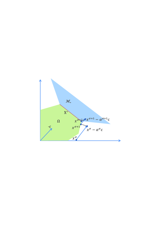
Figure 1: Projected gradient method for LP

Theorem 3.1

$-c\in$ int $\mathcal{M}^{\infty}_{*}$, where $\mathcal{M}^{\infty}_{*}$ is the asymptotic cone of $\mathcal{M}_{*}$ and $\rm{int}~{}\mathcal{M}^{\infty}_{*}$ denotes the interior of $\mathcal{M}^{\infty}_{*}$.

$Proof.$ We know from the optimality conditions that

$$\begin{array}[]{l}-c\in N_{\Omega}(x^{*}),\forall x^{*}\in X^{*}.\end{array}$$

Then we have $x^{*}+t(-c)\in\mathcal{M}_{*}$, $\forall t\geq 0$, which implies

$$\begin{array}[]{l}-c\in\mathcal{M}^{\infty}_{*}.\end{array}$$ (46)

Define

$$\begin{array}[]{l}\mathcal{T}(x^{*},d)=\{t|x^{*}+td\in X^{*}\},\end{array}$$

where $d\in R^{n}$ and satisfies $d^{T}c=0$. Because $X^{*}$ is a closed convex set, $\mathcal{T}(x^{*},d)$ is a closed interval. Next, we prove that

$$\begin{array}[]{l}-c\in\rm ri~{}(\rm{span}\{-\emph{c},\emph{d}\}\cap\mathcal{M}^{\infty}_{*}),\end{array}$$ (47)

where ri $S$ denotes the relative interior of $S$.

If $\mathcal{T}(x^{*},d)=(-\infty,+\infty)$, clearly, $d$, $-d\in\mathcal{M}^{\infty}_{*}$. Therefore, (47) is obvious by (46).

If $\mathcal{T}(x^{*},d)=(-\infty,t_{\max}]$ and $t_{\max}<\infty$. Similar to above, $-d\in\mathcal{M}^{\infty}_{*}$. Moreover, there exists $u\in N_{\Omega}(x^{*}+t_{\max}d)\cap\rm{span}\{-\emph{c},\emph{d}\}$ that satisfies $\langle u,-d\rangle<0$; therefore, (47) holds for $d^{T}c=0$. Moreover, if there exists no such $u$, we can find $t^{{}^{\prime}}_{\max}>t_{\max}$ such that $x^{*}+t^{{}^{\prime}}_{\max}d\in X^{*}$ because $\Omega$ is a convex polyhedron, which contradicts the definition of $\mathcal{T}(x^{*},d)$.

If $\mathcal{T}(x^{*},d)=[t_{\min},+\infty)$ and $t_{\min}>-\infty$. let $\tilde{d}=-d$; then, $\mathcal{T}(x^{*},\tilde{d})=(-\infty,-t_{\min}]$. Therefore, we have $-c\in\rm ri~{}(\rm{span}\{-\emph{c},\tilde{\emph{d}}\}~{}\cap~{}\mathcal{M}^{\infty}_{*})=\rm ri~{}(\rm{span}\{-\emph{c},\emph{d}\}~{}\cap~{}\mathcal{M}^{\infty}_{*})$ from the situation above.

If $\mathcal{T}(x^{*},d)=[t_{\min},t_{\max}]$ and $t_{\min}>-\infty$, $t_{\max}<\infty$, then, similar to above, there exists $u_{1}\in N_{\Omega}(x^{*}+t_{\min}d)~{}\cap~{}\rm{span}\{-\emph{c},\emph{d}\}$ and $u_{2}\in N_{\Omega}(x^{*}+t_{\max}d)~{}\cap~{}\rm{span}\{-\emph{c},\emph{d}\}$ such that

$$\langle u_{1},d\rangle<0~{}\rm and~{}\langle\emph{u}_{2},\emph{d}\rangle>0.$$

Thus, (47) holds for $d^{T}c=0$.

Because $d$ is arbitrary in the space $\{s|s^{T}c=0\}$, we have $-c\in\rm int\hskip 0.85355pt(\mathcal{M}^{\infty}_{*})$ from (47).

Theorem 3.2

For any $x^{0}\in\mathbb{R}^{n}$, assume that the sequence $\{x^{\sigma}\}$ is obtained by $(\ref{pg subproblem})$; then,

1. There exists an $\bar{\alpha}$ such that if $\alpha^{0}\geq\bar{\alpha}$, then $x^{1}\in X^{*}$.

2. There exists $0<\theta_{\min}\leq\frac{\pi}{2}$ such that

   $$\begin{array}[]{l}c^{T}x^{\sigma}-c^{T}x^{\sigma+1}\geq\alpha^{\sigma}(1-\cos\hskip 1.42271pt\theta_{\min})\Arrowvert c\Arrowvert^{2},\end{array}$$

   if $x^{\sigma+1}\notin X^{*}$. Moreover, $\theta_{\min}=\arccos\left(\frac{\Arrowvert P_{\rm bd(\mathcal{M}^{\infty}_{*})}(-c)\Arrowvert}{\Arrowvert c\Arrowvert}\right)$, where $\rm bd(\hskip 0.85355pt\mathcal{M}^{\infty}_{*})$ denotes the boundary of $\mathcal{M}^{\infty}_{*}$, $P_{\rm bd(\mathcal{M}^{\infty}_{*})}(\cdot)$ denotes the projection onto bd$(\mathcal{M}^{\infty}_{*})$.

3. For any $\alpha>0$, $p\in\{-1\cup\mathcal{N}^{+}\}$, if $\alpha^{\sigma}\geq\alpha$, for $\sigma=p,p+1,...$, then there exists $\Gamma=\left[\frac{c^{T}x^{p+1}-c^{T}x^{*}}{\alpha(1-\cos\hskip 1.42271pt\theta_{\min})\Arrowvert c\Arrowvert^{2}}+p+2\right]_{+}$, such that $x^{\Gamma}\in X^{*}$.

$Proof.$ We prove each of the three claims in turn.

(i) Define $B(r)=\{x|\Arrowvert x\Arrowvert\leq r\}$. Because $-c\in$ int $\mathcal{M}^{\infty}_{*}$, there exists $\varepsilon>0$ such that

$$-c+B(\varepsilon)\subset\mathcal{M}^{\infty}_{*}.$$

Then for any $x\in\mathcal{M}_{*}$ and $\alpha>0$, we arrive at

$$x+\alpha B(\varepsilon)-\alpha c=x+\alpha(-c+B(\varepsilon))\subset\mathcal{M}_{*}.$$

Let $\bar{\alpha}=\frac{\Arrowvert x^{0}-x\Arrowvert}{\varepsilon}$; hence,

$$x^{0}-\bar{\alpha}c = x+x^{0}-x-\bar{\alpha}c$$

$$= x+\frac{\Arrowvert x^{0}-x\Arrowvert}{\varepsilon}\cdot\frac{\varepsilon(x^{0}-x)}{\Arrowvert x^{0}-x\Arrowvert}-\bar{\alpha}c$$

$$\subset x+\bar{\alpha}B(\varepsilon)-\bar{\alpha}c$$

$$\subset \mathcal{M}_{*}.$$

Moreover, for any $\alpha\geq\bar{\alpha}$

$$x^{0}-\alpha c = x^{0}-\bar{\alpha}c-(\bar{\alpha}-\alpha)c$$

$$\subset -(\bar{\alpha}-\alpha)c+\mathcal{M}_{*}$$

$$\subset \mathcal{M}_{*}.$$

Thus, from the definition of $\mathcal{M}_{*}$, we have $x^{1}=P_{\Omega}(x^{0}-\alpha^{0}c)\in X^{*}$, $\alpha^{0}\geq\bar{\alpha}$ .

(ii) If $x^{\sigma+1}=x^{\sigma}-\alpha^{\sigma}c$, then

$$c^{T}x^{\sigma}-c^{T}x^{\sigma+1}=\alpha^{\sigma}\Arrowvert c\Arrowvert^{2}.$$

If $x^{\sigma+1}\neq x^{\sigma}-\alpha^{\sigma}c$, then

$$\langle x^{\sigma}-x^{\sigma+1},x^{\sigma}-\alpha^{\sigma}c-x^{\sigma+1}\rangle\geq\frac{\pi}{2}$$

holds by (45), where $\langle s_{1},s_{2}\rangle$ denotes the angle between $s_{1}$ and $s_{2}$. Let $\theta$ denote the angle between $x^{\sigma}-\alpha^{\sigma}c-x^{\sigma+1}$ and $-c$. Because $x^{\sigma+1}\notin X^{*}$, we obtain $x^{\sigma}-\alpha^{\sigma}c-x^{\sigma+1}\notin\rm int\mathcal{M}^{\infty}_{*}$ from the convexity of $\Omega$. Thus, we have $\theta\geq\theta_{\min}=\arccos(\frac{\Arrowvert P_{\rm[bd\mathcal{M}^{\infty}_{*}]}(-c)\Arrowvert}{\Arrowvert c\Arrowvert})$ from $-c\in\rm int\hskip 0.85355pt\mathcal{M}^{\infty}_{*}$. So

$$c^{T}x^{\sigma}-c^{T}x^{\sigma+1} = c^{T}x^{\sigma}-c^{T}P_{[x^{\sigma},x^{\sigma}-\alpha^{\sigma}c]}(x^{\sigma+1})$$

$$= c^{T}x^{\sigma}-c^{T}(x^{\sigma}-\alpha^{\sigma}(1-\cos\hskip 0.85355pt\theta)c)$$

$$\geq \alpha^{\sigma}(1-\cos\hskip 1.42271pt\theta_{\min})\Arrowvert c\Arrowvert^{2},$$

where $[x^{\sigma},x^{\sigma}-\alpha^{\sigma}c]$ denotes a segment whose endpoints are $x^{\sigma}$ and $x^{\sigma}-\alpha^{\sigma}c$. Note that because $-c\in$ int $\mathcal{M}^{\infty}_{*}$, we have $1-\cos\hskip 1.42271pt\theta_{\min}>0$.

(iii) For any $\kappa\geq 1$, if $x^{\sigma}\notin X^{*},~{}\sigma=1,2,..,\kappa$, then we have from (3) that

$$c^{T}x^{p}-c^{T}x^{*} \geq c^{T}x^{p}-c^{T}x^{\kappa}$$

$$= c^{T}x^{p}-c^{T}x^{p+1}+\sum_{\sigma=p+1}^{\kappa-1}(c^{T}x^{\sigma}-c^{T}x^{\sigma+1})$$

$$\geq c^{T}x^{p}-c^{T}x^{p+1}+(\kappa-p-1)\alpha(1-\cos\hskip 1.42271pt\theta_{\min})\Arrowvert c\Arrowvert^{2},$$

which implies

$$\kappa\leq\frac{c^{T}x^{p+1}-c^{T}x^{*}}{\alpha(1-\cos\hskip 1.42271pt\theta_{\min})\Arrowvert c\Arrowvert^{2}}+p+1.$$

Then we have (iii) when

$$\Gamma=\left[\frac{c^{T}x^{p+1}-c^{T}x^{*}}{\alpha(1-\cos\hskip 1.42271pt\theta_{\min})\Arrowvert c\Arrowvert^{2}}+p+2\right]_{+}.$$

Moreover, from (3), we have

$$c^{T}x^{p+1}-c^{T}x^{*} \geq \sum_{\sigma=p+1}^{\kappa-1}\alpha^{\sigma}(1-\cos\hskip 1.42271pt\theta_{\min})\Arrowvert c\Arrowvert^{2}$$

if $x^{\kappa}\notin X^{*}$, which implies

$$\sum_{\sigma=p+1}^{\kappa-1}\alpha^{\sigma}\leq\frac{c^{T}x^{p+1}-c^{T}x^{*}}{(1-\cos\hskip 1.42271pt\theta_{\min})\Arrowvert c\Arrowvert^{2}}.$$

Then we obtain $x^{\kappa}\in X^{*}$ so long as

$$\sum_{\sigma=p+1}^{\kappa-1}\alpha^{\sigma}\geq\frac{c^{T}x^{p+1}-c^{T}x^{*}}{(1-\cos\hskip 1.42271pt\theta_{\min})\Arrowvert c\Arrowvert^{2}}.$$

By Theorem 3.2, we have that if LP problem $(\ref{lp})$ has one finite solution, it can be transformed into a finite number of strictly convex QP problems with projection form similar to $(\ref{pg subproblem})$, which is equivalent to (44). We solve every projection problem by using AL-Hom.

4 Numerical results

In this section, we demonstrate the performance of our algorithms. The numerical experiments were performed on the MATLAB 8.1 programming platform (R2013a) running on a machine with the a Windows 7 operating system, an Intel(R) Core(TM)i7 6700 3.40GHz processor and 32 GB of memory. The QP-solvers and LP-solvers in the other software packages were called by the MATLAB interface.

We tested PAL-Hom for solving randomly generated QPs and QPs from the CUTEr test setbongartz1995cute . We also used PAL-Hom to solve the discrete contact problems of elasticity and QPs from SVMs sra2012optimization that were applied to speech recognition and handwritten digit recognition. Finally, we used PP-AL-Hom to solve randomly generated LPs and LPs from the Netlib test set gay1985electronic .

4.1 Experiments on QPs from synthetic data and CUTEr test set

$\bullet$ Randomly generated QPs. In this part, we randomly generated dense and sparse standard QPs $(\ref{scqp})$ with MATLAB codes as follows.

A=sprandn($m,n,d_{A}$); B=sprandn($q,n,d_{B}$); Q=B${}^{\prime}*$B;

r=$-$B${}^{\prime}*$randn($m$,1); b=$10*$randn($m$,1),

where $d_{A},d_{B}$ denote the density of $A$ and $B$ which are pregiven, $d_{Q}$ denotes the density of $Q$, and “randn” denotes normally random distribution function.

Table 1: Randomly generated QPs

Problem	$m$	$q$	$n$	$d_{A}$	$d_{B}$	$d_{Q}$
QP-D1	800	200	2000	1	1	1
QP-D2	2000	4500	5000	1	1	1
QP-D3	100	5000	10000	1	1	1
QP-D4	4000	9000	10000	1	1	1
QP-S1	10	10	5000	0.01	0.003	9.48E-5
QP-S2	4000	10000	10000	0.01	0.001	1.10E-3
QP-S3	8000	10000	20000	0.001	0.0001	1.49E-4
QP-S4	12000	29999	30000	0.001	0.0001	3.33E-4
QP-S5	1000	4000	50000	0.001	0.0001	1.20E-4
QP-S6	1000	99000	100000	0.001	0.00002	4.39E-5

Table 2: Experiments on randomly generated QPs. $f_{*}$, $f_{S}$ denote the optimal values obtained by PAL-Hom and the other corresponding solvers, “OT” denote the computation times (seconds) more than 25000s. The bolded computation times of PAL-Hom denotes that they are smaller than those of the other solvers.

Problem	Results	PAL-Hom	IPM(cplex)	AS(matlab)	PAS(qpOASES)
m
n
QP-D1	Time	39.30	242.23	10314.69	2342.48
800	$\|Ax-b\|$	1.6E-11	2.9E-06	1.1E-11	1.2E-12
2,000	$f_{*}-f_{S}$	-	-2.2E-06	-1.3E-08	-2.4E-08
QP-D2	Time	35.45	633.12	OT	OT
2,000	$\|Ax-b\|$	6.9E-12	2.8E-07	-	-
5,000	$f_{*}-f_{S}$	-	-7.6E-04	-	-
QP-D3	Time	203.44	5238.28	OT	OT
100	$\|Ax-b\|$	1.7E-11	4.4E-07	-	-
10,000	$f_{*}-f_{S}$	-	-1.2E-03	-	-
QP-D4	Time	369.67	6462.42	OT	OT
4,000	$\|Ax-b\|$	1.2E-07	7.7E-07	-	-
10,000	$f_{*}-f_{S}$	-	-4.9E-03	-	-
QP-S1	Time	0.92	0.14	OT	74.22
10	$\|Ax-b\|$	6.2E-09	8.2E-06	-	5.9E-13
5,000	$f_{*}-f_{S}$	-	-1.3E-09	-	1.3E-04
QP-S2	Time	47.07	126.44	OT	OT
4,000	$\|Ax-b\|$	3.5E-08	1.5E-05	-	-
10,000	$f_{*}-f_{S}$	-	5.7E-07	-	-
QP-S3	Time	208.33	128.72	OT	OT
8,000	$\|Ax-b\|$	8.8E-08	5.8E-07	-	-
20,000	$f_{*}-f_{S}$	-	-1.3E-04	-	-
QP-S4	Time	253.49	5831.07	OT	OT
12,000	$\|Ax-b\|$	3.4E-08	7.9E-07	-	-
30,000	$f_{*}-f_{S}$	-	-2.2E-03	-	-
QP-S5	Time	520.98	1784.71	OT	OT
1,000	$\|Ax-b\|$	1.7E-09	5.2E-08	-	-
50,000	$f_{*}-f_{S}$	-	2.6E-07	-	-
QP-S6	Time	1757.49	4416.68	OT	OT
1,000	$\|Ax-b\|$	1.1E-08	4.4E-04	-	-
100,000	$f_{*}-f_{S}$	-	-2.1E-07	-	-

$\bullet$ QPs from CUTEr set. In this part, we took convex QPs from the CUTEr test set, where we chose a subset of medium-scale QPs having up to 90,597 variables.

Table 3: Experiments on QPs from CUTEr test set: part I. $f_{*}$, $f_{S}$ denote the optimal values obtained by PAL-Hom and the other corresponding solvers, “OT” denotes the computation times (seconds) more than 25000s. “F” denotes that the algorithm does not converges in $10n$ iterations. The bolded computation times of PAL-Hom denotes that they are smaller than those of the other solvers.

Problem	m	n	Results	AL-Hom	IPM(cplex)	AS(matlab)	PAS(qpOASES)
aug2dcqp	10000	20200	Time	0.65	0.41	OT	OT
			$\|Ax-b\|$	8.0E-13	3.9E-13	-	-
			$f_{*}-f_{S}$	-	-1.1E-03	-	-
aug2dqp	10000	20200	Time	0.66	0.31	OT	OT
			$\|Ax-b\|$	9.8E-13	4.2E-13	-	-
			$f_{*}-f_{S}$	-	-1.0E-04	-	-
aug3dcqp	1000	3873	Time	0.14	0.04	569.22	2763.23
			$\|Ax-b\|$	2.4E-14	2.4E-13	2.4E-13	3.0E-15
			$f_{*}-f_{S}$	-	-2.7E-06	-1.4E-09	4.3E-12
aug3dqp	1000	3873	Time	0.20	0.05	OT	3513.54
			$\|Ax-b\|$	1.9E-13	1.1E-14	-	7.4E-11
			$f_{*}-f_{S}$	-	-7.5E-08	-	3.3E-10
cont-050	2401	2597	Time	0.92	0.27	17.92	5397.38
			$\|Ax-b\|$	1.5E-13	3.8E-14	1.2E-13	4.7E-14
			$f_{*}-f_{S}$	-	-7.2E-10	-3.3E-13	2.1E-09
cont-100	9801	10197	Time	2.18	0.56	817.25	OT
			$\|Ax-b\|$	4.0E-13	7.4E-14	1.7E-12	-
			$f_{*}-f_{S}$	-	4.1E-08	-3.3E-13	-
cont-101	10098	10197	Time	4.18	0.84	848.61	OT
			$\|Ax-b\|$	7.3E-13	8.5E-10	3.3E-12	-
			$f_{*}-f_{S}$	-	4.2E-07	-2.4E-06	-
cont-200	39601	40397	Time	11.00	1.40	OT	OT
			$\|Ax-b\|$	5.5E-13	1.5E-13	-	-
			$f_{*}-f_{S}$	-	7.3E-07	-	-
cont-201	40198	40397	Time	23.13	2.31	OT	OT
			$\|Ax-b\|$	7.2E-10	1.8E-08	-	-
			$f_{*}-f_{S}$	-	1.7E-06	-	-
cont-300	90298	90597	Time	41.46	4.62	OT	OT
			$\|Ax-b\|$	8.4E-09	2.8E-08	-	-
			$f_{*}-f_{S}$	-	4.1E-05	-	-
cvxqp1$\_$l	5000	10000	Time	50.22	24.65	OT	OT
			$\|Ax-b\|$	9.9E-08	5.4E-07	-	-
			$f_{*}-f_{S}$	-	-2.5E-02	-	-
cvxqp1$\_$m	500	1000	Time	0.48	0.87	7.61	92.43
			$\|Ax-b\|$	7.2E-13	1.9E-07	8.2E-14	2.5E-13
			$f_{*}-f_{S}$	-	-1.7E-04	1.2E-05	-1.6E-04
cvxqp1$\_$s	50	100	Time	0.01	0.02	0.02	0.15
			$\|Ax-b\|$	2.1E-14	9.5E-12	9.8E-15	2.9E-15
			$f_{*}-f_{S}$	-	-1.5E-05	3.1E-09	-5.2E-07
cvxqp2$\_$l	2500	10000	Time	1.78	12.63	OT	OT
			$\|Ax-b\|$	1.8E-08	1.2E-08	-	-
			$f_{*}-f_{S}$	-	-1.9E-03	-	-
cvxqp2$\_$m	250	1000	Time	0.15	0.53	21.72	26.37
			$\|Ax-b\|$	7.5E-08	3.8E-08	3.8E-14	7.7E-15
			$f_{*}-f_{S}$	-	-1.3E-03	4.3E-06	-3.1E-07
cvxqp2$\_$s	25	100	Time	0.01	0.02	0.04	0.05
			$\|Ax-b\|$	6.8E-08	3.8E-10	8.5E-15	2.6E-15
			$f_{*}-f_{S}$	-	-4.0E-05	-5.0E-08	1.3E-06
cvxqp3$\_$l	7500	10000	Time	54.44	30.19	OT	OT
			$\|Ax-b\|$	4.8E-05	1.9E-05	-	-
			$f_{*}-f_{S}$	-	-6.7E-04	-	-
cvxqp3$\_$m	750	1000	Time	0.66	0.95	10.11	292.15
			$\|Ax-b\|$	7.5E-08	3.6E-09	1.7E-13	4.4E-12
			$f_{*}-f_{S}$	-	-5.6E-02	2.3E-05	1.2E-04
cvxqp3$\_$s	75	100	Time	0.01	0.01	0.03	0.22
			$\|Ax-b\|$	1.8E-09	6.6E-12	1.7E-14	1.9E-14
			$f_{*}-f_{S}$	-	-9.7E-06	2.7E-08	-2.1E-07
gouldqp2	349	699	Time	0.00	0.01	0.11	0.02
			$\|Ax-b\|$	0.0E+00	1.9E-08	0.0E+00	0.0E+00
			$f_{*}-f_{S}$	-	-3.0E-11	0.0E+00	0.0E+00
gouldqp3	349	699	Time	0.04	0.02	0.15	55.74
			$\|Ax-b\|$	1.3E-11	3.8E-09	1.0E-13	1.5E-14
			$f_{*}-f_{S}$	-	-3.1E-06	2.3E-06	-2.1E-10

Table 4: Experiments on QPs from CUTEr test set: part II. $f_{*}$, $f_{S}$ denote the optimal values obtained by PAL-Hom and the other corresponding solvers, “OT” denotes the computation times (seconds) more than 25000s. “F” denotes that the algorithm does not converges in $10n$ iterations. The bolded computation times of PAL-Hom denote that they are smaller than those of the other solvers.

Problem	m	n	Results	PAL-Hom	IPM(cplex)	AS(matlab)	PAS(qpOASES)
powell20	10000	10000	Time	0.14	0.17	OT	OT
			$\|Ax-b\|$	2.5E-08	1.3E-05	-	-
			$f_{*}-f_{S}$	-	3.9E-03	-	-
qgrow7	140	301	Time	0.37	0.01	F	1.56
			$\|Ax-b\|$	2.5E-08	1.0E-10	-	1.6E-02
			$f_{*}-f_{S}$	-	-2.3E-03	-	1.4E-01
qgrow15	300	645	Time	1.55	0.02	F	1936.40
			$\|Ax-b\|$	2.8E-08	2.5E-10	-	1.5E-14
			$f_{*}-f_{S}$	-	-8.6E-03	-	-4.2E-11
qgrow22	440	946	Time	0.57	0.28	F	5924.02
			$\|Ax-b\|$	6.1E-11	4.6E-07	-	4.9E-12
			$f_{*}-f_{S}$	-	7.2E-05	-	-3.3E-09
qscsd1	77	760	Time	0.10	0.02	F	1.44
			$\|Ax-b\|$	4.0E-08	3.7E-11	-	9.1E-10
			$f_{*}-f_{S}$	-	-1.1E-08	-	3.2E-08
qscsd6	147	1350	Time	0.17	0.02	F	11.26
			$\|Ax-b\|$	3.9E-08	2.1E-12	-	9.1E-10
			$f_{*}-f_{S}$	-	-5.1E-08	-	3.3E-09
qscsd8	397	2750	Time	0.89	0.03	F	36.87
			$\|Ax-b\|$	3.0E-08	2.5E-08	-	2.5E-12
			$f_{*}-f_{S}$	-	-1.0E-06	-	3.2E-09
stcqp1	2052	4097	Time	0.13	0.07	1357.24	499.14
			$\|Ax-b\|$	4.0E-09	4.0E-13	4.1E-12	8.1E-13
			$f_{*}-f_{S}$	-	-1.3E-04	3.3E-06	-3.7E-08
stcqp2	2052	4097	Time	0.06	0.67	916.18	1420.90
			$\|Ax-b\|$	3.1E-08	0.0E+00	3.6E-11	3.7E-11
			$f_{*}-f_{S}$	-	-1.1E-04	-3.7E-11	2.2E-08

We compared PAL-Hom with the IPM solver in CPLEX 12.6, the PAS solver in qpOASES and the AS solver in MATLAB 2013a. The comparison includes the computation time (seconds), equality constraint violations and optimal values. The results are reported in Tables 2-4.

The numerical results show that PAL-Hom is effective at solving these QPs. PAL-Hom outperforms the AS solver in MATLAB and the PAS solver in qpOASES and is competitive with the IPM solver in CPLEX, especially for the randomly generated problems.

Moreover, to show that the homotopy algorithm with warm start by APG is meaningful for the augmented Lagrangian subproblems, we compared the algorithm with the IPM solver in CPLEX and Hager et al.’s active-set algorithm (ASA) hager2006new , which consists of a nonmonotone gradient projection step, an unconstrained optimization step, and a set of rules for branching between the two steps. ASA is shown to be faster than TRON lin1999newton for solving the 50 box-constrained problems in the CUTEr library bongartz1995cute and competitive with TRON for the 23 box-constrained problems in the MINPACK-2 library averick1992minpack . Furthermore, to show that the homotopy tracking with the sorting technique and the $\varepsilon$-precision verification and correction technique is more efficient than the PAS solver in qpOASES for solving parametric nonnegative QP problems, we compared it with the PAS solver in qpOASES for solving the first augmented Lagrangian subproblem (8) from $\hat{z}$.

The results are reported in Table 5. Clearly, the homotopy tracking is much faster than the PAS solver in qpOASES. Moreover, from the results, we see that APG is efficient at predicting the optimal active set; that is, from the approximate solution, a small number of tracking steps is required to obtain an exact solution. In addition, we see that the homotopy algorithm is robust for problems with large condition numbers. Simultaneously, the results demonstrate that the homotopy algorithm is clearly faster than PAS(with initial point $\hat{z}$), ASA and IPM for solving the augmented Lagrangian subproblems.

Table 5: IPM(CPLEX), ASA, PAS solver in qpOASES and the homotopy algorithm solving the first augmented Lagrangian problem. “Total” denotes the computation times (seconds) of APG and the homotopy tracking steps together, “Hom-tra.” denotes the computation times of the homotopy tracking steps starting from $\hat{z}$. The computation times of PAS method denote the cost of solving the parametric quadratic programming from $\hat{z}$. “OT” denotes the computation times more than 25000s. $C_{H}$ denotes the condition number of $H$. The bolded computation times (APG+Hom-tra.) in the “Total” column denotes that they are smaller than those of the other solvers, and the bolded computation times in the “Hom-tra.” column denotes that they are smaller than that of the PAS solver.

Problem	n	$C_{H}$	Homotopy				PAS(qpOASES)		ASA	IPM(cplex)
			Total	Hom-tra.	Iter.		Time	Iter.	Time	Time
aug2dcqp	20200	5.2E+06	0.44	0.16	9		221.33	9	1.90	4.24
aug2dqp	20200	8.0E+13	0.43	0.15	8		273.11	10	12.19	4.30
aug3dcqp	3873	8.6E+03	0.06	0.02	2		16.33	2	0.07	2.01
aug3dqp	3873	2.8E+11	0.07	0.02	2		11.44	2	0.12	1.96
cont-50	2597	3.4E+08	0.48	0.11	4		1.61	4	45.57	0.56
cont-100	10197	1.1E+08	0.84	0.21	4		332.13	4	15.50	4.41
cont-101	10197	2.6E+10	2.22	0.62	21		61.21	25	20990.52	4.55
cont-200	40397	1.2E+10	4.46	0.35	5		171.33	8	OT	27.87
cont-201	40397	4.5E+13	12.88	1.77	38		864.77	44	OT	35.45
cont-300	90597	8.0E+10	27.99	4.99	66		OT	OT	OT	316.99
cvxqp1$\_$l	10000	8.8E+13	5.99	1.66	45		277.33	49	406.54	42.11
cvxqp2$\_$l	10000	6.2E+10	0.56	0.13	10		162.11	11	7.10	40.74
cvxqp3$\_$l	10000	6.3E+08	8.33	2.16	25		311.23	29	114.80	46.22
powell20	10000	4.0E+08	0.04	0.01	2		0.10	4	163.58	0.12
qgrow22	946	6.3E+06	0.30	0.03	3		0.16	3	0.03	0.41
qscsd6	1350	3.0E+10	0.11	0.03	33		0.33	37	14459.72	0.75
qscsd8	2740	1.9E+10	0.40	0.15	72		3.27	81	351.74	0.65
stcqp1	4097	1.3E+03	0.04	0.01	2		0.38	2	0.04	1.27
stcqp2	4097	8.2E+02	0.03	0.01	1		5.43	1	0.04	1.72

Moreover, to show the adaptability of PAL-Hom for the degenerate QP problems, we tested the homotopy method on solving highly ill-conditioned non-negative constrained QP problems. We conducted experiments like this for the efficiency of PAL-Hom depends on the solving of the proximal augmented Lagrangian subproblems which are degenerate non-negative constrained QP problems with proximal terms. We generated the non-negative constrained QP problems (8) with MATLAB codes as follows.

$d={\rm zeros}(n,1);~{}d(1:\gamma n)=\frac{L_{\max}}{\gamma n}(1:\gamma n);~{}H=U^{\prime}*{\rm diag}(d)*U+\delta*I$;

$f={\rm randn}(n,1)$;

where $0<\gamma<1$ denotes the ratio of nonzero eigen-values, $U$ is the unitary matrix.

We generated the problems with $n=2000,L_{\max}=10^{8}$ and $\gamma\in\{0.1,0.5\}$. We adjusted the condition number of $H$ which equals to $\frac{L_{\max}+\delta}{\delta}$ by changing the value of $\delta$. $H$ has $\gamma n$ egien-values bigger than $\delta$ and the rest eigen-values are $\delta$. Obviously, $H$ is ill-conditioned when $\delta$ is small.

We solved these problems by the homotopy algorithm and the active-set method, respectively. The maximum iterations of the active-set method is set to $100*\gamma*n$. The results are shown in Figure 2.

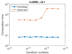
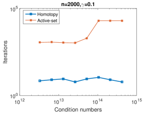
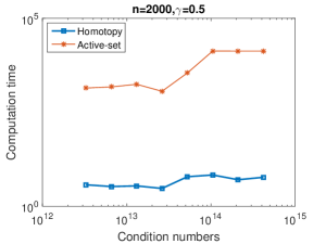
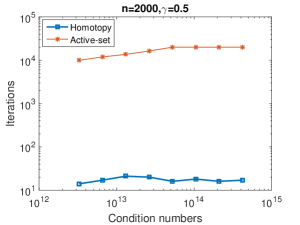
Figure 2: The homotopy and the active-set method for ill-conditioned non-negative constrained QP problems. The results include the computation time (seconds) and the number of the iterations.

The results demonstrate that the homotopy method is robust for the ill-conditioned non-negative constrained QP problems, while the active-set method requires much more time when the condition number is larger. Moreover, the number of steps of the homotopy tracking does not change much when the condition number increases, while the AS method often exceed the maximum iterations when the condition number is very large.

4.2 QPs from SVM for recognition.

In this section, we tested AL-Hom for solving QPs from SVMs that were applied to handwritten digit recognition and speech recognition. Given the training set $\{X_{i},y_{i}\}_{i=1}^{n}$ and testing set $\{T_{j},s_{j}\}_{j=1}^{n_{1}}$, where $X_{i},T_{j}$ are feature vectors and $y_{i},s_{j}\in\{-1,+1\}$ are the labels, the SVM classifies the testing set by a classifier

$$f(x)={\rm sign}(\sum_{i=1}^{n}y_{i}\alpha_{i}^{*}K(X_{i},x)+b^{*}),$$

where $K$ is called the kernel function, $b^{*}=y_{j}-\sum_{i=1}^{n}y_{i}\alpha_{i}^{*}K(X_{i},X_{j})$, for some $\alpha_{j}^{*}>0$, and $\alpha^{*}$ is the solution of the following problem

$$\min_{\alpha}~{}~{}~{}~{}\frac{1}{2}\sum_{i=1}^{n}\sum_{i=1}^{n}y_{i}y_{j}\alpha_{i}\alpha_{j}K(X_{i},X_{j})-\sum_{i=1}^{n}\alpha_{i}$$

$${\rm s.t.}~{}~{}~{}~{}\sum_{i=1}^{n}y_{i}\alpha_{i}=0,$$ (50)

$$~{}~{}~{}~{}~{}~{}~{}~{}~{}0\leq\alpha_{i}\leq C,i=1,...,n,$$

which is a dense QP problem.

We conducted the experiments with three databases. The first database is the isolated letter speech database from UCILichman2013 , which contains a training set with 6,238 samples and a testing set with 1,559 samples. This database has 26 classifications: i.e., A-Z, and every sample has 617 attributes. The second one is the MNIST database of handwritten digits, which contains a training set with 60,000 samples and a testing set with 10,000 samples. Every sample is one $28\times 28$ pixel picture, that is, every sample has 784 attributes. This database has ten classifications as shown in Figure 3. The third database is the web page classification task, which is included in the LIBSVM database set. This database contains 8 training sets and 8 testing sets of different sizes. Every set contains samples divided into 2 classes and every sample has 300 features. Because the training sets have repetitive samples, we processed them individually by removing the repetitive samples.

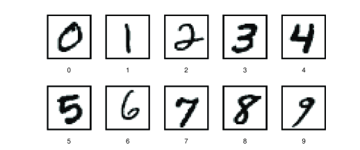
Figure 3: Ten classifications of the MNIST handwritten digit database

(50) is a model for the 2-class classification problem; however, the letter speech and MNIST databases are multiclassification problems. Therefore. we handled the multiclassification problems with two strategies.

The first strategy is that for any classification $p,p=1,..,P$, where $P$ denotes the number of classifications, we obtained $\alpha^{*,p},b^{*,p}$ by solving (50) with

$$y^{p}=\left\{\begin{array}[]{lcl}1,&&X_{i}\in cl.p;\\ -1,&&else,\end{array}\right.$$ (53)

where $cl.p$ denotes the $p$-th classification. Then, we have the first classifier for multiclassification problems as follows

$$f_{1}(x)=\arg\max_{p}~{}(y^{p}_{i}\alpha_{i}^{*,p}K(X_{i},x)+b^{*,p}).$$ (54)

The second strategy is that for any $p\neq q\in\{1,...,P\}$, choose the samples from the training set whose corresponding labels are $p$ or $q$, and let

$$y^{p,q}=\left\{\begin{array}[]{lcl}1,&&X_{i}\in cl.p;\\ -1,&&X_{i}\in cl.q,\end{array}\right.$$

then, we have the second classifier for multiclassification problems as follows.

$$f_{2}(x)=\arg\max_{p}~{}\sum_{q}{\rm sign}(y^{p,q}_{i}\alpha_{i}^{*,p,q}K(X_{i},x)+b^{*,p,q}).$$ (55)

The first strategy needs to solve $(\ref{svm})$ $P$ times, and the size of every problem is equal to the number of samples in the training set. The second strategy needs to solve $(\ref{svm})$ $\frac{P(P-1)}{2}$ times, however, it only needs to solve a problem of size equal to the number of samples of the classification $p$ and $q$ together each time. In LIBSVM, the multiclassification classifier adopts the second strategy.

In our experiments, we used the polynomial kernel

$$K(x,y)=(x\cdot y+c)^{d}$$

with $c=0$ and $d=2$ for the spoken letter database and the MNIST databases and the Gaussian kernel

$$K(x,y)=e^{-\sigma\|x-y\|^{2}}$$

with $\sigma=0.1$ for the web pages classification task.

Because the QP problems in this section are strictly convex, we compared AL-Hom with the IPM solver in CPLEX and the sequential minimal optimization (SMO) method fan2005working in LIBSVM 3.22 CC01a which is a well-known package for SVMs. We report the results in Tables 6 and 7, where “Err.1” and “Err.2”, respectively, denote the number of misclassifications of classifier $(\ref{classifier})$ and classifier $(\ref{classifier2})$ for the test set. Here, we simply list the computation time of the first strategy and not that of the second strategy because it contains $\frac{P(P-1)}{2}$ parts. We only give the total time of the second strategy in the title of the tables. Moreover, we do not list the results of IPM for the MNIST database because it took substantially more time than the other two algorithms. The results show that the IPM solver in CPLEX faces difficulties in solving the QPs from SVMs. PAL-Hom outperforms IPM. Moreover, although AL-Hom does not exploit the structure or particularity, it is competitive with SMO which extensively exploits the structure and particularity of the SVM problem. We believe that AL-Hom would be more competitive for SVMs if we implement AL-Hom using the structure and the particularity the SVM problem, such as utilizing the framework of Osuna’s decomposition algorithm osuna1997improved .

Table 6: Experiments on QPs from SVM for the classification of the isolated letter speech database. The computation time (seconds) in this table is the cost of the first strategy. In the second strategy, AL-Hom took 4.92s, IPM took 107.08s and SMO took 13.37s in all. The bolded computation times of AL-Hom denotes that they are smaller than those of the other solvers.

Class.	AL-Hom				IPM (cplex)				SMO (LIBSVM)
	Time/s	Err.1	Err.2		Time/s	Err.1	Err.2		Time/s	Err.1	Err.2
cl.A	3.43	0	0		240.80	0	0		6.65	0	0
cl.B	4.33	5	4		242.58	5	4		7.23	5	4
cl.C	1.77	0	0		259.33	0	0		5.22	0	0
cl.D	5.01	4	3		233.34	4	3		6.86	4	3
cl.E	3.10	0	2		255.32	0	2		6.77	0	2
cl.F	3.16	0	2		232.10	0	2		6.84	0	2
cl.G	3.95	0	0		260.34	0	0		6.98	0	0
cl.H	1.88	0	0		220.50	0	0		4.82	0	0
cl.I	1.84	1	1		223.03	1	1		5.37	1	1
cl.J	1.80	1	1		273.58	1	1		6.45	1	1
cl.K	3.87	2	2		218.09	2	2		6.94	1	2
cl.L	1.74	0	0		200.01	0	0		5.33	0	0
cl.M	3.66	9	7		252.48	9	6		5.34	9	6
cl.N	4.32	8	9		230.56	8	9		6.73	8	9
cl.O	3.20	0	0		208.38	0	0		7.28	0	0
cl.P	6.73	0	6		235.25	0	5		5.41	0	5
cl.Q	1.71	4	0		226.73	4	0		7.78	4	0
cl.R	1.44	0	0		258.80	0	0		5.22	0	0
cl.S	1.54	3	3		229.37	3	3		4.94	3	3
cl.T	4.63	3	5		231.48	3	6		7.30	3	6
cl.U	1.90	2	2		225.77	2	2		5.88	2	2
cl.V	5.33	5	6		231.16	5	5		7.02	5	5
cl.W	2.38	0	0		256.07	0	1		6.57	0	1
cl.X	1.63	0	0		228.58	0	0		5.02	0	0
cl.Y	1.44	0	0		220.33	0	0		4.49	0	0
cl.Z	2.13	4	3		247.07	4	3		5.91	4	3
Total	77.93	51	56		6138.86	51	55		161.59	51	55

Table 7: Experiments on QPs from SVM for the classification of the mnist database. The computation time (seconds) in this table is the cost of the first strategy. In the second strategy, AL-Hom took 394.33s and SMO took 282.43s in all. The bolded computation times of AL-Hom denotes that they are smaller than those of the other solvers.

Class.	AL-Hom				SMO (LIBSVM)
	Time/s	Err.1	Err.2		Time/s	Err.1	Err.2
cl.0	901.33	10	7		939.29	10	8
cl.1	644.27	10	7		540.36	10	8
cl.2	2001.13	22	24		2336.39	22	24
cl.3	2225.65	23	23		3501.45	23	25
cl.4	2001.42	17	16		1492.39	17	16
cl.5	1978.43	19	20		2397.18	19	19
cl.6	1117.33	17	18		1057.11	17	18
cl.7	1863.33	22	25		1926.60	22	26
cl.8	2854.22	24	22		4028.26	24	23
cl.9	2131.33	29	30		4111.90	29	28
Total.	17718.44	193	192		22230.8	193	195

Table 8: Experiments on QPs from SVM for the classification of the web classification task. “OT” denotes the computation times more than 25000s.

Problem	Training.set	Testing.set	AL-Hom			IPM (cplex)			SMO (LIBSVM)
			Time/s	Err.		Time/s	Err.		Time/s	Err.
w1a	2123	47272	0.93	1030		6.40	1030		0.40	1030
w2a	2950	46279	1.37	895		18.01	895		0.64	895
w3a	4108	44837	2.65	823		54.81	823		1.02	823
w4a	6049	42383	5.34	728		205.78	728		1.88	728
w5a	7970	39861	11.22	648		620.39	648		3.02	648
w6a	13268	32561	34.78	419		2950.54	419		7.14	419
w7a	18530	25057	103.13	321		8766.35	321		25.64	321
w8a	34704	14951	553.74	113		OT	-		165.54	113

AL-Hom is much faster than IPM implemented in CPLEX for solving QPs from SVMs for the following two reasons: first, ALM is effective for SVM optimization because it requires only several iterations to achieve a satisfactory solution; second, from (26)-(27), we know that the homotopy algorithm needs to solve two linear systems of size $|J^{i}|$ at each step. Because the number of support vectors is often small, that is, $\alpha^{*}$ is sparse, the homotopy algorithm solves smaller scale linear systems than IPM. This good property of $\alpha^{*}$ makes AL-Hom perform well in solving SVM optimizations.

4.3 Contact problems of elasticity

In this section, we solve the contact problems of elasticity used as a benchmark in dostal2000solution ; dostal2000duality ; dostal2003augmented

$$\begin{array}[]{l}{\rm Minimize}~{}~{}~{}q(u_{1},u_{2})=\sum_{i=1}^{2}\left(\int_{\Omega_{i}}|\nabla u_{i}|^{2}d\Omega-\int_{\Omega_{i}}Pu_{i}d\Omega\right),\\ {\rm subject~{}to}~{}~{}~{}u_{1}(0,y)=0~{}{\rm and}~{}u_{1}(1,y)\leq u_{2}(1,y)~{}{\rm for}~{}y\in[0,1],\end{array}$$ (56)

where $\Omega_{1}=(0,1)\times(0,1)$, $\Omega_{2}=(1,2)\times(0,1)$, $P(x,y)=-5$ for $(x,y)\in(0,1)\times[0.75,1)$, $P(x,y)=0$ for $(x,y)\in(0,1)\times(0,0.75)$, $P(x,y)=-1$ for $(x,y)\in(1,2)\times(0,0.25)$ and $P(x,y)=0$ for $(x,y)\in(1,2)\times(0.25,1)$.

We followed Dostál et al. using finite difference to discretize (56) by regular grids that are defined by the step size $h\in\{\frac{1}{32},\frac{1}{64},\frac{1}{128},\frac{1}{256},\frac{1}{512},\frac{1}{1024}\}$ in each direction in each subdomain $\Omega_{i}$.

The discrete problem is a QP problem

$$\begin{array}[]{l}\min~{}~{}\frac{1}{2}x^{T}Qx+r^{T}x\\ \rm{s.t.}~{}~{}~{}\emph{Ax}\leq 0,\end{array}$$ (57)

which is transformed to form (1) by introducing a slack variable $s$

$$\begin{array}[]{l}\min~{}~{}\frac{1}{2}x^{T}Qx+r^{T}x\\ \rm{s.t.}~{}~{}~{}\emph{Ax}+s=0\\ ~{}~{}~{}~{}~{}~{}~{}s\geq 0.\end{array}$$ (58)

Thus, when $h=\frac{1}{1024}$, (58) has 2,101,250 variables and 1,025 equality constraints. We used PAL-Hom to solve (58) and compare it with the IPM solver in CPLEX. Moreover, to show that the strategy which uses the homotopy method to obtain the exact solutions of the augmented Lagrangian subproblems is valid, we also exactly asymptotically solved the augmented Lagrangian subproblems by the APG method. For convenience, we use PAL-APG to denote the augmented Lagrangian iterations with the subproblems exactly asymptotically solved by APG.

Table 9: Experiments on the discrete contact problems of elasticity, “Iter” denotes the number of the augmented Lagrangian subproblems solved. “Total” denotes the computation time (seconds) of APG and the homotopy tracking steps together (for all augmented Lagrangian subproblems), “Hom-tra.” denotes the computation time of the homotopy tracking steps. “OM” denotes out of memory. The bolded computation times of PAL-Hom denotes that they are smaller than those of the other solvers.

$h$	$m$	$n$	PAL-Hom				PAL-APG			IPM(cplex)
			Iter	Total	Hom-tra.		Iter	Time
$1/32$	33	2,178	5	0.09	0.02		11	1.33		0.32
$1/64$	65	8,450	5	0.32	0.06		11	3.34		1.34
$1/128$	129	33,282	5	1.09	0.18		12	17.45		13.33
$1/256$	257	132,098	6	12.28	0.85		11	324.49		127.42
$1/512$	513	526,338	6	129.14	10.09		11	1651.90		1408.52
$1/1024$	1,025	2,101,250	6	873.17	67.33		12	12937.68		OM

From the results, we see that PAL-Hom requires fewer iterations than PAL-APG. Moreover the computation time of PAL-Hom is substantially smaller than that of PAL-APG. Furthermore, when the APG iteration obtains a low-precision solution, a good prediction of the optimal active set is obtained; therefore, the homotopy algorithm requires a small number of steps and little time to obtain the exact solution from the approximate solution. However, APG must continue iterating for the required precision, which requires much more time. The results demonstrate that exactly solving the subproblems at the mid to end stage by the homotopy algorithm is actually valid and that PAL-Hom is substantially more efficient than IPM for solving this problem.

4.4 Randomly generated LPs and LPs from Netlib test set

In this section, we solve LPs by PP-AL-Hom. We first randomly generated LPs with MATLAB codes as follows.

A=sprandn($m,n,d_{A}$); b=10$*$randn($m$,1); c=rand($n$,1).

Table 10: Randomly generated LP

Problem	$m$	$n$	$d_{A}$
LP-D1	400	1000	1
LP-D2	800	2000	1
LP-D3	1000	5000	1
LP-D4	300	8000	1
LP-D5	4000	10000	1
LP-S1	100	2000	0.01
LP-S2	1000	5000	0.01
LP-S3	800	8000	0.01
LP-S4	4000	10000	0.01
LP-S5	800	15000	0.01
LP-S6	8000	20000	0.001
LP-S7	15000	32000	0.001

Additionally, we chose LPs from the Netlib test set. The chosen LPs have finite solutions and were up to a size $16558\times 49932$. For randomly generated LPs, PAL-Hom started from the original point, and for LPs from the Netlib test set, we used a projected Newton barrier method gill1986projected to obtain an approximate solution as an initial point, which would reduce the number of the iterations (45).

Table 11: Experiments on randomly generated LP. $f_{*}$, $f_{S}$ denote the optimal values obtained by PAL-Hom and the other corresponding solvers, “OT” denote the computation time (seconds) more than 25000s. The bolded computation times of PAL-Hom denotes that they are smaller than those of the other solvers.

Problem	Results	PP-AL-Hom	IPM(cplex)	Simplex(gurobi)	IPM(matlab)	Simplex(matlab)
LP-D1	Time	0.69	0.80	0.58	3.33	17.90
	$\|Ax-b\|$	7.8E-11	4.0E-12	4.8E-12	1.3E-09	6.3E-10
	$f_{*}-f_{S}$	-	-2.1E-11	-2.0E-11	-1.3E-10	-1.2E-11
LP-D2	Time	9.13	8.47	5.59	30.25	232.99
	$\|Ax-b\|$	2.4E-11	1.2E-11	1.3E-11	8.8E-13	3.8E-09
	$f_{*}-f_{S}$	-	-5.3E-12	-6.1E-12	-8.2E-12	1.0E-10
LP-D3	Time	21.90	33.11	16.58	110.67	918.04
	$\|Ax-b\|$	8.9E-10	1.2E-11	1.5E-11	9.9E-13	2.5E-09
	$f_{*}-f_{S}$	-	1.0E-12	1.1E-12	9.9E-13	-1.0E-11
LP-D4	Time	11.36	3.82	2.27	19.47	55.78
	$\|Ax-b\|$	5.7E-10	1.8E-12	1.6E-12	7.5E-11	3.8E-09
	$f_{*}-f_{S}$	-	-6.2E-13	-6.2E-12	-5.0E-12	6.1E-12
LP-D5	Time	343.23	1277.07	460.83	3472.62	OT
	$\|Ax-b\|$	2.2E-10	2.3E-10	2.6E-10	4.0E-12	-
	$f_{*}-f_{S}$	-	-5.0E-12	-1.2E-11	-7.7E-12	-
LP-S1	Time	0.09	0.00	0.00	0.02	0.07
	$\|Ax-b\|$	2.1E-11	1.3E-13	9.7E-14	7.8E-13	4.9E-13
	$f_{*}-f_{S}$	-	-2.1E-14	-2.1E-14	-2.1E-14	-2.3E-14
LP-S2	Time	2.43	1.62	0.93	6.40	350.84
	$\|Ax-b\|$	1.0E-08	1.5E-10	4.5E-11	1.6E-08	2.7E-11
	$f_{*}-f_{S}$	-	-8.1E-10	-8.1E-10	-1.4E-09	-5.3E-09
LP-S3	Time	5.16	1.09	0.39	3.37	171.34
	$\|Ax-b\|$	8.0E-10	2.6E-10	6.8E-12	1.4E-10	2.7E-12
	$f_{*}-f_{S}$	-	-5.3E-09	-5.3E09	-5.4E-10	-5.3E-10
LP-S4	Time	49.37	96.59	59.78	458.33	OT
	$\|Ax-b\|$	4.2E-10	3.8E-09	2.9E-10	6.2E-09	-
	$f_{*}-f_{S}$	-	-5.2E-10	-4.9E-10	1.5E-10	-
LP-S5	Time	5.13	0.48	0.40	4.33	225.65
	$\|Ax-b\|$	6.9E-11	6.2E-11	7.4E-12	4.2E-11	1.9E-10
	$f_{*}-f_{S}$	-	4.2E-12	1.7E-13	3.7E-13	-4.3E-13
LP-S6	Time	311.45	148.93	97.58	3007.46	OT
	$\|Ax-b\|$	6.2E-09	2.7E-08	5.5E-09	1.4E-11	-
	$f_{*}-f_{S}$	-	-2.8E-08	-7.7E-09	-1.8E-09	-
LP-S7	Time	903.11	2024.15	1289.04	24726.41	OT
	$\|Ax-b\|$	2.6E-09	2.1E-07	1.6E-08	1.6E-11	-
	$f_{*}-f_{S}$	-	-1.1E-06	-1.2E-06	-1.3E-06	-

Table 12: Experiments on LPs from Netlib test set: part I (seconds). $f_{*}$, $f_{S}$ denote the optimal values obtained by PAL-Hom and the other corresponding solvers.

Problem	m	n	Results	PP-AL-Hom	cplex	gurobi	matlab
					IPM	Simplex	IPM	Simplex
adlittle	57	138	Time	0.39	0.01	0.00	0.01	0.04
			$\|Ax-b\|$	8.8E-11	2.4E-13	8.1E-14	3.1E-11	3.7E-13
			$f_{*}-f_{S}$	-	-1.4E-08	-1.2E-08	-1.2E-08	-1.2E-08
afiro	27	51	Time	0.04	0.00	0.00	0.01	0.01
			$\|Ax-b\|$	1.4E-13	1.4E-14	1.4E-14	1.5E-12	1.1E-13
			$f_{*}-f_{S}$	-	1.1E-13	01.1E-13	0.0E+00	1.1E-13
agg2	516	758	Time	0.51	0.01	0.01	0.08	1.27
			$\|Ax-b\|$	1.8E-08	1.3E-13	3.4E-10	5.4E-10	1.3E-10
			$f_{*}-f_{S}$	-	-6.9E-04	-6.9E-04	-6.9E-04	-6.9E-04
beaconfd	173	295	Time	0.27	0.00	0.00	0.02	0.02
			$\|Ax-b\|$	4.3E-09	4.1E-11	1.2E-11	5.1E-11	3.2E-11
			$f_{*}-f_{S}$	-	2.3E-04	2.3E-04	2.3E-04	2.3E-04
blend	74	114	Time	0.09	0.00	0.00	0.01	0.03
			$\|Ax-b\|$	2.2E-09	63.9E-14	3.7E-13	6.0E-12	3.9E-14
			$f_{*}-f_{S}$	-	-3.2E-07	-3.2E-07	-3.2E-07	-3.2E-07
d6cube	415	6184	Time	49.13	0.08	0.07	0.40	16.93
			$\|Ax-b\|$	8.6E-09	4.3E-11	7.8E-12	1.9E-09	5.1E-11
			$f_{*}-f_{S}$	-	4.22E-07	4.22E-07	4.22E-07	4.22E-07
degen2	444	754	Time	0.68	0.02	0.02	0.04	2.04
			$\|Ax-b\|$	1.6E-09	3.6E-15	3.6E-15	1.2E-12	2.6E-14
			$f_{*}-f_{S}$	-3.7E-06	-3.7E-06	-3.7E-06	-3.7E-06	-3.7E-06
degen3	1503	2604	Time	17.19	0.31	0.10	0.79	59.33
			$\|Ax-b\|$	6.8E-09	1.1E-14	1.5E-14	7.2E-09	1.1E-13
			$f_{*}-f_{S}$	-	-1.88E-05	-1.88E-05	-1.88E-05	-1.88E-05
maros-r7	3136	9408	Time	2.85	0.46	0.25	3.99	51.18
			$\|Ax-b\|$	8.7E-09	4.6E-09	4.7E-09	1.8E-10	7.7E-08
			$f_{*}-f_{S}$	-	-8.1E-08	-8.2E-08	-8.3E-08	-8.4E-08
psd$\_$02	2953	7716	Time	5.91	0.03	0.02	0.18	2.15
			$\|Ax-b\|$	7.4E-10	0.0E+00	0.0E+00	0.0E+00	0.0E+00
			$f_{*}-f_{S}$	-	0.0E+00	0.0E+00	0.0E+00	0.0E+00
psd$\_$06	9881	29351	Time	26.44	0.16	0.12	6.41	17.81
			$\|Ax-b\|$	6.7E-09	0.0E+00	0.0E+00	0.0E+00	0.0E+00
			$f_{*}-f_{S}$	-	-9.0E-04	-9.0E-04	-9.0E-04	-9.0E-04
psd$\_$10	16558	49932	Time	213.32	0.39	0.21	31.66	50.83
			$\|Ax-b\|$	2.0E-10	0.0E+00	0.0E+00	0.0E+00	0.0E+00
			$f_{*}-f_{S}$	-	-2.8E-03	-2.8E-03	-2.8E-03	-2.8E-03
qap8	912	1632	Time	1.16	0.22	0.46	0.73	15.11
			$\|Ax-b\|$	1.3E-09	5.0E-13	1.7E-12	1.1E-14	2.3E-14
			$f_{*}-f_{S}$	-	3.3E-09	3.3E-09	3.7E-09	9.3E-09
qap12	3192	8856	Time	77.71	1.64	1.10	1506.63	1342.79
			$\|Ax-b\|$	8.6E-10	2.6E-12	1.9E-12	7.9E-09	1.9E-12
			$f_{*}-f_{S}$	-	4.1E-06	4.1E-06	3.9E-06	4.1E-06
scorpion	388	466	Time	0.54	0.01	0.01	0.02	0.22
			$\|Ax-b\|$	3.1E-13	1.2E-15	8.1E-16	2.6E-15	1.2E-15
			$f_{*}-f_{S}$	-	-5.8E-05	-5.8E-05	-5.8E-05	-5.8E-05
scsd1	77	760	Time	0.32	0.01	0.01	0.01	0.09
			$\|Ax-b\|$	9.1E-13	1.5E-16	1.1e-16	2.2e-13	2.1e-16
			$f_{*}-f_{S}$	-	1.6E-11	1.6E-11	-2.5E-10	1.6E-11
scsd6	147	1350	Time	0.29	0.01	0.02	0.02	0.28
			$\|Ax-b\|$	1.9E-12	5.9E-16	3.7E-16	1.9E-13	6.0E-16
			$f_{*}-f_{S}$	-	-1.1E-09	-1.1E-09	-9.0E-09	2.4E-09
scsd8	397	2750	Time	0.19	0.02	0.04	0.02	0.78
			$\|Ax-b\|$	5.9E-11	3.2E-14	3.1E-13	3.1E-13	4.2E-14
			$f_{*}-f_{S}$	-	-1.2E-08	1.5E-08	1.5E-08	1.5E-08
sctap1	300	660	Time	2.31	0.01	0.01	0.03	0.34
			$\|Ax-b\|$	4.7E-10	5.5E-15	2.5E-15	6.0E-11	1.2E-11
			$f_{*}-f_{S}$	-	1.9E-07	1.9E-07	1.9E-07	1.9E-07
sctap2	1090	2500	Time	2.13	0.01	0.02	0.06	5.10
			$\|Ax-b\|$	7.3E-10	1.6E-14	8.9E-16	1.6E-12	3.3E-13
			$f_{*}-f_{S}$	-	-2.5E-07	-2.5E-07	-2.5E-07	-2.5E-07
sctap3	1480	3340	Time	2.32	0.03	0.02	0.06	6.86
			$\|Ax-b\|$	1.2E-09	8.9E-15	6.2E-15	3.2E-12	3.2E-13
			$f_{*}-f_{S}$	-	-6.5E-07	-6.5E-07	-6.5E-07	-6.5E-07

Table 13: Experiments on LPs from Netlib test set: part II (seconds). $f_{*}$, $f_{S}$ denote the optimal values obtained by PAL-Hom and the other corresponding solvers.

Problem	m	n	Results	PP-AL-Hom	cplex	gurobi	matlab
					IPM	Simplex	IPM	Simplex
ship04l	402	2166	Time	0.41	0.01	0.01	0.02	0.25
			$\|Ax-b\|$	3.5E-10	4.4E-14	4.9E-13	4.4E-11	2.3E-14
			$f_{*}-f_{S}$	-	-7.5E-05	-3.1E-05	-3.1E-05	-3.1E-05
ship04s	402	1506	Time	0.30	0.01	0.01	0.02	0.09
			$\|Ax-b\|$	1.7E-09	7.7E-14	2.9E-14	6.8E-09	6.6E-14
			$f_{*}-f_{S}$	-	-4.2E-04	-4.2E-04	-4.2E-04	-4.2E-04
ship08l	778	4363	Time	3.38	0.01	0.01	0.05	0.45
			$\|Ax-b\|$	2.3E-12	4.7E-14	3.2E-14	2.2E-10	1.7E-13
			$f_{*}-f_{S}$	-	-6.5E-07	-1.4E-07	-1.4E-07	-1.4E-07
ship08s	778	2476	Time	2.13	0.02	0.01	0.03	0.18
			$\|Ax-b\|$	1.9E-12	2.8E-14	1.8E-14	2.8E-11	1.0E-11
			$f_{*}-f_{S}$	-3.6E-08	1.1E-07	1.1E-07	1.1E-07	1.1E-07
ship12l	1151	5533	Time	6.33	0.02	0.02	0.06	0.67
			$\|Ax-b\|$	4.4E-12	3.6E-14	3.8E-14	3.3E-11	3.6E-13
			$f_{*}-f_{S}$	-	-2.2E-07	-1.8E-07	-1.8E-07	-1.8E-07
mship12s	1151	2869	Time	2.64	0.01	0.02	0.02	0.28
			$\|Ax-b\|$	1.8E-11	4.9E-13	6.3E-14	3.2E-11	1.1E-13
			$f_{*}-f_{S}$	-	-1.3E-05	-9.5E-07	-9.5E-07	-9.5E-07
truss	1000	8806	Time	2.67	0.07	1.91	0.18	21.66
			$\|Ax-b\|$	1.7E-09	2.1E-13	1.9E-13	1.8E-11	1.0E-11
			$f_{*}-f_{S}$	-	7.2E-06	7.2E-06	7.2E-06	7.2E-06

We report the results in Tables 11-13 and the time of PAL-Hom in Tables 12-13 has included the computation time of the projected Newton barrier method. The results show that PAL-Hom is able to solve the randomly generated LPs and LPs from the Netlib test set. For randomly generated LPs, PAL-Hom is competitive with the other solvers. For LPs from the Netlib test set, PAL-Hom is not as good as the IPM solvers in CPLEX and MATLAB, and the simplex solver in Gurobi, but for some problems, PAL-Hom is more effective than the simplex solver in MATLAB.

5 Conclusion

In this paper, we present a PAL-Hom (AL-Hom) algorithm for convex QP problems, which takes the proximal ALM as the outer iteration and the homotopy algorithm as the inner iteration. Compared with IPM, AS and PAS, the size of the KKT systems solved in PAL-Hom is much smaller, especially when the solution is sparse such as in the problems from SVM. Moreover, compared with PAS, the KKT systems in the tracking steps of PAL-Hom would always be invertible so that we do not need to exchange indices to keep the invertibility as in qpOASES. Furthermore, it is substantially easier to design an efficient warm start for PAL-Hom than for the QP problem (1) (PAS). Although we do not pay significant attention to optimizing the codes, PAL-Hom is shown to be faster than the IPM solver in CPLEX for certain problems, such as randomly generated QPs, LPs and some QPs in the CUTEr test. In particular, SVM problems and the discrete contact problems of elasticity, PAL-Hom is more than 10 times faster than IPM. Given this practical performance, we believe that our algorithms are promising.

The presented homotopy algorithm is shown to be efficient for nonnegative QP problems (augmented Lagrangian subproblems) for the following reasons. First, APG is effective at predicting the optimal active set, which provides a good warm start for the homotopy algorithm. With the warm start, the homotopy algorithm often needs fewer iterations to obtain an exact solution. The Cholesky factor update technique improves the performance of the homotopy algorithm by reducing the computation of solving the KKT systems. Moreover, benefiting from the $\varepsilon$-precision verification and correction technique that address the incorrect update of the active set caused by large condition numbers and a lack of strict complementarity, the homotopy algorithm is shown to be robust for the augmented Lagrangian problems with large condition numbers. The numerical results demonstrate that the homotopy algorithm is substantially more efficient than PAS, ASA and IPM in solving the augmented Lagrangian subproblems.

Simultaneously, based on the AL-Hom method, we use PP-AL-Hom to solve the LP which is proved to converge in a finite number of steps. Moreover, the estimate of the number of maximum iterations and the descent of the objective are presented. The numerical results show that PP-AL-Hom is competitive to IPM in solving randomly generated problems.

References

- (1) Averick, B.M., Carter, R.G., Xue, G.L., Moré, J.J.: The minpack-2 test problem collection. Tech. rep., Argonne National Lab., IL (United States) (1992)
- (2) Bertsekas, D.P.: Nonlinear programming. Athena scientific Belmont (1999)
- (3) Best, M.J.: An algorithm for the solution of the parametric quadratic programming problem. CORR 82-14, Department of Combinatorics and Optimization, University of Waterloo, Canada (1982)
- (4) Best, M.J.: An algorithm for the solution of the parametric quadratic programming problem. Springer (1996)
- (5) Bongartz, I., Conn, A.R., Gould, N., Toint, P.L.: Cute: Constrained and unconstrained testing environment. ACM Transactions on Mathematical Software (TOMS) 21(1), 123–160 (1995)
- (6) Buys, J.D.: Dual algorithms for constrained optimization problems. Brondder-Offset NV-Rotterdam (1972)
- (7) Chang, C.C., Lin, C.J.: LIBSVM: A library for support vector machines. ACM Transactions on Intelligent Systems and Technology 2, 27:1–27:27 (2011). Software available at http://www.csie.ntu.edu.tw/~cjlin/libsvm
- (8) Conn, A.R., Gould, N.I.M., Toint, P.L.: A globally convergent augmented Lagrangian algorithm for optimization with general constraints and simple bounds. SIAM Journal on Numerical Analysis 28(2), 545–572 (1991)
- (9) Conn, A.R., Gould, N.I.M., Toint, P.L.: LANCELOT: a Fortran package for large-scale nonlinear optimization (Release A), vol. 17. Springer Science & Business Media (2013)
- (10) Cornuejols, G., Tütüncü, R.: Optimization methods in finance, vol. 5. Cambridge University Press (2006)
- (11) Dostál, Z., Friedlander, A., Santos, S.A.: Augmented Lagrangians with adaptive precision control for quadratic programming with simple bounds and equality constraints. SIAM Journal on Optimization 13(4), 1120–1140 (2003)
- (12) Dostál, Z., Gomes, F.A.M., Santos, S.A.: Duality-based domain decomposition with natural coarse-space for variational inequalities. Journal of Computational and Applied Mathematics 126(1-2), 397–415 (2000)
- (13) Dostál, Z., Gomes, F.A.M., Santos, S.A.: Solution of contact problems by feti domain decomposition with natural coarse space projections. Computer Methods in Applied Mechanics and Engineering 190(13-14), 1611–1627 (2000)
- (14) Fan, R.E., Chen, P.H., Lin, C.J.: Working set selection using second order information for training support vector machines. Journal of Machine Learning Research 6(Dec), 1889–1918 (2005)
- (15) Ferreau, H.J.: An online active set strategy for fast solution of parametric quadratic programs with applications to predictive engine control. University of Heidelberg (2006)
- (16) Ferreau, H.J., Bock, H.G., Diehl, M.: An online active set strategy to overcome the limitations of explicit mpc. International Journal of Robust and Nonlinear Control 18(8), 816–830 (2008)
- (17) Ferreau, H.J., Kirches, C., Potschka, A., Bock, H.G., Diehl, M.: qpoases: A parametric active-set algorithm for quadratic programming. Mathematical Programming Compution 6(4), 327–363 (2014)
- (18) Fletcher, R.: A general quadratic programming algorithm. IMA Journal Numerical Analysis 7(1), 76–91 (1971)
- (19) Fletcher, R.: Stable reduced hessian updates for indefinite quadratic programming. Mathematical Programming 87(2), 251–264 (2000)
- (20) Forsgren, A., E, P.G., Wong, E.: Primal and dual active-set methods for convex quadratic programming. Mathematical Programming 159(1-2), 469–508 (2016)
- (21) Gay, D.M.: Electronic mail distribution of linear programming test problems. Mathematical Programming Society COAL Newsletter 13, 10–12 (1985)
- (22) Gill, P.E., Murray, W., Saunders, M.A.: User’s guide for qpopt 1.0: A fortran package for quadratic programming, Technical Report SOL 95-4, Systems Optimization Laboratory, Dept. Operations Research, Stanford University (1995)
- (23) Gill, P.E., Murray, W., Saunders, M.A.: User’s guide for snopt version 7: Software for large-scale linear and quadratic programming. Report NA 05-2, Department of Mathematics, University of California, San Diego (2008)
- (24) Gill, P.E., Murray, W., Saunders, M.A., Tomlin, J.A., Wright, M.H.: On projected newton barrier methods for linear programming and an equivalence to karmarkar’s projective method. Mathematical Programming 36(2), 183–209 (1986)
- (25) Gill, P.E., Wong, E.: Methods for convex and general quadratic programming. Mathematical Programming Computation 7(1), 71–112 (2015)
- (26) Gould, N.I.: An algorithm for large-scale quadratic programming. IMA Journal on Numerical Analysis 11(3), 299–324 (1991)
- (27) Hager, W.W., c. Zhang, H.: A new active set algorithm for box constrained optimization. SIAM Journal on Optimization 17(2), 526–557 (2006)
- (28) Hestenes, M.R.: Multiplier and gradient methods. Journal of Optimization Theory and Applications 4(5), 303–320 (1969)
- (29) Karmarkar, N.: A new polynomial-time algorithm for linear programming. In: Proceedings of the sixteenth annual ACM symposium on Theory of computing, pp. 302–311. ACM (1984)
- (30) Lichman, M.: UCI machine learning repository (2013). URL http://archive.ics.uci.edu/ml
- (31) Lin, C.J., Moré, J.J.: Newton’s method for large bound-constrained optimization problems. SIAM Journal on Optimization 9(4), 1100–1127 (1999)
- (32) Mangasarian, O.L.: Iterative solution of linear programs. SIAM Journal on Numerical Analysis 18(4), 606–614 (1981)
- (33) Mangasarian, O.L., Meyer, R.R.: Nonlinear perturbation of linear programs. SIAM Journal on Control and Optimization 17(6), 745–752 (1979)
- (34) Mehrotra, S.: On the implementation of a primal-dual interior point method. SIAM Journal on Optimization 2(4), 575–601 (1992)
- (35) Nesterov, Y.: Smooth minimization of non-smooth functions. Mathematical Programming 103(1), 127–152 (2005)
- (36) Nesterov, Y., et al.: Gradient methods for minimizing composite objective function. Technical report, Center for Operations Research and Econometrics (CORE), Catholic University of Louvain (2007)
- (37) Osuna, E., Freund, R., Girosi, F.: An improved training algorithm for support vector machines. In: Neural Networks for Signal Processing [1997] VII. Proceedings of the 1997 IEEE Workshop, pp. 276–285. IEEE (1997)
- (38) Powell, M.J.D.: A method for nonlinear constraints in minimization problems. In Optimization (R. Fletcher ed.), Academic Press, London, pp. 283–298. (1969)
- (39) Ritter, K.: On parametric linear and quadratic programming problems. Tech. rep., DTIC Document (1981)
- (40) Ritter, K., Meyer, M.: A method for solving nonlinear maximum-problems depending on parameters. Naval Research Logistics (NRL) 14(2), 147–162 (1967)
- (41) Rockafellar, R.T.: Augmented Lagrangians and applications of the proximal point algorithm in convex programming. Mathematics of Operations Research 1(2), 97–116 (1976)
- (42) Sra, S., Nowozin, S., Wright, S.J.: Optimization for machine learning. Mit Press (2012)
- (43) Wächter, A., Biegler, L.T.: On the implementation of an interior-point filter line-search algorithm for large-scale nonlinear programming. Mathematical Programming 106(1), 25–57 (2006)
- (44) Wright, S.J.: Implementing proximal point methods for linear programming. Journal of Optimization Theory and Applications 65(3), 531–554 (1990)
- (45) Wright, S.J.: Primal-dual interior-point methods. Siam (1997)
- (46) Yuan, Y.X.: Analysis on a superlinearly convergent augmented Lagrangian method. Acta Mathematica Sinica, English Series 30(1), 1–10 (2014)
- (47) Zhang, Y.: Solving large-scale linear programs by interior-point methods under the matlab environment. Optimization Methods and Software 10(1), 1–31 (1998)