Edge fracture in complex fluids

Abstract

We study theoretically the edge fracture instability in sheared complex fluids, by means of linear stability analysis and direct nonlinear simulations. We derive an exact analytical expression for the onset of edge fracture in terms of the shear-rate derivative of the fluid’s second normal stress difference, the shear-rate derivative of the shear stress, the jump in shear stress across the interface between the fluid and the outside medium (usually air), the surface tension of that interface, and the rheometer gap size. We provide a full mechanistic understanding of the edge fracture instability, carefully validated against our simulations. These findings, which are robust with respect to choice of rheological constitutive model, also suggest a possible route to mitigating edge fracture, potentially allowing experimentalists to achieve and accurately measure stronger flows than hitherto.

Rheology is the study of the deformation and flow of matter. In the most common rheological experiment, a sample of complex fluid – eg., polymer, surfactant, colloid – is sandwiched between plates and sheared (Fig. 1). Plotting the steady state shear stress $\sigma$ as a function of imposed shear rate $\dot{\gamma}$ then gives the flow curve $\sigma(\dot{\gamma})$, which plays a central role in characterising any fluid’s flow response. Almost ubiquitously encountered beyond a certain (material and device dependent) shear rate, however, is the phenomenon of edge fracture: the free surface where the fluid sample meets the outside air destabilises (Fig. 1, right), rendering accurate rheological measurement impossible. This has been studied experimentally in Refs. Lee et al. (1992); Inn et al. (2005); Sui and McKenna (2007); Schweizer and Stöckli (2008); Mattes et al. (2008); Jensen and Christiansen (2008); Dai et al. (2013) and cited as “the limiting factor in rotational rheometry” Jensen and Christiansen (2008). From a fluid mechanical viewpoint, it is an important example of a hydrodynamic instability in free surface viscoelastic flow Eggers and Villermaux (2008); Sui and McKenna (2007); Mck .

Despite this ubiquity, edge fracture remains poorly understood theoretically. Important early papers by Tanner and coworkers Tanner and Keentok (1983); Keentok and Xue (1999) predicted it to occur for a critical magnitude $|N_{2}(\dot{\gamma})|>\Gamma/R$ of the second normal stress difference $N_{2}$ in the fluid (we define $N_{2}$ below), given a surface tension $\Gamma$ of the fluid-air interface and an assumed geometrical lengthscale $R$. This prediction was based on some key assumptions that will in fact prove inconsistent with our simulations. Taken as a scaling argument, however, it showed remarkable early insight.

The contributions of this Letter are fourfold. First, we show that the threshold for the onset of edge fracture is in fact set by $\Delta\sigma\;|N_{2}|^{\prime}(\dot{\gamma})\,/\,\sigma^{\prime}(\dot{\gamma})>2\pi\Gamma/L_{y}$, where prime denotes differentiation with respect to $\dot{\gamma}$, $\Delta\sigma$ is the jump in shear stress across the interface between the fluid and the outside air, and $L_{y}$ is the gap size. (For a note on signs, see Note (1).) For low flow rates and negligible air viscosity, setting also $R=L_{y}$, Tanner’s prediction happens to equal ours to within an $O(1)$ factor, despite containing fundamentally different physics. Second, we offer the first mechanistic understanding of edge fracture. Third, we predict the growth rate at which it develops for any imposed shear rate. Finally, we suggest a recipe by which it might be mitigated, potentially enabling experimentalists to achieve stronger flows than hitherto.

Our approaches comprise linear stability analysis and direct nonlinear simulation. At low shear rates in a simplified theoretical geometry Onuki (1997), defined below, we obtain exact expressions for the threshold, eigenvalue and eigenfunction for the onset of edge fracture, and show these to agree with counterpart nonlinear simulations. We further show this simplified geometry to closely predict onset in the experimentally realisable geometry of shear between plates.

As shown in Fig. 1 (right), we consider a planar slab of fluid sheared at rate $\dot{\gamma}$ with flow direction $\hat{\mathbf{x}}$ and flow-gradient direction $\hat{\mathbf{y}}$. For a small cone angle and large radius in the flow cell sketched in Fig. 1, left, which is usually the case experimentally, this planar cartoon provides an excellent approximation. The edges of the sample in the vorticity direction $\hat{\mathbf{z}}$ are in contact with the air, with a sample length in that direction (initially, at the cell midheight $y=0$) denoted $\Lambda$. We assume translational invariance in $\hat{\mathbf{x}}$, performing two-dimensional simulations in the $y-z$ plane. Our simulation box has length $L_{z}$ and periodic boundary conditions in $z$. Only its left half is shown in Fig. 1.

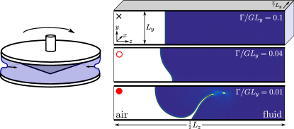
Figure 1: Left: Schematic of a cone and plate device. Right: Snapshots from full nonlinear simulations of the Giesekus model between hard walls. $\dot{\gamma}\tau=1.0$, $\theta=90^{\circ}$, $\alpha=0.4$, $\eta_{\rm a}/G\tau=0.01$.

In the $y$ direction we consider two different kinds of boundary condition. The first models the experimentally realisable case of shear between hard walls at $y=\pm L_{y}/2$, with no slip or permeation. The second gives the simplified biperiodic Lees-Edwards geometry, in which all quantities repeat periodically across shear-mapped points on the boundaries of box copies stacked in $y$, but with adjacent copies moving relative to each other at velocity $\dot{\gamma}L_{y}\hat{\mathbf{x}}$. Our numerically obtained threshold for the onset of edge fracture will prove in excellent agreement between these two. The simplified geometry allows analytical progress that is otherwise prohibitive.

The total stress $\mathbf{{T}}$ in any fluid element comprises an isotropic contribution $-p\mathbf{{I}}$ with pressure $p$, a Newtonian solvent contribution of viscosity $\eta_{\rm s}$, and a viscoelastic contribution $\mathbf{{\Sigma}}$ from the complex fluid (polymer chains, emulsion droplets, etc.), with a scale set by a constant modulus $G$. We assume creeping flow conditions, giving the force balance condition $\nabla.\mathbf{{T}}=0$, and therefore $\eta_{\rm s}\nabla^{2}\mathbf{{v}}+\nabla.\mathbf{{\Sigma}}-\nabla p=0$ inside the fluid and $\eta_{\rm a}\nabla^{2}\mathbf{{v}}-\nabla p=0$ in the air, with air viscosity $\eta_{\rm a}$. The pressure field $p(\mathbf{{r}},t)$ is determined by enforcing incompressibility, with the flow velocity $\mathbf{{v}}(\mathbf{{r}},t)$ obeying $\nabla.\mathbf{{v}}=0$. The dynamics of $\mathbf{{\Sigma}}$ is determined by a viscoelastic constitutive equation of the form

$$\partial_{t}\mathbf{{\Sigma}}+\mathbf{{v}}.\nabla\mathbf{{\Sigma}}=2G\mathbf{{D}}+\mathbf{{f}}(\mathbf{{\Sigma}},\nabla\mathbf{{v}})-\frac{1}{\tau}\mathbf{{g}}(\mathbf{{\Sigma}}),$$ (1)

where $\mathbf{{D}}=\tfrac{1}{2}(\nabla\mathbf{{v}}+\nabla\mathbf{{v}}^{T})$. The first two terms on the RHS capture the loading of viscoelastic stress in flow; the third relaxation back towards an unstressed state. The forms of $\mathbf{{f}}$ and $\mathbf{{g}}$ prescribe the precise model, and we shall simulate in what follows the Johnson-Segalman Johnson and Segalman (1977) and Giesekus Giesekus (1982) models, set out in SI . In the former, $\mathbf{{f}}$ contains a slip parameter $a$. In the latter, $\mathbf{{g}}$ contains an anisotropy parameter $\alpha$. Importantly, however, our predictions for edge fracture will depend on $a$ or $\alpha$ only via their appearance in the shear stress $\sigma\equiv T_{xy}$ and second normal stress difference $N_{2}\equiv T_{yy}-T_{zz}$. In this way, the key physics proves robust to choice of constitutive model. Indeed, most complex fluids show the low-shear scalings $\sigma\sim\dot{\gamma},N_{2}\sim-\dot{\gamma}^{2}$ of this model. An exception are non-Brownian suspensions Denn (2014), deferred to future work.

Our simulations model the air-fluid coexistence by a Cahn-Hilliard equation SI ; Anderson et al. (1998); Kusumaatmaja et al. (2016), with a mobility $M$ for air-fluid intermolecular diffusion, a scale $G_{\mu}$ for the free energy density of demixing, and a slightly diffuse air-fluid interface of thickness $l$, with surface tension $\Gamma=2\sqrt{2}G_{\mu}l/3$. Our linear stability analysis assumes a sharp interface, with a surface tension $\Gamma$. Our results for these two approaches agree fully.

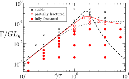
Figure 2: Edge fracture phase diagram for the Johnson-Segalman model in Lees-Edwards biperiodic shear. Solid line: phase boundary between stable and partially fractured states. Dashed line: prediction of Eqn. 8, with no adjustable parameters. Dotted line: Tanner’s prediction, with the prefactor adjusted to best-fit the simulations in the limit $\dot{\gamma}\tau\to 0$. $a=0.3$, $\eta_{\rm a}/G\tau=0.01$.

In unsheared equilibrium, the contact angle where the air-fluid interface meets the flow cell walls is denoted $\theta$. A value $\theta=90^{\circ}$ gives a vertical equilibrium interface; $\theta>90^{\circ}$ an interface convex into the air; and $\theta<90^{\circ}$ concave. In having a diffuse interface Kusumaatmaja et al. (2016), our simulations capture any motion of the contact line along the wall in flow. In the simplified biperiodic geometry the equilibrium interface is always vertical, mimicking $\theta=90^{\circ}$ with walls. As the initial condition for our shear simulations, we take a coexistence state first equilibrated without shear, with a small perturbation then added to the interface’s position $h(y)$ along the $z$ axis, $h\to h+10^{-8}\cos(n\pi y/L_{y})$, to trigger edge fracture, taking $n=1$ with walls and $n=2$ in the biperiodic geometry.

Important dimensionless quantities that we shall explore are the scaled surface tension $\Gamma/GL_{y}$, the Weissenberg number $\dot{\gamma}\tau$, the equilibrium contact angle $\theta$, and the air viscosity $\eta_{\rm a}/G\tau$. Less important parameters, which do not affect the physics once converged to their physically appropriate large or small limit are: the cell aspect ratio, $L_{z}/L_{y}=10.0$; the air gap size $(L_{z}-\Lambda)/L_{y}=3.0$; the small solvent viscosity SI ; the air-fluid interface width $l/L_{y}=0.01$, and the inverse mobility for intermolecular diffusion, $l^{2}/MG_{\mu}\tau=0.01-0.1$.

We now present our results. The basic phenomenon is exemplified by the three late-time snapshots of our nonlinear simulations of the Giesekus model between hard walls in Fig. 1, right. At any given imposed strain rate, an air-fluid interface with high surface tension is undisturbed by the flow and retains its equilibrium shape (top snapshot). We shall denote such states by a black cross in Fig. 2. For an intermediate surface tension the interface partially fractures, displacing in the $z$ direction a distance $O(L_{y})$ set by the gap between the rheometer plates in the $y$ direction, before settling to a new steady state shape, different from its unsheared equilibrium one. We denote these states by red open circles. Finally for a low surface tension, the interface fully fractures, displacing in the $z$ direction a distance $O(\Lambda)$ set by the sample width in that direction (red closed circles). Here the system never attains a new steady state: depending on the wetting angle and flow rate, the fluid may, eg, de-wet the wall, and/or air bubbles invade the fluid.

In Fig. 2, we collect into a phase diagram the results of simulations at many values of surface tension and shear rate, for the Johnson-Segalman model in the biperiodic geometry. (In the SI SI , we show that the phase boundary is essentially independent of model, geometry and equilibrium wetting angle $\theta$.) The red solid line marks the phase boundary between undisturbed and partially fractured interfacial states.

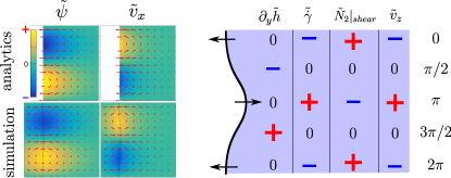
Figure 3: Left: eigenfunctions from analytic calculation (top) and simulation (bottom). (Analytics ignore the air phase, as shown by the white regions.) $\dot{\gamma}\tau=0.125$, $a=0.3$, $\Gamma/GL_{y}=0.0$, $\eta_{\rm a}/G\tau=0.01$, $q=2\pi/L_{y}$. Right: instability mechanism, discussed in text, with $0$ and $\pm$ symbols corresponding to the phase locations shown.

Within the biperiodic geometry, we now perform a linear stability analysis to derive an expression for this onset threshold, in the limit of low strain rates. To do so, we represent the state of the system as an underlying homogeneous time-independent base state (denoted by subscript $0$), corresponding to the initially unfractured case in which the interface is flat and the flow uniform. (Recall that our nonlinear simulations showed the phase boundary to be independent of the initial interfacial shape SI .) To this, we add a small perturbation (denoted by over-tildes) representing the precursor of edge fracture. For any given interfacial tension $\Gamma$ and imposed flow rate $\dot{\gamma}$, we then determine whether the perturbation grows towards an edge fractured state, or decays to leave a flat interface.

Accordingly, in the fluid bulk we write the velocity field $\mathbf{{v}}=\mathbf{{v}}_{0}+\tilde{\mathbf{{v}}}=(\dot{\gamma}y,0,0)+(\tilde{v}_{x},\partial_{z}\tilde{\psi},-\partial_{y}\tilde{\psi})$ and stress field $\mathbf{{T}}=\mathbf{{T}}_{0}+\tilde{\mathbf{{T}}}$. Our use of a streamfunction $\tilde{\psi}$ automatically ensures incompressibility. The force balance condition $\nabla.\mathbf{{T}}=0$ then simply becomes $\nabla.\tilde{\mathbf{{T}}}=0$. In the fluid bulk the $x$ component of force balance, and the curl of its $y,z$ components are respectively:

$$0 = \partial_{y}\tilde{T}_{xy}+\partial_{z}\tilde{T}_{xz},$$ (2a)

$$0 = \partial_{y}\partial_{z}(\tilde{T}_{yy}-\tilde{T}_{zz})+(\partial_{z}^{2}-\partial_{y}^{2})\tilde{T}_{yz}.$$ (2b)

We likewise write the $z$-position of the interface at any gap coordinate $y$ as $h_{0}+\tilde{h}(y)$. We further choose the origin of $z$ to lie at the interface, so $h_{0}=0$, with fluid for $z>0$ and air for $z<0$. The condition of force balance $\mathbf{{n}}.\mathbf{{T}}+\Gamma\mathbf{{n}}\nabla_{\rm int}.\mathbf{{n}}=0$ across this perturbed interface with normal $\mathbf{{n}}=\hat{\mathbf{z}}-\partial_{y}\tilde{h}\hat{\mathbf{y}}$ and $\nabla_{\rm int}$ the interfacial gradient operator gives componentwise linearised equations:

$$0 = \tilde{T}_{xz}|_{z=0^{+}}-\Delta\sigma\,\,\partial_{y}h,$$ (3a)

$$0 = \tilde{T}_{yz}|_{z=0^{+}}-N_{2}\,\partial_{y}h,$$ (3b)

$$0 = \tilde{T}_{zz}|_{z=0^{+}}+\Gamma\,\partial_{y}^{2}h,$$ (3c)

with $\Delta\sigma$ and $N_{2}$ the jumps in the shear and second normal stress difference across the interface, from fluid to air. ($N_{2}$ is always zero in the air, so we omit its $\Delta$ prefix.) Note we have assumed (for now) negligible stresses on the air side of the interface, $z=0^{-}$. The interface moves with the $z$-component of the fluid velocity:

$$\partial_{t}\tilde{h}=-\partial_{y}\tilde{\psi}|_{z=0}.$$ (4)

Finally, we must specify the perturbed stress components $\tilde{T}_{ij}$ in Eqns. 2 and 3. Each comprises a solvent contribution of viscosity $\eta_{\rm s}$, and a viscoelastic stress that follows Eqn. 1. For values of $(\Gamma/GL_{y},\dot{\gamma}\tau)$ only just across the instability threshold in Fig. 2, the interface will destabilise only very slowly and the viscoelastic stress will, for any instantaneous interfacial shape, be determined as the quasistatic solution of Eqn. 1. In the limit of small imposed shear rate $\dot{\gamma}$, this gives

$$\tilde{T}_{xy} = (G\tau+\eta_{\rm s})\partial_{y}\tilde{v}_{x}+O(\dot{\gamma}),$$ (5a)

$$\tilde{T}_{xz} = (G\tau+\eta_{\rm s})\partial_{z}\tilde{v}_{x}+O(\dot{\gamma}),$$ (5b)

$$\tilde{T}_{yy}-\tilde{T}_{zz} = 4(G\tau+\eta_{\rm s})\partial_{y}\partial_{z}\tilde{\psi}-2\dot{\gamma}G\tau^{2}b\partial_{y}\tilde{v}_{x},$$ (5c)

with $b=1-a$ and $\alpha$ in the Johnson-Segalman and Giesekus models respectively.

Substituting Eqn. 5 (with a counterpart expression for $\tilde{T}_{yz}$) into Eqns. 2, 3 gives finally a set of coupled partial differential equations for the perturbation to the bulk flow field, $\tilde{v}_{x}(y,z,t),\tilde{\psi}(y,z,t)$, and to the interface position $\tilde{h}(y,t)$. Solving these gives, to leading order in $\dot{\gamma}$ and at any wavevector $q$ in the $y$ direction,

$$\tilde{\psi}(y,z,t) = \left[Ae^{-qz}+Be^{-kz}\right]e^{iqy}e^{\omega t},$$

$$\tilde{v}_{x}(y,z,t) = Ce^{-qz}e^{iqy}e^{\omega t},$$

$$\tilde{h}(y,t) = iqDe^{iqy}e^{\omega t},$$ (6)

(ignoring a small term in $e^{-kz}$ in $\tilde{v}_{x}$), in which $k=q/\sqrt{1+\beta}$ with $\beta\approx b(1-b)\dot{\gamma}^{2}\tau^{2}$, and with known expressions for $A,B,C,D$ that we do not write. These eigenfunctions $\tilde{\psi}(y,z)$, $\tilde{v}_{x}(y,z)$ are shown in the left panel of Fig. 3 and agree fully with their counterparts from (the linear regime of) our fully nonlinear simulations in the same panel.

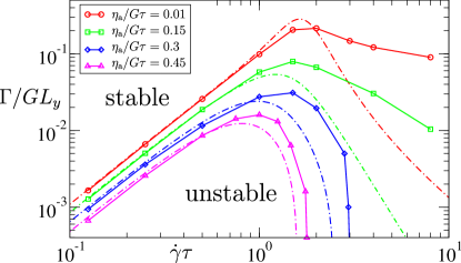
Figure 4: Threshold for onset of edge fracture instability in the Johnson-Segalman model in biperiodic shear, for various values of the viscosity $\eta_{\rm a}$ of the bathing medium. Solid lines: full nonlinear simulation. Dotted lines: linear stability analysis, valid in the limit $\dot{\gamma}\tau\to 0$. $a=0.3$, $\eta_{\rm s}/G\tau=0.15$.

Eqn. 6 tells us that perturbations at any wavevector $q$ will grow if their eigenvalue $\omega(q)>0$. We find

$$\omega=\frac{1}{2(G\tau+\eta_{\rm s})}\left[\frac{1}{2}\Delta\sigma\frac{d|N_{2}|}{d\dot{\gamma}}\middle/\frac{d\sigma}{d\dot{\gamma}}-\Gamma q\right].$$ (7)

The condition $\omega>0$ is most readily satisfied for the mode with the lowest wavevector that is consistent with the boundary conditions, $q=2\pi/L_{y}$. Accordingly, our final condition for an initially flat fluid-air interface to undergo edge fracture is given by

$$\frac{1}{2}\Delta\sigma\frac{d|N_{2}(\dot{\gamma})|}{d\dot{\gamma}}\bigg{/}\frac{d\sigma}{d\dot{\gamma}}>\frac{2\pi\Gamma}{L_{y}}.$$ (8)

This criterion is marked by the dashed line in Fig. 2, and fully agrees at low shear rates with the onset of fracture in our numerical simulations.

We now compare Eqn. 8 with Tanner’s prediction of $|N_{2}|>2\Gamma/3R$, with $R$ the radius of an assumed initially semicircular interfacial crack. Clearly, $R$ must now be replaced by the dominant wavelength $L_{y}$. Disregarding $O(1)$ prefactors, the important difference between Tanner’s prediction and ours then lies in replacing

$$|N_{2}|\to\frac{1}{2}\;\Delta\sigma\frac{d|N_{2}|}{d\dot{\gamma}}\bigg{/}\frac{d\sigma}{d\dot{\gamma}}.\;\;$$ (9)

Given negligible air viscosity, the jump $\Delta\sigma$ in shear stress across the interface between the fluid and air simply equals the shear stress $\sigma$ in the fluid. For most complex fluids (excluding non-Brownian suspensions), in the limit of small shear rates, $N_{2}\sim-\dot{\gamma}^{2}$ and $\sigma\sim\dot{\gamma}$. Tanner’s $|N_{2}|$ on the LHS of (9) then simply equals our expression on the RHS. In contrast, at higher shear rates these simple power laws no longer (in general) hold, and our prediction departs from Tanner’s, as seen in Fig. 2. Indeed, Tanner predicts the critical surface tension to increase monotonically with shear rate. The non-monotonicity that we find follows because $\sigma$ and $|N_{2}|$ both initially increase with $\dot{\gamma}$, before $N_{2}(\dot{\gamma})$ saturates to a constant at high shear rates, such that $dN_{2}/d\dot{\gamma}\to 0$.

Our results also explain the mechanism of instability as follows. Were the interface to remain perfectly flat, the jump $\Delta\sigma$ in shear stress across it would be consistent with force balance. However, any small interfacial tilt $\partial_{y}\tilde{h}$ (first column of Fig. 3, right) exposes this jump. To maintain force balance across the interface, a counterbalancing perturbation $\tilde{T}_{xz}=iqh\Delta\sigma$ is then required (Eqn. 3a). To maintain the $x$-component of force balance in the fluid bulk (Eqn. 2a), a corresponding perturbation $\tilde{T}_{xy}$ is then needed, achieved via a perturbation $\tilde{\dot{\gamma}}=\partial_{y}\tilde{v}_{x}=qh\Delta\sigma/\sigma^{\prime}(\dot{\gamma})$ in the shear rate (second column of Fig. 3, right). The second normal stress $N_{2}\approx-bG\tau^{2}\dot{\gamma}^{2}$ in the fluid bulk then suffers a corresponding perturbation (second term in Eqn. 5c) $\tilde{T}_{yy}-\tilde{T}_{zz}|_{\rm shear}=-qh\Delta\sigma\,|N_{2}|^{\prime}(\dot{\gamma})/\sigma^{\prime}(\dot{\gamma})$ (third column of Fig. 3, right). This must be counterbalanced (at zero surface tension at least) by an equal and opposite extensional perturbation (first term in Eqn. 5c): $\tilde{T}_{yy}-\tilde{T}_{zz}|_{\rm ext}=4G\tau\partial_{y}\partial_{z}\tilde{\psi}=-4G\tau\partial_{z}\tilde{v}_{z}=4G\tau q\tilde{v}_{z}$. This requires a $z$-component of fluid velocity (fourth column of Fig. 3, right), which convects the interface, $\partial\tilde{h}/\partial t=\tilde{v}_{z}=\tfrac{1}{4}\Delta\sigma h\,|N_{2}|^{\prime}(\dot{\gamma})/G\tau\sigma^{\prime}(\dot{\gamma})$, enhancing its original tilt with a growth rate $\omega=\tfrac{1}{4}\Delta\sigma\,|N_{2}|^{\prime}(\dot{\gamma})/G\tau\sigma^{\prime}(\dot{\gamma})$, consistent with Eqn. 7 at zero surface tension, noting that $\eta_{\rm s}$ is small. This mechanism resembles in spirit that of instabilities between layered viscoelastic fluids Hinch et al. (1992); Wilson and Rallison (1997); Fielding (2010).

Finally, our results suggest a recipe via which edge fracture might be mitigated. By immersing the flow cell in an immiscible Newtonian ‘bathing fluid’ with a viscosity larger than that of air, more closely matched to that of the study-fluid, the jump $\Delta\sigma$ in shear stress between the study and bathing fluids, which is a key factor in driving the instability, will be reduced. This is explored in Fig. 4. The red solid line shows the onset threshold for a bathing fluid of negligible viscosity, such as air; and the green, blue and magenta lines for successively increasing values of the bathing fluid’s viscosity, each giving increased stability. The dashed lines show linear stability results recalculated with non-zero bath viscosity, in excellent agreement. Clearly, choosing a bathing fluid with as a high a possible surface tension with the test fluid will also help stability.

To summarise, we have derived an exact expression for the onset of edge fracture in complex fluids, shown it to agree with numerical simulations, and provided the first mechanistic understanding of edge fracture. We have also suggested a way of mitigating the phenomenon experimentally. Given the status of edge fracture as a crucially limiting factor in experimental rheology, this suggests a route to accessing stronger flows than hitherto.

Acknowledgements – The research leading to these results has received funding from the European Research Council under the EU’s 7th Framework Programme (FP7/2007-2013) / ERC grant number 279365. The authors thank Peter Olmsted for discussions and Mike Cates and Roger Tanner for a critical reading of the manuscript.

Supplementary Material for:
“Edge fracture in complex fluids”

This supplementary information is divided into four parts. In the first, we define the details of the constitutive models for which results are presented in the main text. In the second, we show those results to be independent of this choice of constitutive model. In the third, we show robustness to the boundary conditions at edges of the flow cell. Finally, we outline our numerical scheme.

I Definition of constitutive models

As discussed in the main text, the dynamics in flow of the viscoelastic stress $\mathbf{{\Sigma}}$ is determined by a constitutive equation of the general form

$$\partial_{t}\mathbf{{\Sigma}}+\mathbf{{v}}.\nabla\mathbf{{\Sigma}}=2G\mathbf{{D}}+\mathbf{{f}}(\mathbf{{\Sigma}},\nabla\mathbf{{v}})-\frac{1}{\tau}\mathbf{{g}}(\mathbf{{\Sigma}}),$$ (S1)

where $G$ is the viscoelastic modulus and $\tau$ is the relaxation timescale. The forms of $\mathbf{{f}}$ and $\mathbf{{g}}$ depend on the constitutive model in question, and we now specify these for the two models explored in the main text.

The Johnson-Segalman model Johnson1977a has

$$\mathbf{f}\left(\mathbf{\Sigma},\mathbf{\nabla v}\right) =\left(\mathbf{\mathbf{\Sigma}\mathbf{\Omega}-\Omega}\mathbf{\Sigma}\right)+a\left(\mathbf{D}\mathbf{\Sigma}+\mathbf{\Sigma}\mathbf{D}\right),$$ (S2)

$$\mathbf{g}\left(\mathbf{\Sigma}\right) =\mathbf{\Sigma},$$ (S3)

in which $\mathbf{{D}}=\tfrac{1}{2}(\nabla\mathbf{{v}}+\nabla\mathbf{{v}}^{T})$ and $\mathbf{{\Omega}}=\tfrac{1}{2}(\nabla\mathbf{{v}}-\nabla\mathbf{{v}}^{T})$ with $\nabla\mathbf{{v}}_{\alpha\beta}=\partial_{\alpha}v_{\beta}$. The parameter $a$ describes the slip of the viscoelastic component (eg, polymer chains) relative to affine flow. It has values in the range $-1\leq a\leq 1$. Define the adimensional viscoelastic shear stress, second normal stress difference and shear rate as

$$\hat{\sigma}_{\rm p}=\Sigma_{xy}/G,\quad\hat{N}_{2}=\left(\Sigma_{yy}-\Sigma_{zz}\right)/G,\quad\hat{\dot{\gamma}}=\dot{\gamma}\tau$$ (S4)

respectively. Then in steady homogeneous simple shear flow, as function of the imposed shear rate $\dot{\gamma}$, these are given as Skorski2011

$$\hat{\sigma}_{\rm p}=\frac{\hat{\dot{\gamma}}}{1+(1-a^{2})\hat{\dot{\gamma}}^{2}},$$ (S5)

$$\hat{N}_{2}=\frac{\left(-1+a\right)\hat{\dot{\gamma}}^{2}}{1+(1-a^{2})\hat{\dot{\gamma}}^{2}}.$$ (S6)

The Giesekus model Giesekus1982a has

$$\mathbf{f}\left(\mathbf{\Sigma},\mathbf{\nabla v}\right) =\left(\mathbf{\mathbf{\Sigma}\mathbf{\Omega}-\Omega}\mathbf{\Sigma}\right)+\left(\mathbf{D}\mathbf{\Sigma}+\mathbf{\Sigma}\mathbf{D}\right),$$ (S7)

$$\mathbf{g}\left(\mathbf{\Sigma}\right) =\mathbf{\Sigma}+\frac{\alpha}{G}\mathbf{\Sigma}^{2}.$$ (S8)

Here $\alpha$ is an anisotropy parameter, which models an enhanced rate of stress relaxation in regimes where the polymer chains are more strongly aligned. In steady homogeneous simple shear flow, the adimensional viscoelastic shear stress and second normal stress difference are given as Giesekus1982a

$$\hat{\sigma}_{\rm p} = \frac{(1+\hat{N}_{2})^{2}\hat{\dot{\gamma}}}{1-(1-2\alpha)\hat{N}_{2}},$$

$$\hat{N}_{2} = \frac{\left(\Lambda-1\right)}{1+(1-2\alpha)\Lambda},$$ (S9)

in which

$$\Lambda^{2}=\frac{1}{8\alpha(1-\alpha)\hat{\dot{\gamma}}^{2}}\left[\sqrt{1+16\alpha(1-\alpha)\hat{\dot{\gamma}}^{2}}-1\right].$$ (S10)

In both models, the total steady state shear stress $\sigma(\dot{\gamma})=G\hat{\sigma}_{\rm p}(\dot{\gamma})+\eta_{\rm s}\dot{\gamma}$ comprises the sum of the viscoelastic part just defined and a Newtonian contribution of viscosity $\eta_{\rm s}$. For parameter values $|a|<1$ and $\eta_{\rm s}/G\tau<1/8$ in the Johnson-Segalman model, the total shear stress $\sigma(\dot{\gamma})$ is a non-monotonic function of the imposed shear rate, allowing the coexistence of bands of differing shear rates at a common value of the total shear stress: a phenomenon known as shear banding. We consider here only non-shear-banded flows, taking $a=0.3$ and $\eta_{\rm s}/G\tau=0.15$ in our numerical simulations. In the Giesekus model, $\sigma(\dot{\gamma})$ is a monotonic function for $\alpha\leq 1/2$ for any $\eta_{\rm s}$ Giesekus1982a . We set $\alpha=0.4$ and $\eta_{\rm s}/G\tau=0.01$ in our numerics, again avoiding shear-banding. In both models (provided $a<1$ or $\alpha>0$), the second normal stress is negative, scaling as $-\dot{\gamma}^{2}$ at low shear rates and saturating to a negative constant at high shear rates.

II Robustness to constitutive model

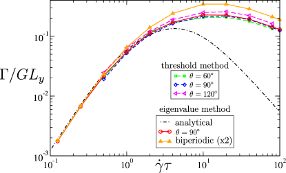
Figure S1: Threshold for the onset of edge fracture instability in the Giesekus model sheared between hard walls (open symbols) and in the biperiodic geometry (closed symbols). Black dash-dotted line shows our analytical prediction of Eqn. 8 in the main text. Parameters: $\alpha=0.4$, $\eta_{\rm s}/G\tau=0.01$, $\eta_{\rm a}/G\tau=0.01$.

We now demonstrate the robustness of our results with respect to this choice of constitutive model. Recall that Fig. 2 of the main text showed the threshold for the onset of edge fracture obtained from our numerical simulations of the Johnson-Segalman model in the biperiodic geometry, and the agreement with it at low strain rates of our analytical prediction of Eqn. 8 of the main text. We now explore this same comparison for the Giesekus model. See Fig. S1, in which the solid triangles show the threshold obtained from our numerical simulations in the biperiodic geometry, and the long-dashed line shows the prediction of Eqn. 8 of the main text. Excellent agreement is again obtained at low shear rates. Both constitutive models therefore give behaviour in accordance with our central prediction of Eqn. 8 in the main text.

Comparing Fig. S1 with Fig. 2 of the main text also shows that both models capture a re-entrant region of stability against edge fracture at large shear-rates. As discussed in the main text, this arises from the saturation of $N_{2}$ at high shear rates. The smaller solvent viscosity in the Giesekus simulations however postpones this to higher strain rates than in the Johnson-Segalman simulations.

III Robustness to boundary condition

Recall that in the main text we considered two different boundary conditions: the first corresponding to the experimentally realisable geometry in which the boundaries of the flow cell in the flow-gradient direction comprise hard walls, and the second to theoretically simplified Lees-Edwards sheared periodic boundary conditions.

To check for robustness with respect to this choice of boundary condition, in Fig. S1 we compare the threshold for the onset of edge fracture obtained from simulations of a cell with hard walls in the flow-gradient direction, for three different values of the equilibrium contact angle, $\theta=60,90,120^{\circ}$, with that obtained in simulations adopting Lees-Edwards biperiodic shear. Good qualitative agreement is seen across these four cases at all shear rates, with excellent quantitative agreement at low shear rates. (Note that the lowest possible wavevector in the biperiodic geometry is twice that in the walled geometry. For consistency we accordingly rescaled the critical surface tension by a factor two in that case.)

To identify this threshold, we first defined the steady-state displacement of the interface to be $d=\max(h(y))-\min(h(y))$, with $d_{0}$ the value of this quantity in an unsheared system. We then define the onset threshold at any imposed shear rate to be the value of the surface tension $\Gamma$ at which $d(\Gamma)$ (in shear) obeys $d(\Gamma)-d_{0}=0.1$. For a contact angle $\theta=90^{\circ}$ in the simulations with walls, and in all the simulations in biperiodic shear, the interface between the fluid and air is initially flat and we can alternatively identify onset of edge fracture by the surface tension at which the eigenvalue calculated in the main text first becomes positive. As seen in Fig. S1, these two methods of identifying onset agree well.

IV Numerical scheme

In our analytical calculations we assume an infinitely sharp interface of surface tension $\Gamma$ between the sheared slab of viscoelastic fluid and the outside air. In our simulations we instead explicitly model this coexistence of fluid and air using a phase field approach with an order parameter $\phi$, which obeys Cahn-Hilliard dynamics Bray1994

$$\partial_{t}\phi+\mathbf{{v}}.\nabla\phi =M\nabla^{2}\mu.$$ (S11)

Here $M$ is the molecular mobility, which we assume constant. The chemical potential

$$\mu =G_{\mu}\left(-\phi+\phi^{3}-\ell^{2}\nabla^{2}\phi\right),$$ (S12)

in which $G_{\mu}$ sets the overall scale for the free energy of demixing per unit volume. This captures the coexistence of a fluid phase in which $\phi=1$ with an air phase in which $\phi=-1$, with the two phases separated by a slightly diffuse interface of thickness $\ell$ and surface tension

$$\Gamma=\frac{2\sqrt{2}}{3}G_{\mu}\ell.$$ (S13)

This contributes an additional source term of the form $-\phi\nabla\mu$ to the Stokesian force balance condition, as discussed in the main text. The modulus $G$ and relaxation time $\tau$ that appear in the viscoelastic constitutive equation are then made functions of $\phi$, such that viscoelastic stresses only arise in the fluid phase.

Where the fluid meets the hard walls of a flow cell, the boundary conditions are taken to be Yue2010 ; Dong2012

$$\mathbf{n}\cdot\nabla\mu =0,$$ (S14)

$$\mathbf{n}\cdot\nabla\phi =\frac{-1}{\sqrt{2}\ell}\cos{\theta}\left(1-\phi^{2}\right).$$ (S15)

with $\mathbf{n}$ the outward unit vector normal to the wall. The parameter $\theta$ defines the equilibrium contact angle the interface between the air and fluid makes with the wall.

At each numerical timestep we first solve the Stokes balance condition to update the fluid velocity field $\mathbf{v}$ at fixed phase field $\phi$ and polymer stress $\mathbf{\Sigma}$, using a streamfunction formulation to ensure incompressible flow. We then in turn update the phase field and viscoelastic stress, with the velocity field fixed. The advective terms are implemented using a third order upwinding scheme pozrikidis2011introduction , and any spatially local terms (which in fact only arise in the viscoelastic constitutive equation) using an explicit Euler scheme numericalrecipes . To implement the spatially diffusive terms, in the Lees Edward biperiodic geometry we use a Fourier spectral method. With walls present, we instead use a hybrid method: again with Fourier modes in the periodic vorticity direction $z$, and with finite differencing numericalrecipes in the flow gradient direction $y$. All numerical results presented are converged on decreasing mesh size and increasing mode number.

References

- Lee et al. (1992) C. S. Lee, B. C. Tripp, and J. J. Magda, Rheol. Acta 31, 306 (1992).
- Inn et al. (2005) Y. W. Inn, K. F. Wissbrun, and M. M. Denn, Macromolecules 38, 9385 (2005).
- Sui and McKenna (2007) C. Sui and G. B. McKenna, Rheol. Acta 46, 877 (2007).
- Schweizer and Stöckli (2008) T. Schweizer and M. Stöckli, J. Rheol. 52, 713 (2008).
- Mattes et al. (2008) K. M. Mattes, R. Vogt, and C. Friedrich, Rheol. Acta 47, 929 (2008).
- Jensen and Christiansen (2008) E. A. Jensen and J. d. C. Christiansen, J. Non-Newtonian Fluid Mech. 148, 41 (2008).
- Dai et al. (2013) S.-C. Dai, E. Bertevas, F. Qi, and R. I. Tanner, J. Rheol. 57, 493 (2013).
- Eggers and Villermaux (2008) J. Eggers and E. Villermaux, Rep. Prog. Phys. 71, 036601 (2008).
- (9) G. H. McKinley, Visco-Elasto-Capillary Thinning and Break-Up of Complex Fluids, in Annual Rheology Reviews, edited by D. M. Binding and K. Walters (British Society for Rheology, Aberystwyth, 2005), pp. 1—48.
- Tanner and Keentok (1983) R. I. Tanner and M. Keentok, J. Rheol. 27, 47 (1983).
- Keentok and Xue (1999) M. Keentok and S.-C. Xue, Rheol. Acta 38, 321 (1999).
- Note (1) We consider throughout positive flow rates, . For negative flow rates we must replace by . For most fluids .
- Onuki (1997) A. Onuki, J. Phys. Soc. Jpn. 66, 1836 (1997).
- Johnson and Segalman (1977) M. Johnson and D. Segalman, J. Non-Newtonian Fluid Mech. 2, 255 (1977).
- Giesekus (1982) H. Giesekus, J. Non-Newtonian Fluid Mech. 11, 69 (1982).
- (16) See Supplementary Material (below)..
- Denn (2014) M. M. Denn and J. F. Morris, Annu. Rev. Chem. Biomol. Eng. 5, 203 (2014).
- Anderson et al. (1998) D. M. Anderson, G. B. McFadden, and A. A. Wheeler, Annu. Rev. Fluid Mech. 30, 139 (1998).
- Kusumaatmaja et al. (2016) H. Kusumaatmaja, E. J. Hemingway, and S. M. Fielding, J. Fluid Mech. 788, 209 (2016).
- Hinch et al. (1992) E. Hinch, O. Harris, and J. M. Rallison, J. Non-Newtonian Fluid Mech. 43, 311 (1992).
- Wilson and Rallison (1997) H. J. Wilson and J. M. Rallison, J. Non-Newtonian Fluid Mech. 72, 237 (1997).
- Fielding (2010) S. M. Fielding, Phys. Rev. Lett. 104, 198303 (2010).

References

- (1) M. Johnson and D. Segalman. A model for viscoelastic fluid behavior which allows non-affine deformation. J. Non-Newtonian Fluid Mech., 2, 255–270, 1977.
- (2) S. Skorski and P. D. Olmsted. Loss of solutions in shear banding fluids driven by second normal stress differences. J. Rheol., 55, 1219, 2011.
- (3) H. Giesekus. A simple constitutive equation for polymer fluids based on the concept of deformation-dependent tensorial mobility. J. Non-Newtonian Fluid Mech., 11, 69–109, 1982.
- (4) A. Bray. Theory of phase-ordering kinetics. Adv. Phys., 43, 357–459, 1994.
- (5) P. Yue, C. Zhou, and J. J. Feng. Sharp-interface limit of the Cahn-Hilliard model for moving contact lines. J. Fluid Mech., 645, 279, 2010.
- (6) S. Dong. On imposing dynamic contact-angle boundary conditions for wall-bounded liquid–gas flows. Comput. Methods Appl. Mech. Eng., 247-248, 179–200, 2012.
- (7) C. Pozrikidis. Introduction to Theoretical and Computational Fluid Dynamics. Oxford University Press, New York, 2011.
- (8) W. H. Press, S. A. Teukolsky, W. T. Vetterling, and B. P. Flannery. Numerical Recipes in C (2nd Ed.): The Art of Scientific Computing. Cambridge University Press, New York, NY, USA, 1992.