Decompositions of surface flows

Abstract.

Under a regularity condition for the singular point set, every flow on a compact surface can be constructed by glueing four kinds of invariant open subsets, which are flow boxes, transverse/periodic annuli, and locally dense Q-sets. In particular, Morse-Smale flows on compact surfaces can be constructed by glueing the boundaries of invariant flow boxes and invariant transverse annuli, and Hamiltonian flows on compact surfaces with finitely many singular points can be constructed by glueing the boundaries of invariant periodic annuli. Using the decompositions, we construct a finite complete invariant for surface flows of finite type. In fact, although degeneracy of singular points implies uncountably many local topological equivalence classes and the set of topological equivalence classes of minimal flows on a torus is uncountable, we enumerate the set of topological equivalence classes of flows with at most finitely many limit cycles but without non-closed recurrent orbits or degenerate singular points on compact surfaces using finite labelled graphs.

1. Introduction

1.1. On surface flows

Flows on surfaces are one of the most classical objects in dynamical systems and are wildly studied. For instance, the Poincaré-Bendixson theorem states the description of limit sets of points and is generalized in several ways [1, 4, 9, 11, 16, 17, 25, 29, 40, 44, 45]. In particular, the following statement holds (see for example [29]): The $\omega$-limit set of an orbit of a flow with finitely many fixed points on a compact surface is either a closed orbit, a semi-attracting limit circuit, or a Q-set. A part of this classification is based on the following Maǐer’s result [23] (see Theorem 2.4.4 p.32 [29], Theorem 4.2 [3] for general cases, and Theorem 19 [21] for orientable hyperbolic cases for details): Any point contained in an $\omega$-limit set of some point for a flow on a compact surface whose $\omega$-limit set contains non-closed orbits is positively recurrent.

On the other hand, stability and genericity of flows on surfaces are studied. In fact, structural stability are introduced by Andronov and Pontryagin [2]. Moreover, they showed the structural stability and open denseness of Morse-Smale flows on spheres. In addition, Peixoto [31] generalized the result as follows: A vector field $v\in\chi^{r}(S)$ is structurally stable if and only if $v\in\Sigma^{r}(S)$, where $\chi^{r}(S)$ ($r\in\mathbb{Z}_{\geq 1}$) is the set of $C^{r}$-vector fields (with the $C^{r}$- topology) on an orientable closed surface $S$ and $\Sigma^{r}(S)$ is the subset of $\chi^{r}(S)$ formed by the Morse-Smale $C^{r}$-vector fields on $S$. Moreover, $\Sigma^{r}(S)$ is open and dense in $\chi^{r}(S)$. When $M$ is a non-orientable closed surface, Pugh’s $C^{1}$-Closing Lemma implies [32, 33] that $\Sigma^{1}(M)$ is dense and that the Peixoto’s work holds for the case in which the non-orientable genus of $M$ is less than five [10, 19]. On $C^{r}$-Hamiltonian vector fields ($r\in\mathbb{Z}_{\geq 1}$), a Hamiltonian vector field $v\in\mathcal{H}^{r}(S)$ is structurally stable in $\mathcal{H}^{r}(S)$ if and only if $v\in\mathcal{H}^{r}_{*}(S)$, and that $\mathcal{H}^{r}_{*}(S)$ is open dense in $\mathcal{H}^{r}(S)$ [18], where $\mathcal{H}^{r}(S)$ is the set of Hamiltonian $C^{r}$ vector fields on an orientable closed connected surface $S$ and $\mathcal{H}^{r}_{*}(S)$ is the set of Hamiltonian $C^{r}$ vector fields whose singular points are non-degenerate and whose saddle connection are self-connected.

The smoothability of flows on surfaces are described by the following Gutierrez’s smoothing theorem [10]: Each flow on a compact surface is topologically equivalent to a $C^{1}$-flow. Moreover, if any minimal sets are closed orbits or invariant tori, then such flows are topologically equivalent to $C^{\infty}$-flows.

1.2. Topological invariants of flows on surfaces

There are several topological invariants of hyperbolic flows and their generalizations. For instance, a basic result of Morse theory says that gradient flows of Morse functions on closed surfaces are characterized by the set of saddles and their separatrices, which are finite directed graphs. The Morse theory for gradient vector fields on compact surfaces is extended to an index theory for Smale flows on compact surfaces using Lyapunov graphs [8], which are generalizations of the quotient spaces of gradient functions. Recall that a flow is Smale if (1) its chain recurrent set has a hyperbolic structure and its dimension is less than or equal to one; and (2) it satisfies the transverse condition. In [35], a characterization of Lyapunov graphs associated with smooth surface flows is presented. It is known that Peixoto graph is a complete invariant for Morse-Smale flows without limit cycles (i.e. Morse flows), three-colour graph is a complete invariant for Morse-Smale flows [30], and an equipped graph [14] is a complete invariant for $\Omega$-Stable flows on compact surfaces, which are “Morse-Smale flow without non-existence of heteroclinic separatrices”.

On the other hand, there are complete invariants for non-hyperbolic flows. In [28], non-wandering flows with finitely many singular points on compact surfaces are classified up to a graph-equivalence by using a topological invariant, called a Conley-Lyapunov-Peixoto graph, which is equipped with rotation and weight functions. In addition, the following assertion was stated in the papers [22, 26, 27]:

An orbit complex (also called separatrix configuration) of a flow is also a complete invariant for the set of flows with “finitely many separatrices” in the sense of Markus.

Though these papers are referred more than one hundred papers as mentioned in [5], Buendía and López have pointed out that the assertion does not hold. In fact, the orbit complex is not a complete invariant for flows having “finitely many separatrices” in the sense of Markus and it is not a complete invariant for flows with finitely many singular points but without limit separatrices in the sense of Markus [5]. One of their counterexamples is a toral flow which consists of one singular point and non-recurrent orbits. In particular, the proof of a Poincaré-Hopf theorem for continuous flows with “finitely many separatrices” does not work. In [5], the authors have modified the invariant into a complete invariant, called a separatrix configuration, for flows whose essential singular points are at most finite. By definition of separatrix configuration in the sense of Buendía and López (see Definition 2.2 [5] for details), note that the separatrix configuration contains the complement of the interior of the union of non-recurrent orbits, and so that it contains infinitely many data in general. Notice that their definition of $\alpha^{\prime}(p)$ (resp. $\omega^{\prime}(p)$) is slightly different from the original one (see [22, 26, 27]), but these definitions correspond to each other except non-closed recurrent orbits. Therefore definitions of orbit complexes of flows without non-closed recurrent orbits correspond to each other even if they use the different definitions of $\alpha^{\prime}(p)$ (resp. $\omega^{\prime}(p)$). On the other hand, we show that an orbit complex of flows of finite type which is equipped with additional orders is a complete invariant, and that the orbit complex is also a complete invariant under the assumption that the multi-saddle connection diagram is the saddle connection diagram containing no non-self-connected separatrices (i.e. each multi-saddle is either a saddle without heteroclinic multi-saddle separatrices or a $\partial$-saddle without separatrices connecting another multi-saddles outside of the same boundary) (see Theorem C).

We describe the properties of the border points of a flow $v$ on a compact surface with a regularity condition for the singular point set. Moreover, each connected component of the complement of the border point set is either an open disk, an open annulus, a torus, a Klein bottle, an open Möbius band, or an essential open subset consisting of locally dense orbits (see Theorem A). Similarly, we can also the flow $v$ glueing four kinds of invariant open subsets (flow boxes, transverse/periodic annuli, and locally dense Q-sets) (see Theorem B). Here a Q-set is the closure of a non-closed recurrent orbit. In addition, although the existence of degenerate singular points can imply uncountably many local topological equivalence classes and the set of topological equivalence classes of minimal flows (resp. Denjoy flows) on a torus is uncountable, a flow with at most finitely many limit cycles but without non-degenerate singular points or recurrent orbits on a compact surface can be reconstructed from the finite data (see Theorem 8.3). In other words, we construct a finite complete invariant for surface flows of finite type. Note that all Hamiltonian flows with finitely many singular points and all Morse-Smale flows are flows of finite type, and that each of three conditions (i.e. quasi-regularity of singular points, non-existence of recurrent orbits, finiteness of limit cycles) in the definition of “finite type” is necessary for finite representability.

1.3. Statements of main results

Roughly speaking, under a regularity condition on the singular point set, all the flows on compact surfaces can be constructed by glueing seven (resp. four) kinds of invariant open subsets (see Theorem A (resp. Theorem B) for details).

More precisely, we define blow-downs of a surface and their flows as follows (see Figure 1):

Figure 1. Canonical quotient mappings induced by the metric completion and the collapse.

Let $v$ be a flow on a surface $S$ whose singular point set has at most finitely many connected components. Since the singular point set $\mathop{\mathrm{Sing}}(v)$ is closed, the complement $S-\mathop{\mathrm{Sing}}(v)$ is open and so a surface. In particular, the set difference $S-(\mathop{\mathrm{Sing}}(v)\cup\partial S)$ is an open surface without boundary. Fix a Riemannian metric on $S$ such that $\mathop{\mathrm{Sing}}(v)$ is bounded. Denote by $S_{\mathrm{mc}}$ the metric completion of the complement $S-\mathop{\mathrm{Sing}}(v)$. Identifying the union $\partial$ of new boundary components with the new singular points, define a flow $v_{\mathrm{mc}}$ on $S_{\mathrm{mc}}$ such that $O_{v}(x)=O_{v_{\mathrm{mc}}}(x)$ for any point $x\in S-\mathop{\mathrm{Sing}}(v)=S_{\mathrm{mc}}-\mathop{\mathrm{Sing}}(v_{\mathrm{mc}})$ up to topological equivalence. Then $\partial=\mathop{\mathrm{Sing}}(v_{\mathrm{mc}})$ and so $S-\mathop{\mathrm{Sing}}(v)=S_{\mathrm{mc}}-\mathop{\mathrm{Sing}}(v_{\mathrm{mc}})$. By Theorem 3 [34], each connected component of the open surface $S-(\mathop{\mathrm{Sing}}(v)\cup\partial S)$ without boundary is homeomorphic to the resulting surface from a closed surface by removing a closed totally disconnected subset. Therefore, collapsing each connected component of $\mathop{\mathrm{Sing}}(v_{\mathrm{mc}})$ into a singular point, we obtain the resulting flow $v_{\mathrm{col}}$ with totally disconnected singular points, called the blow-down flow of $v$, on the resulting surface $S_{\mathrm{col}}$, called the blow-down surface, up to topological equivalence. Then $O_{v}(x)=O_{v_{\mathrm{mc}}}(x)=O_{v_{\mathrm{col}}}(x)$ for any point $x\in S-\mathop{\mathrm{Sing}}(v)=S_{\mathrm{mc}}-\mathop{\mathrm{Sing}}(v_{\mathrm{mc}})=S_{\mathrm{col}}-\mathop{\mathrm{Sing}}(v_{\mathrm{col}})$. Notice that $S_{\mathrm{mc}}$ and $S_{\mathrm{col}}$ may have infinitely many connected components but that each connected component of $S_{\mathrm{col}}$ is a compact surface.

Recall that a flow on a surface is quasi-regular if any singular points are either multi-saddles, sinks, $\partial$-sinks, sources, $\partial$-sources, or centers (see Figure 2).

Figure 2. Multi-saddles, a sink, a $\partial$-sink, a source, a $\partial$-source, and a center.

A flow on a surface with finitely many connected components of the singular point set is regular-like if the blow-down flow is quasi-regular. Then a connected component of the singular point set which corresponds to a multi-saddle is called the weak saddle. An orbit is from or to a weak saddle if it is from or to a multi-saddle with respect to the blow-down flow $v_{\mathrm{col}}$. For a flow $v$ on a compact surface, put

$$\mathop{\mathrm{Bd}_{0}}(v):=\mathop{\mathrm{Sing}}(v)\sqcup\partial^{-}\mathop{\mathrm{Per}}(v)\sqcup\mathop{\mathrm{P}_{\mathrm{semi}}}(v)\sqcup\mathrm{E}(v)$$

where $\mathop{\mathrm{Per}}(v)$ (resp. $\mathrm{E}(v)$) is the union of periodic (resp. nowhere dense recurrent) orbits and $\mathop{\mathrm{P}_{\mathrm{semi}}}(v)$ is the union of non-recurrent orbits from or to weak saddles. Here $\partial^{-}A:=A-\mathrm{int}A$ for any subset $A\subseteq S$. By definition, any regular-like flow $v$ on a compact surface $S$ and the blow-down flow $v_{\mathrm{col}}$ on the blow-down surface $S_{\mathrm{col}}$ correspond to each other on the complement $S-\mathop{\mathrm{Bd}}_{0}(v)=S_{\mathrm{col}}-\mathop{\mathrm{Bd}}_{0}(v_{\mathrm{col}})$ up to topological equivalence. For a point $z\in S_{\mathrm{col}}$, denote by $\alpha_{v_{\mathrm{col}}}(z)$ the $\alpha$-limit set of $z$ in $S_{\mathrm{col}}$ with respect to $v_{\mathrm{col}}$ and by $\omega_{v_{\mathrm{col}}}(z)$ the $\omega$-limit set of $z$ in $S_{\mathrm{col}}$ with respect to $v_{\mathrm{col}}$. We describe the decomposition of a regular-like flow on a compact surface.

Theorem A.

Each connected component of $S-\mathop{\mathrm{Bd}}_{0}(v)$ for a regular-like flow $v$ on a compact surface $S$ is one of the following seven invariant open subsets exclusively:
$(1)$ A flow box in $\mathrm{P}(v)$,
$(2)$ An annulus in $\mathrm{P}(v)$,
$(3)$ An annulus in $\mathop{\mathrm{Per}}(v)$,
$(4)$ A torus in $\mathop{\mathrm{Per}}(v)$,
$(5)$ A Klein bottle in $\mathop{\mathrm{Per}}(v)$,
$(6)$ A Möbius band in $\mathop{\mathrm{Per}}(v)$, or
$(7)$ An essential subset in $\mathrm{LD}(v)$.

Moreover, the following statements hold:
$(a)$ For any connected component $U$ in $\mathrm{P}(v)\setminus\mathop{\mathrm{Bd}}_{0}(v)$ and for any points $x,y\in U$, we have $\alpha_{v_{\mathrm{col}}}(x)=\alpha_{v_{\mathrm{col}}}(y)$ and $\omega_{v_{\mathrm{col}}}(x)=\omega_{v_{\mathrm{col}}}(y)$.
$(b)$ For any connected component $U$ in $\mathrm{LD}(v)$ and for any points $x,y\in U$, we have $\overline{O(x)}=\overline{O(y)}=\overline{U}\subseteq S$.
(c) For any connected component $U$ in $\mathrm{LD}(v)$, the boundary $\partial U$ consists of singular points and finitely many orbits from or to subsets of singular points.
$(d)$ For any connected component $U$ in $S-\mathop{\mathrm{Bd}}_{0}(v)=S_{\mathrm{col}}-\mathop{\mathrm{Bd}}_{0}(v_{\mathrm{col}})\subseteq S_{\mathrm{col}}$ as a subset of $S_{\mathrm{col}}$, any boundary component of $U$ is a finite union of closed orbits and orbits from or to singular points as a subset of $S_{\mathrm{col}}$ unless the boundary component intersect $\mathrm{E}(v_{\mathrm{col}})=\mathrm{E}(v)$.

A more general result holds for flows of weakly finite-like type (see Theorem 7.6). We call that a regular-like flow is of finite-like type if there are at most finitely many limit cycles and each recurrent orbit is closed. Denote by $\mathop{\mathrm{BD}}_{0}(v)$ the union of $\mathop{\mathrm{Bd}}_{0}(v)$ and periodic orbits with small non-orientable neighborhoods. In other words, the subset $\mathop{\mathrm{BD}}_{0}(v)$ is the union of $\mathop{\mathrm{Bd}}_{0}(v)$ and one-sided periodic orbits. Then the previous result is simplified. In fact, such flows can be decomposed into finitely many invariant flow boxes, periodic annuli, transverse annuli (see Figure 3), and essential subsets of locally dense orbits as follows:

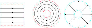
Figure 3. Three fundamental domains: left invariant flow box, middle periodic annulus, right transverse annulus.

Theorem B.

Each connected component of $S-\mathop{\mathrm{BD}}_{0}(v)$ for a regular-like flow $v$ on a compact surface $S$ is one of the following five invariant open subsets exclusively:
$(1)$ A flow box in $\mathrm{P}(v)$,
$(2)$ An annulus in $\mathrm{P}(v)$,
$(3)$ An annulus in $\mathop{\mathrm{Per}}(v)$,
$(4)$ A torus in $\mathop{\mathrm{Per}}(v)$,
$(5)$ An essential subset in $\mathrm{LD}(v)$.

Moreover, if $v$ is of finite-like type, then the union $\mathop{\mathrm{BD}}_{0}(v_{\mathrm{col}})$ is a finite union of singular points, limit cycles, one-sided periodic orbits, and orbits from or to singular points.

A more general result holds for flows of weakly finite-like type (see Theorem 7.7). As mentioned, the Markus-Neumann theorem is not true even for a toral flow which consists of one singular point and non-recurrent orbits. However, we show that the Markus-Neumann theorem is true in a large class, which contains Morse-Smale flows and generic Hamiltonian flows on compact surfaces, under mild conditions. In other words, using the decompositions, we construct a finite complete invariant of a flow of finite type and show the following completeness.

Theorem C.

The orbit complex is a complete invariant for a flow of finite type on an orientable compact surface if either the orbit complexes are equipped with two circuit orders $\leq_{\partial_{\perp}^{\alpha}}$ and $\leq_{\partial_{\perp}^{\omega}}$ or each multi-saddle connection is self-connected.

The present paper consists of ten sections. In the next section, as preliminaries, we introduce some fundamental notions. In §3, the properties of surface flows are described. In particular the non-trivial circuits are studied. In §4, we describe borders between different kinds of orbits to construct decompositions of flows. In §5, decompositions of quasi-regular flows and of flows of finite type are constructed. In particular, Theorem A and Theorem B are proved. In §6, using the decompositions, we enumerate the set of finite type on compact surfaces. In §7, we extend results in §5–6 to those for flows of weakly finite(-like) type. In §8, a finite complete invariant for surface flows of finite type is constructed explicitly. In §9, we show that the Markus-Neumann theorem is true in a large class, which contains Morse-Smale flows and generic Hamiltonian flows on compact surfaces, under mild conditions. In particular, Theorem C is proved. In the final section, we briefly remark on a concrete representation of the finite complete invariant for surface flows of finite type.

2. Preliminaries

2.1. Topological notion

Let $A$ be a subset $A$ of a topological space $X$. Denoted by $\overline{A}$ the closure of $A$, by $\mathrm{int}A$ the interior of $A$, and by $\partial A:=\overline{A}-\mathrm{int}A$ the boundary of $A$. We define the border $\partial^{-}A$ by $A-\mathrm{int}A$ of a subset $A\subseteq X$. Denote by $\partial^{+}A:=\overline{A}-A$ the coborder of a subset $A\subseteq X$. Then $\partial A=\partial^{-}A\sqcup\partial^{+}A$.

2.1.1. $T_{0}$ separation axiom

A point $x$ of a topological space $X$ is $T_{0}$ (or Kolmogorov) if for any point $y\neq x\in X$ there is an open subset $U$ of $X$ such that $|\{x,y\}\cap U|=1$, where $|A|$ is the cardinality of a subset $A$. A topological space is $T_{0}$ if each point is $T_{0}$.

2.1.2. $T_{0}$-tification

By a decomposition, we mean a family $\mathcal{F}$ of pairwise disjoint nonempty subsets of a set $X$ such that $X=\bigsqcup\mathcal{F}$, where $\bigsqcup$ denotes a disjoint union. For a topological space $X$, define the class $\hat{x}:=\{y\in X\mid\overline{\{x\}}=\overline{\{y\}}\}$ for any point $x$ and a decomposition $\hat{X}:=\{\hat{z}\mid z\in X\}$ of classes. Then the decomposition $\hat{X}$ is a $T_{0}$ space as a quotient space, which is called the $T_{0}$-tification (or Kolmogorov quotient) of $X$.

2.1.3. Dimensions

By dimension, we mean Lebesgue covering dimension on a topological space. From Urysohn’s theorem, the Lebesgue covering dimension, the large inductive dimension, and the small inductive dimension correspond in separable metrizable spaces. A compact metrizable space $X$ whose small inductive dimension is $n>0$ is an $n$-dimensional Cantor manifold [42] if the complement $X-L$ for any closed subset $L$ of $X$ whose small inductive dimension is less than $n-1$ is connected. It is known that a compact connected manifold is a Cantor manifold [12, 41, 42] (cf. p.93. Example VI 11 [13]).

2.1.4. Curves and loops

Recall that a curve is a continuous mapping $C:I\to X$ where $I$ is a non-degenerate connected subset of a circle $\mathbb{S}^{1}$. A curve is simple if it is injective. We also denote by $C$ the image of a curve $C$. Denote by $\partial C:=C(\partial I)$ the boundary of a curve $C$, where $\partial I$ is the boundary of $I\subset\mathbb{S}^{1}$. Put $\mathrm{int}C:=C\setminus\partial C$. A simple curve is a simple closed curve if its domain is $\mathbb{S}^{1}$ (i.e. $I=\mathbb{S}^{1}$). A simple closed curve is also called a loop. An arc is a simple curve whose domain is an interval. An orbit arc is an arc contained in an orbit. A maximal orbit arc is an orbit arc which is maximal with respect to the inclusion order. An orbit curve is either an orbit arc or a periodic orbit.

2.1.5. Essential subsets

Recall that a one-dimensional cell complex $\gamma$ is essential in a compact surface $S$ if and only if $\gamma$ is not null homotopic in $S^{*}$, where $S^{*}$ is the resulting surface from $S$ by collapsing all boundary components into singletons. Here a singleton is a set consisting of a point. We call that a subset of a surface $S$ is essential if it is not null homotopic in the resulting surface $S^{*}$ from $S$ by collapsing all boundary components into singletons.

2.2. Notion of dynamical systems

A flow is a continuous $\mathbb{R}$-action on a topological space. Let $v:\mathbb{R}\times X\to X$ be a flow on a topological space $X$. For $t\in\mathbb{R}$, define $v_{t}:X\to X$ by $v_{t}:=v(t,\cdot)$. For a point $x$ of $X$, we denote by $O(x)$ the orbit of $x$, $O^{+}(x)$ the positive orbit (i.e. $O^{+}(x):=\{v_{t}(x)\mid t>0\}$), and $O^{-}(x)$ the negative orbit (i.e. $O^{-}(x):=\{v_{t}(x)\mid t<0\}$). Recall that a point $x$ of $X$ is singular if $x=v_{t}(x)$ for any $t\in\mathbb{R}$, and is periodic if there is a positive number $T>0$ such that $x=v_{T}(x)$ and $x\neq v_{t}(x)$ for any $t\in(0,T)$. A point is closed if it is either singular or periodic. An orbit is singular (resp. periodic, closed) if it contains a singular (resp. periodic, closed) point. Denote by $\mathop{\mathrm{Sing}}(v)$ the set of singular points and by $\mathop{\mathrm{Per}}(v)$ (resp. $\mathop{\mathrm{Cl}}(v)$) the union of periodic (resp. closed) orbits. A point is wandering if there are its neighborhood $U$ and a positive number $N$ such that $v_{t}(U)\cap U=\emptyset$ for any $t>N$. Such $U$ is called a wandering domain. A point is non-wandering if it is not wandering (i.e. for any its neighborhood $U$ and for any positive number $N$, there is a number $t\in\mathbb{R}$ with $|t|>N$ such that $v_{t}(U)\cap U\neq\emptyset$). Denote by $\Omega(v)$ the set of non-wandering points, called the non-wandering set. A flow is non-wandering if the non-wandering set is the whole space.

2.2.1. Topological properties of orbits

An orbit is proper if it is embedded, and locally dense if its closure has a nonempty interior. Denote by $\mathrm{LD}(v)$ (resp. $\mathrm{P}(v)$) the union of locally dense orbits (resp. non-recurrent orbits) for the flow $v$. Note that an orbit on a paracompact manifold is proper if and only if it has a neighborhood in which the orbit is closed [48]. This implies that an orbit on a paracompact manifold is non-closed proper if and only if it is not recurrent. In particular, the union $\mathrm{P}(v)$ for the flow $v$ on a paracompact manifold is the union of non-closed proper orbits.

2.2.2. Limit sets of points and orbits

Recall that the $\omega$-limit (resp. $\alpha$-limit) set of a point $x$ is $\omega(x):=\bigcap_{n\in\mathbb{R}}\overline{\{v_{t}(x)\mid t>n\}}$ (resp. $\alpha(x):=\bigcap_{n\in\mathbb{R}}\overline{\{v_{t}(x)\mid t<n\}}$). For an orbit $O$, define $\omega(O):=\omega(x)$ and $\alpha(O):=\alpha(x)$ for some point $x\in O$. Note that an $\omega$-limit (resp. $\alpha$-limit) set of an orbit is independent of the choice of point in the orbit.

2.2.3. Recurrence and Poisson stability

A point $x$ of $X$ is strongly recurrent (or Poisson stable) if $x\in\omega(x)\cap\alpha(x)$, a point $x$ is positively recurrent (or positively Poisson stable) if $x\in\omega(x)$, a point $x$ is negatively recurrent (or negatively Poisson stable) if $x\in\alpha(x)$, and a point $x$ is recurrent (or positively or negatively Poisson stable) if $x\in\omega(x)\cup\alpha(x)$.

2.2.4. Invariance and saturation

A subset $A$ is positive invariant if $\bigcup_{x\in A}O^{+}(x)\subseteq A$. A subset is invariant (or saturated) if it is a union of orbits. For a closed invariant set $\gamma$, define the stable manifold $W^{s}(\gamma):=\{y\in X\mid\omega(y)\subseteq\gamma\}$ and the unstable manifold $W^{u}(\gamma):=\{y\in X\mid\alpha(y)\subseteq\gamma\}$. The saturation of a subset is the union of orbits intersecting it. Denote by $\mathrm{Sat}_{v}(A)$ or $v(A)$ the saturation of a subset $A$. Then $\mathrm{Sat}_{v}(A)=v(A)=\bigcup_{a\in A}O(a)$.

2.2.5. Orbit classes and quotient spaces of flows

The (orbit) class $\hat{O}$ of an orbit $O$ is the union of orbits each of whose orbit closure corresponds to $\overline{O}$ (i.e. $\hat{O}=\{y\in X\mid\overline{O(y)}=\overline{O}\}$). For a flow $v$ on a topological space $X$, the orbit space $T/v$ (resp. orbit class space $T/\hat{v}$) of an invariant subset $T$ of $X$ is a quotient space $T/\sim$ defined by $x\sim y$ if $O(x)=O(y)$ (resp. $\overline{O(x)}=\overline{O(y)}$). Notice that an orbit space $T/v$ is the set $\{O(x)\mid x\in T\}$ as a set. Moreover, the orbit class space $T/\hat{v}$ is the set $\{\hat{O}(x)\mid x\in T\}$ with the quotient topology. Denote by $\tau_{v}$ (resp. $\tau_{\hat{v}}$) the topology of the orbit space $X/v$ (resp. orbit class space $X/\hat{v}$). Note that the orbit class space $X/{\hat{v}}$ is the $T_{0}$-tification of the orbit space $X/v$, and that $T/v$ (resp. $T/\hat{v}$) is a subset of the orbit space $X/v$ (resp. orbit class space $X/\hat{v}$).

2.2.6. Separatrices

A separatrix is a non-singular orbit whose $\alpha$-limit or $\omega$-limit set is a singular point. A separatrix is connecting if each of its $\omega$-limit set and $\alpha$-limit sets is a singular point.

2.3. Notion of flows on surfaces

By a surface, we mean a two dimensional paracompact manifold, that dose not need to be orientable. From now on, we suppose that flows are on surfaces unless otherwise stated. Let $v$ be a flow on surface $S$.

2.3.1. Topological properties of orbits

An orbit is exceptional if it is neither proper nor locally dense. Denote by $\mathrm{E}(v)$ the union of exceptional orbits. A point is proper (resp. locally dense, exceptional) if so is its orbit. Since surfaces are paracompact manifolds, the union $\mathrm{P}(v)$ of non-recurrent orbits is the union of non-closed proper orbits and so the union $\mathrm{LD}(v)\sqcup\mathrm{E}(v)$ is the union of non-closed recurrent orbits. Therefore we have a decomposition $S=\mathop{\mathrm{Sing}}(v)\sqcup\mathop{\mathrm{Per}}(v)\sqcup\mathrm{P}(v)\sqcup\mathrm{LD}(v)\sqcup\mathrm{E}(v)$, where $\sqcup$ denotes a disjoint union. By Proposition 2.2 [47] and Proposition 2.3 [47], if $x\in\mathrm{LD}(v)$ (resp. $x\in\mathrm{E}(v)$) then $\hat{O}(x)=\overline{O(x)}\cap\mathrm{LD}(v)=\overline{O(x)}\setminus(\mathop{\mathrm{Sing}}(v)\sqcup\mathrm{P}(v))$ (resp. $\hat{O}(x)=\overline{O(x)}\cap\mathrm{E}(v)=\overline{O(x)}\setminus(\mathop{\mathrm{Sing}}(v)\sqcup\mathrm{P}(v))$).

2.3.2. Q-sets

A quasi-minimal set (or a Q-set for brevity) is defined to be the orbit closure of a non-closed recurrent point. It is known that a total number of Q-sets for $v$ cannot exceed $g$ if $S$ is an orientable surface of genus $g$ [23], and $\frac{p-1}{2}$ if $S$ is a non-orientable surface of genus $p$ [20] (cf. Remark 2 [3]). Therefore the closure $\overline{\mathrm{LD}(v)\sqcup\mathrm{E}(v)}$ is a finite union of Q-sets. A (quasi-)minimal set is exceptional (resp. locally dense) if it is a closure of an orbit intersecting $\mathrm{E}(v)$ (resp. $\mathrm{LD}(v)$). Note that exceptional (quasi-)minimal set is transversely a Cantor set (i.e. there is a small neighborhood $U$ of a recurrent point of the minimal set $\mathcal{M}$ such that $\mathcal{M}\cap U$ is a product of an open interval and a Cantor set) because a Cantor set is characterized as a compact metrizable perfect totally disconnected space.

2.3.3. Canonical local structures

Denote by $I$ an interval which is either $(1,2)$, $(1,2]$, $[1,2)$, or $[1,2]$. Let $\mathbb{D}\subset\mathbb{R}^{2}$ be an oriented flow box on $(0,1)\times I$ whose orbits are of form $(0,1)\times\{t\}$ for some $t\in I$ as on the left of Figure 3, $\mathbb{A}_{+}\subset\mathbb{R}^{2}$ an annulus $\{(x,y)\mid x^{2}+y^{2}\in I\}$ whose orbits are $\{(t\cos\theta,t\sin\theta)\mid\theta\in[0,2\pi]\}$ with anti-clockwise flow direction for some $t\in I$ as on the middle of Figure 3, and $\mathbb{A}_{\widetilde{+}}\subset\mathbb{R}^{2}$ an oriented annulus $\{(x,y)\mid x^{2}+y^{2}\in I\}$ whose orbit curves are $\{(t\cos\theta,t\sin\theta)\mid t\in I\}$ with outward flow direction for some $\theta\in[0,2\pi)$ as on the right of Figure 3. A subset $U$ is a flow box (resp. periodic annulus, transverse annulus) if there are some interval $I\in\{(1,2),(1,2],[1,2),[1,2]\}$ and a homeomorphism $h$ from $U$ to $\mathbb{D}$ (resp. $\mathbb{A}_{+}$, $\mathbb{A}_{\widetilde{+}}$) whose images of any maximal orbit curves are maximal orbit curves and which preserves the orientations of the orbit curves.

2.3.4. Types of singular points

A singular point $x$ on (resp. outside of) the boundary $\partial S$ of a surface $S$ is a $\partial$-sink (resp. sink) if there is a neighborhood $U$ of $x$ such that $\omega(y)=\{x\}$ for any $y\in U$, and is a $\partial$-source (resp. source) if there is a neighborhood $U$ of $x$ such that $\alpha(y)=\{x\}$ for any $y\in U$. A point $x$ is a center if for any its neighborhood $U$, there is an invariant open neighborhood $V\subset U$ of $x$ such that $U-\{x\}$ consists of periodic orbits, where $A-B$ is used instead of $A\setminus B$ when $A\subseteq B$. A $\partial$-$k$-saddle (resp. $k$-saddle) is an isolated singular point on (resp. outside of) $\partial S$ with exactly $(2k+2)$-separatrices, counted with multiplicity as in Figure 4.

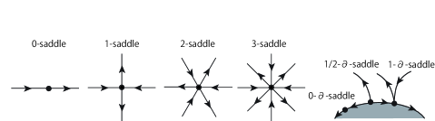
Figure 4. Examples of multi-saddles

In other words, A $\partial$-$k/2$-saddle (resp. $k$-saddle) is an isolated singular point on (resp. outside of) $\partial S$ with exactly $k+1$ (resp. $(2k+2)$) hyperbolic sectors. Here a hyperbolic sector is a local structure as in Figure 5.

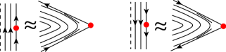
Figure 5. A hyperbolic sector with anti-clockwise flow direction and a hyperbolic sector with clockwise flow direction

A multi-saddle is a $k$-saddle or a $\partial$-$(k/2)$-saddle for some $k\in\mathbb{Z}_{\geq 0}$. A $1$-saddle is topologically an ordinary saddle and a $\partial$-$(1/2)$-saddle is topologically a $\partial$-saddle. A separatrix is semi-multi-saddle if it is from or to a multi-saddle. A connecting separatrix is a saddle (resp. multi-saddle) separatrix if its $\alpha$-limit and $\omega$-limit set are saddles and $\partial$-saddles (resp. multi-saddles).

2.3.5. (Multi-)saddle connection diagrams

The saddle (resp. multi-saddle) connection diagram $D(v)$ is the union of saddles (resp. multi-saddles) and saddle (resp. multi-saddle) separatrices. A saddle (resp. multi-saddle) connection is a connected component of the saddle (resp. multi-saddle) connection diagram. Note that a multi-saddle connection is also called a poly-cycle.

2.3.6. Self-connectedness

A multi-saddle separatrix is self-connected if either its $\omega$-limit set and $\alpha$-limit set correspond or it connects multi-saddles on the same boundary component. Note that a homoclinic multi-saddle separatrix is self-connected and a heteroclinic multi-saddle separatrix outside of the boundary is not self-connected. A (multi-)saddle connection is self-connected if all the separatrices are self-connected. The (multi-)saddle connection diagram is self-connected if so is each connected component.

2.3.7. (Quasi-)Regularity

A flow is quasi-regular if each singular point is either a center, a multi-saddle, a sink, a $\partial$-sink, a source, or a $\partial$-source. Note that a non-wandering flow with finitely many singular points on a compact surface is quasi-regular (see Theorem 3 [7]). Conversely, a quasi-regular flow on a compact surface has finitely many singular points.

2.3.8. Collars

Recall that an annular subset is homeomorphic to an annulus. An open annular subset $\mathbb{A}$ of a surface is a collar of an invariant subset $\gamma$ if there is an open connected neighborhood $U$ of $\gamma$ such that $\mathbb{A}$ is a connected component of the complement $U-\gamma$. Note that an open annular subset $\mathbb{A}$ of a surface is a collar of a singular point $x$ if and only if the union $\mathbb{A}\sqcup\{x\}$ is an open disk and a neighborhood of $x$.

2.3.9. Circuits

A trivial circuit is a singular point. A trivial circuit $x$ is semi-attracting (resp. semi-repelling) if there is its collar which is contained in the stable (resp. unstable) manifold of $x$. In other words, a semi-attracting trivial circuit is either a $\partial$-source or a source, and a semi-repelling trivial circuit is either a $\partial$-sink or a sink. By a cycle or a periodic circuit, we mean a periodic orbit. By a non-trivial circuit, we mean either a cycle or a continuous image of a circle which is a graph but not a singleton and which is the union of separatrices and finitely many singular points. Note that a non-trivial circuit is not a local injection in general (see Figure 6). Here a mapping is a local injection if for any point in a domain there is its neighborhood to which the restriction is injection.

Figure 6. A degenerate singular point with infinitely many connecting separatrices

A circuit is either a trivial or non-trivial circuit. Note that there are circuits with infinitely many edges and that any non-trivial non-periodic circuit contains non-recurrent orbits as in Figure 6. A non-trivial circuit is a multi-saddle circuit if it is contained in a multi-saddle connection. Recall that a boundary component of a subset $A$ is a connected component of the boundary of $A$. A non-trivial circuit $\gamma$ is a limit circuit if there is a point $x\notin\gamma$ with $\omega(x)=\gamma$ or $\alpha(x)=\gamma$. A limit cycle is a limit circuit in $\mathop{\mathrm{Per}}(v)$. A circuit $\gamma$ is a semi-attracting (resp. semi-repelling) circuit with respect to a small collar $\mathbb{A}$ if $\omega(x)=\gamma$ (resp. $\alpha(x)=\gamma$) and $O^{+}(x)\subset\mathbb{A}$ (resp. $O^{-}(x)\subset\mathbb{A}$) for any point $x\in\mathbb{A}$. Then $\mathbb{A}$ is called a semi-attracting (resp. a semi-repelling) collar basin of $\gamma$.

2.3.10. Flows of finite type

A flow is of finite type if (1) it is quasi-regular, (2) there are at most finitely many limit cycles, and (3) $\mathrm{LD}(v)\sqcup\mathrm{E}(v)=\emptyset$ $(\mathrm{i.e.}$ Any recurrent orbits are closed$)$.

2.3.11. One- and two-sided circuits

A non-trivial circuit $\gamma$ is one-sided if for any small neighborhood $U$ of $\gamma$ there is a collar $V\subset U$ of $\gamma$ such that the union $V\sqcup\gamma$ is a neighborhood of some point in $\mathrm{P}(v)\cap\gamma$. A non-trivial circuit $\gamma$ is two-sided if it is not one-sided (i.e. there is a small neighborhood $U$ of $\gamma$ such that the union $V\sqcup\gamma$ for any collar $V\subset U$ of $\gamma$ is not a neighborhood of any point in $\mathrm{P}(v)\cap\gamma$. For a circuit $\mu$ which is a simple closed curve, notice that the circuit $\mu$ is one-sided if and only if it is either a boundary component of a surface or has a small neighborhood which is a Möbius band, and that the circuit $\mu$ is two-sided if and only if it has an open small annular neighborhood $\mathbb{A}$ such that the complement $\mathbb{A}-\mu$ consists of two open annuli.

2.3.12. Ss-multi-saddle connection diagrams

An invariant subset is called an ss-component if it is either a sink, a $\partial$-sink, a source, a $\partial$-source, a limit circuit, or an exceptional Q-set. In other words, an invariant subset is called an ss-component if and only if it is either a semi-attracting/semi-repelling circuit or an exceptional Q-set. A semi-multi-saddle separatrix is an ss-separatrix if it connects a multi-saddle and an ss-component. In other words, a semi-multi-saddle separatrix is an ss-separatrix if its $\alpha$-limit or $\omega$-limit set is an ss-component. The ss-multi-saddle connection diagram $D_{\mathrm{ss}}(v)$ is the union of multi-saddles, multi-saddle separatrices, ss-separatrices, and ss-components. An ss-multi-saddle connection is a connected component of the ss-multi-saddle connection diagram. Note that $D_{\mathrm{ss}}(v)$ is the union of the multi-saddle connection diagram, ss-separatrices, and ss-components.

2.3.13. Border points

Denote by $\partial_{\mathop{\mathrm{Per}}(v)}$ the union of periodic orbits in an intersection $\partial S\cap\mathrm{int}\mathop{\mathrm{Per}}(v)$. Moreover, denote by $\mathop{\mathrm{P}_{\mathrm{ms}}}(v)$ (resp. $\mathop{\mathrm{P}_{\mathrm{ss}}}(v)$) the union of multi-saddle separatrices (resp. ss-separatrices) in $\mathrm{int}\mathrm{P}(v)$. Define $\mathrm{P}_{\mathrm{lc}}(v):=\bigcup\{\gamma\subset\mathrm{int}\mathrm{P}(v)\sqcup\mathop{\mathrm{Sing}}(v):\text{limit circuit}\}\setminus\mathop{\mathrm{Sing}}(v)$. In other words, the set $\mathrm{P}_{\mathrm{lc}}(v)$ is the intersection of $\mathrm{int}\mathrm{P}(v)$ and the union of limit circuits. In addition, define $\mathop{\partial_{\mathrm{P}(v)}}$ the union of orbits on $\partial S$ which connect $\partial$-sinks and $\partial$-sources. Note that compactness of $S$ implies that $\mathop{\partial_{\mathrm{P}(v)}}$ is a finite union of non-recurrent orbits on $\partial S\cap\mathrm{int}\mathrm{P}(v)$. Put $\mathop{\mathrm{P}_{\mathrm{sep}}}(v):=(\mathop{\mathrm{P}_{\mathrm{lc}}}(v)\cup\mathop{\mathrm{P}_{\mathrm{ms}}}(v))\sqcup\mathop{\mathrm{P}_{\mathrm{ss}}}(v)\sqcup\mathop{\partial_{\mathrm{P}(v)}}$. We have the following observation.

Lemma 2.1.

The following statements hold for a quasi-regular flow $v$ on a surface $S$:
(1) $\mathrm{P}_{\mathrm{lc}}(v)\subseteq\mathop{\mathrm{P}_{\mathrm{ms}}}(v)$.
(2) The union $\mathop{\mathrm{P}_{\mathrm{ms}}}(v)\sqcup\mathop{\mathrm{P}_{\mathrm{ss}}}(v)$ is the union of semi-multi-saddle separatrices in $\mathrm{int}\mathrm{P}(v)$.
(3) The union $\mathop{\mathrm{P}_{\mathrm{sep}}}(v)=\mathop{\mathrm{P}_{\mathrm{ms}}}(v)\sqcup\mathop{\mathrm{P}_{\mathrm{ss}}}(v)\sqcup\mathop{\partial_{\mathrm{P}(v)}}$ is the union of semi-multi-saddle separatrices in $\mathrm{int}\mathrm{P}(v)$ and non-recurrent orbits on the boundary $\partial S$.

We will show that the union $\partial^{-}\mathrm{P}(v)\sqcup\mathop{\mathrm{P}_{\mathrm{ms}}}(v)\sqcup\mathop{\mathrm{P}_{\mathrm{ss}}}(v)$ is the union of semi-multi-saddle separatrices if $v$ is quasi-regular (see Corollary 4.6). Define the strict border point set $\mathop{\mathrm{Bd}}(v)$ for the flow $v$ as follows:

$$\mathop{\mathrm{Bd}}(v):=\partial\mathop{\mathrm{Sing}}(v)\cup\partial\mathop{\mathrm{Per}}(v)\cup\partial_{\mathop{\mathrm{Per}}(v)}\cup\partial\mathrm{P}(v)\cup\mathop{\mathrm{P}_{\mathrm{sep}}}(v)\cup\partial\mathrm{LD}(v)\cup\partial\mathrm{E}(v)$$

We will prove that $\mathop{\mathrm{Bd}}(v)=\mathop{\mathrm{Sing}}(v)\sqcup\partial^{-}\mathop{\mathrm{Per}}(v)\sqcup\partial_{\mathop{\mathrm{Per}}(v)}\sqcup\partial^{-}\mathrm{P}(v)\sqcup\mathop{\mathrm{P}_{\mathrm{sep}}}(v)\sqcup\mathrm{E}(v)$ if $v$ is a flow with finitely many singular points on a compact surface (see Lemma 4.12). Denote by $\mathop{\mathrm{Per}}_{1}(v)$ the union of one-sided periodic orbits in $\mathrm{int}(\mathop{\mathrm{Per}}(v)-\partial_{\mathop{\mathrm{Per}}(v)})$. Define the border point set $\mathop{\mathrm{BD}}(v):=\mathop{\mathrm{Bd}}(v)\sqcup\mathop{\mathrm{Per}}_{1}(v)$. In other words, we have the following relation:

$$\mathop{\mathrm{BD}}(v)=\partial\mathop{\mathrm{Sing}}(v)\cup\partial\mathop{\mathrm{Per}}(v)\cup\partial_{\mathop{\mathrm{Per}}(v)}\cup\mathop{\mathrm{Per}_{1}}(v)\cup\partial\mathrm{P}(v)\cup\mathop{\mathrm{P}_{\mathrm{sep}}}(v)\cup\partial\mathrm{LD}(v)\cup\partial\mathrm{E}(v)$$

Note that the union $\partial_{\mathop{\mathrm{Per}}(v)}\sqcup\mathop{\mathrm{Per}}_{1}(v)$ is the union of one-sided periodic orbits in $\mathrm{int}\mathop{\mathrm{Per}}(v)$.

2.3.14. Transversality

Notice that we can define transversality using tangential spaces of surfaces because each flow on a compact surface is topologically equivalent to a $C^{1}$-flow by the Gutierrez’s smoothing theorem [10]. However, to modify transverse arcs explicitly, we define immediately transversality as follows. A curve $C$ is transverse to $v$ at a point $p\in\mathrm{int}C$ if there are a small neighborhood $U$ of $p$ and a homeomorphism $h:U\to[-1,1]^{2}$ with $h(p)=0$ such that $h^{-1}([-1,1]\times\{t\})$ for any $t\in[-1,1]$ is an orbit arc and $h^{-1}(\{0\}\times[-1,1])=C\cap U$. A curve $C$ is transverse to $v$ at a point $p\in\partial C\cap\partial S$ (resp. $p\in\partial C\setminus\partial S$) if there are a small neighborhood $U$ of $p$ and a homeomorphism $h:U\to[-1,1]\times[0,1]$ (resp. $h:U\to[-1,1]^{2}$) with $h(p)=0$ such that $h^{-1}([-1,1]\times\{t\})$ for any $t\in[0,1]$ (resp. $t\in[-1,1]$) is an orbit arc and $h^{-1}(\{0\}\times[0,1])=C\cap U$ (resp. $h^{-1}(\{0\}\times[-1,1])=C\cap U$).

A simple curve $C$ is transverse to $v$ if so is it at any point in $C$. A simple curve $C$ is transverse to $v$ is called a transverse arc. A simple closed curve is a closed transversal if it transverses to $v$.

3. Properties of surface flows

Let $v$ be a flow on a compact connected surface $S$. We state the inherited properties for double covers.

Lemma 3.1.

Let $v$ be a flow on a compact surface $S$ and $p\colon\widetilde{S}\to S$ a double cover. Then the following statement holds for any point $x\in S$:
$(1)$ Either $\hat{O}(x_{+})=\hat{O}(x_{-})=p^{-1}(\hat{O}(x))$ or $\hat{O}(x_{+})\sqcup\hat{O}(x_{-})=p^{-1}(\hat{O}(x))$
$(2)$ $p^{-1}(\mathop{\mathrm{Sing}}(v))=\mathop{\mathrm{Sing}}(\widetilde{v})$
$(3)$ $p^{-1}(\mathop{\mathrm{Per}}(v))=\mathop{\mathrm{Per}}(\widetilde{v})$
$(4)$ $p^{-1}(\mathrm{P}(v))=\mathrm{P}(\widetilde{v})$
$(5)$ $p^{-1}(\mathrm{LD}(v))=\mathrm{LD}(\widetilde{v})$
$(6)$ $p^{-1}(\mathrm{E}(v))=\mathrm{E}(\widetilde{v})$

Proof.

By the Gutierrez’s smoothing theorem [10], the flow is generated by a vector field up to topological equivalence. Notice that any flow generated by a vector field $X$ on a connected compact manifold induces the induced flow on the finite cover because $X$ can be lifted to the cover. Let $\widetilde{v}$ be the lift of $v$ on a double cover $\widetilde{S}$ of $S$. For a point $x\in S$, put $\{x_{+},x_{-}\}:=p^{-1}(x)$. For $A\subseteq S$, since covering maps are locally homeomorphisms, we have $p^{-1}(A)=\{x_{+},x_{-}\mid x\in A\}$ and so $\overline{p^{-1}(A)}=p^{-1}(\overline{A})=\{x_{+},x_{-}\mid x\in\overline{A}\}$. Suppose that $x\in\mathop{\mathrm{Sing}}(v)\sqcup\mathop{\mathrm{Per}}(v)$. Then the lift $p^{-1}(O(x))$ consists of one or two closed orbits of $\widetilde{v}$ and so of one or two orbit classes. Since lifts of singular (resp. periodic, non-closed) points are singular (resp. periodic, non-closed), the assertions $(2)$ and $(3)$ hold. Moreover, the assertion $(1)$ for closed points holds. Thus we may assume that $x\in\mathrm{P}(v)\sqcup\mathrm{LD}(v)\sqcup\mathrm{E}(v)$. Since the non-recurrence is invariant under taking finite coverings, we have that $x\in\mathrm{P}(v)$ if and only if $p^{-1}(x)\subseteq\mathrm{P}(\widetilde{v})$. This means that the assertion $(4)$ holds. Moreover, if $x\in\mathrm{P}(v)$, then either $O(x_{+})=O(x_{-})=\hat{O}(x_{+})=\hat{O}(x_{-})=p^{-1}(\hat{O}(x))=p^{-1}(O(x))$ or $O(x_{+})\sqcup O(x_{-})=\hat{O}(x_{+})\sqcup\hat{O}(x_{-})=p^{-1}(\hat{O}(x))=p^{-1}(O(x))$. This implies that the assertion $(1)$ for non-recurrent points holds. The assertions $(2)$–$(4)$ imply that $p^{-1}(\mathrm{LD}(v)\sqcup\mathrm{E}(v))=\mathrm{LD}(\widetilde{v})\sqcup\mathrm{E}(\widetilde{v})$. Thus we may assume that $x\in\mathrm{LD}(v)\sqcup\mathrm{E}(v)$. Then $p^{-1}(x)\subseteq\mathrm{LD}(\widetilde{v})\sqcup\mathrm{E}(\widetilde{v})$. Proposition 2.2 [47] implies that $\hat{O}(x)=\overline{O(x)}\setminus(\mathop{\mathrm{Sing}}(v)\sqcup\mathrm{P}(v))=\overline{O(x)}\cap(\mathrm{LD}(v)\sqcup\mathrm{E}(v))$, $\hat{O}(x_{+})=\overline{O(x_{+})}\setminus(\mathop{\mathrm{Sing}}(\widetilde{v})\sqcup\mathrm{P}(\widetilde{v}))=\overline{O(x_{+})}\cap(\mathrm{LD}(\widetilde{v})\sqcup\mathrm{E}(\widetilde{v}))$, and $\hat{O}(x_{-})=\overline{O(x_{-})}\setminus(\mathop{\mathrm{Sing}}(\widetilde{v})\sqcup\mathrm{P}(\widetilde{v}))=\overline{O(x_{-})}\cap(\mathrm{LD}(\widetilde{v})\sqcup\mathrm{E}(\widetilde{v}))$. Since the cover $p$ is a local homeomorphism, we have that $\hat{O}(x_{+})\cup\hat{O}(x_{-})\subseteq p^{-1}(\hat{O}(x))=p^{-1}(\overline{O(x)}\cap(\mathrm{LD}(v)\sqcup\mathrm{E}(v)))\subseteq p^{-1}(\overline{O(x)})\cap p^{-1}((\mathrm{LD}(v)\sqcup\mathrm{E}(v)))=\overline{p^{-1}(O(x))}\cap(\mathrm{LD}(\widetilde{v})\sqcup\mathrm{E}(\widetilde{v}))=\overline{O(x_{-})\cup O(x_{+})}\cap(\mathrm{LD}(\widetilde{v})\sqcup\mathrm{E}(\widetilde{v}))=(\overline{O(x_{-})}\cup\overline{O(x_{+})})\cap(\mathrm{LD}(\widetilde{v})\sqcup\mathrm{E}(\widetilde{v}))=\hat{O}(x_{+})\cup\hat{O}(x_{-})$. This implies the assertion $(1)$. Suppose that $\hat{O}(x_{+})=\hat{O}(x_{-})$. Then $p^{-1}(\hat{O}(x))=\hat{O}(x_{+})=\hat{O}(x_{-})\subseteq\mathrm{LD}(\widetilde{v})\sqcup\mathrm{E}(\widetilde{v})$ and $p^{-1}(\overline{O(x)})=\overline{p^{-1}(O(x))}=\overline{O(x_{+})}=\overline{O(x_{-})}$. The local homeomorphic property of the covering map $p$ implies that $\mathrm{int}\,\overline{O(x)}\neq\emptyset$ if and only if $\mathrm{int}\,\overline{O(x_{+})}=\mathrm{int}\,\overline{O(x_{-})}\neq\emptyset$. Hence the assertion $(6)$ holds. Since $\mathrm{E}(v)=S-(\mathop{\mathrm{Sing}}(v)\sqcup\mathop{\mathrm{Per}}(v)\sqcup\mathrm{P}(v)\sqcup\mathrm{LD}(v))$, the assertions $(2)$–$(5)$ implies the assertion $(6)$. Thus we may assume that $\hat{O}(x_{+})\neq\hat{O}(x_{-})$. Then $p^{-1}(\hat{O}(x))=\hat{O}(x_{+})\sqcup\hat{O}(x_{-})\subseteq\mathrm{LD}(\widetilde{v})\sqcup\mathrm{E}(\widetilde{v})$, $x_{+}\notin\overline{O(x_{-})}$, and $x_{-}\notin\overline{O(x_{+})}$. Since the complement $S-\overline{O(x_{-})}$ is an invariant open neighborhood of $x_{+}$, the local homeomorphic property of the covering map $p$ and the homogeneity of orbits imply that $\mathrm{int}\,\overline{O(x)}\neq\emptyset$ if and only if $\mathrm{int}\,\overline{O(x_{+})}\neq\emptyset$. Similarly, we have that $\mathrm{int}\,\overline{O(x)}\neq\emptyset$ if and only if $\mathrm{int}\,\overline{O(x_{-})}\neq\emptyset$. This implies the assertion $(5)$ holds. Since $\mathrm{E}(v)=S-(\mathop{\mathrm{Sing}}(v)\sqcup\mathop{\mathrm{Per}}(v)\sqcup\mathrm{P}(v)\sqcup\mathrm{LD}(v))$, the assertions $(2)$–$(5)$ implies the assertion $(6)$. ∎

Recall that $\partial^{-}A=A-\mathrm{int}A$ and $\partial^{+}A=\overline{A}-A$ for a subset $A\subseteq S$. Note that the closedness of the singular point set implies $\partial^{-}\mathrm{P}(v)=\mathrm{P}(v)-\mathrm{int}\mathrm{P}(v)=\mathrm{P}(v)\cap\overline{\mathop{\mathrm{Sing}}(v)\sqcup\mathop{\mathrm{Per}}(v)\sqcup\mathrm{LD}(v)\sqcup\mathrm{E}(v)}=\mathrm{P}(v)\cap\overline{\mathop{\mathrm{Per}}(v)\sqcup\mathrm{LD}(v)\sqcup\mathrm{E}(v)}=\mathrm{P}(v)\cap(\partial^{+}\mathop{\mathrm{Per}}(v)\cup\partial^{+}\mathrm{LD}(v)\cup\partial^{+}\mathrm{E}(v))$. We have the following inclusion relations.

Lemma 3.2.

The following statements hold for a flow $v$ on a compact surface $S$:
$(1)$ $\partial^{+}\mathrm{LD}(v)\subseteq\partial^{-}\mathop{\mathrm{Sing}}(v)\sqcup\partial^{-}\mathrm{P}(v)$.
$(2)$ $\partial^{+}\mathrm{E}(v)\subseteq\partial^{-}\mathop{\mathrm{Sing}}(v)\sqcup\partial^{-}\mathrm{P}(v)$.
$(3)$ $\partial^{+}\mathop{\mathrm{Per}}(v)\subseteq\partial^{-}\mathop{\mathrm{Sing}}(v)\sqcup\partial^{-}\mathrm{P}(v)$.
$(4)$ $\partial^{+}\mathop{\mathrm{Sing}}(v)=\emptyset$.
$(5)$ $\partial^{+}\mathrm{P}(v)\subseteq\partial^{-}\mathop{\mathrm{Sing}}(v)\sqcup\partial^{-}\mathop{\mathrm{Per}}(v)\sqcup\partial^{-}\mathrm{LD}(v)\sqcup\partial^{-}\mathrm{E}(v)$.

In particular, we have $\partial^{+}\mathop{\mathrm{Per}}(v)\cup\partial^{+}\mathrm{LD}(v)\cup\partial^{+}\mathrm{E}(v)\subseteq\partial^{-}\mathop{\mathrm{Sing}}(v)\sqcup\partial^{-}\mathrm{P}(v)$.

Proof.

As mentioned, it is known that a total number of Q-sets for $v$ is bounded [20, 23]. By Proposition 2.2 [47], the assertions $(1)$ and $(2)$ hold. Lemma 2.3 [47] implies that $\overline{\mathop{\mathrm{Per}}(v)}\cap(\mathrm{LD}(v)\sqcup\mathrm{E}(v))=\emptyset$ and so $\overline{\mathop{\mathrm{Per}}(v)}\subseteq\partial^{-}\mathop{\mathrm{Sing}}(v)\sqcup\mathop{\mathrm{Per}}(v)\sqcup\partial^{-}\mathrm{P}(v)$. The closedness of the singular point set $\mathop{\mathrm{Sing}}(v)$ implies $\partial^{+}\mathop{\mathrm{Sing}}(v)=\emptyset$. By definition of $\partial^{+}$, the assertion $(5)$ holds. ∎

We obtain the following description of a neighborhood of $\mathop{\mathrm{Per}}(v)$.

Lemma 3.3.

The union $\mathop{\mathrm{Per}}(v)\sqcup\mathrm{int}\mathrm{P}(v)$ is an open neighborhood of $\mathop{\mathrm{Per}}(v)$. In particular, $\mathop{\mathrm{Per}}(v)\cap\overline{\partial^{-}\mathrm{P}(v)}=\emptyset$.

Proof.

By Lemma 3.1, taking the orientation double covering and the double of the surface $S$ if necessary, we may assume that $S$ is closed and orientable. Fix a point $x\in\mathop{\mathrm{Per}}(v)$. Take a small collar $U\subseteq S-\mathop{\mathrm{Sing}}(v)$ of $O(x)$. The flow box theorem (cf. Theorem 1.1, p.45[4]) implies that there are an open annulus $\mathbb{A}\subseteq U$ which is also a collar of $O(x)$ and a transverse closed arc $T_{+}\subseteq\overline{\mathbb{A}}$ such that $x$ is contained in $\partial T_{+}$. Then there are a small subinterval $S_{+}\subseteq T_{+}$ containing $x$ and the first return map $f_{v+}:S_{+}\to T_{+}$ induced by $v$. Then $f_{v+}(x)=x$. Identify $T_{+}$ with $[0,1]$ (resp. $x$ with $0$).

We show that $\mathrm{Sat}_{v}(T_{+})\subseteq\mathop{\mathrm{Per}}(v)\sqcup\mathrm{int}\mathrm{P}(v)$. Indeed, suppose that $f_{v+}:S_{+}\to T_{+}$ is either attracting or repelling near zero. Then $O$ is a limit cycle and so $\mathrm{Sat}_{v}(T_{+})\subseteq\mathop{\mathrm{Per}}(v)\sqcup\mathrm{int}\mathrm{P}(v)$. Suppose that $f_{v+}:S_{+}\to T_{+}$ is neither attracting nor repelling near zero. This implies that zero is an accumulation point of the fixed point set $\mathop{\mathrm{Fix}}(f_{v+})$. Shortening $T_{+}$, we may assume that $f_{v+}(1)=1$ and so $S_{+}=T_{+}$. Then the saturation of $T_{+}$ is a closed annulus, and each orbit intersecting $\mathrm{Fix}(f_{v+})$ is contained in $\mathop{\mathrm{Per}}(v)$ and each orbit intersecting $T_{+}-\mathrm{Fix}(f_{v})$ is contained in $\mathrm{int}\mathrm{P}(v)$. Therefore $\mathrm{Sat}_{v}(T_{+})\subseteq\mathop{\mathrm{Per}}(v)\sqcup\mathrm{int}\mathrm{P}(v)$.

By symmetry, there is a transverse closed arc $T_{-}\subseteq\overline{\mathbb{A}}$ with $x\in\partial T_{-}$ such that $T_{-}\cap U=\emptyset$ and $\mathrm{Sat}_{v}(T_{+})\subseteq\mathrm{int}(\mathop{\mathrm{Per}}(v)\sqcup\mathrm{int}\mathrm{P}(v))$. Then the union $T:=T_{-}\cup T_{+}$ is a transverse closed arc with $x\in\mathrm{int}T$ such that $\mathrm{Sat}_{v}(T)\subseteq\mathrm{int}(\mathop{\mathrm{Per}}(v)\sqcup\mathrm{int}\mathrm{P}(v))$. This implies that $\mathop{\mathrm{Per}}(v)\sqcup\mathrm{int}\mathrm{P}(v)$ is a neighborhood of $x$ and so of $\mathop{\mathrm{Per}}(v)$. In addition, since $(\mathop{\mathrm{Per}}(v)\sqcup\mathrm{int}\mathrm{P}(v))\cap\partial^{-}\mathrm{P}(v)=\emptyset$, the openness implies that $\mathop{\mathrm{Per}}(v)\cap\overline{\partial^{-}\mathrm{P}(v)}\subseteq\mathrm{int}(\mathop{\mathrm{Per}}(v)\sqcup\mathrm{int}\mathrm{P}(v))\cap\overline{\partial^{-}\mathrm{P}(v)}=\emptyset$. ∎

We describe the border of $\mathop{\mathrm{Per}}(v)$.

Lemma 3.4.

The border $\partial^{-}\mathop{\mathrm{Per}}(v)\subseteq\overline{\mathrm{int}\mathrm{P}(v)}$ is contained in the closure of the union of limit cycles.

Proof.

Obviously, each limit cycle is contained in $\partial^{-}\mathop{\mathrm{Per}}(v)$. Therefore the closure of the union of limit cycles is contained in $\partial^{-}\mathop{\mathrm{Per}}(v)$. From Lemma 3.3, the union $\mathop{\mathrm{Per}}(v)\sqcup\mathrm{int}\mathrm{P}(v)$ is an open neighborhood of $\mathop{\mathrm{Per}}(v)$. Then $\partial^{-}\mathop{\mathrm{Per}}(v)\subset\overline{\mathrm{int}\mathrm{P}(v)}$. By Lemma 3.1, taking the orientation double covering if necessary, we may assume that $S$ is orientable. Fix a periodic orbit $O\subseteq\partial^{-}\mathop{\mathrm{Per}}(v)$. If $O$ is a limit cycle, then $O\subseteq\overline{\mathrm{int}\mathrm{P}(v)}$. Thus we may assume that $O$ is not a limit cycle. Since $O\cap\mathrm{int}\mathop{\mathrm{Per}}(v)=\emptyset$, it has a collar $U$ which is contained in $\mathop{\mathrm{Per}}(v)\sqcup\mathrm{int}\mathrm{P}(v)$ such that $O\subseteq\overline{U}$. The flow box theorem implies that there are an open annulus $\mathbb{A}\subseteq U$ and a transverse closed arc $T\subseteq\overline{\mathbb{A}}$ such that $\mathbb{A}$ is a collar of $O$ and $O\cap T$ is contained in $\partial T$. Identify $T$ with $[0,1]$ (resp. $O\cap T$ with $0$). Then there are a small subinterval $S\subseteq T$ containing $x$ and the first return map $f_{v}:S\to T$ induced by $v$. Then $f_{v}(0)=0$. The fact $O\subset\overline{\mathrm{int}\mathrm{P}(v)}$ implies that the first return map $f_{v}$ is not identical. Since $O$ is not a limit cycle, the return map $f_{v}:S\to T$ is neither attracting nor repelling near zero. This implies that zero is an accumulation point of the fixed point set $\mathop{\mathrm{Fix}}(f_{v})$. Since $O\subseteq\overline{\mathrm{int}\mathrm{P}(v)}$, the transverse $T$ has a convergence sequence to zero of fixed points which are either attracting or repelling from at least one side. This means that $O$ is contained in the closure of the union of limit cycles. ∎

We describe the existence of closed transversals.

Lemma 3.5.

Let $I$ be a transverse arc and $x\in I$ such that $|I\cap O(x)|=\infty$. Then there are an orbit arc $C$ in $O(x)$ and a transverse closed arc $J\subseteq I$ such that the union $\mu:=J\cup C$ is a loop with $C\cap J=\partial C=\partial J$ and that the return map along $C$ is orientation-preserving between neighborhoods of $\partial C$ in $I$. Moreover, there is a closed transversal $\gamma$ intersecting $O(x)$ arbitrarily near $\mu$.

Proof.

By time reversion if necessary, we may assume that $O^{+}(x)\cap\mathrm{int}I=\infty$. Fix a point $x_{0}\in O^{+}(x)\cap\mathrm{int}I$. Let $f_{v}:I\to I$ be the first return map on $I$ induced by $v$, $x_{i}:=(f_{v})^{i}(x_{0})$ the $i$-th return of $x_{0}$. For any points $a,b\in I$, denote by $C_{a,b}\subset O^{+}(x)$ the orbit arc from $a$ to $b$ and by $I_{a,b}\subset I$ the subinterval between $a$ and $b$ of $I$. We may assume that $x_{0}<x_{1}$. If the restriction of $f_{v}$ to a neighborhood of $x_{0}$ is orientation-preserving, then the first return map along the orbit arc $C_{x_{0},x_{1}}$ is desired. Thus we may assume that the restriction of $f_{v}$ to a neighborhood of $x_{i}$ for any $i\in\mathbb{Z}_{\geq 0}$ is orientation-reversing. Suppose that $x_{2}<x_{1}$. Since the first return map along $C_{x_{1},x_{2}}$ is orientation-reversing, the first return map for $I_{x_{2},x_{0}}$ along $C_{x_{0},x_{2}}$ is orientation-preserving such that a pair of $C:=C_{x_{0},x_{2}}$ and $J:=I_{x_{2},x_{0}}$ is desired. Thus we may assume that suppose that $x_{i}<x_{i+1}$ for any $i\in\mathbb{Z}_{\geq 0}$. Then each pair of loops $\gamma_{i}:=C_{x_{2i},x_{2i+1}}\cup I_{x_{2i+1},x_{2i}}$ has disjoint neighborhoods each of which is a Möbius band. This means that $S$ has infinitely many non-orientable genus, which contradicts the compactness of $S$.

Moreover, by the waterfall construction to the loop $\mu$ (see Figure 7), there is a closed transversal $\gamma$ intersecting $O(x)$ arbitrarily near $\mu$. ∎

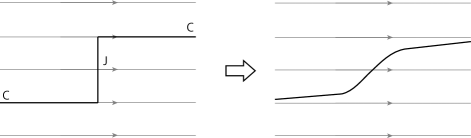
Figure 7. The waterfall construction

We show the existence of a closed transversal with infinitely many intersections for non-closed recurrent orbits.

Lemma 3.6.

For any point $x\in\mathrm{LD}(v)\sqcup\mathrm{E}(v)$, there is a closed transversal $\gamma$ through $O(x)$ such that the intersection $\gamma\cap O(x)$ is infinite. Moreover each closed transversal through a point $y$ in $\mathrm{LD}(v)\sqcup\mathrm{E}(v)$ is essential and intersects $O(y)$ infinitely many times.

Proof.

Fix a point $x\in\mathrm{LD}(v)\sqcup\mathrm{E}(v)$ and a transverse arc $I\subset U$ such that $x$ is the interior point of $I$. Then $|I\cap O(x)|=\infty$. By Lemma 3.5, there are an orbit arc $C$ in $O(x)$ and a transverse closed arc $J\subseteq I$ such that the union $\mu:=J\cup C$ is a loop with $C\cap J=\partial C=\partial J$ and that the return map along $C$ is orientation-preserving between neighborhoods of $\partial C$ in $I$. By the waterfall construction to the loop $\mu$, there is a closed transversal $\gamma$ intersecting $O(x)$ arbitrarily near $\mu$.

Let $\nu$ be a closed transversal through a point $y$ in $\mathrm{LD}(v)\sqcup\mathrm{E}(v)$. Since $y$ is non-closed recurrent, the intersection $\nu\cap O(y)$ is infinite. Suppose that $\nu$ is not essential. Let $S^{*}$ be the resulting closed surface from $S$ by collapsing all boundary components into singletons. Then $\nu$ is null homotopic in $S^{*}$ and so the point $y\in\mathrm{P}(v)$, which contradicts the recurrence of $y$. ∎

We recall the following Maǐer’s result [23] (cf. Theorem 2.4.4 p.32 [29], Theorem 4.2 [3]).

Lemma 3.7 (Maǐer).

Let $v$ be a flow on a compact connected surface $S$. A point $x\in\omega(z)$ for some point $z\in S$ with $\omega(x)\setminus\mathop{\mathrm{Cl}}(v)\neq\emptyset$ is non-closed positively recurrent. In particular, we have $x\in\omega(x)\cap(\mathrm{LD}(v)\sqcup\mathrm{E}(v))$.

The original Maǐer’s Russian paper is not translated. Hence we state a proof of this result which is based on the sketch of a proof of Theorem 4.2 [3].

Proof.

Since $\omega(x)\setminus\mathop{\mathrm{Cl}}(v)\neq\emptyset$, the point $x$ is not closed. Fix a non-closed point $y\in\omega(x)\setminus\mathop{\mathrm{Cl}}(v)$. Then there is a transverse closed arc $I_{[-1,1]}:[-1,1]\to S$ with $y=I_{[-1,1]}(0)$ such that the positive orbit $O^{+}(x)$ intersects $I_{[-1,1]}([-1,0])$ infinitely many times. Denote by $I:=I_{[-1,1]}([-1,0])$ a directed closed interval. Therefore there is a sequence $(x_{i})_{i\in\mathbb{Z}_{\geq 0}}$ of points in $O^{+}(x)\cap I$ with $x_{i+1}\in O^{+}(x_{i})$ which converges to $y$ monotonically from one side. Denote by $I_{a,b}$ the sub-arc in $I$ whose boundary consists of $a$ and $b$ for any points $a,b\in I$ and by $C_{a,b}$ the orbit arc in an orbit $O$ form $a$ to $b$ for any points $a,b\in O\cap I$.

Assume that $x$ is not positively recurrent (i.e. $x\notin\omega(x)$). Then there is an open sub-arc $J$ in $I$ with $\{x_{2}\}=J\cap O^{+}(x)$. By $x_{2}\in\omega(z)$, the first return map $f_{v,J}:J\cap O^{+}(z)\to J$ on $J$ induced by $v$ is well-defined and injective. Since there are at most finitely many non-orientable genus, by replacing $x$ with a point of $O^{+}(x)$, we may assume that the first return map $f_{v,I}:I\cap O^{+}(x)\to I$ on the transverse closed arc $I$ induced by $v$ is orientation-preserving. Therefore $I$ and $O^{+}(x)$ intersect in a same orientation infinitely many times. By induction, define a strictly increasing subsequence $(n_{i})_{i\in\mathbb{Z}_{\geq 0}}$ of $\mathbb{Z}_{\geq 0}$ with $n_{i}+3\leq n_{i+1}$ and a sequence $(z_{i})_{i\in\mathbb{Z}_{\geq 0}}$ of $J\cap O^{+}(z)$ converging to $x_{2}$ monotonically from one side such that $I_{z_{i},z_{i+1}}\cap O^{+}(z_{i})\cap O^{-}(z_{i+1})\neq\emptyset$, $C_{z_{i-1},z_{i}}\cap I_{x_{n_{i}},x_{n_{i}+1}}\neq\emptyset$, and $C_{z_{0},z_{i}}\cap I_{x_{n_{i}+1},y}=\emptyset$ for any $i\in\mathbb{Z}_{>0}$ as follows: Fix a point $z_{0}\in J\cap O^{+}(z)$ and $n_{0}=0$ such that $O^{+}(z)$ intersects $I_{x_{2},z_{0}}$ infinitely many times. Since $x_{k}$ converges to $y$ monotonically from one side, there are an integer $k_{i}\geq 3$ and a point $z_{i+1}\in I_{x_{2},z_{i}}\cap O^{+}(z_{i})$ with $I_{z_{i},z_{i+1}}\cap O^{+}(z_{i})\cap O^{-}(z_{i+1})\neq\emptyset$ and $C_{z_{i},z_{i+1}}\cap I_{x_{n_{i}+3},y}\neq\emptyset$ such that either $w\notin I_{x_{2},z_{i}}$ or $C_{z_{0},w}\cap I_{x_{n_{i}+k_{i}},y}=\emptyset$ for any $w\in J\cap C_{z_{0},(f_{v,J})^{-1}(z_{i+1})}$. In other words, the point $z_{i+1}$ is the first return after a hitting $I_{x_{n_{i}+k_{i}},y}$ by $C_{z_{i},z_{i+1}}$ (i.e. $C_{z_{i},z_{i+1}}\cap I_{x_{n_{i}+k_{i}},y}\neq\emptyset$ but $C_{z_{i},(f_{v,J})^{-1}(z_{i+1})}\cap I_{x_{n_{i}+k_{i}},y}=\emptyset$). Fix an integer $n_{i+1}\geq n_{i}+k_{i}\geq n_{i}+3$ such that $C_{z_{i},z_{i+1}}\cap I_{x_{n_{i+1}},x_{n_{i+1}+1}}\neq\emptyset$ and $C_{z_{0},z_{i+1}}\cap I_{x_{n_{i+1}+1},y}=\emptyset$. Then $C_{z_{i-1},z_{i}}\cap I_{x_{n_{i}},x_{n_{i}+1}}\neq\emptyset$ and $C_{z_{0},z_{i}}\cap I_{x_{n_{i}+1},y}=\emptyset$ for any $i\in\mathbb{Z}_{>0}$. Since $n_{i+1}+1<n_{i+2}$, we have $C_{z_{i-1},z_{i}}\cap I_{x_{n_{i}},x_{n_{i}}}\neq\emptyset$ and $C_{z_{0},z_{i}}\cap I_{x_{n_{i+1}},y}=\emptyset$ for any $i\in\mathbb{Z}_{>0}$.

Fix a Riemannian metric on $S$. Since the sequence $(z_{i})_{i\in\mathbb{Z}_{\geq 0}}$ of $J\cap O^{+}(z)$ converging to $x_{2}$ monotonically from one side, the sequence of the lengths of $I_{z_{i+1},z_{i}}$ converges to zero. For any $i\in\mathbb{Z}_{\geq 0}$, let $f_{v,I_{x_{2},z_{i}}}:I_{x_{2},z_{i}}\cap O^{+}(z)\to I_{x_{2},z_{i+1}}$ be the first return map to $I_{x_{2},z_{i+1}}$ induced by $v$ and put $z^{\prime}_{i+1}\in O^{-}(z_{i+1})\cap O^{+}(z_{i})\cap I_{z_{i},z_{i+1}}$ the first return image of $z_{i+1}$ into $I_{z_{i+1},z_{i}}$ induced by the time reversed flow of $v$. Then $C_{z^{\prime}_{i+1},z_{i+1}}\cap I_{x_{2},z_{i}}=\{z^{\prime}_{i+1},z_{i+1}\}$. Since $I_{z_{i},z_{i+1}}\cap O^{+}(z_{i})\cap O^{-}(z_{i+1})\neq\emptyset$, we have that $z_{i}\neq z^{\prime}_{i+1}$ and so that the closed intervals $I_{z^{\prime}_{i+1},z_{i+1}}\subset J$ are pairwise disjoint. Therefore the unions $\gamma_{i}:=C_{z^{\prime}_{i+1},z_{i+1}}\cup I_{z^{\prime}_{i+1},z_{i+1}}$ are pairwise disjoint loops. Let $\mathbb{A}_{i}$ be the connected component of $S-\bigcup_{k\in\mathbb{Z}_{\geq 0}}\gamma_{k}$ intersecting $I_{z^{\prime}_{i+1},z_{i}}$. Then the boundary of any domain $\mathbb{A}_{i}$ is contained in $(O^{+}(z_{0})\cup J)\sqcup\partial S$. Since there are at most finitely many boundaries and genus, by renumbering, we may assume that each domain $\mathbb{A}_{i}$ is annular and that the restriction of $f_{v,I_{x_{2},z_{i}}}$ whose domain is a small neighborhood of $z^{\prime}_{i+1}$ and codomain is a small neighborhood of $z_{i+1}$ is orientation-preserving. Then $\mathbb{A}_{i}$ is a closed annulus whose boundary is a disjoint union $\gamma_{i}\sqcup\gamma_{i+1}\subset O^{+}(z_{0})\cup J$. Since $S$ is compact, by renumbering, we may assume that the pairwise disjoint loops $\gamma_{i}$ are homotopic to each other. Then the union $\mathbb{A}_{i-1}\cup\mathbb{A}_{i}$ is also a closed annulus with $\mathbb{A}_{i-1}\cap\mathbb{A}_{i}=\gamma_{i}$. By the waterfall construction to the loop $\gamma_{i}$, there is a closed transversal $T_{i}$ near the loop $\gamma_{i}$ such that $T_{i}$ intersects $I_{x_{n_{i}},x_{n_{i}+1}}$ transversely. Denote by $\mathbb{A}^{\prime}_{i}$ the closed transverse annulus whose boundary is $T_{i}\sqcup T_{i+1}$ near $\mathbb{A}_{i}$. Then the union $\mathbb{A}^{\prime}_{i-1}\cup\mathbb{A}^{\prime}_{i}$ is also a closed transverse annulus with $\mathbb{A}^{\prime}_{i-1}\cap\mathbb{A}^{\prime}_{i}=T_{i}$. Denote by $d_{0}>0$ the distance between $\gamma_{0}$ and $\gamma_{1}$ in $\mathbb{A}_{0}$. Since $\mathbb{A}^{\prime}_{0}$ is obtained from $\mathbb{A}_{0}$ by a small deformation, we may assume that the distance between $T_{0}$ and $T_{1}$ in $\mathbb{A}^{\prime}_{0}$ is more than $d_{0}/2$.

We show that there is a large integer $N$ such that $x_{n_{i}+2}\in\mathbb{A}_{i}\cup\mathbb{A}_{i+1}$ for any $i\in\mathbb{Z}_{>N}$. Indeed, fix a large integer $N\in\mathbb{Z}_{>0}$ such that the length of $I_{x_{n_{i}},x_{n_{i+1}+1}}$ for any $i\in\mathbb{Z}_{>N}$ is less than $d_{0}/2$. Fix an integer $i\in\mathbb{Z}_{>N}$ with $n_{i}>0$. Then $x_{2}\notin O^{+}(x_{n_{i}+2})$. Assume that $\gamma_{i}$ intersects $I_{x_{n_{i}},x_{n_{i+1}+1}}$ at least twice, and so that $I_{x_{n_{i}},x_{n_{i+1}+1}}$ goes outside of $\mathbb{A}^{\prime}_{i}$ and goes into $\mathbb{A}^{\prime}_{i}$ from $T_{i}$ with respect to the positive or negative direction. The fact that the union $\bigcup_{j=0}^{i}\mathbb{A}^{\prime}_{j}$ is a closed transverse annulus implies that $I_{x_{n_{i}},x_{n_{i+1}+1}}\cap T_{j}\neq\emptyset$ for any $j=0,1,\ldots,i$. Since the transverse closed arc $I_{x_{n_{i}},x_{n_{i+1}+1}}$ goes through $\mathbb{A}^{\prime}_{0}$, it contains a sub-arc in $\mathbb{A}^{\prime}_{0}$ whose boundary component consists of a point in $T_{0}$ and a point in $T_{1}$. Then the length of $I_{x_{n_{i}+1},x_{n_{i+1}}}$ is more than $d_{0}/2$, which contradicts that the length is less than $d_{0}/2$. Thus we may assume that $\gamma_{i}$ intersects exactly once $I_{x_{n_{i}},x_{n_{i+1}+1}}$. Therefore $x_{n_{i}}<\gamma_{i}\cap I_{x_{n_{i}},x_{n_{i+1}+1}}<x_{n_{i+1}+1}<x_{n_{i+1}+2}<x_{n_{i+2}}<\gamma_{i+2}\cap I_{x_{n_{i+2}},x_{n_{i+3}+1}}$. Then the facts that $\mathbb{A}^{\prime}_{i}\cup\mathbb{A}^{\prime}_{i+1}$ is a closed transverse annulus implies that $x_{n_{i}+2}\in\mathbb{A}_{i}\cup\mathbb{A}_{i+1}$.

Since $O^{+}(x_{n_{i}+2})\subseteq O^{+}(x)$, the positive orbit $O^{+}(x_{n_{i}+2})$ intersects $\mathbb{A}_{i}\cup\mathbb{A}_{i+1}$ but is not contained in $\mathbb{A}_{i}\cup\mathbb{A}_{i+1}$. By $O^{+}(x_{n_{i}+2})\cap(\bigcup_{k}C_{z^{\prime}_{k+1},z_{k+1}})\subseteq O(x)\cap O(z)=\emptyset$ and $\partial(\mathbb{A}_{i}\cup\mathbb{A}_{i+1})=\gamma_{i}\sqcup\gamma_{i+2}\subset O^{+}(z)\cup(I_{z^{\prime}_{i},z_{i}}\sqcup I_{z^{\prime}_{i+2},z_{i+2}})$, we have $\emptyset\neq O^{+}(x_{n_{i}+2})\cap\partial(\mathbb{A}_{i}\cup\mathbb{A}_{i+1})=O^{+}(x_{n_{i}+2})\cap(\gamma_{i}\sqcup\gamma_{i+2})=O^{+}(x_{n_{i}+2})\cap(I_{z^{\prime}_{i},z_{i}}\sqcup I_{z^{\prime}_{i+2},z_{i+2}})\subset O^{+}(x)\cap J=\{x_{2}\}$, which contradicts $x_{2}\notin O^{+}(x_{n_{i}+2})$. Thus the point $x$ is positively recurrent. ∎

4. On the border point sets

In this section, we describe the border point set and its complement to construct decompositions of flows on surfaces in the next section. Let $v$ be a flow with finitely many singular points on a compact connected surface $S$.

4.1. Properties of orbits

The finiteness of singular points implies the existence of collar basins of limit circuits.

Lemma 4.1.

Each limit circuit of $v$ is is a boundary component of its semi-attracting/semi-repelling collar basin. In particular, $x\in\mathrm{int}\mathrm{P}(v)$ for any point $x$ which is outside of any limit circuits but whose $\omega$- or $\alpha$-limit set is a limit circuit.

Proof.

Fix a limit circuit $\gamma$, its collar $\mathbb{A}$, and a point $x_{0}\in\mathbb{A}$ whose orbit closure contains $\gamma$. By time reversion if necessary, we may assume that $\omega(x_{0})=\gamma$. Fix a non-recurrent point $y\in\gamma$ and a closed transverse arc $I$ with a canonical total order $\leq$ on $I$ such that $\partial I=\{x_{0},y\}$, $\{y\}=I\cap\omega(x_{0})$, and $x_{0}<y$.

We claim that there is a strictly increasing sequence $(x_{i})_{i\in\mathbb{Z}_{\geq 0}}$ in $I$ converging to $y$, where $x_{i}$ is the $i$-th return image of $x_{0}$ on $I$. Indeed, we suffices to show that there is a large number $N>0$ such that $x_{i}<x_{i+1}$ in $I$ for any natural number $i\geq N$. Otherwise $x_{i}>x_{i+1}$ holds for infinitely many natural numbers $i$. Since $\{y\}=I\cap\omega(x_{0})$, each closed sub-arc of $\mathrm{int}I$ intersects at most finitely many points of $O^{+}(x_{0})$. Therefore there are infinitely many triples $i_{k_{-}}<i_{k_{0}}<i_{k_{+}}$ of natural numbers with $i_{k_{+}}<i_{k+1_{-}}$ such that either $x_{i_{k_{-}}}<x_{i_{k_{+}}}<x_{i_{k_{0}}}$ and $\{x_{i_{k_{-}}},x_{i_{k_{+}}},x_{i_{k_{0}}}\}=I_{i_{k_{-0}}}\cap O^{+}(x_{0})$ or $x_{i_{k_{+}}}<x_{i_{k_{-}}}<x_{i_{k_{0}}}$ and $\{x_{i_{k_{+}}},x_{i_{k_{-}}},x_{i_{k_{0}}}\}=I_{i_{k_{0+}}}\cap O^{+}(x_{0})$, where $I_{i_{k_{-0}}}$ (resp. $I_{i_{k_{0+}}}$) is the sub-arc of $I$ whose boundary consists of $x_{i_{k_{-}}}$ and $x_{i_{k_{0}}}$ (resp. $x_{i_{k_{0}}}$ and $x_{i_{k_{+}}}$). Denote by $C_{i_{k_{-0}}}$ (resp. $C_{i_{k_{0+}}}$) the curve contained in $O^{+}(x_{0})$ whose boundary consists of $x_{i_{k_{-}}}$ and $x_{i_{k_{0}}}$ (resp. $x_{i_{k_{0}}}$ and $x_{i_{k_{+}}}$). Then the unions $T^{\prime}_{i_{k}{{}_{-0}}}:=C_{i_{k_{-0}}}\cup I_{i_{k_{-0}}}$ and $T^{\prime}_{i_{k_{0+}}}:=C_{i_{k_{0+}}}\cup I_{i_{k_{0+}}}$ are simple closed curves whose intersection is an closed arc $I_{i_{k_{0+}}}$ or $I_{i_{k_{-0}}}$. By a deformation like the waterfall construction as in Figure 8, we obtain two simple closed curves $T_{i_{k}{{}_{-0}}}$ and $T_{i_{k_{0+}}}$ whose intersection is $x_{i_{k_{+}}}$ and which are close to the original simple closed curves $T^{\prime}_{i_{k_{-0}}}$ and $T^{\prime}_{i_{k_{0+}}}$ respectively.

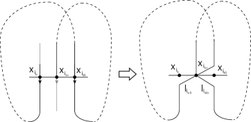
Figure 8. Deformation of orbit arcs in the case $x_{i_{k_{-}}}<x_{i_{k_{+}}}<x_{i_{k_{0}}}<x_{i}$

Note that if $S$ is orientable then we can choose $T_{i_{k_{-0}}}$ and $T_{i_{k_{0+}}}$ as closed transversals. This implies that $O^{+}(x_{i_{k+1_{-}}})\cap(T_{i_{k_{-0}}}\cup T_{i_{k_{0+}}})=\emptyset$. Hence $(T_{i_{k_{-0}}}\cup T_{i_{k_{0+}}})\cap(T_{i_{l_{-0}}}\cup T_{i_{l_{0+}}})=\emptyset$ for any $k\neq l$. Since these simple closed curves intersect exactly one point, they are essential. Cutting $T_{i_{1_{0+}}}$ and collapsing new boundary components into singletons, we obtain the resulting surface whose genus is the genus of $S$ minus one. Since there are infinitely many disjoint bouquets $T_{i_{k_{-0}}}\cup T_{i_{k_{0+}}}$, the genus of $S$ is not finite, which contradicts the compactness of $S$. Thus there is a large number $N>0$ such that $x_{i}<x_{i+1}$ in $I$ for any natural number $i\geq N$. By renumbering, the claim holds.

Denote by $I_{i}$ by the sub-arc of $I$ whose boundary consists of $x_{i}$ and $x_{i+1}$, and by $C_{i}$ the curve contained in $O^{+}(x_{0})$ whose boundary consists of $x_{i}$ and $x_{i+1}$. Let $D_{i}$ be the open subset bounded by the union $I_{i}\cup C_{i}\cup I_{i+1}\cup C_{i+1}$. Since there are at most finitely many genus, by renumbering $x_{i}$, we may assume that $D_{i}$ is a rectangle and so a flow box as in Figure 9 for any $i\in\mathbb{Z}_{\geq 0}$.

Figure 9. $D_{i}$ is the rectangle with $\partial D_{i}=I_{i}\cup C_{i}\cup I_{i+1}\cup C_{i+1}$ and $T_{i}$ is a closed transversal obtained by the waterfall construction to the loop $\partial D_{i}$.

By the waterfall construction to the loop $I_{i}\cup C_{i}$, we obtain a closed transversal $T_{i}$ near the loop $I_{i}\cup C_{i}$. Define a union $\mathbb{A}_{k}:=(\bigcup_{i=k}^{\infty}(D_{i}\cup I_{i+1}\cup C_{i+1}))-\{x_{k+1}\}$ for any $k\in\mathbb{Z}_{\geq 0}$. From the monotonicity of $x_{i}$ in $I$, renumbering $\mathbb{A}_{k}$, we may assume that each $\mathbb{A}_{k}$ is an open annulus homotopic to $\mathbb{A}_{0}$. By construction of the annulus $\mathbb{A}_{0}$, any positive orbit in $\mathbb{A}_{0}$ intersects with $T_{i}$ at most one time for any $i$. This implies that $\mathbb{A}_{0}\subseteq\mathrm{int}\mathrm{P}(v)$. Since $\omega(x_{0})$ is connected, by construction, the closure of any rectangle $D_{i}$ does not intersect $\omega(x_{0})$ and so $\mathbb{A}_{k}\cap\omega(x_{0})=\emptyset$. Therefore $\omega(x_{0})=\bigcap_{n\in\mathbb{R}_{\geq 0}}\overline{\{v_{t}(x_{0})\mid t>n\}}=\bigcap_{k\in\mathbb{Z}_{\geq 0}}\overline{\{v_{t}(x_{0})\mid t>k\}}=\bigcap_{i\geq 0}\overline{\mathbb{A}_{i}}=\partial\overline{\mathbb{A}_{0}}-(I_{0}\cup C_{0})$. This means that $\gamma$ is a boundary component of its semi-attracting collar basin $\mathbb{A}_{0}$. In particular, $x_{0}\in\mathrm{Sat}_{v}(\mathbb{A}_{0})\subseteq\mathrm{int}\mathrm{P}(v)$. ∎

Note that each collar basin does not intersect $\overline{\mathrm{LD}(v)\sqcup\mathrm{E}(v)}$.

Lemma 4.2.

An orbit contained in $\mathrm{P}(v)\cap\overline{\mathrm{LD}(v)\sqcup\mathrm{E}(v)}$ is a connecting separatrix.

Proof.

Fix a point $x\in\mathrm{P}(v)\cap\overline{\mathrm{LD}(v)\sqcup\mathrm{E}(v)}$. Theorem VI [6] implies that the orbit class $\hat{O}$ of an orbit $O\subseteq\mathrm{LD}(v)\sqcup\mathrm{E}(v)$ contains infinitely many strongly recurrent orbits and so we may assume that $x\in\omega(O)\cap\alpha(O)$. By the generalization of the Poincaré-Bendixson theorem for a flow with finitely many singular points (cf. Theorem 2.6.1 [29]), the $\omega$-limit set of $x$ is either a singular point, a semi-attracting limit circuit, or a Q-set. Assume that the $\omega$-limit set $\omega(x)$ is a semi-attracting limit circuit. Then $x\in\mathrm{int}\mathrm{P}(v)$ and so $O\cap\mathrm{P}(v)\neq\emptyset$, which contradicts $O\subseteq\mathrm{LD}(v)\sqcup\mathrm{E}(v)$. Assume that $\omega(x)$ is a Q-set. Since $x$ is not recurrent, we have $\omega(x)\neq\overline{O}$. Since $\omega(x)\subseteq\overline{O}$, Proposition 2.2 [47] implies that $\omega(x)=\overline{O}$, which contradicts $\omega(x)\neq\overline{O}$. Thus the $\omega$-limit set $\omega(x)$ is a singular point. By symmetry, the $\alpha$-limit set $\alpha(x)$ is a singular point. ∎

In general, the union $\mathrm{LD}(v)$ of a flow is not open even if singular points are countable. In fact, there is a toral flow with $\partial\mathrm{LD}(v)=\partial\mathrm{P}(v)=\mathbb{T}^{2}$ (cf. Example 2.10 [47]) such that isolated singular points converge to a singular point. On the other hand, the finiteness implies the following properties.

Lemma 4.3.

We have $\mathrm{LD}(v)\cap\overline{\mathrm{P}(v)}=\emptyset$.

Proof.

By Lemma 3.1, we may assume that $S$ is connected and orientable. Assume that there is a point $x\in\mathrm{LD}(v)\cap\overline{\mathrm{P}(v)}$. Theorem VI [6] implies that the orbit class $\hat{O}(x)$ contains infinitely many strongly recurrent orbits and so there is a non-closed recurrent point $z$ with $x\in\omega(z)\cap\alpha(z)$. Since the orbit closure $\overline{O(x)}$ is a neighborhood of $x$, there is a sequence $(x_{n})_{n\in\mathbb{Z}_{>0}}$ in $\overline{O(x)}\cap\partial^{-}\mathrm{P}(v)\subseteq\overline{\mathrm{LD}(v)}$ converging to $x$ such that $O(x_{n})\cap O(x_{m})=\emptyset$ for any $n\neq m\in\mathbb{Z}_{>0}$. Then $x_{n}\in\omega(z)\cap\alpha(z)$ for any $n\in\mathbb{Z}_{>0}$. Since neither $\omega(x_{n})$ nor $\alpha(x_{n})$ are limit cycles, Lemma 3.7 and the dual statement for $\alpha$-limit sets imply that $\overline{O(x_{n})}-O(x_{n})$ consists of at most two singular points. Fix an open flow box $U\subset\overline{O(x)}$ centered at $x$. By renumbering, we may assume that $(x_{n})_{n\in\mathbb{Z}_{>0}}$ converges to $x$ decreasing with respect to the transverse direction from one side in the flow box.

We claim that there is a subsequence $(x_{k_{n}})_{n\in\mathbb{Z}_{>0}}$ of $(x_{n})_{n\in\mathbb{Z}_{>0}}$ such that $\overline{O(x_{n})}$ is a simple closed curve. Indeed, suppose that there is no subsequence $(x_{k_{n}})_{n\in\mathbb{Z}_{>0}}$ of $(x_{n})_{n\in\mathbb{Z}_{>0}}$ such that $\overline{O(x_{n})}$ is a simple closed curve. By renumbering, each closure $\overline{O(x_{n})}$ is not a simple closed curve. Then $\omega(x_{n})\neq\alpha(x_{n})$ for any $n\in\mathbb{Z}_{>0}$. Since $|\mathop{\mathrm{Sing}}(v)|<\infty$, there are singular points $\alpha\neq\omega\in\overline{\mathrm{LD}(v)}$ and a subsequence $(x_{k_{n}})_{n\in\mathbb{Z}_{>0}}$ of $(x_{n})_{n\in\mathbb{Z}_{>0}}$ such that $\omega(x_{k_{n}})=\omega$ and $\alpha(x_{k_{n}})=\alpha$. Since $S$ is compact, there are an open disk $D\subseteq\overline{O(x)}$ and three points $x_{n_{1}},x_{n_{2}},x_{n_{3}}$ in the subsequence such that $\partial D=\overline{O(x_{n_{1}})}\cup\overline{O(x_{n_{3}})}$ and $x_{n_{2}}\in\mathrm{int}D$. Then $\overline{\mathrm{LD}(v)}\cap\mathrm{int}D=\emptyset$ and so $x_{n_{2}}\notin\overline{\mathrm{LD}(v)}$, which contradicts the choice of $x_{n_{2}}$.

By renumbering, we may assume that there is a singular point $\gamma$ with $\omega(x_{n})=\alpha(x_{n})=\gamma$ for any $n\in\mathbb{Z}_{>0}$. Since there are at most finitely many isotopic classes of loops, we may assume that any pair of $\overline{O(x_{n})}$ and $\overline{O(x_{m})}$ are homotopic relative to $\gamma$. If $\overline{O(x_{n})}$ is essential or parallel to $\partial S$, then a connected component of $\overline{O(x_{n})}\cup\overline{O(x_{n+2})}$ containing $\overline{O(x_{n+1})}$ is an open disk, which contradicts $x_{n+1}\in\overline{O(X)}\subseteq\overline{\mathrm{LD}(v)}$. Thus $\overline{O(x_{n})}$ is null homotopic and so intersects no closed transversals. If $O(x_{n})\cap U$ consists of at least two maximal orbit arcs, then the waterfall construction to the loop consisting an orbit arc in $O(x_{n})$ and a transverse arc in $U$ implies the existence of a closed transversal intersecting $O(x_{n})$, which contradicts the non-existence of closed transversals. Therefore $O(x_{n})\cap U$ is one orbit arc. Since the complement $S-\overline{O(x_{n})}$ consists of two connected components and one of them is an open disk and since the sequence $(x_{n})_{n\in\mathbb{Z}_{>0}}$ converges to $x$ decreasing with respect to the transverse direction from one side in the flow box, the loop $O(x_{n+1})\sqcup\{\gamma\}=\overline{O(x_{n+1})}$ for any $n\in\mathbb{Z}_{>0}$ contains a disk which contains either $O(x_{n})$ or $O(x_{n+2})$, which contradicts $x_{n},x_{n+2}\in\overline{O(X)}\subseteq\overline{\mathrm{LD}(v)}$. Thus $\mathrm{LD}(v)\cap\overline{\mathrm{P}(v)}=\emptyset$. ∎

Lemma 4.4.

The union $\mathrm{LD}(v)$ is open.

Proof.

Since the singular point set $\mathop{\mathrm{Sing}}(v)$ is closed, Lemma 3.2 and Lemma 4.3 imply that $\overline{\mathop{\mathrm{Sing}}(v)\sqcup\mathop{\mathrm{Per}}(v)\sqcup\mathrm{P}(v)\sqcup\mathrm{E}(v)}\cap\mathrm{LD}(v)=\emptyset$ and so that the union $\mathrm{LD}(v)=S-\overline{\mathop{\mathrm{Sing}}(v)\sqcup\mathop{\mathrm{Per}}(v)\sqcup\mathrm{P}(v)\sqcup\mathrm{E}(v)}$ is open. ∎

We describe the border $\partial^{-}\mathrm{P}(v)=\mathrm{P}(v)-\mathrm{int}\mathrm{P}(v)$ as follows.

Proposition 4.5.

Let $v$ be a flow with finitely many singular points on a compact surface. Then each orbit in $\partial^{-}\mathrm{P}(v)$ is a connecting separatrix. Moreover, if $v$ is quasi-regular, then $\partial^{-}\mathrm{P}(v)$ is a finite union of multi-saddle separatrices.

Proof.

Fix an orbit $O$ in $\partial^{-}\mathrm{P}(v)$. By Lemma 3.3, we have $\overline{O}\cap\mathop{\mathrm{Per}}(v)=\emptyset$. Since $\partial^{-}\mathrm{P}(v)=\mathrm{P}(v)-\mathrm{int}\mathrm{P}(v)=\mathrm{P}(v)\cap\overline{\mathop{\mathrm{Sing}}(v)\sqcup\mathop{\mathrm{Per}}(v)\sqcup\mathrm{LD}(v)\sqcup\mathrm{E}(v)}=\mathrm{P}(v)\cap\overline{\mathop{\mathrm{Per}}(v)\sqcup\mathrm{LD}(v)\sqcup\mathrm{E}(v)}$, we have $O\subseteq\mathrm{P}(v)\cap\overline{\mathop{\mathrm{Per}}(v)\sqcup\mathrm{LD}(v)\sqcup\mathrm{E}(v)}$. By Lemma 4.2, we may assume that $O\subseteq\mathrm{P}(v)\cap\overline{\mathop{\mathrm{Per}}(v)}$. Lemma 3.2 implies that $\overline{O}\subseteq\overline{\mathop{\mathrm{Per}}(v)}-\mathop{\mathrm{Per}}(v)=\partial^{+}\mathop{\mathrm{Per}}(v)\subseteq\partial^{-}\mathop{\mathrm{Sing}}(v)\sqcup\partial^{-}\mathrm{P}(v)$. By the generalization of the Poincaré-Bendixson theorem for a flow with finitely many singular points, the $\omega$-limit (resp. $\alpha$-limit) set of $O$ is either a singular point, or a semi-attracting (resp. semi-repelling) limit circuit. Since $O\subseteq\partial^{-}\mathrm{P}(v)$, by Lemma 4.1, the $\omega$-limit and $\alpha$-limit sets of $O$ contain no limit circuits and so each of them is a singular point. Therefore $O$ is a connecting separatrix.

Suppose that $v$ is quasi-regular. Since any points whose $\omega$-limit set is either a $\partial$-sink, a sink, or a semi-attracting limit circuit is contained in $\mathrm{int}\mathrm{P}(v)$, the $\omega$-limit set $\omega(O)$ is neither $\partial$-sink, a sink, nor a semi-attracting limit circuit. This means that the $\omega$-limit set $\omega(O)$ is a multi-saddle. By symmetry, so is $\alpha$-limit set $\alpha(O)$. ∎

The finiteness of $\mathop{\mathrm{Sing}}(v)$ is necessary. In fact, there is a flow with a point $y\in\partial^{-}\mathrm{P}(v)$ whose $\omega$-limit set is not a point (see Figure 10).

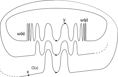
Figure 10. An $\omega$-limit set which is not arcwise-connected.

The quasi-regularity of $\mathop{\mathrm{Sing}}(v)$ is necessary. In fact, there is a flow with infinitely many connecting separatrices (see Figure 6). Notice that the union $\mathop{\mathrm{P}_{\mathrm{semi}}}(v)$ is the union of semi-multi-saddle separatrices if $v$ is quasi-regular, because any weak saddles for a quasi-regular flow are multi-saddles. The previous proposition and Lemma 2.1 implies the following statement.

Corollary 4.6.

If $v$ is quasi-regular, then the union $\partial^{-}\mathrm{P}(v)\sqcup\mathop{\mathrm{P}_{\mathrm{ms}}}(v)\sqcup\mathop{\mathrm{P}_{\mathrm{ss}}}(v)$ is the union $\mathop{\mathrm{P}_{\mathrm{semi}}}(v)$ of semi-multi-saddle separatrices.

We obtain the following description of a neighborhood of $\mathrm{E}(v)$.

Lemma 4.7.

$\partial^{-}\mathrm{E}(v)=\mathrm{E}(v)\subseteq\mathrm{int}(\mathrm{E}(v)\sqcup\mathrm{int}\mathrm{P}(v))=\mathrm{E}(v)\sqcup\mathrm{int}\mathrm{P}(v)$.

Proof.

By the Maǐer theorem, the closure $\overline{\mathrm{E}(v)}$ is the finite union of closures of exceptional orbits and so $\partial^{-}\mathrm{E}(v)=\mathrm{E}(v)$. The closedness of $\mathop{\mathrm{Sing}}(v)$ and Lemma 3.2 imply $\mathrm{E}(v)\cap\overline{\mathop{\mathrm{Sing}}(v)\sqcup\mathop{\mathrm{Per}}(v)\sqcup\mathrm{LD}(v)}=\emptyset$. Then we have that $\mathrm{E}(v)\subseteq S-\overline{\mathop{\mathrm{Sing}}(v)\sqcup\mathop{\mathrm{Per}}(v)\sqcup\mathrm{LD}(v)}=\mathrm{int}(\mathrm{P}(v)\sqcup\mathrm{E}(v))$.

We claim that $\overline{\partial^{-}\mathrm{P}(v)}\cap\mathrm{E}(v)=\emptyset$. Indeed, assume there is a point $x\in\overline{\partial^{-}\mathrm{P}(v)}\cap\mathrm{E}(v)$. Then there are a sequence $\{O_{n}\}_{n\in\mathbb{Z}_{>0}}$ of orbits in $\partial^{-}\mathrm{P}(v)$ and a transverse closed arc $\gamma$ with $x\in\partial\gamma\setminus\bigcup_{n}O_{n}$ such that $x\in\overline{\bigcup_{n}O_{n}\cap\gamma}$ and $O_{n}\neq O_{m}$ for any $n\neq m$. Suppose that there are infinitely many orbits $O_{k_{n}}$ which are homoclinic. Taking a subsequence, we may assume that there is a singular point $y$ with $y=\omega(O_{n})=\alpha(O_{n})$ for any $n$. Since $S$ is compact, taking a subsequence, we may assume that $\{y\}\sqcup O_{n}$ and $\{y\}\sqcup O_{n+1}$ are homotopic relative to $\{y\}$. As above, taking a subsequence, we may assume that a union $\{y\}\sqcup O_{2n}\sqcup O_{2n+2}$ bounds an open disk $B_{n}$ for any $n$. Then $B_{n}$ is an open disk which contains $O_{2n+1}$ such that $B_{n}-O_{2n+1}$ consists of two open disks. By $O_{2n+1}\subset\partial^{-}\mathrm{P}(v)$, let $C_{n}$ be the one of two open disks $B_{n}-O_{2n+1}$ intersecting $S-\mathrm{P}(v)$. Since an open disk whose boundary is saturated does not intersect $\mathrm{LD}(v)\sqcup\mathrm{E}(v)$, the disk $C_{n}$ intersects $S-(\mathrm{P}(v)\sqcup\mathrm{LD}(v)\sqcup\mathrm{E}(v))=\mathop{\mathrm{Sing}}(v)\sqcup\mathop{\mathrm{Per}}(v)$. Since a null homotopic periodic orbit bounds a singular point, the disk $C_{n}$ contains singular points. Hence there are infinitely many singular points, which contradicts the finite hypothesis of singular points. Thus there are at most finitely many orbits $O_{k_{n}}$ which are homoclinic. Taking a subsequence, we may assume that there are singular points $\alpha\neq\omega$ with $\omega=\omega(O_{n})$ and $\alpha=\alpha(O_{n})$ for any $n$. Since $S$ is compact, taking a subsequence, we may assume that $\{y\}\sqcup O_{n}$ and $\{y\}\sqcup O_{n+1}$ are homotopic relative to $\{\alpha,\omega\}$. As above, taking a subsequence, we may assume that a union $\{\alpha,\omega\}\sqcup O_{2n}\sqcup O_{2n+2}$ bounds an open disk $B_{n}$ for any $n$. Then $B_{n}$ is an open disk which contains $O_{2n+1}$ such that $B_{n}-O_{2n+1}$ consists of two open disks. By $O_{2n+1}\subset\partial^{-}\mathrm{P}(v)$, let $C_{n}$ be the one of two open disks $B_{n}-O_{2n+1}$ intersecting $S-\mathrm{P}(v)$. Since $\partial C_{n}\subset\{\alpha,\omega\}\sqcup O_{2n}\sqcup\sqcup O_{2n+1}\sqcup O_{2n+2}$, the disk $C_{n}$ intersects $S-(\mathrm{P}(v)\sqcup\mathrm{LD}(v)\sqcup\mathrm{E}(v))=\mathop{\mathrm{Sing}}(v)\sqcup\mathop{\mathrm{Per}}(v)$. Since a null homotopic periodic orbit bounds a singular point, the disk $C_{n}$ contains singular points. Hence there are infinitely many singular points, which contradicts the finite hypothesis of singular points. This completes the claim.

Then $\mathrm{int}(\mathrm{E}(v)\sqcup\mathrm{P}(v))\setminus\overline{\partial^{-}\mathrm{P}(v)}\subseteq(\mathrm{E}(v)\sqcup\mathrm{P}(v))\setminus\overline{\partial^{-}\mathrm{P}(v)}=\mathrm{E}(v)\sqcup\mathrm{int}\mathrm{P}(v)$ is an open neighborhood of $\mathrm{E}(v)$. Since $\mathrm{int}\mathrm{P}(v)\subset\mathrm{int}(\mathrm{E}(v)\sqcup\mathrm{P}(v))$, we have $E\sqcup\mathrm{int}\mathrm{P}(v)\subseteq\mathrm{int}(\mathrm{E}(v)\sqcup\mathrm{int}\mathrm{P}(v))$ and so $\mathrm{int}(\mathrm{E}(v)\sqcup\mathrm{int}\mathrm{P}(v))=\mathrm{E}(v)\sqcup\mathrm{int}\mathrm{P}(v)$. ∎

Recall the coborder $\partial^{+}A=\overline{A}-A$ of a subset $A\subseteq S$. The following coborder’s property holds.

Lemma 4.8.

$\mathrm{E}(v)\subseteq\partial^{+}\mathrm{P}(v)\subseteq\mathop{\mathrm{Sing}}(v)\sqcup\partial^{-}\mathop{\mathrm{Per}}(v)\sqcup\mathrm{E}(v)$.

Proof.

By Lemma 2.3 [47], we obtain $\mathrm{E}(v)\subseteq\overline{\mathrm{int}\mathrm{P}(v)}\setminus\mathrm{P}(v)\subseteq\partial^{+}\mathrm{P}(v)$. Since the union $\mathrm{LD}(v)\sqcup\mathrm{int}\mathop{\mathrm{Per}}(v)$ are open, we have $\overline{\mathrm{P}(v)}-(\mathrm{P}(v)\sqcup\mathrm{E}(v))\subseteq S-(\mathrm{int}\mathop{\mathrm{Per}}(v)\sqcup\mathrm{P}(v)\sqcup\mathrm{LD}(v)\sqcup\mathrm{E}(v))=\mathop{\mathrm{Sing}}(v)\sqcup\partial^{-}\mathop{\mathrm{Per}}(v)$. ∎

4.2. Boundaries, borders, and coborders

We summarize the properties of the boundary points and those of (co)border points as follows.

Proposition 4.9.

Let $v$ be a flow with finitely many singular points on a compact surface $S$. The following statements hold:
$(1)$ $\partial^{+}\mathrm{LD}(v)=\partial\mathrm{LD}(v)$ $(\mathrm{i.e.}\,\,\mathrm{LD}(v)$ is open $)$.
$(2)$ $\partial^{+}\mathop{\mathrm{Sing}}(v)=\emptyset$.
$(3)$ $\partial^{+}\mathop{\mathrm{Per}}(v)\sqcup\partial^{+}\mathrm{LD}(v)\sqcup\partial^{+}\mathrm{E}(v)\subseteq\mathop{\mathrm{Sing}}(v)\sqcup\partial^{-}\mathrm{P}(v)$.
$(4)$ $\partial^{+}\mathrm{P}(v)\subseteq\mathop{\mathrm{Sing}}(v)\sqcup\partial^{-}\mathop{\mathrm{Per}}(v)\sqcup\mathrm{E}(v)$.

Proof.

The assertion $(1)$ is immediate from Lemma 4.4. The finiteness of $\mathop{\mathrm{Sing}}(v)$ implies the assertion $(2)$. The assertion $(3)$ is obtained by Lemma 3.2. The assertion $(4)$ is assured by Lemma 4.8. ∎

Proposition 4.10.

Let $v$ be a flow with finitely many singular points on a compact surface $S$. The following statements hold:
$(1)$ $\partial^{-}\mathop{\mathrm{Sing}}(v)=\mathop{\mathrm{Sing}}(v)$.
$(2)$ $\partial^{-}\mathop{\mathrm{Per}}(v)\subseteq\overline{\mathrm{int}\mathrm{P}(v)}$ is contained in the closure of the union of limit cycles.
$(3)$ $\partial^{-}\mathrm{P}(v)=(\partial^{+}\mathop{\mathrm{Per}}(v)\cup\partial^{+}\mathrm{LD}(v)\cup\partial^{+}\mathrm{E}(v))\setminus\mathop{\mathrm{Sing}}(v)$ consists of connecting separatrices.
$(4)$ $\partial^{-}\mathrm{LD}(v)=\emptyset$.
$(5)$ $\partial^{-}\mathrm{E}(v)=\mathrm{E}(v)=\partial^{+}\mathrm{P}(v)\cap\mathrm{int}(\mathrm{E}(v)\sqcup\mathrm{int}\mathrm{P}(v))$.

Moverover, a disjoint union $\mathop{\mathrm{Sing}}(v)\sqcup\partial^{-}\mathop{\mathrm{Per}}(v)\sqcup\partial^{-}\mathrm{P}(v)\sqcup\mathrm{E}(v)$ is closed.

Proof.

The finiteness of $\mathop{\mathrm{Sing}}(v)$ implies the assertion $(1)$. The assertion $(2)$ is followed by Lemma 3.4. Proposition 4.5 and Proposition 4.9 imply the assertion $(3)$. The assertion $(4)$ is obtained by Lemma 4.4. From Lemma 4.7, the assertion $(5)$ holds. ∎

Proposition 4.11.

Let $v$ be a flow with finitely many singular points on a compact surface $S$. The following statements hold:
$(1)$ $\partial\mathop{\mathrm{Per}}(v)\subseteq\mathop{\mathrm{Sing}}(v)\sqcup\partial^{-}\mathop{\mathrm{Per}}(v)\sqcup\partial^{-}\mathrm{P}(v)$.
$(2)$ $\partial\mathrm{LD}(v)=\partial^{+}\mathrm{LD}(v)\subseteq\mathop{\mathrm{Sing}}(v)\sqcup\partial^{-}\mathrm{P}(v)$.
$(3)$ $\partial\mathrm{E}(v)=\overline{E}\subseteq\mathop{\mathrm{Sing}}(v)\sqcup\partial^{-}\mathrm{P}(v)\sqcup\mathrm{E}(v)$.
$(4)$ $\partial\mathrm{P}(v)\subseteq\mathop{\mathrm{Sing}}(v)\sqcup\partial^{-}\mathop{\mathrm{Per}}(v)\sqcup\partial^{-}\mathrm{P}(v)\sqcup\mathrm{E}(v)$.
$(5)$ $\partial^{-}\mathrm{P}(v)$ is a union of connecting separatrices.
$(6)$ $\partial^{-}\mathop{\mathrm{Per}}(v)$ is contained in the closure of the union of limit cycles.

Proof.

Proposition 4.9 implies the assertions (1) - (4). Proposition 4.5 implies the assertion (5). Lemma 3.4 implies the assertion (6). ∎

4.3. Descriptions of border point sets and relative concepts

Finiteness of singular points is necessary in the previous proposition (3). In fact, a construction in Figure 10 implies that there is a flow with an orbit in $\partial^{-}\mathrm{P}(v)\cap(\partial^{+}\mathrm{LD}(v)\cup\partial^{+}\mathrm{E}(v))$ which is not a separatrix. Recall that $\mathop{\mathrm{BD}}(v)=\mathop{\mathrm{Bd}}(v)\sqcup\mathop{\mathrm{Per}}_{1}(v)$ and $\mathop{\mathrm{Bd}}(v)=\partial\mathop{\mathrm{Sing}}(v)\cup\partial\mathop{\mathrm{Per}}(v)\cup\partial_{\mathop{\mathrm{Per}}(v)}\cup\partial\mathrm{P}(v)\cup\partial\mathrm{LD}(v)\cup\mathop{\mathrm{P}_{\mathrm{sep}}}(v)\cup\partial\mathrm{E}(v)$. Describe the (strict) border point set as follows.

Lemma 4.12.

The following statements holds for a flow $v$ with finitely many singular points on a compact surface $S$:
(1) $\mathop{\mathrm{Bd}}(v)$ and $\mathop{\mathrm{BD}}(v)$ are closed.
(2) $\mathop{\mathrm{BD}}(v)=\mathop{\mathrm{Sing}}(v)\sqcup\partial^{-}\mathop{\mathrm{Per}}(v)\sqcup\partial_{\mathop{\mathrm{Per}}(v)}\sqcup\mathop{\mathrm{Per}}_{1}(v)\sqcup\partial^{-}\mathrm{P}(v)\sqcup\mathop{\mathrm{P}_{\mathrm{sep}}}(v)\sqcup\mathrm{E}(v)$.
(3) The union $\mathop{\mathrm{P}_{\mathrm{ms}}}(v)\sqcup\mathop{\mathrm{P}_{\mathrm{ss}}}(v)\sqcup\mathop{\partial_{\mathrm{P}(v)}}$ consists of finitely many connecting separatrices.
(4) The union $\partial_{\mathop{\mathrm{Per}}(v)}\sqcup\mathop{\mathrm{Per}}_{1}(v)$ is the finite union of one-sided periodic orbits in $\mathrm{int}\mathop{\mathrm{Per}}(v)$.
(5) If there are at most finitely many limit cycles, then the union $\partial^{-}\mathop{\mathrm{Per}}(v)$ is the finite union of limit cycles.
(6) If $v$ is quasi-regular, then the union $\partial^{-}\mathrm{P}(v)\sqcup\mathop{\mathrm{P}_{\mathrm{sep}}}(v)=\mathop{\mathrm{P}_{\mathrm{semi}}}(v)\sqcup\mathop{\partial_{\mathrm{P}(v)}}$ is the finite union of semi-multi-saddle separatrices and separatrices on $\partial S$ between $\partial$-sources and $\partial$-sinks. In particular, the quasi-regularity implies $\partial^{-}\mathrm{P}(v)\subseteq\mathop{\mathrm{P}_{\mathrm{semi}}}(v)$.

Proof.

By definitions, the assertion (4) holds. From Proposition 4.10, the assertion (5) holds. The compactness of $S$ implies that there are at most finitely connected components of $\partial S$ and so that $\mathop{\mathrm{Per}}_{1}(v)$ consists of finitely many orbits. Therefore $\mathop{\mathrm{Bd}}(v)$ is closed if and only if so is $\mathop{\mathrm{BD}}(v)$. The finite union $\partial\mathop{\mathrm{Sing}}(v)\cup\partial\mathop{\mathrm{Per}}(v)\cup\partial\mathrm{P}(v)\cup\partial\mathrm{LD}(v)\cup\partial\mathrm{E}(v)\cup\partial_{\mathop{\mathrm{Per}}(v)}$ of boundaries is closed. By the finite existence of multi-saddles, the union of semi-multi-saddle separatrices consists of finitely many orbits and so does the union $\mathop{\mathrm{P}_{\mathrm{ms}}}(v)\sqcup\mathop{\mathrm{P}_{\mathrm{ss}}}(v)$ of semi-multi-saddle separatrices in $\mathrm{int}\mathrm{P}(v)$. The compactness of $S$ implies that there are at most finitely connected components of $\partial S$ and so that $\mathop{\partial_{\mathrm{P}(v)}}$ consists of finitely many orbits. By definition of $\mathop{\mathrm{P}_{\mathrm{sep}}}(v)=(\mathop{\mathrm{P}_{\mathrm{lc}}}(v)\cup\mathop{\mathrm{P}_{\mathrm{ms}}}(v))\sqcup\mathop{\mathrm{P}_{\mathrm{ss}}}(v)\sqcup\mathop{\partial_{\mathrm{P}(v)}}$, the assertion (3) holds. Moreover, the closure of the finite union $\mathop{\mathrm{P}_{\mathrm{sep}}}(v)$ of orbits is the finite union of the closures of orbits in $\mathop{\mathrm{P}_{\mathrm{sep}}}(v)$. Therefore $\overline{\mathop{\mathrm{P}_{\mathrm{sep}}}(v)}\subseteq\mathop{\mathrm{Sing}}(v)\sqcup\mathop{\mathrm{P}_{\mathrm{sep}}}(v)$. This implies that $\mathop{\mathrm{Bd}}(v)$ is closed and so is $\mathop{\mathrm{BD}}(v)$. Thus the assertion (1) holds.

The finiteness of $\mathop{\mathrm{Sing}}(v)$ implies $\partial\mathop{\mathrm{Sing}}(v)=\mathop{\mathrm{Sing}}(v)$. Proposition 4.9 and Proposition 4.10 imply that $\partial\mathrm{LD}(v)\subseteq\mathop{\mathrm{Sing}}(v)\sqcup\partial^{-}\mathrm{P}(v)$ and that $\partial\mathrm{E}(v)=\overline{\mathrm{E}(v)}\subseteq\mathop{\mathrm{Sing}}(v)\cup\partial^{-}\mathrm{P}(v)\sqcup\mathrm{E}(v)$. Lemma 3.2 implies $\partial\mathop{\mathrm{Per}}(v)\subseteq\mathop{\mathrm{Sing}}(v)\sqcup\partial^{-}\mathop{\mathrm{Per}}(v)\sqcup\partial^{-}\mathrm{P}(v)$, and Lemma 4.8 implies $\partial\mathrm{P}(v)\subseteq\partial^{-}\mathrm{P}(v)\sqcup\mathrm{E}(v)\sqcup\mathop{\mathrm{Sing}}(v)\sqcup\partial^{-}\mathop{\mathrm{Per}}(v)$. Therefore $\mathop{\mathrm{Bd}}(v)=\partial\mathop{\mathrm{Sing}}(v)\cup\partial\mathop{\mathrm{Per}}(v)\cup\partial_{\mathop{\mathrm{Per}}(v)}\cup\partial\mathrm{P}(v)\cup\mathop{\mathrm{P}_{\mathrm{sep}}}(v)\cup\partial\mathrm{LD}(v)\cup\partial\mathrm{E}(v)=\mathop{\mathrm{Sing}}(v)\sqcup\partial^{-}\mathop{\mathrm{Per}}(v)\sqcup\partial_{\mathop{\mathrm{Per}}(v)}\sqcup\partial^{-}\mathrm{P}(v)\sqcup\mathop{\mathrm{P}_{\mathrm{sep}}}(v)\sqcup\mathrm{E}(v)$. This completes the assertion (2).

Suppose that $v$ is quasi-regular. From Corollary 4.6, the union $\partial^{-}\mathrm{P}(v)\sqcup\mathop{\mathrm{P}_{\mathrm{ms}}}(v)\sqcup\mathop{\mathrm{P}_{\mathrm{ss}}}(v)$ is the finite union of semi-multi-saddle separatrices. The quasi-regularity implies $\mathop{\mathrm{P}_{\mathrm{sep}}}(v)=\mathop{\mathrm{P}_{\mathrm{ms}}}(v)\sqcup\mathop{\mathrm{P}_{\mathrm{ss}}}(v)\sqcup\mathop{\partial_{\mathrm{P}(v)}}$. Therefore the union $\partial^{-}\mathrm{P}(v)\sqcup\mathop{\mathrm{P}_{\mathrm{sep}}}(v)$ is the finite union of semi-multi-saddle separatrices and separatrices on $\partial S$ between $\partial$-sources and $\partial$-sinks. ∎

4.4. Complement of the strict border point set

We have the following properties.

Proposition 4.13.

The following statements hold for a flow $v$ with finitely many on a compact surface $S$:
$(1)$ The complement $S-\mathop{\mathrm{Bd}}(v)$ is open.
$(2)$ $S-\mathop{\mathrm{Bd}}(v)=(\mathrm{int}\mathop{\mathrm{Per}}(v)-\partial_{\mathop{\mathrm{Per}}(v)})\sqcup(\mathrm{int}\mathrm{P}(v)-\mathop{\mathrm{P}_{\mathrm{sep}}}(v))\sqcup\mathrm{LD}(v)$.
$(3)$ The invariant subsets $\mathrm{int}\mathop{\mathrm{Per}}(v)-\partial_{\mathop{\mathrm{Per}}(v)}$, $\mathrm{int}\mathrm{P}(v)-\mathop{\mathrm{P}_{\mathrm{sep}}}(v)$, and $\mathrm{LD}(v)$ are open.
$(4)$ The union $\mathrm{LD}(v)/\hat{v}$ is a finite space.
$(5)$ If $v$ is quasi-regular, then the set differences $\mathrm{P}(v)-\mathop{\mathrm{P}_{\mathrm{semi}}}(v)$ and $\mathrm{P}(v)-(\mathop{\mathrm{P}_{\mathrm{semi}}}(v)\sqcup\mathop{\partial_{\mathrm{P}(v)}})=\mathrm{int}\mathrm{P}(v)-\mathop{\mathrm{P}_{\mathrm{sep}}}(v)$ are open.

Proof.

Lemma 4.12 implies the assertion (1). By $\mathop{\mathrm{Bd}}(v)=\mathop{\mathrm{Sing}}(v)\sqcup\partial^{-}\mathop{\mathrm{Per}}(v)\sqcup\partial_{\mathop{\mathrm{Per}}(v)}\sqcup\partial^{-}\mathrm{P}(v)\sqcup\mathop{\mathrm{P}_{\mathrm{sep}}}(v)\sqcup\mathrm{E}(v)$, we have $S-\mathop{\mathrm{Bd}}(v)=(\mathrm{int}\mathop{\mathrm{Per}}(v)-\partial_{\mathop{\mathrm{Per}}(v)})\sqcup(\mathrm{int}\mathrm{P}(v)-\mathop{\mathrm{P}_{\mathrm{sep}}}(v))\sqcup\mathrm{LD}(v)$. This means that the assertion (2) holds. By the finiteness of the boundary components, the set difference $\mathrm{int}\mathop{\mathrm{Per}}(v)-\partial_{\mathop{\mathrm{Per}}(v)}$ is open. Since $\mathop{\mathrm{Bd}}(v)$ is closed, the set difference $\mathrm{int}\mathrm{P}(v)\setminus\mathop{\mathrm{Bd}}(v)=\mathrm{int}\mathrm{P}(v)\setminus(\mathop{\mathrm{Sing}}(v)\sqcup\partial^{-}\mathop{\mathrm{Per}}(v)\sqcup\partial_{\mathop{\mathrm{Per}}(v)}\sqcup\partial^{-}\mathrm{P}(v)\sqcup\mathop{\mathrm{P}_{\mathrm{sep}}}(v)\sqcup\mathrm{E}(v))=\mathrm{int}\mathrm{P}(v)-\mathop{\mathrm{P}_{\mathrm{sep}}}(v)$ is open. Lemma 4.4 implies the openness of the union $\mathrm{LD}(v)$. Thus the assertion $(3)$ is true. By Proposition 2.2 [47], the union $\mathrm{LD}(v)$ consists of finitely many orbit classes. The assertion $(4)$ is immediate from this finiteness.

Suppose that $v$ is quasi-regular. The set difference $\mathrm{P}(v)-(\mathop{\mathrm{P}_{\mathrm{semi}}}(v)\sqcup\mathop{\partial_{\mathrm{P}(v)}})=\mathrm{int}\mathrm{P}(v)-\mathop{\mathrm{P}_{\mathrm{sep}}}(v)$ is open. Since $\mathop{\partial_{\mathrm{P}(v)}}$ consists of finitely many orbits, the closure $\overline{\mathop{\mathrm{P}_{\mathrm{semi}}}(v)}\subseteq\mathop{\mathrm{Sing}}(v)\sqcup\mathop{\mathrm{P}_{\mathrm{semi}}}(v)$ is a union of $\mathop{\mathrm{P}_{\mathrm{semi}}}(v)$, $\partial$-sinks, and $\partial$-sources. Therefore the set difference $\mathrm{P}(v)-\mathop{\mathrm{P}_{\mathrm{semi}}}(v)=\mathrm{P}(v)\setminus\overline{\mathop{\mathrm{P}_{\mathrm{semi}}}(v)}$ is open. ∎

4.5. Border point sets for quasi-regular flows

The previous lemma and the following statement.

Proposition 4.14.

The following statements holds for a quasi-regular flow $v$ on a compact surface $S$:
(1) The border point set $\mathop{\mathrm{BD}}(v)$ is the union of singular points, one-sided periodic orbits, the closure of the union of limit cycles, semi-multi-saddle separatrices, separatrices between a $\partial$-source and a $\partial$-sink on the boundary $\partial S$, and exceptional orbits.
(2) The strict border point set $\mathop{\mathrm{Bd}}(v)$ is the union of singular points, periodic orbits on $\partial S$, the closure of the union of limit cycles, semi-multi-saddle separatrices, separatrices between a $\partial$-source and a $\partial$-sink on the boundary $\partial S$, and exceptional orbits.
(3) If there are at most finitely many limit cycles, then $\mathop{\mathrm{BD}}(v)\sqcup\mathrm{LD}(v)$ and $\mathop{\mathrm{Bd}}(v)\sqcup\mathrm{LD}(v)$ consist of finitely many orbit classes.
(4) If $v$ is of finite type, then $\mathop{\mathrm{BD}}(v)$ (resp. $\mathop{\mathrm{Bd}}(v)$) is the finite union of singular points, one-sided periodic orbits (resp. periodic orbits on $\partial S$), limit cycles, semi-multi-saddle separatrices, and separatrices between a $\partial$-source and a $\partial$-sink on the boundary $\partial S$.

Proof.

From Lemma 4.12, we have $\mathop{\mathrm{BD}}(v)=\mathop{\mathrm{Sing}}(v)\sqcup\partial^{-}\mathop{\mathrm{Per}}(v)\sqcup\partial_{\mathop{\mathrm{Per}}(v)}\sqcup\mathop{\mathrm{Per}}_{1}(v)\sqcup\mathop{\mathrm{P}_{\mathrm{semi}}}(v)\sqcup\mathop{\partial_{\mathrm{P}(v)}}\sqcup\mathrm{E}(v)$. Lemma 3.4 implies that $\partial^{-}\mathop{\mathrm{Per}}(v)$ is contained in the closure of the union of limit cycles. From Proposition 4.11, the closure of the union of limit cycles is contained in $\overline{\partial^{-}\mathop{\mathrm{Per}}(v)}\subseteq\partial\mathop{\mathrm{Per}}(v)\subseteq\mathop{\mathrm{Sing}}(v)\sqcup\partial^{-}\mathop{\mathrm{Per}}(v)\sqcup\partial^{-}\mathrm{P}(v)\subseteq\mathop{\mathrm{BD}}(v)$. Lemma 4.12 implies that $\partial_{\mathop{\mathrm{Per}}(v)}\sqcup\mathop{\mathrm{Per}}_{1}(v)$ is the finite union of one-sided periodic orbits in $\mathrm{int}\mathop{\mathrm{Per}}(v)$. The union of of one-sided periodic orbits is contained in $\partial^{-}\mathop{\mathrm{Per}}(v)\sqcup\partial_{\mathop{\mathrm{Per}}(v)}\sqcup\mathop{\mathrm{Per}}_{1}(v)\subseteq\mathop{\mathrm{BD}}(v)$. Therefore the assertion (1) holds. By definitions of (strict) border point set, the assertion (2) is followed from the assertion (1).

Suppose that there are at most finitely many limit cycles. By the finiteness of limit cycles, Lemma 3.4 implies that $\partial^{-}\mathop{\mathrm{Per}}(v)$ is the finite union of limit cycles. Compactness implies that $\partial_{\mathop{\mathrm{Per}}(v)}$ consists of finitely many orbits contained in the boundary $\partial S$ and so that the union $\partial_{\mathop{\mathrm{Per}}(v)}\sqcup\mathop{\mathrm{Per}}_{1}(v)$ of one-sided periodic orbits in $\mathrm{int}\mathop{\mathrm{Per}}(v)$ consists of finitely many orbits. Quasi-regularity implies that $\mathop{\mathrm{P}_{\mathrm{semi}}}(v)$ is the finite union of multi-saddle separatrices. By finiteness of $\mathop{\mathrm{Sing}}(v)$ and boundary components, the union $\mathop{\partial_{\mathrm{P}(v)}}$ is the finite union of separatrices between a $\partial$-source and a $\partial$-sink on the boundary $\partial S$. The Maǐer and Markley works [19, 20] imply the closure $\overline{\mathrm{LD}(v)\sqcup\mathrm{E}(v)}$ is a finite union of Q-sets. By Proposition 2.2 [47], the union $\mathrm{LD}(v)\sqcup\mathrm{E}(v)$ of non-closed recurrent orbits consists of finitely many orbit classes. Therefore $\mathop{\mathrm{BD}}(v)\sqcup\mathrm{LD}(v)$ consists of finitely many orbit classes. The definitions of (strict) border point set imply the assertion (3).

Suppose that $v$ is of finite type. Since $\mathrm{LD}(v)\sqcup\mathrm{E}(v)=\emptyset$, we have that $\mathop{\mathrm{BD}}(v)=\mathop{\mathrm{Sing}}(v)\sqcup\partial^{-}\mathop{\mathrm{Per}}(v)\sqcup\partial_{\mathop{\mathrm{Per}}(v)}\sqcup\mathop{\mathrm{Per}}_{1}(v)\sqcup\mathop{\mathrm{P}_{\mathrm{semi}}}(v)\sqcup\mathop{\partial_{\mathrm{P}(v)}}$ consists of finitely many proper orbits. Since the union $\partial^{-}\mathop{\mathrm{Per}}(v)\sqcup\partial_{\mathop{\mathrm{Per}}(v)}\sqcup\mathop{\mathrm{Per}}_{1}(v)$ is the finite union of limit cycles and one-sided periodic orbits. By definition of (strict) border point set, the assertion (4) holds. ∎

By definitions of $\mathop{\mathrm{Bd}}_{0}(v)$ and $\mathop{\mathrm{BD}}_{0}(v)$, we obtain the following description of a relation between $\mathop{\mathrm{BD}}(v)$ and $\mathop{\mathrm{BD}}_{0}(v)$ for a quasi-regular flow.

Lemma 4.15.

Let $v$ be a quasi-regular flow on a compact surface $S$. Then $\mathop{\mathrm{Bd}}(v)-\mathop{\mathrm{Bd}}_{0}(v)=\mathop{\partial_{\mathrm{P}(v)}}\sqcup\partial_{\mathop{\mathrm{Per}}(v)}$ and $\mathop{\mathrm{BD}}(v)-\mathop{\mathrm{BD}}_{0}(v)=\mathop{\partial_{\mathrm{P}(v)}}$.

Denote by $\mathop{\mathrm{Sing}_{c}}(v)$ the set of centers, and by $D_{\mathrm{ss}}(v)$ the ss-multi-saddle connection diagram. Proposition 4.11 implies the following description.

Lemma 4.16.

The following statements hold for a quasi-regular flow $v$ on a compact surface $S$:
$(1)$ The disjoint union $\partial^{-}\mathrm{P}(v)\sqcup\mathop{\mathrm{P}_{\mathrm{sep}}}(v)$ is the finite union of multi-saddle separatrices, ss-separatrices, and non-closed orbits connecting a $\partial$-sink and a $\partial$-source on the boundary $\partial S$.
$(2)$ The disjoint union $(\mathop{\mathrm{Sing}}(v)-\mathop{\mathrm{Sing}_{c}}(v))\sqcup\partial^{-}\mathop{\mathrm{Per}}(v)\sqcup\mathop{\mathrm{P}_{\mathrm{semi}}}(v)\sqcup\mathrm{E}(v)$ is closed.
$(3)$ $D_{\mathrm{ss}}(v)-((\mathop{\mathrm{Sing}}(v)-\mathop{\mathrm{Sing}_{c}}(v))\sqcup\mathop{\mathrm{P}_{\mathrm{semi}}}(v)\sqcup\mathrm{E}(v))\subseteq\partial^{-}\mathop{\mathrm{Per}}(v)$.

Proof.

Lemma 4.12 implies the assertion (1). Quasi-regularity implies $(\mathop{\mathrm{Sing}}(v)-\mathop{\mathrm{Sing}_{c}}(v))\sqcup\mathop{\mathrm{P}_{\mathrm{semi}}}(v)$ is a finite union and so is closed. By Lemma 4.12, the union $\partial^{-}\mathrm{P}(v)\subseteq\mathop{\mathrm{P}_{\mathrm{semi}}}(v)$ is a finite union of orbits. Proposition 4.11 implies $\overline{\partial^{-}\mathop{\mathrm{Per}}(v)}\subseteq(\mathop{\mathrm{Sing}}(v)-\mathop{\mathrm{Sing}_{c}}(v))\sqcup\partial^{-}\mathop{\mathrm{Per}}(v)\sqcup\partial^{-}\mathrm{P}(v)\subseteq(\mathop{\mathrm{Sing}}(v)-\mathop{\mathrm{Sing}_{c}}(v))\sqcup\partial^{-}\mathop{\mathrm{Per}}(v)\sqcup\mathop{\mathrm{P}_{\mathrm{semi}}}(v)$ and $\overline{E}\subseteq(\mathop{\mathrm{Sing}}(v)-\mathop{\mathrm{Sing}_{c}}(v))\sqcup\mathop{\mathrm{P}_{\mathrm{semi}}}(v)\sqcup\mathrm{E}(v)$. This means that the assertion (2) holds. Recall that the ss-multi-saddle connection diagram $D_{\mathrm{ss}}(v)$ is the union of multi-saddles, multi-saddle separatrices, ss-separatrices, and ss-components. By Proposition 4.11 and Lemma 4.12, an ss-component is either a singular point in $\mathop{\mathrm{Sing}}(v)-\mathop{\mathrm{Sing}_{c}}(v)$, a limit circuit, or an exceptional Q-set in $\overline{E}\subseteq(\mathop{\mathrm{Sing}}(v)-\mathop{\mathrm{Sing}_{c}}(v))\sqcup\mathop{\mathrm{P}_{\mathrm{semi}}}(v)\sqcup\mathrm{E}(v)$. Quasi-regularity implies that any limit circuits are contained in a union $(\mathop{\mathrm{Sing}}(v)-\mathop{\mathrm{Sing}_{c}}(v))\sqcup\mathop{\mathrm{P}_{\mathrm{semi}}}(v)$. An ss-separatrix is a semi-multi-saddle separatrix connecting an ss-component. This means that $D_{\mathrm{ss}}(v)\subseteq(\mathop{\mathrm{Sing}}(v)-\mathop{\mathrm{Sing}_{c}}(v))\sqcup\partial^{-}\mathop{\mathrm{Per}}(v)\sqcup\mathop{\mathrm{P}_{\mathrm{semi}}}(v)\sqcup\mathrm{E}(v)$. Conversely, by definition, we obtain $(\mathop{\mathrm{Sing}}(v)-\mathop{\mathrm{Sing}_{c}}(v))\sqcup\mathrm{E}(v)\subseteq D_{\mathrm{ss}}(v)$. By the openness of $\mathrm{LD}(v)$, since $v$ is quasi-regular, the generalization of the Poincaré-Bendixson theorem for a flow with finitely many singular points implies that the $\omega$- and $\alpha$-limit set of any semi-multi-saddle separatrices are either singular points in $(\mathop{\mathrm{Sing}}(v)-\mathop{\mathrm{Sing}_{c}}(v))$, limit circuits, or exceptional Q-sets. Then implies that the $\omega$- and $\alpha$-limit set of any semi-multi-saddle separatrices are either singular points in $(\mathop{\mathrm{Sing}}(v)-\mathop{\mathrm{Sing}_{c}}(v))$ or ss-components and so are contained in $D_{\mathrm{ss}}(v)$. Thus $\mathop{\mathrm{P}_{\mathrm{semi}}}(v)\subseteq D_{\mathrm{ss}}(v)$. Therefore the assertion (3) holds. ∎

We describe the relations among the border point set and relative concepts as follows.

Proposition 4.17.

The following statements hold for a quasi-regular flow $v$ with at most finitely many limit cycles on a compact surface $S$:
$(1)$ $D_{\mathrm{ss}}(v)=(\mathop{\mathrm{Sing}}(v)-\mathop{\mathrm{Sing}_{c}}(v))\sqcup\partial^{-}\mathop{\mathrm{Per}}(v)\sqcup\mathop{\mathrm{P}_{\mathrm{semi}}}(v)\sqcup\mathrm{E}(v)$ is closed.
$(2)$ $\mathop{\mathrm{Bd}}_{0}(v)=D_{\mathrm{ss}}(v)\sqcup\mathop{\mathrm{Sing}_{c}}(v)$ is closed.
$(3)$ $\mathop{\mathrm{Bd}}(v)=\mathop{\mathrm{Bd}}_{0}(v)\sqcup\partial_{\mathop{\mathrm{Per}}(v)}\sqcup\mathop{\partial_{\mathrm{P}(v)}}$ is closed.
$(4)$ $\mathop{\mathrm{BD}}(v)=\mathop{\mathrm{Bd}}(v)\sqcup\mathop{\mathrm{Per}}_{1}(v)$ is closed.

Proof.

By Lemma 4.12, the union $\partial^{-}\mathop{\mathrm{Per}}(v)$ is the finite union of limit cycles. Lemma 4.16 implies that the assertion (1) hold. Lemma 4.15 implies that $\mathop{\mathrm{Bd}}(v)-\mathop{\mathrm{Bd}}_{0}(v)=\mathop{\partial_{\mathrm{P}(v)}}\sqcup\partial_{\mathop{\mathrm{Per}}(v)}$. From Lemma 4.12, since $\partial^{-}\mathrm{P}(v)\sqcup\mathop{\mathrm{P}_{\mathrm{sep}}}(v)=\mathop{\mathrm{P}_{\mathrm{semi}}}(v)\sqcup\mathop{\partial_{\mathrm{P}(v)}}$, we have $\mathop{\mathrm{BD}}(v)=\mathop{\mathrm{Sing}}(v)\sqcup\partial^{-}\mathop{\mathrm{Per}}(v)\sqcup\partial_{\mathop{\mathrm{Per}}(v)}\sqcup\mathop{\mathrm{Per}}_{1}(v)\sqcup\partial^{-}\mathrm{P}(v)\sqcup\mathop{\mathrm{P}_{\mathrm{sep}}}(v)\sqcup\mathrm{E}(v)=\mathop{\mathrm{Sing}}(v)\sqcup\partial^{-}\mathop{\mathrm{Per}}(v)\sqcup\partial_{\mathop{\mathrm{Per}}(v)}\sqcup\mathop{\mathrm{Per}}_{1}(v)\sqcup\mathop{\mathrm{P}_{\mathrm{semi}}}(v)\sqcup\mathop{\partial_{\mathrm{P}(v)}}\sqcup\mathrm{E}(v)$. By $\mathop{\mathrm{BD}}(v)=\mathop{\mathrm{Bd}}(v)\sqcup\mathop{\mathrm{Per}}_{1}(v)$ we obtain $\mathop{\mathrm{Bd}}(v)=\mathop{\mathrm{Sing}}(v)\sqcup\partial^{-}\mathop{\mathrm{Per}}(v)\sqcup\partial_{\mathop{\mathrm{Per}}(v)}\sqcup\mathop{\mathrm{P}_{\mathrm{semi}}}(v)\sqcup\mathop{\partial_{\mathrm{P}(v)}}\sqcup\mathrm{E}(v)$ and so $\mathop{\mathrm{Bd}}_{0}(v)=\mathop{\mathrm{Sing}}(v)\sqcup\partial^{-}\mathop{\mathrm{Per}}(v)\sqcup\mathop{\mathrm{P}_{\mathrm{semi}}}(v)\sqcup\mathrm{E}(v)=D_{\mathrm{ss}}(v)\sqcup\mathop{\mathrm{Sing}_{c}}(v)$. Therefore the assertion (2) holds. Lemma 4.15 implies that the assertions (3)–(4) hold. ∎

5. Decompositions of quasi-regular flows

Let $v$ be a flow on a connected compact surface $S$. Recall that a non-trivial circuit is a multi-saddle circuit if it is contained in a multi-saddle connection. We show that each multi-saddle circuit is a limit circuit or is parallel to a periodic orbit. Precisely, we describe flows near the multi-saddle connection diagrams as follows.

Lemma 5.1.

Let $v$ be a flow with finitely many singular points on a compact surface $S$ and $\gamma$ a multi-saddle connection. If there is a point $x\in S-(\gamma\sqcup\mathrm{LD}(v)\sqcup\mathrm{E}(v))$ with $\omega(x)\cap\gamma\neq\emptyset$ and $\omega(x)\cap\mathrm{E}(v)=\emptyset$, then the $\omega$-limit set $\omega(x)$ is a semi-attracting limit circuit with $x\in\mathrm{int}\mathrm{P}(v)$ and $\omega(x)\subseteq\overline{\mathrm{int}\mathrm{P}(v)}\cap\gamma$.

Proof.

Suppose that there is a point $x\in S-(\gamma\sqcup\mathrm{LD}(v)\sqcup\mathrm{E}(v))$ with $\omega(x)\cap\gamma\neq\emptyset$ and $\omega(x)\cap\mathrm{E}(v)=\emptyset$. Then $x\in\mathrm{P}(v)$ and so $\mathrm{int}\overline{O(x)}=\emptyset$. This implies that $\overline{O(x)}\cap\mathrm{LD}(v)=\emptyset$. If $\omega(x)\cap\mathop{\mathrm{Per}}(v)\neq\emptyset$, then $\omega(x)$ is a limit cycle and so $\omega(x)\cap\gamma=\emptyset$, which contradict $\omega(x)\cap\gamma\neq\emptyset$. Thus $\omega(x)\subseteq\mathop{\mathrm{Sing}}(v)\sqcup\mathrm{P}(v)$. Since $|\mathop{\mathrm{Sing}}(v)|<\infty$, there is an open neighborhood $U$ of $\gamma$ such that $(U-\gamma)\cap\mathop{\mathrm{Sing}}(v)=\emptyset$. Recall that $\gamma$ is a compact one-dimensional cell complex. By $\omega(x)\cap\gamma\neq\emptyset$, since each singular point in $\gamma$ is a multi-saddle, the intersection $C:=\omega(x)\cap\gamma$ is a one-dimensional cell complex without boundary. The flow box theorem implies that there is an open annulus $\mathbb{A}$ which consists of finitely many flow boxes and open disks as the right in Figure 11 such that $C$ is a boundary component of $\mathbb{A}$.

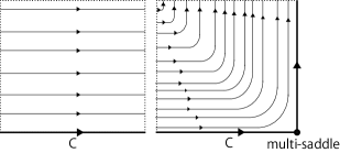
Figure 11. A flow box near a non-singular point and a flow box near a multi-saddle.

Since $\omega(x)\cap\gamma\neq\emptyset$, the $\omega$-limit set of a point in $\mathbb{A}$ is the semi-attracting limit circuit $C$. This means that $x\in\mathrm{int}\mathrm{P}(v)$ and so that $\omega(x)=C\subseteq\overline{\mathrm{int}\mathrm{P}(v)}\cap\gamma$ is a semi-attracting limit circuit. ∎

5.1. Surgeries for flows on surfaces

Recall that an invariant closed disk is a center disk if it is a union of one center and periodic orbits and is a neighborhood of the center. A closed disk is a sink (resp. source) disk if its boundary is a closed transversal and its interior consists of one sink (resp. source) and of orbit arcs of non-recurrent orbits (see Figure 12).

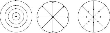
Figure 12. A center disk, a sink disk, and a source disk

Define an operation $\mathop{\mathrm{C}}_{o}$ as cutting an essential periodic orbit and pasting one or two center disks, an operation $\mathop{\mathrm{C}}_{d}$ as removing an essential one-sided (resp. two-sided) multi-saddle circuit and pasting a double covering (resp. two copies) of the multi-saddle circuit to the new boundary (resp. new two boundary components), and an operation $\mathop{\mathrm{C}}_{t}$ as cutting an essential closed transversal and pasting one sink disk and one source disk as in Figure 13.

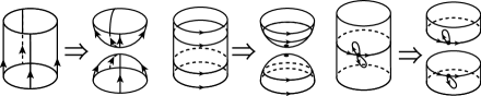
Figure 13. An operation $\mathop{\mathrm{C}}_{t}$, an operation $\mathop{\mathrm{C}}_{o}$, and an operation $\mathop{\mathrm{C}}_{d}$

A Cherry flow box is a disk with orbit arcs on the figure to the right in Figure 14.

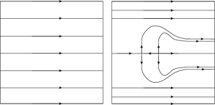
Figure 14. A flow box and a Cherry flow box

A Cherry blow-up operation is replacing a flow box with a Cherry flow box. Denote by $\mathop{\mathrm{Ch}}_{l}$ an inverse operation of a Cherry blow-up operation to a multi-saddle separatrix as shown in Figure 15.

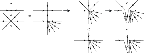
Figure 15. Inverse operation of a Cherry blow-up operation $\mathop{\mathrm{Ch}}_{l}$ to a separatrix from a $k$-saddle to a sink

Cutting essential parts, we can reduce surface flows into spherical flows.

Lemma 5.2.

Let $v$ be a quasi-regular flow on a connected compact surface $S$, $S_{o}$ the resulting surface from $S$ by applying an operation $\mathop{\mathrm{C}}_{o}$ as possible, $S_{d}$ the resulting surface from $S_{o}$ by applying an operation $\mathop{\mathrm{C}}_{d}$ as possible, and $S_{t}$ the resulting surface from $S_{d}$ by applying an operation $\mathop{\mathrm{C}}_{t}$ as possible. Then each connected component of the surface $S_{t}$ is a subset of a sphere up to homeomorphism.

Proof.

Removing ($\partial$-)$0$-saddles, we may assume that there are no ($\partial$-)$0$-saddles. Let $v_{o}$ be the resulting flow from $v$ on $S$, $v_{d}$ be the resulting flow on the resulting surface $S_{d}$ from $v_{o}$ on $S_{o}$, and $v_{t}$ be the resulting flow on the resulting surface $S_{t}$ from $v_{d}$ on $S_{d}$. Since $S$ is compact, the surface $S_{o}$ can be obtained by taking operations $C_{o}$ finitely many times. By construction, the flow $v_{o}$ has no essential periodic orbits. Since $S$ is compact, the surface $S_{d}$ can be obtained by taking operations $C_{d}$ finitely many times. By construction, the flow $v_{d}$ has neither essential periodic orbits nor essential loops in $D(v)$. Since $S_{d}$ is compact, the surface $S_{t}$ can be obtained by taking operations $C_{t}$ finitely many times. Then the flow $v_{t}$ has neither essential closed transversals, essential loops in $D(v)$, nor essential periodic orbits. Since each Q-set intersects some essential closed transversal, the flow $v_{t}$ has no Q-sets but consists of proper orbits. Replacing $\partial$-sinks (resp. $\partial$-sources) with pairs of a $\partial$-saddle and a sink (resp. a source) (see Figure 16), we may assume that there are neither $\partial$-sinks nor $\partial$-sources on $S_{t}$. Then each singular point on the boundary $\partial S_{t}$ is a multi-saddle. Let $S^{\prime}$ be the resulting closed surface from a connected component of $S_{t}$ by collapsing all boundary components into singletons and $v^{\prime}$ the resulting flow on $S^{\prime}$. By construction, it suffices to show that each connected component of $S^{\prime}$ is a subset of a sphere up to homeomorphism. Indeed, then each new singular point of $v^{\prime}$ is a multi-saddle. Quasi-regularity of $v$ implies that each singular point of the resulting flow $v^{\prime}$ is either a multi-saddle, a sink, a source, or a center. Since each limit circuit is not essential (i.e. either null homotopic or parallel to the boundary $\partial S^{\prime}$), collapsing disks each of whose boundary components is a limit circuit contained in the closure of an ss-separatrix into singletons and collapsing annuli $\mathbb{A}_{i}$ which are parallel to the boundary component of $S$ and whose boundary components $\partial\mathbb{A}_{i}\setminus\partial S$ outside of the boundary $\partial S^{\prime}$ are limit circuits contained in the closure of ss-separatrices into singletons, we may assume that there are no ss-separatrices whose $\omega$- or $\alpha$-limit sets are limit circuits and that there are no periodic orbits which are parallel to the boundary. Then each separatrix connecting a sink or a source does not belong to any multi-saddle connection, and each periodic orbit is null homotopic (i.e. contractible). For an ss-multi-saddle connection of $v^{\prime}$ with a $k$-saddle ($k>0$) such that there is a separatrix from a source to it (resp. from it to a sink), applying the inverse operation of $\mathop{\mathrm{Ch}}_{l}$ to the separatrix, we obtain an ss-multi-saddle connection with a $(k-1)$-saddle (see Figure  15). Applying the operations finitely many times and removing $0$-saddles, we may assume that there are no ss-separatrices connecting a multi-saddle and either a sink or a source. Therefore each semi-multi-saddle separatrix is a multi-saddle separatrix. Then each separatrix either connects a sink and a source or is contained in the multi-saddle connection diagram $D(v^{\prime})$ of $v^{\prime}$. By Lemma 5.1, the multi-saddle circuit is a limit circuit or is parallel to a periodic orbit. This means that each multi-saddle connection of $v^{\prime}$ is null homotopic. Collapsing closed disks each of whose boundary components is contained in the multi-saddle connection diagram $D(v^{\prime})$ into singletons, the new singletons are either centers, sinks, or sources. Thus we may assume that $D(v^{\prime})=\emptyset$ and that each periodic orbit is null homotopic. Therefore $v^{\prime}$ consists of sinks, sources, centers, non-recurrent orbits, and null homotopic periodic orbits. In particular the indices of singular points are positive if exists. If there are no singular points, then there are non-contractible periodic orbits or non-closed recurrent orbits, which contradicts non-existence of non-contractible periodic orbits and non-closed recurrent orbits. Thus there are singular points, whose indices are positive. Then the Euler characteristic is positive. Hence the Poincaré-Hopf theorem implies that each connected component of the surface $S^{\prime}$ is a sphere or a projective plane.

We show that each connected component of $S^{\prime}$ is a sphere. Otherwise there is a connected component $\mathbb{P}$ of $S^{\prime}$ is a projective plane. By the non-existence of multi-saddles, the Poincaré-Hopf theorem implies that there is a just one singular point on $\mathbb{P}$. Suppose that there is a center. Removing a small open center disk $B$, the complement $\mathbb{P}-B$ is a Möbius band without singular points and so their first return map to a transverse closed arc is an orientation-reversing homeomorphism on a closed interval. Then it has a unique fixed point which corresponds to a one-sided periodic orbit, which contradicts non-existence of essential periodic orbits. Suppose that there is a sink (resp. source). The Poincaré-Hopf theorem implies the $\alpha$-limit (resp. $\omega$-limit) set of each non-singular point is a periodic orbit. Since there is only one singular point, which is a sink (resp. source), there is a closed disk $B$ whose boundary is a periodic orbit and whose interior is the unstable manifold of the sink (resp. the stable manifold of the source) and so the complement $\mathbb{P}-\mathrm{int}B$ is a Möbius band without singular points, because the periodic orbit $\partial B$ is not essential. The same argument implies the contradiction.

Thus each connected component of $S_{t}$ is a subset of a sphere. ∎

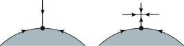
Figure 16. Replacing a $\partial$-sink with a pair of a sink and a $\partial$-saddle

Figure 17. A flow on a torus with heteroclinic multi-saddle separatrices but without essential closed transversals or essential periodic orbits

Note that the operation $\mathop{\mathrm{C}}_{d}$ is necessary in the previous lemma (see Figure 17).

5.2. Decomposition of quasi-regular flow using the strict border set

For a quasi-regular flow $v$ on a compact surface, recall that $\mathop{\mathrm{Bd}}(v)=\mathop{\mathrm{Sing}}(v)\sqcup\partial^{-}\mathop{\mathrm{Per}}(v)\sqcup\partial_{\mathop{\mathrm{Per}}(v)}\sqcup\mathop{\mathrm{P}_{\mathrm{semi}}}(v)\sqcup\mathop{\partial_{\mathrm{P}(v)}}\sqcup\mathrm{E}(v)$ is the union of singular points, the closure of the union of limit cycles, periodic orbits on $\partial S$, semi-multi-saddle separatrices, separatrices between a $\partial$-source and a $\partial$-sink on the boundary $\partial S$, and exceptional orbits. Since $\partial S\subseteq\mathop{\mathrm{Bd}}(v)$ for any quasi-regular flow $v$ on a compact surface $S$, we describe the complement of the strict border point set $\mathop{\mathrm{Bd}}(v)$ as follows.

Theorem 5.3.

Each connected component of $S-\mathop{\mathrm{Bd}}(v)$ for a quasi-regular flow $v$ on a compact surface $S$ is one of the following invariant open subsets exclusively:
$(1)$ A flow box in $\mathrm{P}(v)$, whose orbit space is an open interval,
$(2)$ An annulus in $\mathrm{P}(v)$, whose orbit space is a circle,
$(3)$ A torus in $\mathop{\mathrm{Per}}(v)$, whose orbit space is a circle,
$(4)$ A Klein bottle in $\mathop{\mathrm{Per}}(v)$, whose orbit space is an open interval,
$(5)$ An annulus in $\mathop{\mathrm{Per}}(v)$, whose orbit space is an interval,
$(6)$ A Möbius band in $\mathop{\mathrm{Per}}(v)$, whose orbit space is an interval, or
$(7)$ An essential subset in $\mathrm{LD}(v)$, whose orbit class space is a singleton.

Moreover, the following statements hold:
(a) The $\omega$-limit $(\mathrm{resp.}$ $\alpha$-limit$)$ set of a point in a connected component in $\mathrm{P}(v)\setminus\mathop{\mathrm{Bd}}(v)$ is the $\omega$-limit $(\mathrm{resp.}$ $\alpha$-limit$)$ set of any point in the connected component.
(b) The closure of a point in a connected component in $\mathrm{LD}(v)$ is the closure of any point in the connected component.
(c) The boundary $\partial O(x)$ of a point $x\in\mathrm{LD}(v)$ consists of finitely many multi-saddle separatrices and singular points.
(d) Any boundary component of a connected component of $S-\mathop{\mathrm{Bd}}(v)$ which does not intersect $\mathrm{E}(v)$ is a finite union of closed orbits and multi-saddle separatrices.

Proof.

Lemma 4.12 implies that the complement $S-\mathop{\mathrm{Bd}}(v)$ is open. Since the boundary $\partial S$ is contained in $\mathop{\mathrm{Bd}}(v)$, taking the double of a manifold if necessary, we may assume that $S$ is closed. We deform the flow $v$ on $S$ by following operations which preserve the complement $S-\mathop{\mathrm{Bd}}(v)$: Replacing each orbit in $\mathop{\partial_{\mathrm{P}(v)}}$ by a $\partial$-$0$-saddle with two ss-separatrices, we may assume that $\mathop{\partial_{\mathrm{P}(v)}}=\emptyset$. Replacing $\partial_{\mathop{\mathrm{Per}}(v)}$ with centers, we may assume that $\partial_{\mathop{\mathrm{Per}}(v)}=\emptyset$. Replacing $\partial$-sinks (resp. $\partial$-sources) with pairs of a $\partial$-saddle and a sink (resp. a source) as in Figure 16, we may assume that there are neither $\partial$-sinks nor $\partial$-sources.

Fix a connected component $U$ of $S-\mathop{\mathrm{Bd}}(v)$. Proposition 4.13 implies that the open subset $U$ is contained in either $\mathrm{int}\mathop{\mathrm{Per}}(v)$, $\mathrm{int}(\mathrm{P}(v)-\mathop{\mathrm{P}_{\mathrm{sep}}}(v))$, or $\mathrm{LD}(v)$. Suppose that $U\subseteq\mathrm{LD}(v)$. Since $\mathrm{LD}(v)$ is open, fix a point $x\in U$ and a transverse arc $I\subset U$ where $x$ is the interior point in $I$. Since $x$ is non-closed recurrent, by Lemma 3.5, taking a small transverse arc if necessary, by the waterfall construction, there is a closed transversal in $U$. By Lemma 3.6, the closed transversal is essential and so is $U$. Then $U$ is desired in the case $(7)$. Suppose that $U\subseteq\mathrm{int}\mathop{\mathrm{Per}}(v)$. If $\partial U=\emptyset$, then $U$ is either a torus or a Klein bottle and so is desired in the case $(3)$ or $(4)$. Thus we may assume that $\partial U\neq\emptyset$. Then $U$ is an open annulus or an open Möbius band and so is desired in the case $(5)$ or $(6)$. Suppose that $U\subseteq\mathrm{int}(\mathrm{P}(v)-\mathop{\mathrm{P}_{\mathrm{sep}}}(v))$. The $\omega$-limit (resp. $\alpha$-limit) set of each point in $U$ is either an exceptional Q-set, a limit circuit, or a sink (resp. a source). We deform the flow $v$ on $S$ by following operations which preserve $U$: Cutting an essential periodic orbit and pasting one or two center disks (i.e. taking operation $\mathop{\mathrm{C}}_{o}$), by induction, we may assume that each periodic orbit is null homotopic. Cutting limit cycles and collapsing the new boundary components into singletons if necessary, we may assume that there are no limit cycles on $\partial U$. Removing multi-saddle circuits in $\mathop{\mathrm{Bd}}(v)$, taking the metric completion, and collapsing the new boundary components into singletons, we may assume that there are no multi-saddle circuits in $\mathop{\mathrm{Bd}}(v)$, by replacing $S$ with the resulting surface $S_{\mathrm{col}}$. Here a new boundary component is a connected component of $S_{1}-(S-\Gamma)$ where $\Gamma$ is the union of multi-saddle circuits in $\mathop{\mathrm{Bd}}(v)$ and $S_{1}$ is the metric completion of $(S-\Gamma)$. In particular, there are neither limit circuits nor self-connected multi-saddle separatrices on $S$. By construction, new singletons are either sinks, sources, centers, or multi-saddles. Cutting the closures of multi-saddle separatrices and collapsing new boundary components into singletons, we may assume that there are no multi-saddle connection separatrices on $\partial U$. Note $U$ contains no multi-saddles. Then the $\omega$-limit (resp. $\alpha$-limit) set of each point in $U$ is either an exceptional Q-set or a sink (resp. a source).

Suppose that $\overline{U}\cap\mathrm{E}(v)=\emptyset$. The $\omega$-limit (resp. $\alpha$-limit) set of each point in $U$ is a sink (resp. a source). Fix a sink $s$ which is the $\omega$-limit set of a point in $U$ and a small closed transversal $\gamma$ which is a boundary of a sink disk of the sink $s$. If $\gamma$ is contained in $U$, then $U$ is an open annulus in $\mathrm{P}(v)$ and so is desired in the case $(2)$. Thus we may assume that $\gamma$ is not contained in $U$. Then there are separatrices $O_{i}$ between the sink $s$ and multi-saddles such that $O_{i}\subset\partial U$. Since each multi-saddle in $\partial U$ connects with a sink or a source, the boundary $\partial U$ consists of sinks, sources, multi-saddles, and semi-multi-saddle separatrices from sinks or to sources. Taking a double of $\overline{U}$ if necessary, the resulting flow on the resulting closed surface consists of sinks, sources, $0$-saddles, and non-recurrent orbits. Since the index of each singular point is non-negative, the existence of both a sink and a source and the Poincaré-Hopf theorem imply that the double is a sphere and there are exactly one sink and one source except $0$-saddles on the double. This means $U$ is an invariant open flow box in $\mathrm{P}(v)$ and so is desired in the case $(1)$.

Thus we may assume that $\overline{U}\cap\mathrm{E}(v)\neq\emptyset$. This implies that $S$ is not spherical. We deform the flow $v$ on $S$ by following operations which preserve $U$: Applying an operation $\mathop{\mathrm{C}}_{d}$ as possible, we may assume that the flow $v$ has neither essential periodic orbits nor essential loops in $D(v)$. Cutting an essential closed transversal in $\mathrm{LD}(v)$ and pasting one sink disk and one source disk, we may assume that $\mathrm{LD}(v)=\emptyset$.

We show that $U$ is an invariant flow box in $\mathrm{P}(v)$ desired in the case $(1)$, by cutting $U$ into small open flow boxes. Indeed, cutting an essential closed transversal $\gamma_{i}$ intersecting $\mathrm{E}(v)$ and pasting one sink disk and one source disk (i.e. applying an operation $\mathop{\mathrm{C}}_{t}$) as possible, let $T$ be the resulting surface from $S$, $w$ the resulting flow, and $U^{-}\subseteq T$ the resulting subset of $U\setminus\bigcup_{i}\gamma_{i}$. By Lemma 5.2, the resulting surface $T$ is spherical. Let $U_{k}$ be the connected components of $U^{-}$ with $U^{-}=\bigsqcup_{k}U_{k}$. Denote by $\widetilde{U}$ (resp. $\widetilde{U}_{k}$) the saturation of $U^{-}$ (resp. $U_{k}$) by $w$. By construction, each connected component $\widetilde{U}_{k}$ of $\widetilde{U}$ is an open flow box such that $\omega(x)=a$ and $\alpha(x)=b$ for the new sink $a$ and the new source $b$. Then each connected component $U_{k}$ of $U\setminus\bigcup_{i}\gamma_{i}$ is an invariant open flow box each of whose vertical boundary components is a closed interval in an essential closed transversal $\gamma_{i}$. In other words, each connected component $U_{k}$ has one $\alpha$-vertical boundary and one $\omega$-vertical boundary. Since $U$ is constructed by pasting one $\alpha$-vertical boundary and one $\omega$-vertical boundary of $U_{k}$ as possible, we have $U$ is an invariant open flow box in $\mathrm{P}(v)$ and so is desired in the case $(1)$. This complete the classification of connected components of the complement $S-\mathop{\mathrm{Bd}}(v)$.

By Proposition 4.14, the strict border point set $\mathop{\mathrm{BD}}(v)$ consists of singular points, one-sided periodic orbits, semi-multi-saddle separatrices, separatrices on $\partial S$ between $\partial$-sources and $\partial$-sinks, the closure of the union of limit cycles, and finitely many exceptional Q-sets. Moreover, the union $\mathop{\mathrm{Bd}}(v)\sqcup\mathrm{LD}(v)$ consists of finitely many orbit classes. Then the set difference $\mathop{\mathrm{Bd}}(v)-\mathrm{E}(v)$ consists of finitely many proper orbits. Fix a connected component $U$ of $(\mathrm{P}(v)\sqcup\mathrm{LD}(v))\setminus\mathop{\mathrm{BD}}(v)$ and a point $x\in U$. Suppose that $x\in\mathrm{LD}(v)$. Proposition 2.2 [47] implies that $U\subseteq\mathrm{LD}(v)$ and $\overline{O(x)}=\overline{O(y)}$ for any $y\in U$. This implies the assertion (b). Lemma 3.2 and Proposition 4.5 imply that the intersection $\mathop{\mathrm{BD}}(v)\cap\partial^{+}\overline{O(x)}\subseteq\partial^{+}\mathrm{LD}(v)\subseteq\partial^{-}\mathop{\mathrm{Sing}}(v)\sqcup\partial^{-}\mathrm{P}(v)$ consists of finitely many multi-saddle separatrices and singular points. This implies the assertion (c). Thus we may assume that $x\in\mathrm{P}(v)\setminus\mathop{\mathrm{BD}}(v)$. Suppose that $\omega(x)\cap\mathrm{E}(v)\neq\emptyset$. Then $U$ is an invariant flow box. By the construction above, the $\omega$-limit sets of any point in $U$ is the exceptional Q-set $\omega(x)$. Thus we may assume that $\bigcup_{y\in U}\omega(y)\cap\mathrm{E}(v)=\emptyset$. By symmetry, we may assume that $\bigcup_{y\in U}\alpha(y)\cap\mathrm{E}(v)=\emptyset$. From Poincaré-Bendixson theorem for a flow with finitely many singular points, the $\omega$-limit set $\omega(y)$ of any point $y\in U$ is either a sink, a $\partial$-sink, or a semi-attracting limit circuit. By the flow fox theorem, the $\omega$-limit set $\omega(z)$ of each point $z$ in some small neighborhood of any point $y\in U$ corresponds to $\omega(y)$. The open condition implies that the $\omega$-limit set $\omega(y)$ of any point $y\in U$ corresponds to $\omega(x)$. By symmetry, the $\alpha$-limit set $\alpha(y)$ of any point $y\in U$ corresponds to $\alpha(x)$. This implies the assertion (a).

By Lemma 4.12, we obtain $\mathop{\mathrm{BD}}(v)-\mathrm{E}(v)=\mathop{\mathrm{Sing}}(v)\sqcup\partial^{-}\mathop{\mathrm{Per}}(v)\sqcup\partial_{\mathop{\mathrm{Per}}(v)}\sqcup\mathop{\mathrm{Per}}_{1}(v)\sqcup\partial^{-}\mathrm{P}(v)\sqcup\mathop{\mathrm{P}_{\mathrm{sep}}}(v)$. Let $U$ be a connected component of $S-\mathop{\mathrm{Bd}}(v)$ and $\partial$ a connected component of $\partial U$ with $\mathrm{E}(v)\cap\partial=\emptyset$. Then $\partial\subseteq\mathop{\mathrm{BD}}(v)-\mathrm{E}(v)=\mathop{\mathrm{Sing}}(v)\sqcup\partial^{-}\mathop{\mathrm{Per}}(v)\sqcup\partial_{\mathop{\mathrm{Per}}(v)}\sqcup\mathop{\mathrm{Per}}_{1}(v)\sqcup\partial^{-}\mathrm{P}(v)\sqcup\mathop{\mathrm{P}_{\mathrm{sep}}}(v)$. If $\mathop{\mathrm{Per}}(v)\cap\partial\neq\emptyset$, then the connectivity of $\partial$ implies that $\partial$ is a periodic orbit and so that the assertion (d) holds. Thus we may assume that $\partial\subseteq\mathop{\mathrm{Sing}}(v)\sqcup\partial^{-}\mathrm{P}(v)\sqcup\mathop{\mathrm{P}_{\mathrm{sep}}}(v)$. From Lemma 4.12, the union $\mathop{\mathrm{Sing}}(v)\sqcup\partial^{-}\mathrm{P}(v)\sqcup\mathop{\mathrm{P}_{\mathrm{sep}}}(v)$ is a finite union of singular points and multi-saddle separatrices. Therefore the assertion (d) holds. ∎

5.3. Proof of Theorem A

Let $v$ be a regular-like flow on a compact surface $S$. By Lemma 4.15, we have $\mathop{\mathrm{Bd}}(v)-\mathop{\mathrm{Bd}}_{0}(v)=\partial_{\mathop{\mathrm{Per}}(v)}\sqcup\mathop{\partial_{\mathrm{P}(v)}}$. Therefore Theorem A is followed from Theorem 5.3.

5.4. Description of components of the decompositions and their boundaries

5.4.1. Vertical boundary of an invariant open subset by flows

For an invariant open subset $A$, define the vertical boundary $\partial_{\perp}A$ of $A$ as follows:

$$\partial_{\perp}^{\alpha}A:=(\bigcup_{x\in A}\alpha(x))\setminus A$$

$$\partial_{\perp}^{\omega}A:=(\bigcup_{x\in A}\omega(x))\setminus A$$

$$\partial_{\perp}A:=\partial_{\perp}^{\alpha}A\cup\partial_{\perp}^{\omega}A$$

We call that $\partial_{\perp}^{\alpha}A$ (resp. $\partial_{\perp}^{\omega}A$, $\partial_{\perp}A$) is the $\alpha$-vertical (resp. $\omega$-vertical, vertical) boundary. For an oriented invariant flow box $B\cong\mathbb{D}$, the $\alpha$-vertical (resp. $\omega$-vertical) boundary $\partial_{\perp}^{\alpha}B$ (resp. $\partial_{\perp}^{\omega}B)$ is the boundary component of $\partial_{\perp}B$ corresponding to $\{0\}\times(0,1)$ (resp. $\{1\}\times(0,1)$) (see the figure to the left in Figure 18).

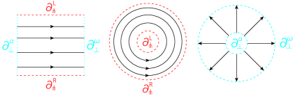
Figure 18. A flow box, a periodic annulus, and an open transverse annulus

For an open periodic annulus $B\cong\mathbb{A}_{\widetilde{+}}$, the vertical boundary components are empty (i.e. $\partial_{\perp}^{\alpha}B=\partial_{\perp}^{\omega}B:=\emptyset$). For an open transverse annulus $B\cong\mathbb{A}$, the $\alpha$-vertical (resp. $\omega$-vertical) boundary $\partial_{\perp}^{\alpha}B$ (resp. $\partial_{\perp}^{\omega}B)$ is the boundary component of $\partial_{\perp}B$ corresponding to $\{(\cos\theta,\sin\theta)\mid\theta\in[0,2\pi]\}$ (resp. $\{(2\cos\theta,2\sin\theta)\mid\theta\in[0,2\pi]\}$) (see the figure to the right in Figure 18).

5.4.2. $\alpha^{\prime}(x)$-limit sets and $\omega^{\prime}$-limit sets of points and orbits

Define $\alpha^{\prime}(x)$ and $\omega^{\prime}(x)$ for a point $x\in X$ as follows [5, 22]:

$$\alpha^{\prime}(x):=\alpha(x)\setminus O(x)$$

$$\omega^{\prime}(x):=\omega(x)\setminus O(x)$$

We call $\alpha^{\prime}(x)$ the $\alpha^{\prime}$-limit set of $x$ and $\omega^{\prime}(x)$ the $\omega^{\prime}$-limit set of $x$. For a subset $A\subseteq S$, define $\alpha^{\prime}(A)$ and $\omega^{\prime}(A)$ as follows:

$$\alpha^{\prime}(A):=\bigcup_{x\in A}\alpha^{\prime}(x)$$

$$\omega^{\prime}(A):=\bigcup_{x\in A}\omega^{\prime}(x)$$

Then $\alpha^{\prime}(O)=\alpha(O)\setminus O$ and $\omega^{\prime}(O)=\omega(O)\setminus O$ for an orbit $O$. As mentioned, the definition of $\alpha^{\prime}(p)$ (resp. $\omega^{\prime}(p)$) by Buendía and Lópes is slightly different from the original one, cf. [22, 26, 27] but these definitions correspond for proper orbits. Note that an orbit $O$ is closed if and only if $\alpha^{\prime}(O)=\emptyset$ (resp. $\omega^{\prime}(O)=\emptyset$). Since flows of finite type have no non-proper orbits, two definition of $\alpha^{\prime}(p)$ (resp. $\omega^{\prime}(p)$) by Buendía and Lópes and by the original one, cf. [22, 26, 27] correspond to each other for flows of finite type.

5.4.3. Transverse boundary of an invariant open subset by flows

Recall that a subset is locally connected if each point in it have a small open connected neighborhood. For an invariant open subset $A$ with locally connected boundary, define the transverse boundary $\partial_{\pitchfork}A$ of $A$ as follows: Put $\Gamma:=\bigcup_{x\in A}\alpha^{\prime}(x)\cup\omega^{\prime}(x)$. Let $S_{1}$ be the metric completion of $S-\Gamma$, $\partial:=S_{1}-(S-\Gamma)$ the new boundary of $S_{1}$, and $\pi:S_{1}\to S$ the natural continuous surjection associated to the metric completion such that a restriction $\pi|_{\partial}:\partial\to\Gamma$ is an immersion except singular points and a restriction $\pi_{S_{1}-\partial}:S_{1}-\partial\to S-\Gamma$ is an identity mapping. Here a mapping $f$ is an immersion except singular points if the restriction to the complement of the inverse image of the singular point set is injective. Then we define

$$\partial_{\pitchfork}A:=\pi\left(\partial_{S_{1}}A-(\alpha^{\prime}_{v_{1}}(A)\cup\omega^{\prime}_{v_{1}}(A))\right)=\pi\left(\partial_{S_{1}}A-\bigcup_{x\in A}(\alpha^{\prime}_{v_{1}}(x)\cup\omega^{\prime}_{v_{1}}(x))\right)$$

where $v_{1}$ is the resulting flow on $S_{1}$ induced by $v$, $\partial_{S_{1}}A$ is the boundary of $A$ in $S_{1}$, $\alpha^{\prime}_{v_{1}}(x)$ is the $\alpha^{\prime}$-limit set of $x$ with respect to $v_{1}$, and $\omega^{\prime}_{v_{1}}(x)$ is the $\omega^{\prime}$-limit set of $x$ with respect to $v_{1}$. Note that $\partial_{\pitchfork}A\cap\partial_{\perp}A\neq\emptyset$ in general and that metric completions are necessary to define the transverse boundary. In fact, there is a flow on an orientable closed surface $\Sigma_{2}$ with genus two which consists of two singular points $x_{1}$ and $x_{2}$ and non-recurrent orbits with the strict border point set $\mathop{\mathrm{BD}}(v)=\bigsqcup_{i=1}^{2}x_{i}\sqcup\bigsqcup_{i=1}^{5}O_{i}$ such that the complement $\Sigma_{2}-\mathop{\mathrm{BD}}(v)$ is an invariant flow box $U$ as in Figure 19 with $\partial_{\pitchfork}U\cap\partial_{\perp}U=\bigsqcup_{i=1}^{2}x_{i}\sqcup\bigsqcup_{i=1}^{2}O_{i}\neq\emptyset$ and $\partial_{\pitchfork}U=\bigsqcup_{i=1}^{2}x_{i}\sqcup\bigsqcup_{i=1}^{5}O_{i}\supsetneq O_{3}\sqcup O_{4}\sqcup O_{5}=\partial U-\bigcup_{x\in U}(\alpha^{\prime}(x)\cup\omega^{\prime}(x))=\partial U-\partial_{\perp}U$.

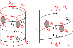
Figure 19. A flow on an orientable closed surface with genus two is obtained by glueing a pair of two circuits labelled by $x_{1}\sqcup O_{1}$ and a pair of two circuits labelled by $x_{2}\sqcup O_{2}$.

5.4.4. Left and right transverse boundary components of canonical regions

Let $v$ be a quasi-regular flow with $\mathrm{E}(v)=\emptyset$ on a compact surface. For an oriented invariant flow box $B\cong\mathbb{D}$, denote by $\partial_{\pitchfork}^{L}B$ (resp. $\partial_{\pitchfork}^{R}B)$ the image by the mapping $\pi$ in the previous subsection of the boundary component of $\partial_{S_{1}}B-(\alpha^{\prime}_{v_{1}}(B)\cup\omega^{\prime}_{v_{1}}(B))$ corresponding to $(0,1)\times\{0\}$ (resp. $(0,1)\times\{1\}$) (see the figure to the left in Figure 18). By definition, we have $\partial_{\pitchfork}B=\partial_{\pitchfork}^{L}B\cup\partial_{\pitchfork}^{R}B$. For an open periodic annulus $B\cong\mathbb{A}$, denote by $\partial_{\pitchfork}^{L}B$ (resp. $\partial_{\pitchfork}^{R}B)$ the boundary component of $\partial_{\pitchfork}B$ corresponding to $\{(\cos\theta,\sin\theta)\mid\theta\in[0,2\pi]\}$ (resp. $\{(2\cos\theta,2\sin\theta)\mid\theta\in[0,2\pi]\}$) (see the figure to the middle in Figure 18). For an open transverse annulus $B\cong\mathbb{A}_{\widetilde{+}}$, define $\partial_{\pitchfork}^{L}B=\partial_{\pitchfork}^{R}B:=\emptyset$. We call that $\partial_{\pitchfork}^{R}B$ (resp. $\partial_{\pitchfork}^{L}B$) is the right (resp. left) transverse boundary.

5.4.5. Description of transverse and vertical boundaries

Theorem 5.3 implies the following statements.

Corollary 5.4.

Each connected component of $S-\mathop{\mathrm{BD}}(v)$ for a quasi-regular flow $v$ on a compact surface $S$ is one of the following invariant open subsets exclusively:
$(1)$ A flow box in $\mathrm{P}(v)$, whose orbit space is an interval,
$(2)$ An annulus in $\mathrm{P}(v)$, whose orbit space is a circle,
$(3)$ A torus in $\mathop{\mathrm{Per}}(v)$, whose orbit space is a circle,
$(4)$ An annulus in $\mathop{\mathrm{Per}}(v)$, whose orbit space is an interval, or
$(5)$ An essential subset in $\mathrm{LD}(v)$, whose orbit class space is a singleton.

Moreover, the following statements hold:
(a) The $\omega$-limit $(\mathrm{resp.}$ $\alpha$-limit$)$ set of a point in a connected component in $\mathrm{P}(v)\setminus\mathop{\mathrm{BD}}(v)$ is the $\omega$-limit $(\mathrm{resp.}$ $\alpha$-limit$)$ set of any point in the connected component.
(b) The closure of a point in a connected component in $\mathrm{LD}(v)$ is the closure of any point in the connected component.
(c) Each of the vertical $\alpha$- and $\omega$-vertical boundaries of any connected components of $S-\mathop{\mathrm{BD}}(v)$ in the case $(1)$ and $(2)$ is an immersed line which is a finite union of closed orbits and multi-saddle separatrices.
(d) Each of the left and right transverse boundaries of any connected components of $S-\mathop{\mathrm{BD}}(v)$ in the case $(1)$ and $(4)$ is an immersed line which is a finite union of closed orbits and multi-saddle separatrices unless the left/right transverse boundary intersects $\mathrm{E}(v)$.

For a non-quasi-regular flow $v$ on a compact surface, note that the left and right transverse boundaries of connected components of the complement of the border point set $\mathop{\mathrm{BD}}(v)$ in the case $(1)$ and $(4)$ in the previous corollary are not connected in general and that the $\omega$-limit sets of points in the domain are different from each other in general (see Figure 20).

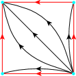
Figure 20. The complement of the border point set $\mathop{\mathrm{BD}}(v)$ in a closed disk is an open disk whose left (resp. right) transverse boundary is a disjoint union of two open intervals and whose $\omega$-vertical boundary consists of three points such that each $\omega$-limit set is a singular point.

5.4.6. Description of components of the decompositions

Recall that a quasi-regular flow without recurrent points ($\mathrm{i.e.}$ $\mathrm{LD}(v)\sqcup\mathrm{E}(v)=\emptyset$) is of finite type if there are at most finitely many limit cycles. In the finite type case, we obtain the following statement from Proposition 4.17, Theorem 5.3, and Corollary 5.4.

Proposition 5.5.

The following statements hold for a flow $v$ of finite type on a compact surface $S$:
$(1)$ The orbit spaces $(S-\mathop{\mathrm{Bd}}(v))/v$ and $(S-D_{\mathrm{ss}}(v))/v$ are finite disjoint unions of intervals and circles.
$(2)$ The orbit space $(S-\mathop{\mathrm{BD}}(v))/v$ is a finite disjoint union of open intervals and circles.

Moreover, the boundary of each connected component of $S-\mathop{\mathrm{BD}}(v)$ is a finite union of closed orbits and separatrices.

5.5. Proof of Theorem B

Let $v$ be a regular-like flow on a compact surface $S$. By Lemma 4.15, we have $\mathop{\mathrm{BD}}(v)-\mathop{\mathrm{BD}}_{0}(v)=\mathop{\partial_{\mathrm{P}(v)}}$. Therefore Theorem B is followed from Proposition 4.17 and Corollary 5.4.

5.6. Applications to Hamiltonian flows

Recall that denote by $\mathop{\mathrm{Sing}_{c}}(v)$ the set of centers. We have the following properties.

Corollary 5.6.

The following statements hold for any Hamiltonian flow $v$ with finitely many singular points on a compact surface $S$:
(1) The flow $v$ is of finite type.
(2) The strict border point set $\mathop{\mathrm{Bd}_{0}}(v)=D(v)\sqcup\mathop{\mathrm{Sing}_{c}}(v)$ is the finite union of centers, multi-saddles, and multi-saddles separatrices
(3) The complement $S-\mathop{\mathrm{Bd}_{0}}(v)$ is the finite union of invariant open periodic annuli.

Proof.

From the existence of Hamiltonian, the surface $S$ is orientable and contains neither periodic tori, periodic Möbius bands nor periodic Klein bottles. Moreover, Lemma 4.4 implies that the open invariant union $\mathrm{LD}(v)$ of locally dense orbits is empty. Since any Hamiltonian flow on a surface is volume-preserving and so has no wandering domains, the flow $v$ has no wandering domain and so is non-wandering. Theorem 3 [7] implies that $v$ is quasi-regular. By Lemma 4.15, we obtain $\mathop{\mathrm{Bd}}(v)-\mathop{\mathrm{Bd}}_{0}(v)=\partial_{\mathop{\mathrm{Per}}(v)}$. The non-existence of wandering domains implies that there are no limit circuits, the interior of the union $\mathrm{P}(v)$ of non-recurrent orbits is empty. Lemma 4.7 implies that $\mathrm{E}(v)=\emptyset$. This means that $v$ is of finite type and $S=\mathop{\mathrm{Cl}}(v)\sqcup\mathrm{P}(v)=\overline{\mathop{\mathrm{Per}}(v)}$. Theorem 5.3 implies that each connected component of $S-\mathop{\mathrm{Bd}}(v)$ is an invariant open periodic annulus and that $\mathop{\mathrm{Bd}}(v)$ is the finite union of centers, multi-saddles, and multi-saddles separatrices. From Proposition 5.5, the finiteness of $\mathop{\mathrm{Bd}_{0}}(v)$ and its complement hold. This means that the assertions (2)–(3) hold. ∎

The previous corollary means that any Hamiltonian flow with finitely many singular points on a compact surface can be obtained by glueing the boundaries of finitely many invariant open periodic annuli.

5.7. Applications to Morse-Smale flows

Recall that, under three generic conditions for differentials to guarantee structural stability, Labarca and Pacifico defined a Morse-Smale vector field on a compact manifold as follows [15]. A $C^{\infty}$ vector field $X$ on a compact manifold is Morse-Smale if $(1)$ the non-wandering set $\Omega(X)$ consists of finitely many hyperbolic closed orbits; $(2)$ the restriction $X|_{\partial M}$ is Morse-Smale; $(3)$ for any orbits $O,O^{\prime}\subset\Omega(X)$ and for any non-transversal point $x\in W^{s}(O)\cap W^{u}(O^{\prime})$, we have $x\in\partial M$ and either $O$ or $O^{\prime}$ is singular with respect to $X$ (i.e. $O\subseteq\mathop{\mathrm{Sing}}(X)$ or $O^{\prime}\subseteq\mathop{\mathrm{Sing}}(X)$). Therefore we say that a flow on a compact manifold is Morse-Smale if it is topologically equivalent to a flow generated by a Morse-Smale vector field. Note that the two generic conditions for differentials form an open dense subset of the set of $C^{\infty}$ vector fields and that they are stated as follows: any closed orbit is $C^{2}$ linearizable, and the weakest contraction (resp. expansion) at any closed orbit is defined. Here the weakest contraction at a singular (resp. periodic) point $p$ is defined if the contractive eigenvalue with biggest real part among the contractive eigenvalues of $DX(p)$ (resp. $DX_{f}(p)$, where $X_{f}$ is the Poincaré map) is simple. Dually we can define that the weakest expansion at p is defined. Under the $C^{2}$ linearizable condition and the eigenvalue conditions, a Morse-Smale $C^{\infty}$ vector field on a compact manifold is structurally stable with respect to the set of $C^{\infty}$ vector fields [15]. Any Morse-Smale flow on a compact surface can be obtained by glueing the boundaries of finitely many transverse annuli and invariant flow boxes as follows.

Corollary 5.7.

The following statements hold for any Morse-Smale flow $v$ on a compact surfaces $S$:
(1) The flow $v$ is of finite type.
(2) The strict border point set $\mathop{\mathrm{Bd}_{0}}(v)=D_{\mathrm{ss}}(v)$ is the finite union of sources, $\partial$-sources, sinks, $\partial$-sinks, saddles, $\partial$-saddles, limit cycles, and semi-multi-saddle separatrices.
(3) The complement $S-\mathop{\mathrm{Bd}_{0}}(v)$ is the finite union of invariant transverse annuli and invariant flow boxes.

Proof.

By definition, the closed point set $\mathop{\mathrm{Cl}}(v)$ consists of finitely many sources, $\partial$-sources, sinks, $\partial$-sinks, saddles, $\partial$-saddles, and limit cycles and we have $S=\mathop{\mathrm{Cl}}(v)\sqcup\mathrm{P}(v)=\overline{\mathrm{P}(v)}$. Therefore the flow $v$ is of finite type. By Lemma 4.15, we have $\mathop{\mathrm{Bd}}(v)-\mathop{\mathrm{Bd}}_{0}(v)=\mathop{\partial_{\mathrm{P}(v)}}$. Theorem 5.3 implies that each connected component of $S-\mathop{\mathrm{Bd}}(v)$ is either an invariant open transverse annulus or an invariant open flow box and so that so is one of $S-\mathop{\mathrm{Bd}_{0}}(v)$. From Proposition 5.5, the finiteness of $\mathop{\mathrm{Bd}_{0}}(v)$ and its complement holds. The non-degeneracy of singular points implies that the union $\mathop{\mathrm{P}_{\mathrm{semi}}}(v)$ consists of semi-multi-saddle separatrices. Therefore $\mathop{\mathrm{Bd}_{0}}(v)=\mathop{\mathrm{Sing}}(v)\sqcup\partial^{-}\mathop{\mathrm{Per}}(v)\sqcup\mathop{\mathrm{P}_{\mathrm{semi}}}(v)=\mathop{\mathrm{Cl}}(v)\sqcup\mathop{\mathrm{P}_{\mathrm{semi}}}(v)=D_{\mathrm{ss}}(v)$ is desired. ∎

6. Enumeration of flows of finite type

6.1. On the (strictly) border point set

Recall several concepts to describe the combinatorial structures of the (strictly) border point sets and their complements of flows of finite type.

6.1.1. Graphs

Recall an ordered triple $G:=(V,E,r)$ is an abstract multi-graph if $V$ and $E$ are sets and $r:E\to\{\{x,y\}\mid x,y\in V\}$. A graph is a cell complex whose dimension is at most one and which is a geometric realization of an abstract multi-graph.

6.1.2. Orders

A binary relation $\leq$ on a set $P$ is a pre-order if it is reflexive (i.e. $a\leq a$ for any $a\in P$) and transitive (i.e. $a\leq c$ for any $a,b,c\in P$ with $a\leq b$ and $b\leq c$). For a pre-order $\leq$, the inequality $a<b$ means both $a\leq b$ and $a\neq b$. A pre-order $\leq$ on $X$ is a partial order if it is antisymmetric (i.e. $a=b$ for any $a,b\in P$ with $a\leq b$ and $b\leq a$). A poset is a set with a partial order. For a point $x$ of a pre-ordered set $P$, define the class $\hat{x}:=\{y\in P\mid x\leq y,y\leq x\}$. The set of classes of a pre-ordered set $P$ is a decomposition and so its quotient space is a poset with respect to the induced order, which is called the class space of $P$ and denoted by $\hat{P}$. A pre-order order $\leq$ is a total order (or linear order) if either $a<b$ or $b<a$ for any points $a\neq b$.

6.1.3. Specialization pre-orders of topologies

The specialization pre-order $\leq_{\tau}$ on a topological space $(X,\tau)$ is defined as follows: $x\leq_{\tau}y$ if $x\in\overline{\{y\}}$. Then the class $\hat{x}=\{y\in X\mid\in\overline{\{y\}}$ of a point $x\in X$. The class space with the quotient topology is a $T_{0}$ space, which is called the $T_{0}$-tification of $X$ and denoted by $\hat{X}$.

6.1.4. Multi-graphs

Recall that a graph is a cell complex whose dimension is at most one and which is a geometric realization of an abstract multi-graph. In other words, it can be drawn such that no edges cross each other. Such a drawing is called a surface (directed) graph. Note that a finite (directed) multi-graph can be embedded in some surface. Moreover we call that a disjoint union of a surface directed graph and finite simple closed directed curves embedded in a surface is a generalized surface directed graph. We say that an ordered triple $G=(V,E,r)$ is an abstract multi-graph with $0$-hyper-edges if $V$ and $E$ are sets and $r:E\to\{\{x,y\}\mid x,y\in V\}\sqcup\{\emptyset\}$. Note that a generalized surface directed graph is a geometric realization of an abstract multi-graph with $0$-hyper-edges on a surface such that $0$-hyper-edges are realized by disjoint simple closed directed curves.

6.1.5. Multi-graphs as posets

A poset $P$ is said to be multi-graph-like if the height of $P$ is at most one and $|\overline{\{x\}}|\leq 3$ for any element $x\in P$. For a multi-graph-like poset $P$, each element of $P_{0}$ is called a vertex, and each element of $P_{1}$ is called an edge. Then an abstract multi-graph $G$ can be considered as a multi-graph-like poset $(P,\leq_{G})$ with $V=P_{0}$ and $E=P_{1}$ as follows: $P=V\sqcup\mathrm{E}(v)$ and $x<_{G}e$ if $x\in r(e)$. Conversely, a multi-graph-like poset $P$ can be considered as an abstract multi-graph with $V=P_{0}$, $E=P_{1}$, and $r:P_{1}\to\{\{x,y\}\mid x,y\in V\}$ defined by $r(e):=\partial^{+}\{e\}=\overline{\{e\}}-\{e\}$.

6.1.6. Extended orbits

Let $v$ be a flow on a compact connected surface $S$. Define a relation $\sim_{\mathrm{ex}}$ on $S$ as follows: $x\sim_{\mathrm{ex}}y$ if either $O(x)=O(y)$ or both $x$ and $y$ are contained in a multi-saddle connection. Write the extended orbit space $S/v_{\mathrm{ex}}:=S/\sim_{\mathrm{ex}}$. In other words, $S/v_{\mathrm{ex}}$ can be obtained from $S/v$ by collapsing the multi-saddle connections into singletons. Note that $(S-\mathop{\mathrm{Bd}}(v))/v=(S-\mathop{\mathrm{Bd}}(v))/v_{\mathrm{ex}}$ and that each class of $\sim_{\mathrm{ex}}$ is either an orbit or a multi-saddle connection. Denote by $S/\hat{v}_{\mathrm{ex}}$ the $T_{0}$-tification of $S/v_{\mathrm{ex}}$, called the extended orbit class space. In other words, define a relation $\approx_{\mathrm{ex}}$ on $S$ as follows: $x\approx_{\mathrm{ex}}y$ if either $\overline{O(x)}=\overline{O(y)}$ or both $x$ and $y$ are contained in a multi-saddle connection. Then $S/\hat{v}_{\mathrm{ex}}:=S/\approx_{\mathrm{ex}}$. By Proposition 2.2 [47] and Corollary 3.4 [48], the definitions of the equivalences $\sim_{\mathrm{ex}}$ and $\approx_{\mathrm{ex}}$ imply the following lemma.

Lemma 6.1.

Let $v$ be a flow on a compact connected surface $S$. The following conditions are equivalent:
$(1)$ $S/\hat{v}_{\mathrm{ex}}=S/v_{\mathrm{ex}}$.
$(2)$ $S/\hat{v}=S/v$.
$(3)$ $\mathrm{LD}(v)\sqcup\mathrm{E}(v)=\emptyset$ $(\mathrm{i.e.}$ each recurrent orbit is closed$)$.
$(4)$ $S/v$ is $T_{0}$.
$(5)$ Each orbit is proper.

6.2. Finiteness and Enumerability of flows of finite type

We obtain the finiteness of the strict border point sets.

Proposition 6.2.

Let $v$ be a flow of finite type on a compact connected surface $S$. The following statements hold:
$(1)$ The quotient space $\mathop{\mathrm{Bd}}(v)/\hat{v}_{\mathrm{ex}}=\mathop{\mathrm{Bd}}(v)/v_{\mathrm{ex}}$ is a finite abstract multi-graph $(V_{\mathop{\mathrm{Bd}}(v)},E_{\mathop{\mathrm{Bd}}(v)})$ such that the vertex set $V_{\mathop{\mathrm{Bd}}(v)}$ consists of centers, periodic orbits on $\partial S$, multi-saddle connections, sinks, $\partial$-sinks, sources, $\partial$-sources, and limit cycles, and that the edge set $E_{\mathop{\mathrm{Bd}}(v)}$ consists of ss-separatrices and non-closed orbits on $\partial S$ connecting $\partial$-sinks and $\partial$-sources.

Proof.

By Lemma 6.1, we obtain $\mathop{\mathrm{Bd}}(v)/\hat{v}_{\mathrm{ex}}=\mathop{\mathrm{Bd}}(v)/v_{\mathrm{ex}}$. Proposition 4.14 implies that the strict border point set $\mathop{\mathrm{Bd}}(v)=\mathop{\mathrm{BD}}(v)-\mathop{\mathrm{Per}}_{1}(v)$ is the finite union of singular points, periodic orbits on the boundary $\partial S$, semi-multi-saddle separatrices, separatrices between a $\partial$-source and a $\partial$-sink on $\partial S$, and limit cycles. Let $E_{\mathop{\mathrm{Bd}}(v)}$ be the union of ss-separatrices and separatrices between a $\partial$-source and a $\partial$-sink on the boundary $\partial S$. Then $E_{\mathop{\mathrm{Bd}}(v)}=(\mathop{\mathrm{P}_{\mathrm{semi}}}(v)\setminus D(v))\sqcup\mathop{\partial_{\mathrm{P}(v)}}=(\mathop{\mathrm{P}(v)_{\mathrm{ms}}}\sqcup\mathop{\mathrm{P}(v)_{\mathrm{ss}}}\sqcup\partial^{-}\mathrm{P}(v)\sqcup\mathop{\partial_{\mathrm{P}(v)}})\setminus D(v)$. Put $V_{\mathop{\mathrm{Bd}}(v)}:=\mathop{\mathrm{Bd}}(v)-E_{\mathop{\mathrm{Bd}}(v)}$. Since $\mathop{\mathrm{Bd}}(v)=\mathop{\mathrm{Sing}}(v)\sqcup\partial_{\mathop{\mathrm{Per}}(v)}\sqcup\partial^{-}\mathop{\mathrm{Per}}(v)\sqcup\partial^{-}\mathrm{P}(v)\sqcup\mathop{\mathrm{P}_{\mathrm{sep}}}(v)$, we have $V_{\mathop{\mathrm{Bd}}(v)}=(\mathop{\mathrm{Sing}}(v)\sqcup\partial_{\mathop{\mathrm{Per}}(v)}\sqcup\partial^{-}\mathop{\mathrm{Per}}(v)\sqcup\partial^{-}\mathrm{P}(v)\sqcup\mathop{\mathrm{P}(v)_{\mathrm{ms}}}\sqcup\mathop{\mathrm{P}(v)_{\mathrm{ss}}}\sqcup\mathop{\partial_{\mathrm{P}(v)}})-((\partial^{-}\mathrm{P}(v)\sqcup\mathop{\mathrm{P}(v)_{\mathrm{ms}}}\sqcup\mathop{\mathrm{P}(v)_{\mathrm{ss}}}\sqcup\mathop{\partial_{\mathrm{P}(v)}})\setminus D(v))=(\mathop{\mathrm{Sing}}(v)\sqcup\partial_{\mathop{\mathrm{Per}}(v)}\sqcup\partial^{-}\mathop{\mathrm{Per}}(v))\cup D(v)$. This means that the invariant subset $V_{\mathop{\mathrm{Bd}}(v)}$ is the finite union of singular points, periodic orbits on the boundary $\partial S$, limit cycles, and multi-saddle connections. By definitions of ss-component, an ss-component is either a sink, a $\partial$-sink, a source, a $\partial$-source, or a limit circuit. Therefore $V_{\mathop{\mathrm{Bd}}(v)}$ is the finite union of centers, periodic orbits on the boundary $\partial S$, the multi-saddle connection diagram, and ss-components except non-periodic limit circuits. ∎

Combining Proposition 6.2, Theorem 5.3 and Proposition 5.5, we have the following statement.

Theorem 6.3.

The set of flows of finite type on compact surfaces is enumerable.

Proof.

Since each $\omega$- and $\alpha$-limit set of a point is a closed orbit or a limit circuit, if there are no limit circuits, then each ss-separatrix connects to a ($\partial$-)sink or a ($\partial$-)source and so the ss-multi-saddle connection diagram is a generalized surface directed graph on a compact surface.

We claim that the set of flows of finite type without limit circuits on compact surfaces is enumerable. Indeed, the union $\mathop{\mathrm{Bd}}(v)$ is a generalized surface directed graph on a compact surface. Since each multi-saddle connection diagram consists of finitely many orbits, we can enumerate $\mathop{\mathrm{Bd}}(v)$ as a generalized surface directed graph on compact surfaces. Theorem 5.3 implies that each connected component of the strict border point set $\mathop{\mathrm{Bd}}(v)$ is one of seven kinds of domains. By Proposition 5.5, the complement of the strict border point set is finite and the boundary of each connected component of it consists of finitely many orbits. Therefore we can enumerate the complement of the strict border point set $\mathop{\mathrm{Bd}}(v)$ and so the flow.

In general case, by Proposition 6.2, the extended orbit space of the strict border point set is a finite abstract multi-graph with $0$-hyper-edges. We show that any flows of finite type on compact surfaces can be obtained by replacing sinks and sources into limit circuits and by pasting boundary components of them if necessary. Indeed, let $v$ be a flow of finite type on a compact surface $S$, $\Gamma$ the union of limit circuits of $v$, $S_{1}$ the metric completion of $S-\Gamma$, and $\partial:=S_{1}-(S-\Gamma)$ the new boundary of $S_{1}$. Since $S_{1}-\partial=S-\Gamma$ and the new boundary $\partial$ can be immersed into $\Gamma$, there is the natural continuous surjection $\pi:S_{1}\to S$ associated to the metric completion such that a restriction $\pi|_{\partial}:\partial\to\Gamma$ is an immersion and a restriction $\pi|_{S_{1}-\partial}:S_{1}-\partial\to S-\Gamma$ is an identity mapping as on the left of Figure 21. Collapsing all new boundary components of $S_{1}$ (i.e. connected components of $\partial$) each of which is a limit circuit into singletons, we obtain a continuous surjection $q:S_{1}\to S_{2}$ as on the right of Figure 21.

Figure 21. Canonical quotient mappings induced by the metric completion and the collapse.

Then the resulting flow $v_{2}$ on $S_{2}$ is a flow of finite type without limit circuits on a compact surface such that $v$ can be obtained from $v_{2}$ by replacing sinks and sources into limit circuits and by pasting boundary components if necessary. Therefore we can enumerate the complement of the strict border point set $\mathop{\mathrm{Bd}}(v)$ and so the flow. ∎

We explicitly construct a complete invariant in Section 8. In addition we weaken the regularity condition of singular points in the next section.

7. Decompositions of flows of weakly finite(-like) type

7.1. Flows of weakly finite(-like) type

A parabolic sector is topologically equivalent to a flow box with the point $(\pm\infty,0)$ and a hyperbolic (resp. elliptic) sector is topologically equivalent to a Reeb component (resp. the interior of a Reeb component) with the point $(\infty,0)$ (resp. $(-\infty,0)$) as in Figure 22.

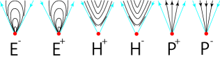
Figure 22. Two parabolic sectors $P^{-}$ and $P^{+}$, two hyperbolic sectors $H^{-}$ and $H^{+}$ with clockwise and anti-clockwise orbit directions, and two elliptic sectors $E^{+}$ and $E^{-}$ with clockwise and anti-clockwise orbit directions respectively.

A singular point $x$ is finitely sectored if either a center or there is an open neighborhood of $x$ which is an open disk and is a finite union of $\{x\}$, parabolic sectors, hyperbolic sectors, and elliptic sectors such that a pair of distinct sectors intersects at most two orbit arcs. Note that a flow with finitely sectored singular points has at most finitely many singular points. A connected component of the union of open elliptic sectors of a singular point is called a maximal open elliptic sector. Note that a maximal open elliptic sector $U$ is invariant and has the $\omega$- and $\alpha$-limit set $\{x\}$ of any point in $U$ such that the orbit closure $\overline{O(y)}=O(y)\sqcup\{x\}$ for any point $y\in U$ bounds an invariant flow box in $U$. For a finitely sectored singular point $x$, a nonempty open parabolic sector is a maximal open parabolic sector if it is an open parabolic sector contained in the complement of the union of maximal elliptic open sectors of $x$ and hyperbolic sectors of $x$ which is maximal with respect to the inclusion order. A flow is of weakly finite type if it is finitely sectored, there are at most finitely many limit cycles, and $\mathrm{LD}(v)\sqcup\mathrm{E}(v)=\emptyset$. A flow is of weakly finite-like type if the blow-down flow is of weakly finite type. A flow has sectored-like singular points if each singular point of the blow-down flow is finitely sectored. Then a flow is of weakly finite-like type if and only if it has sectored-like singular points, there are at most finitely many limit cycles, and any recurrent orbits are closed. A separatrix is a hyperbolic (resp. elliptic, parabolic) border separatrix if it is contained in the boundary of a hyperbolic sector (resp. a maximal open elliptic sector, a maximal open parabolic sector). A separatrix is a border separatrix if it is either hyperbolic, elliptic, or parabolic border separatrix. Denote by $\mathop{\partial_{\mathrm{h}(v)}}$ the boundary of the union of hyperbolic separatrices, and by $\mathop{\partial_{\mathrm{e/p}(v)}}$ the boundary of the union of non-hyperbolic elliptic/parabolic separatrices which are not hyperbolic. Similarly, a separatrix is a hyperbolic (resp. elliptic, parabolic) border-like separatrix of a flow $v$ on a surface $S$ if it is contained in the boundary of a hyperbolic sector (resp. a maximal open elliptic sector, a maximal open parabolic sector) as a subset of $S_{\mathrm{col}}$. By definition, note that $\mathop{\partial_{\mathrm{P}(v)}}\subseteq\mathop{\partial_{\mathrm{e/p}(v)}}$. Denote by $\mathop{\mathrm{Bd}}_{0+}(v)$ the union $\mathop{\mathrm{Bd}}_{0}(v)\sqcup\mathop{\partial_{\mathrm{h}(v)}}$. Note that the union of the boundaries of hyperbolic sectors contains the ss-separatrices and multi-saddle separatrices, and that if $v$ is quasi-regular then $\mathop{\mathrm{Bd}}_{0+}(v)=\mathop{\mathrm{Bd}}_{0}(v)$. Similarly, denote by $\mathop{\mathrm{BD}}_{+}(v)$ (resp. $\mathop{\mathrm{Bd}}_{+}(v)$) the union of $\mathop{\mathrm{BD}}(v)$ (resp. $\mathop{\mathrm{Bd}}(v)$), $\mathop{\mathrm{Sing}}(v)$, and border-like separatrices. Note that the union of the boundaries of hyperbolic sectors contains the ss-separatrices and multi-saddle separatrices, and that if $v$ is quasi-regular then $\mathop{\mathrm{BD}}_{+}(v)=\mathop{\mathrm{BD}}(v)$ and $\mathop{\mathrm{Bd}}_{+}(v)=\mathop{\mathrm{Bd}}(v)$. We have the following relations among border point sets and relative concepts.

Lemma 7.1.

Let $v$ be a flow with finitely sectored singular points on a compact surface. The following statements hold:
(1) $\mathop{\mathrm{Bd}}_{+}(v)-\mathop{\mathrm{Bd}}_{0+}(v)=\mathop{\partial_{\mathrm{e/p}(v)}}\cup\partial_{\mathop{\mathrm{Per}}(v)}$.
(2) $\mathop{\mathrm{BD}}_{+}(v)-\mathop{\mathrm{Bd}}_{0+}(v)=\mathop{\partial_{\mathrm{e/p}(v)}}\cup\partial_{\mathop{\mathrm{Per}}(v)}\cup\mathop{\mathrm{Per}}_{1}(v)$.
(3) If $v$ is of weakly finite type, then $\mathop{\mathrm{Bd}}_{0+}(v)=\mathop{\mathrm{Sing}}(v)\sqcup\partial^{-}\mathop{\mathrm{Per}}(v)\sqcup\mathop{\partial_{\mathrm{h}(v)}}$ is the finite union of singular points, limit cycles, and hyperbolic border separatrices.
(4) If $v$ is of weakly finite type, then $\mathop{\mathrm{BD}}_{+}(v)$ is the finite union of singular points, limit cycles, one-sided periodic orbits, and border separatrices.

Proof.

Recall that $\mathop{\mathrm{Bd}}_{0}(v)=\mathop{\mathrm{Sing}}(v)\sqcup\partial^{-}\mathop{\mathrm{Per}}(v)\sqcup\mathop{\mathrm{P}_{\mathrm{semi}}}(v)\sqcup\mathrm{E}(v)$ and $\mathop{\mathrm{BD}}(v)=\partial\mathop{\mathrm{Sing}}(v)\cup\partial\mathop{\mathrm{Per}}(v)\cup\partial_{\mathop{\mathrm{Per}}(v)}\cup\mathop{\mathrm{Per}}_{1}(v)\cup\partial\mathrm{P}(v)\cup\mathop{\mathrm{P}_{\mathrm{sep}}}(v)\cup\partial\mathrm{LD}(v)\cup\partial\mathrm{E}(v)$. By definitions, we obtain $\mathop{\mathrm{Sing}}(v)\sqcup\mathop{\mathrm{P}_{\mathrm{semi}}}(v)\subseteq\mathop{\mathrm{BD}}_{+}(v)\cap\mathop{\mathrm{Bd}}_{0+}(v)$. From $\partial^{-}\mathop{\mathrm{Per}}(v)\sqcup\mathrm{E}(v)\subseteq\mathop{\mathrm{BD}}(v)\subseteq\mathop{\mathrm{BD}}_{+}(v)$, we have $\mathop{\mathrm{Bd}}_{0+}(v)\subseteq\mathop{\mathrm{BD}}_{+}(v)$.

We claim that $\mathop{\mathrm{BD}}_{+}(v)-\mathop{\mathrm{Bd}}_{0+}(v)=\partial_{\mathop{\mathrm{Per}}(v)}\sqcup\mathop{\mathrm{Per}}_{1}(v)\sqcup\mathop{\partial_{\mathrm{e/p}(v)}}$. Indeed, by definitions, the set difference $\mathop{\mathrm{P}_{\mathrm{sep}}}(v)\setminus\mathop{\mathrm{P}_{\mathrm{semi}}}(v)=\mathop{\partial_{\mathrm{P}(v)}}\subseteq\mathop{\partial_{\mathrm{e/p}(v)}}$ consists of orbits on $\partial S$ between $\partial$-sources and $\partial$-sinks. From Lemma 3.2, Lemma 4.4, and Proposition 4.5, since $v$ is finitely sectored, the boundary $\partial\mathrm{LD}(v)=\partial^{+}\mathrm{LD}(v)$ consists of singular points and connecting separatrices between hyperbolic sectors because of the finitely sectored property. In other words, we have $\partial\mathrm{LD}(v)\subseteq\mathop{\mathrm{Sing}}(v)\sqcup\mathop{\partial_{\mathrm{h}(v)}}\subseteq\mathop{\mathrm{Bd}}_{0+}(v)$. By the finitely sectored property, Lemma 3.2 and Proposition 4.5 imply that $\partial^{+}\mathop{\mathrm{Per}}(v)\subseteq\mathop{\mathrm{Sing}}(v)\sqcup\mathop{\partial_{\mathrm{h}(v)}}\subseteq\mathop{\mathrm{Bd}}_{0+}(v)$. From Lemma 3.2 and Lemma 4.4, the openness of $\mathrm{LD}(v)$ implies that $\partial^{+}\mathrm{P}(v)\subseteq\partial^{-}\mathop{\mathrm{Sing}}(v)\sqcup\partial^{-}\mathop{\mathrm{Per}}(v)\sqcup\mathrm{E}(v)\subseteq\mathop{\mathrm{Bd}}_{0}(v)$. By the finitely sectored property, the union $\mathop{\mathrm{P}_{\mathrm{semi}}}(v)$ consists of semi-saddle separatrices contained in the boundaries of hyperbolic sectors and so $\mathop{\mathrm{P}_{\mathrm{semi}}}(v)\subseteq\mathop{\partial_{\mathrm{h}(v)}}$. Proposition 4.10 implies that $\partial^{-}\mathrm{P}(v)=(\partial^{+}\mathop{\mathrm{Per}}(v)\cup\partial^{+}\mathrm{LD}(v)\cup\partial^{+}\mathrm{E}(v))\setminus\mathop{\mathrm{Sing}}(v)\subseteq\mathop{\partial_{\mathrm{h}(v)}}\subseteq\mathop{\mathrm{Bd}}_{0+}(v)$. The claim is completed.

This completes the assertion (1). Since $\mathop{\mathrm{BD}}(v)=\mathop{\mathrm{Bd}}(v)\sqcup\mathop{\mathrm{Per}}_{1}(v)$, we have that $\mathop{\mathrm{Bd}}_{+}(v)-\mathop{\mathrm{Bd}}_{0+}(v)=\mathop{\partial_{\mathrm{e/p}(v)}}\cup\partial_{\mathop{\mathrm{Per}}(v)}$. Therefore the assertion (2) holds.

Suppose that $v$ is of weakly finite type. By Lemma 3.4, the finite existence of limit cycles implies that $\partial^{-}\mathop{\mathrm{Per}}(v)$ consists of finitely many limit cycles. The non-existence of non-closed recurrent points implies that $\mathop{\mathrm{Bd}}_{0}(v)=\mathop{\mathrm{Sing}}(v)\sqcup\partial^{-}\mathop{\mathrm{Per}}(v)\sqcup\mathop{\mathrm{P}_{\mathrm{semi}}}(v)$. Since $\mathop{\mathrm{P}_{\mathrm{semi}}}(v)\subseteq\mathop{\partial_{\mathrm{h}(v)}}$, we obtain that $\mathop{\mathrm{Bd}}_{0+}(v)=\mathop{\mathrm{Sing}}(v)\sqcup\partial^{-}\mathop{\mathrm{Per}}(v)\sqcup\mathop{\partial_{\mathrm{h}(v)}}$ is the finite union of singular points, limit cycles, hyperbolic border separatrices. Therefore the assertion (3) holds. Since $\mathop{\partial_{\mathrm{P}(v)}}$ consists of separatrices which are non-hyperbolic but elliptic/parabolic separatrices and the union $\partial_{\mathop{\mathrm{Per}}(v)}\sqcup\mathop{\mathrm{Per}}_{1}(v)$ is the union of one-sided orbits, the assertion (4) holds. ∎

7.2. Blow-up of quasi-regular flows into flows with sectored-like singular points

We can deform any flow with sectored singular points on a compact surface into a quasi-regular flow by finitely many operations which increase at most finitely many non-recurrent orbits but preserves both $\mathop{\mathrm{Bd}}_{0+}$ and $\mathop{\mathrm{BD}}_{+}$.

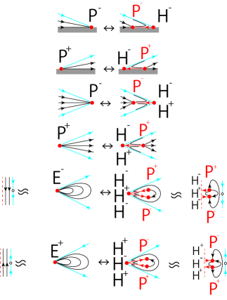
Figure 23. Two deformations of parabolic sectors on the boundary into a hyperbolic sector and a $\partial$-sink/$\partial$-source, two deformations of parabolic sectors outside of the boundary into two hyperbolic sectors, a sink/source, and a separatrix connecting singular points, and two deformations of maximal elliptic sectors into a hyperbolic sectors, a source, a parabolic sector, and a separatrix connecting singular points

We call that deformations at two on the top (resp. middle, bottom) in Figure 23 are blow-up operations of parabolic sectors on the boundary (resp. parabolic sectors outside of the boundary, maximal elliptic sectors). The tuple is called a lift of the finitely sectored singular point with parabolic sectors on the boundary (resp. parabolic sectors outside of the boundary, maximal elliptic sectors). Note that each blow-up operation of a parabolic sector (resp. maximal elliptic sector) replaces a singular point $x$ into a tuple of a singular point with hyperbolic sectors, a ($\partial$-)sink/($\partial$-)source, and a separatrix between them (resp. a singular point with hyperbolic sectors, a sink, a source, and two separatrices between them) as in Figure 23. In fact, for a singular point $x$ with parabolic (resp. maximal elliptic) sectors, collapsing a lift of the finitely sectored singular point $x$, we have a surjection $p:S\to S$ such that the restriction $p|_{S-p^{-1}(x)}:S-p^{-1}(x)\to S-\{x\}$ to the complement of the inverse image of $x$ is identical and that $p^{-1}(x)$ is a tuple of a singular point with hyperbolic sectors, a ($\partial$-)sink/($\partial$-)source, and a separatrix between them (resp. a tuple of a sink, a source, a singular point with hyperbolic sectors, a hyperbolic border separatrix from the sink, and a hyperbolic separatrix to the source). Then the surjection $p$ is called a blow-up mapping to the finitely sectored singular point $x$. By construction, we have the following observation.

Lemma 7.2.

For any blow-up mapping $p:S\to S$ to a finitely sectored singular point $x$, we have following relations:
$(1)$ $(S-p^{-1}(x))/v_{p}=(S-\{x\})/v$ as quotient spaces, where $v_{p}$ is the lift of $v$.
$(2)$ $(S/v_{p})/\sim_{x}$ is canonically homeomorphic to $S/v$, where $\sim_{x}$ is an equivalence relation defined as follows: for any point $y,z$, define $y\sim_{x}z$ if either $O(y)=O(z)$ or $y,z\in p^{-1}(x)$.

A blow-up operation of an elliptic sectored singular point $x$ to a maximal elliptic disk preserves the border point set except $x$ and its lift.

Lemma 7.3.

Let $x$ be a finitely sectored singular point and $p:S\to S$ the lift of the finitely sectored singular point with elliptic sectors. Then $\mathop{\mathrm{BD}}_{+}(v)-\{x\}=\mathop{\mathrm{BD}}_{+}(v_{p})-p^{-1}(x)$.

A blow-up operation of a parabolic sectored singular point $x$ to a maximal parabolic sector preserves the border point set except $x$ and its lift.

Lemma 7.4.

Let $x$ be a finitely sectored singular point with parabolic sector and $p:S\to S$ the lift of the finitely sectored singular point with parabolic sectors. Then $\mathop{\mathrm{BD}}_{+}(v)-\{x\}=\mathop{\mathrm{BD}}_{+}(v_{p})-p^{-1}(x)$.

Taking finitely many lifts of finitely sectored singular points, we have the following blow-up operation.

Lemma 7.5.

For any flow $v$ with finitely sectored singular points on a compact surface $S$, applying finitely many blow-up operations of maximal elliptic sectors as possible, and applying finitely many blow-up operations of parabolic sectors as possible, the following statements hold for the resulting flow $w$:
(1) The resulting flow $w$ is a quasi-regular flow on $S$.
(2) The orbit space for $w$ restricted to the complement of the union of lifts of finitely sectored singular points is equal to the orbit space for $v$ restricted to the complement of finitely sectored singular points.
(3) The union of lifts of finitely sectored singular points is contained in $\mathop{\mathrm{BD}}_{+}(w)$.
(4) $v|_{S-\mathop{\mathrm{BD}}(v)}=w|_{S-\mathop{\mathrm{BD}}_{+}(w)}$.

7.3. Decompositions of flows with sectored-like singular points

For a point $z\in S_{\mathrm{col}}$, denote by $\alpha_{v_{\mathrm{col}}}(z)\subseteq S_{\mathrm{col}}$ (resp. $\omega_{v_{\mathrm{col}}}(z)\subseteq S_{\mathrm{col}}$) the $\alpha$-limit (resp. $\omega$-limit) set of a point $z$ with respect to $v_{\mathrm{col}}$. By Theorem 5.3 and Corollary 5.4, the blow-up operations imply the following main results.

Theorem 7.6.

Each connected component of $S-\mathop{\mathrm{Bd}}_{0+}(v)$ for a flow $v$ with sectored-like singular points on a compact surface $S$ is one of the following invariant open subsets exclusively:
$(1)$ A flow box in $\mathrm{P}(v)$, whose orbit space is an interval,
$(2)$ An annulus in $\mathrm{P}(v)$, whose orbit space is a circle,
$(3)$ A torus in $\mathop{\mathrm{Per}}(v)$, whose orbit space is a circle,
$(4)$ A Klein bottle in $\mathop{\mathrm{Per}}(v)$, whose orbit space is an interval,
$(5)$ An annulus in $\mathop{\mathrm{Per}}(v)$, whose orbit space is an interval,
$(6)$ A Möbius band in $\mathop{\mathrm{Per}}(v)$, whose orbit space is an interval, or
$(7)$ An essential subset in $\mathrm{LD}(v)$, whose orbit class space is a singleton.

Moreover, the following statements hold:
$(a)$ For any connected component $U$ in $\mathrm{P}(v_{\mathrm{col}})\setminus\mathop{\mathrm{Bd}}_{+}(v_{\mathrm{col}})=\mathrm{P}(v)\setminus\mathop{\mathrm{Bd}}_{0+}(v)$ and for any points $x,y\in U$, we have $\alpha_{v_{\mathrm{col}}}(x)=\alpha_{v_{\mathrm{col}}}(y)$ and $\omega_{v_{\mathrm{col}}}(x)=\omega_{v_{\mathrm{col}}}(y)$.
$(b)$ For any connected component $U$ in $\mathrm{LD}(v)$ and for any points $x,y\in U$, we have $\overline{O(x)}=\overline{O(y)}=\overline{U}\subseteq S$.
$(c)$ Each of the vertical $\alpha$- and $\omega$-vertical boundaries of any connected components of $S-\mathop{\mathrm{Bd}}_{0+}(v_{\mathrm{col}})$ in the case $(1)$ and $(2)$ is a finite union of closed orbits and separatrices as a subset of $S_{\mathrm{col}}$ unless the vertical boundary intersects $\mathrm{E}(v_{\mathrm{col}})=\mathrm{E}(v)$.
$(d)$ Each of the left and right transverse boundaries of any connected components of $S-\mathop{\mathrm{Bd}}_{0+}(v_{\mathrm{col}})$ in the case $(1)$ and $(4)$ is an immersed line which is a finite union of closed orbits and separatrices as a subset of $S_{\mathrm{col}}$ unless the left/right transverse boundary intersects $\mathrm{E}(v_{\mathrm{col}})=\mathrm{E}(v)$.

Theorem 7.7.

Each connected component of $S-\mathop{\mathrm{BD}}_{+}(v)$ for a flow $v$ with sectored-like singular points on a compact surface $S$ is one of the following invariant open subsets exclusively:
$(1)$ A flow box in $\mathrm{P}(v)$, whose orbit space is an interval,
$(2)$ An annulus in $\mathrm{P}(v)$, whose orbit space is a circle,
$(3)$ A torus in $\mathop{\mathrm{Per}}(v)$, whose orbit space is a circle,
$(4)$ An annulus in $\mathop{\mathrm{Per}}(v)$, whose orbit space is an interval, or
$(5)$ An essential subset in $\mathrm{LD}(v)$, whose orbit class space is a singleton.

Moreover, the following statements hold:
$(a)$ For any connected component $U$ in $\mathrm{P}(v_{\mathrm{col}})\setminus\mathop{\mathrm{Bd}}_{+}(v_{\mathrm{col}})=\mathrm{P}(v)\setminus\mathop{\mathrm{BD}}_{+}(v)$ and for any points $x,y\in U$, we have $\alpha_{v_{\mathrm{col}}}(x)=\alpha_{v_{\mathrm{col}}}(y)$ and $\omega_{v_{\mathrm{col}}}(x)=\omega_{v_{\mathrm{col}}}(y)$.
$(b)$ For any connected component $U$ in $\mathrm{LD}(v)$ and for any points $x,y\in U$, we have $\overline{O(x)}=\overline{O(y)}=\overline{U}\subseteq S$.
$(c)$ Each of the vertical $\alpha$- and $\omega$-vertical boundaries of any connected components of $S_{\mathrm{col}}-\mathop{\mathrm{BD}}_{+}(v_{\mathrm{col}})$ in the case $(1)$ and $(2)$ is a finite union of closed orbits and separatrices as a subset of $S_{\mathrm{col}}$ unless the vertical boundary intersects $\mathrm{E}(v_{\mathrm{col}})=\mathrm{E}(v)$.
$(d)$ Each of the left and right transverse boundaries of any connected components of $S_{\mathrm{col}}-\mathop{\mathrm{BD}}_{+}(v_{\mathrm{col}})$ in the case $(1)$ and $(4)$ is an immersed line which is a finite union of closed orbits and separatrices as a subset of $S_{\mathrm{col}}$ unless the left/right transverse boundary intersects $\mathrm{E}(v_{\mathrm{col}})=\mathrm{E}(v)$.

Lemma 7.1 and the previous theorem imply the following description of flows of weakly finite-like type.

Corollary 7.8.

Each connected component of $S-\mathop{\mathrm{BD}}_{+}(v)$ for a flow $v$ of weakly finite-like type on a compact surface $S$ is one of the following invariant open subsets exclusively:
$(1)$ A flow box in $\mathrm{P}(v)$, whose orbit space is an interval,
$(2)$ An annulus in $\mathrm{P}(v)$, whose orbit space is a circle,
$(3)$ A torus in $\mathop{\mathrm{Per}}(v)$, whose orbit space is a circle, or
$(4)$ An annulus in $\mathop{\mathrm{Per}}(v)$, whose orbit space is an interval.

Moreover, the union $\mathop{\mathrm{BD}}_{+}(v_{\mathrm{col}})$ is the finite union of singular points, limit cycles, one-sided periodic orbits, and border separatrices of $v_{\mathrm{col}}$.

Theorem 6.3, Lemma 7.5, and the previous corollary imply the following statement.

Theorem 7.9.

The set of flows of weakly finite type on compact surfaces is enumerable.

8. Graphs of surface flows

We construct a complete invariant of a flow of finite type as a finite labelled graph.

8.1. Abstract multi-graphs of separatrices and one-sided orbits

Proposition 4.17 and Proposition 6.2 imply the following statement.

Corollary 8.1.

The following statements hold for a flow $v$ of finite type on a compact surface $S$:
$(1)$ The quotient spaces $D_{\mathrm{ss}}(v)/{v}_{\mathrm{ex}}$, $\mathop{\mathrm{Bd}}(v)/{v}_{\mathrm{ex}}$, and $\mathop{\mathrm{BD}}(v)/{v}_{\mathrm{ex}}$ are finite abstract multi-graphs.
$(2)$ The complement $(S-D_{\mathrm{ss}}(v))/v$ $(\mathrm{resp.}$ $(S-\mathop{\mathrm{Bd}}(v))/v$, $S-\mathop{\mathrm{BD}}(v)/v)$ is a finite disjoint union of intervals and circles such that the boundary of a connected component of $S-D_{\mathrm{ss}}(v)$ $(\mathrm{resp.}$ $S-\mathop{\mathrm{Bd}}(v)$, $S-\mathop{\mathrm{BD}}(v))$ consists of finitely many closed orbits and finitely many separatrices.

Each connected component of the complement $S-D_{\mathrm{ss}}(v)$ (resp. $S-\mathop{\mathrm{Bd}}(v)$, $S-\mathop{\mathrm{BD}}(v)$) of a flow $v$ of finite type on a compact surface $S$ is called a canonical domain of it. We call that an invariant flow box (resp. invariant periodic annulus, invariant transverse annulus) is a canonical region if it is maximal such domain with respect to the inclusion relation. Note that definition of a canonical region of $v$ for the orbit complex [22, 26, 27] is slightly different from our definitions, and that a canonical domain which is not a periodic torus for a flow of finite type on a compact surface corresponds to a canonical region.

8.2. Dual graphs of the border point set $\mathop{\mathrm{BD}}(v)$

For a flow $v$ of finite type on a compact surface $S$, define the dual graph $G^{\mathrm{BD}(v)}=(V^{\mathop{\mathrm{BD}}(v)},E^{\mathop{\mathrm{BD}}(v)})$ of the border point set $\mathop{\mathrm{BD}}(v)$ as follows: The vertex set $V^{\mathop{\mathrm{BD}}(v)}$ consists of periodic tori and canonical domains of $\mathop{\mathrm{BD}}(v)$ (i.e. the connected components of $S-\mathop{\mathrm{BD}}(v)$) each of which is either an invariant flow box, an invariant transverse annulus, or an invariant periodic annulus. An edge $U_{i}U_{j}$ exists if and only if $\dim(\overline{U_{i}}\cap\overline{U_{j}})=1$. We equip any canonical domain with a local orientation which is a mapping $\mathcal{O}:V^{\mathop{\mathrm{BD}}(v)}\to\{-,+\}$.

8.3. Labels of $V^{\mathop{\mathrm{BD}}(v)}$

For a quasi-regular flow $v$ on a compact surface, define a label $l^{\mathop{\mathrm{BD}}(v)}:V^{\mathop{\mathrm{BD}}(v)}\to\{\mathbb{D},\widetilde{\mathbb{A}},\mathbb{A},\mathbb{T},\mathbb{L}\}$ as follows: the label $l^{\mathop{\mathrm{BD}}(v)}(U)$ is defined as follows:
$l^{\mathop{\mathrm{BD}}(v)}(U):=\mathbb{D}$ if $U$ is an invariant open flow box in $\mathrm{P}(v)$,
$l^{\mathop{\mathrm{BD}}(v)}(U):=\widetilde{\mathbb{A}}$ if $U$ is an open transverse annulus in $\mathrm{P}(v)$,
$l^{\mathop{\mathrm{BD}}(v)}(U):=\mathbb{A}$ if $U$ is an open annulus in $\mathop{\mathrm{Per}}(v)$,
$l^{\mathop{\mathrm{BD}}(v)}(U):=\mathbb{T}$ if $U$ is a torus in $\mathop{\mathrm{Per}}(v)$,
$l^{\mathop{\mathrm{BD}}(v)}(U):=\mathbb{L}$ if $U$ is an essential open subset in $\mathrm{LD}(v)$.
By Corollary 5.4, the label $l^{\mathop{\mathrm{BD}}(v)}$ is well-defined. Set $\Sigma_{\mathrm{Top}}^{1}:=\{\mathbb{D},\widetilde{\mathbb{A}},\mathbb{A},\mathbb{T},\mathbb{L}\}$.

8.3.1. Labels for transverse and vertical boundary information

Recall that, for an invariant open subset $A$, define the vertical boundary $\partial_{\perp}A$ of $A$ as follows: $\partial_{\perp}^{\alpha}A:=(\bigcup_{x\in A}\alpha(x))\setminus A$, $\partial_{\perp}^{\omega}A:=(\bigcup_{x\in A}\omega(x))\setminus A$, and $\partial_{\perp}A:=\partial_{\perp}^{\alpha}A\cup\partial_{\perp}^{\omega}A$. Define a label $\partial_{\perp}^{\bullet}=(\partial_{\perp}^{\alpha}/\hat{v},\partial_{\perp}^{\omega}/\hat{v}):V^{\mathop{\mathrm{BD}}(v)}\to 2^{\mathrm{BD}(v)/\hat{v}}\times 2^{\mathrm{BD}(v)/\hat{v}}$ by

$$\partial_{\perp}^{\bullet}(U)=(\partial_{\perp}^{\alpha}(U)/\hat{v},\partial_{\perp}^{\omega}(U)/\hat{v}):=(\alpha(x)/\hat{v},\omega(x)/\hat{v})$$

for any $U\in V^{\mathop{\mathrm{BD}}(v)}$ and for some $x\in U$. By Corollary 5.4, the $\omega$-limit and $\alpha$-limit sets of any point in $U$ are so of $x$ and thus the label $l^{\mathop{\mathrm{BD}}(v)}$ is well-defined. Note that the label $\partial_{\perp}$ can be considered as the restriction of the pair $(\leq_{\hat{\alpha}},\leq_{\hat{\omega}})$ on $S/\hat{v}$.

Define a label $\partial_{\pitchfork}^{\bullet}:=(\partial_{\pitchfork}^{R}/\hat{v},\partial_{\pitchfork}^{L}/\hat{v}):V^{\mathop{\mathrm{BD}}(v)}\to 2^{\mathrm{BD}(v)/\hat{v}}\times 2^{\mathrm{BD}(v)/\hat{v}}$ by

$$\partial_{\pitchfork}^{\bullet}(U):=(\partial_{\pitchfork}^{R}(U)/\hat{v},\partial_{\pitchfork}^{L}(U)/\hat{v}))$$

for any $U\in V^{\mathop{\mathrm{BD}}(v)}$.

8.3.2. A spiral direction for a region whose $\omega$-limit (resp. $\alpha$-limit) set is a circuit

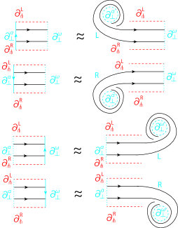
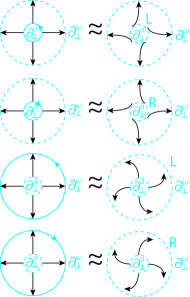
Figure 24. Schematic pictures and their spiral structures of invariant flow boxes and transverse annuli

Let $\gamma$ be a non-trivial circuit and $U$ either an oriented invariant flow box or an oriented transverse annulus each of whose $\omega$-limit set is $\gamma$. The spiral direction $\mathcal{D}_{\partial_{\perp}^{\alpha}}(U)$ is $L$ (resp. $R$) if $U$ rotates anti-clockwise (resp. clockwise) around a non-trivial circuit as the upper part of Figure 24. The spiral direction $\mathcal{D}_{\partial_{\perp}^{\omega}}(U)$ is $L$ (resp. $R$) if $U$ rotates anti-clockwise (resp. clockwise) around a non-trivial circuit as the lower part of Figure 24. Otherwise the spiral direction $\mathcal{D}_{\partial_{\perp}^{\sigma}}(U)$ is defined as $0$. Note that the direction with respect to the local orientation on the box or annulus is well-defined even if the limit circuit $\gamma$ is contained in a non-orientable compact surface.

For a flow $v$ of finite type on a compact surface, define a label $\mathcal{D}_{\partial_{\perp}}=(\mathcal{D}_{\partial_{\perp}^{\alpha}},\mathcal{D}_{\partial_{\perp}^{\omega}}):V^{\mathop{\mathrm{BD}}(v)}\to\{R,L,0\}\times\{R,L,0\}$ by

$$\mathcal{D}_{\partial_{\perp}}(U):=(\mathcal{D}_{\partial_{\perp}^{\alpha}}(U),\mathcal{D}_{\partial_{\perp}^{\omega}}(U))$$

for any $U\in V^{\mathop{\mathrm{BD}}(v)}$.

8.4. Graph structure of the border point set $\mathop{\mathrm{BD}}(v)$

Let $v$ be a flow of finite type on a compact surface. From Proposition 6.2, denote by $G_{\mathrm{BD}(v)}=(V_{\mathrm{BD}(v)},E_{\mathrm{BD}(v)})$ the abstract multi-graph $\mathop{\mathrm{BD}}(v)/\hat{v}_{\mathrm{ex}}$. Note that each of $V_{\mathrm{BD}(v)}$ and $E_{\mathrm{BD}(v)}$ is a subset of $G_{\mathrm{BD}(v)}=\mathop{\mathrm{BD}}(v)/\hat{v}_{\mathrm{ex}}$. Precisely, the vertex set $V_{\mathrm{BD}(v)}$ consists of multi-saddle connections, limit cycles, non-limits one-sided cycles, sinks, $\partial$-sinks, sources, $\partial$-sources, and centers. The edge set $E_{\mathrm{BD}(v)}$ consists of

(i) orbits in $\mathop{\partial_{\mathrm{P}(v)}}$,
(ii) ss-separatrices which are arranged in cyclic ways around limit circuits, sinks, and sources, and
(iii) ss-separatrices which are arranged in linear ways around $\partial$-sinks and $\partial$-sources.
Define a label $l_{\mathop{\mathrm{BD}}(v)}:V_{\mathop{\mathrm{BD}}(v)}\to\{0,1_{\partial},1_{\mathrm{non}},1_{\mathrm{lc}}\}$ as follows:
$l_{\mathop{\mathrm{BD}}(v)}(\sigma):=0$ if $\sigma\in\mathop{\mathrm{Sing}}(v)$ is either a sink, a $\partial$-sink, a source, a $\partial$-source, or a center,
$l_{\mathop{\mathrm{BD}}(v)}(\gamma):=1_{\partial}$ if $\gamma$ is a periodic orbit in $\partial S$,
$l_{\mathop{\mathrm{BD}}(v)}(\gamma):=1_{\mathrm{non}}$ if $\gamma$ is a one-sided periodic orbit outside of $\partial S$,
$l_{\mathop{\mathrm{BD}}(v)}(\gamma):=1_{\mathrm{two}}$ if $\gamma$ is a two-sided periodic orbit.
$l_{\mathop{\mathrm{BD}}(v)}(\gamma):=1_{\mathrm{ms}}$ if $\gamma$ is a multi-saddle connection diagram.
Set $\Sigma_{\mathrm{Top}}^{0}:=\{0,1_{\partial},1_{\mathrm{non}},1_{\mathrm{two}},1_{\mathrm{ms}}\}$. Note that each multi-saddle circuit with an associated collar has either semi-repelling, semi-attracting, or identical one-sided holonomy and so that a one-sided multi-saddle circuit has one of these three kinds of holonomies and a two-sided cycle has one of six kinds of holonomies.

8.5. Label of the orbit space $D(v)/v$ of the multi-saddle connection diagram

For a quasi-regular flow $v$ on a compact surface, denote by $G_{D(v)}$ the abstract multi-graph $D(v)/v$ and a label $l_{D}:G_{D(v)}\to V_{\mathop{\mathrm{BD}}(v)}$ is defined as the natural projection $D(v)/v\to D(v)/v_{\mathrm{ex}}$.

8.6. A path order on a path on the transverse boundary of an invariant flow box

Let $\mu_{R}:=(0,1)\times\{0\}$ be an open interval, $\mathbb{D}:=(0,1)\times(0,1)$ a canonical invariant flow box whose orbits are of form $(0,1)\times\{t\}$, $U$ an oriented open flow box, and $h_{R}:(0,1)\times[0,1)=\mathbb{D}\sqcup\mu_{R}\to U\sqcup\partial_{\pitchfork}^{R}U$ a mapping such that the restriction $h_{R}|_{\mathbb{D}}:\mathbb{D}\to U$ is an orientation-preserving topological conjugacy and the restriction $h_{R}|_{\mu_{R}}:\mu_{R}\to\partial_{\pitchfork}^{R}U$ is an immersion except singular points. Since an immersion except singular points lifts orbits into the domain, the interval $\mu_{R}$ can be considered as the union of orbits. Note that the restriction $h_{R}|_{\mu_{R}}$ need not be injective. Suppose that the interval $\mu_{R}$ consists of finitely many orbits. Define an equivalence relation $\sim_{\partial_{\pitchfork}^{R}U}$ on $\mu_{R}$ as follows: $x\sim y$ if there is a connected component $J$ of $h_{R}^{-1}(O)$ for some orbit $O$ in $\partial_{\pitchfork}^{R}U$ such that $J$ contains $x$ and $y$. Then $\mu_{R}/\sim_{\partial_{\pitchfork}^{R}U}$ is a finite set with the total order $(J_{1},J_{2},\ldots,J_{n})$ (i.e. $J_{1}<J_{2}<\cdots<J_{n}$) induced by the interval $\mu_{R}$ such that either $\omega(J_{i})=J_{i+1}$ or $J_{i}=\alpha(J_{i+1})$ for any $i\in\{1,\ldots,n-1\}$. We call a sequence $(h_{R}(J_{1}),h_{R}(J_{2}),\ldots,h_{R}(J_{n}))$ of orbits in $\partial_{\pitchfork}^{R}U$ a path order of $\partial_{\pitchfork}^{R}U$ and denoted by $\leq_{\partial_{\pitchfork}^{R}}(U)$ (or $\leq_{\partial_{\pitchfork}^{R}}$ with respect to $U$) (i.e. $h_{R}(J_{1})\leq_{\partial_{\pitchfork}^{R}}h_{R}(J_{2})\leq_{\partial_{\pitchfork}^{R}}\cdots\leq_{\partial_{\pitchfork}^{R}}h_{R}(J_{n})$ with respect to $U$). Note that path orders need not be total orders because $h_{R}|_{\mu_{R}}$ is not injective in general. Notice that we can define a path order unless the assumption that $\mu_{R}$ consists of finitely many orbits in a similar way. Similarly, we define a path order $\leq_{\partial_{\pitchfork}^{L}}(U)$ of the left transverse boundary $\partial_{\pitchfork}^{L}U$.

8.7. A cyclic order

Define a cyclic relation $\sim_{c}$ on a finite set $F$ with $n$ points as follows: $(O_{1},O_{2},\ldots,O_{n})\sim_{c}(O_{i_{1}},O_{i_{2}},\ldots,O_{i_{n}})$ if $F=\{O_{1},O_{2},\ldots,O_{n}\}$ and there is an integer $k=0,1,\ldots,n-1$ such that $j-i_{j}\equiv k\mod n$ for any $j=1,\ldots,n$. An equivalence class is called a cyclic class of $F$ and denoted by $[O_{1},O_{2},\ldots,O_{n}]$. Note that a cyclic class of a $n$-point sets corresponds to a $n$-point subset of an oriented circle.

8.8. A circuit order on multi-saddle circuits

Each ($\partial$-)sink (resp. ($\partial$-)source) $x$ with a basin $\mathbb{A}$ has the trivial order on the singular point, called a trivial circuit order and denoted by $\leq_{\mathbb{A}}(x)$. Each center $x$ with a periodic annulus $U$ has the trivial order on the singular point, called a trivial circuit order and denoted by $\leq_{U}(x)$.

Let $\gamma$ be a multi-saddle circuit with a collar $\mathbb{A}=\mathbb{S}^{1}\times(0,1)$ and an associated immersion $h|_{\mathbb{S}^{1}\times\{0\}}:\mathbb{S}^{1}\times\{0\}\to\gamma$ except singular points. Then the composition $p_{\partial}:=h\circ p^{-1}:\mathbb{S}^{1}\to\gamma$ is an immersion except singular points, called a multi-saddle circuit with the spiral direction for $\mathbb{A}$, where $p:\mathbb{S}^{1}\times\{0\}\to\mathbb{S}^{1}$ is the canonical projection. Since an immersion except singular points lifts orbits into the domain, the circle $\mathbb{S}^{1}\times\{0\}$ can be considered as the union of orbits. Suppose that the circuit $\gamma$ consists of finitely many orbits. Define an equivalence relation $\sim_{\mathbb{A}}$ on $\mathbb{S}^{1}$ as follows: $x\sim_{\mathbb{A}}y$ if there is a connected component $I$ of $p_{\partial}^{-1}(O)$ for some orbit $O$ in $\gamma$ such that $I$ contains $x$ and $y$. Then $\mathbb{S}^{1}/\sim_{\mathbb{A}}$ is a finite set with the induced cyclic order $[J_{1},J_{2},\ldots,J_{n}]$ by the circle $\mathbb{S}^{1}$ such that either $\omega(J_{i})=J_{i+1}$ or $J_{i}=\alpha(J_{i+1})$ for any $i\in\{0,\ldots,n-1\}$, where $J_{0}:=J_{n}$.

Consider a sequence $(p_{\partial}(J_{1}),p_{\partial}(J_{2}),\ldots,p_{\partial}(J_{n}))$ of orbits in $\gamma$ and define an equivalence relation $\approx_{\mathbb{A}}$ as follows:

$$(p_{\partial}(J_{1}),p_{\partial}(J_{2}),\ldots,p_{\partial}(J_{n}))\approx_{\mathbb{A}}(p_{\partial}(J_{i_{1}}),p_{\partial}(J_{i_{2}}),\ldots,p_{\partial}(J_{i_{n}}))$$

if there is an integer $k=0,1,\ldots,n-1$ such that $j+k=i_{j}$ for any $j=1,\ldots,n$, where $J_{n+l}:=J_{l}$ for $l=0,\ldots,n-1$. We call an equivalence class a circuit order of $\gamma$ and denoted by $\leq_{\mathbb{A}}(\gamma)$. Note that a circuit class is a quotient space of a cyclic order. If the circuit $\gamma$ is semi-repelling (resp. semi-attracting) on a basin $\mathbb{A}$, then a circuit order $\leq_{\mathbb{A}}(\gamma)$ is denoted by $\leq_{\partial_{\perp}^{\alpha}}(\mathbb{A})$ (resp. $\leq_{\partial_{\perp}^{\omega}}(\mathbb{A})$).

Moreover, if a canonical region $U$ intersect the semi-repelling (reps. semi-attracting) basin $\mathbb{A}$, then we also write $\leq_{\partial_{\perp}^{\alpha}}(U):=\leq_{\partial_{\perp}^{\alpha}}(\mathbb{A})$ (resp. $\leq_{\partial_{\perp}^{\omega}}(U):=\leq_{\partial_{\perp}^{\omega}}(\mathbb{A})$). If the circuit $\gamma$ is the right (resp. left) transverse boundary of a periodic annulus $U$, then a circuit order $\leq_{U}(\gamma)$ is denoted by $\leq_{\partial_{\pitchfork}^{R}}(U)$ (resp. $\leq_{\partial_{\pitchfork}^{L}}(U)$). Notice that we can define a circuit order unless the assumption that $\gamma$ consists of finitely many orbits in a similar way.

8.9. Reversion of a local orientation of a canonical domain

Let $v$ be a flow of finite type on a compact surface $S$. A local orientation reversion ${V}^{\mathrm{Rev}}:V_{\mathrm{BD}(v)}\to V_{\mathrm{BD}(v)}$ of canonical domains is an identity as a set with $\mathcal{O}^{{\mathrm{Rev}}}(U)=-\mathcal{O}(U)$, where $\mathcal{O}^{{\mathrm{Rev}}}:=\mathcal{O}\circ V^{{\mathrm{Rev}}}$. Define $\mathcal{D}_{\partial_{\perp}^{\alpha}}^{\mathrm{Rev}}(U)=L$ (resp. $R$) if $\mathcal{D}_{\partial_{\perp}^{\alpha}}(U)=R$ (resp. L). Similarly, define $\mathcal{D}_{\partial_{\perp}^{\omega}}^{\mathrm{Rev}}(U)=L$ (resp. $R$) if $\mathcal{D}_{\partial_{\perp}^{\omega}}(U)=R$ (resp. L) and

$$\mathcal{D}_{\partial_{\perp}}^{\mathrm{Rev}}:=(\mathcal{D}_{\partial_{\perp}^{\alpha}}^{\mathrm{Rev}},\mathcal{D}_{\partial_{\perp}^{\omega}}^{\mathrm{Rev}})$$

Define $\mathcal{D}_{\partial_{\perp}^{\sigma}}^{\mathrm{Rev}}(U)=0$ if $\mathcal{D}_{\partial_{\perp}^{\sigma}}(U)=0$. Define a label

$$L^{\mathrm{BD}(v)}:V^{\mathrm{BD}(v)}\to\{\pm\}\times\Sigma_{\mathrm{Top}}^{1}\times(2^{\mathrm{BD}(v)/\hat{v}})^{4}\times\mathcal{O}_{\mathrm{circuit,path}}^{4}\times\{R,L,0\}^{2}$$

by

$$L^{\mathrm{BD}(v)}:=(\mathcal{O},l^{\mathop{\mathrm{BD}}(v)},\partial^{\mathrm{BD}(v)},\leq^{\mathrm{BD}(v)},\mathcal{D}_{\partial_{\perp}})$$

where $\mathcal{O}_{\mathrm{circuit,path}}$ is the set of finite circuit orders and path orders,

$$\partial^{\mathrm{BD}(v)}:=(\partial_{\pitchfork}^{\bullet},\partial_{\perp}^{\bullet})=(\partial_{\pitchfork}^{R}/\hat{v},\partial_{\pitchfork}^{L}/\hat{v},\partial_{\perp}^{\alpha}/\hat{v},\partial_{\perp}^{\omega}/\hat{v}):V^{\mathrm{BD}(v)}\to(2^{\mathrm{BD}(v)/\hat{v}})^{4}$$

$$\leq^{\mathrm{BD}(v)}:=(\leq_{\partial_{\pitchfork}^{R}},\leq_{\partial_{\pitchfork}^{L}},\leq_{\partial_{\perp}^{\alpha}},\leq_{\partial_{\perp}^{\omega}}):V^{\mathrm{BD}(v)}\to\mathcal{O}_{\mathrm{circuit,path}}^{4}$$

are mappings. By definition, we have

$$L^{\mathrm{BD}(v)}=(\mathcal{O},l^{\mathop{\mathrm{BD}}(v)},\partial_{\pitchfork}^{R}/\hat{v},\partial_{\pitchfork}^{L}/\hat{v},\partial_{\perp}^{\alpha}/\hat{v},\partial_{\perp}^{\omega}/\hat{v},\leq_{\partial_{\pitchfork}^{R}},\leq_{\partial_{\pitchfork}^{L}},\leq_{\partial_{\perp}^{\alpha}},\leq_{\partial_{\perp}^{\omega}},\mathcal{D}_{\partial_{\perp}^{\alpha}},\mathcal{D}_{\partial_{\perp}^{\omega}})$$

The revisions of labels are defined as follows:

$$\begin{split}L^{\mathrm{BD}(v)\mathrm{Rev}}&:=(\mathcal{O}^{{\mathrm{Rev}}},l^{\mathop{\mathrm{BD}}(v){\mathrm{Rev}}},\partial^{\mathrm{BD}(v){\mathrm{Rev}}},\leq^{\mathrm{BD}(v){\mathrm{Rev}}},\mathcal{D}_{\partial_{\perp}}^{{\mathrm{Rev}}})\\ &\,\,=(-\mathcal{O},l^{\mathop{\mathrm{BD}}(v)},\partial_{\pitchfork}^{L}/\hat{v},\partial_{\pitchfork}^{R}/\hat{v},\partial_{\perp}^{\bullet},\leq_{\partial_{\pitchfork}^{L}},\leq_{\partial_{\pitchfork}^{R}},\leq_{\partial_{\perp}^{\alpha}},\leq_{\partial_{\perp}^{\omega}},\mathcal{D}_{\partial_{\perp}}^{{\mathrm{Rev}}})\end{split}$$

$$l_{\mathop{\mathrm{BD}}(v)}^{\mathrm{Rev}}:=l_{\mathop{\mathrm{BD}}(v)}$$

In particular, we have $(\partial_{\pitchfork}^{R}/\hat{v})^{\mathrm{Rev}}=\partial_{\pitchfork}^{L}/\hat{v}$, $(\partial_{\pitchfork}^{L}/\hat{v})^{\mathrm{Rev}}=\partial_{\pitchfork}^{R}/\hat{v}$, $(\leq_{\partial_{\pitchfork}^{R}})^{\mathrm{Rev}}=\leq_{\partial_{\pitchfork}^{L}}$, and $(\leq_{\partial_{\pitchfork}^{L}})^{\mathrm{Rev}}=\leq_{\partial_{\pitchfork}^{R}}$.

8.10. Equivalence classes of canonical domains

Define an equivalence relation of labels as follows for a quasi-regular flow $v$ on a compact surface: $L^{\mathrm{BD}(v)}\sim_{o}L^{\prime\mathrm{BD}(v)}$ if either $L^{\mathrm{BD}(v)}(U)=L^{\prime\mathrm{BD}(v)}(U)$ or $L^{\mathrm{BD}(v)\mathrm{Rev}}(U)=L^{\prime\mathrm{BD}(v)}(U)$ for any $U\in V^{\mathrm{BD}(v)}$. Then define a label $\mathcal{L}^{\mathrm{BD}(v)}:V^{\mathrm{BD}(v)}\to((2^{\mathrm{BD}(v)/\hat{v}})^{4}\times\Sigma_{\mathrm{Top}}^{1}\times\mathcal{O}_{\mathrm{circuit,path}}^{4}\times\{R,L,0\}^{2})/\sim_{o}$ by

$$\mathcal{L}^{\mathrm{BD}(v)}:=[L^{\mathrm{BD}(v)}]=[\mathcal{O},l^{\mathop{\mathrm{BD}}(v)},\partial^{\mathrm{BD}(v)},\leq^{\mathrm{BD}(v)},\mathcal{D}_{\partial_{\perp}}]$$

where $[L^{\mathrm{BD}(v)}(U)]$ is the equivalence class of $L^{\mathrm{BD}(v)}(U)$. Since $2^{\mathrm{BD}(v)/\hat{v}}$ is the power set of an abstract multi-graph, any representative of the image by $\mathcal{L}^{\mathrm{BD}(v)}$ of any element consists of four signs, four abstract multi-graphs, two finite path orders, and two finite circuits orders.

8.11. Reconstruction of the border point set $\mathop{\mathrm{BD}}(v)$

We observe the following statement.

Lemma 8.2.

The border point set $\mathop{\mathrm{BD}}(v)$ of a flow of finite type on a compact surface can be reconstructed by abstract finite multi-graphs $G^{\mathop{\mathrm{BD}}(v)}$, $G_{\mathop{\mathrm{BD}}(v)}$, and $G_{D(v)}$ with the labels $\mathcal{L}^{\mathrm{BD}(v)}$, $l_{\mathop{\mathrm{BD}}(v)}$, and $l_{D(v)}$ as an embedded subset.

Proof.

We show that the orbit structure and the holonomy of any element of $V_{\mathop{\mathrm{BD}}(v)}$, the cyclic orders or the total orders of ss-separatrices around it, and the spiral structure of any element of $E_{\mathop{\mathrm{BD}}(v)}$ can be reconstructed by the labels $l_{\mathop{\mathrm{BD}}(v)}$ and $L^{\mathrm{BD}(v)}$. Precisely, the label $l_{\mathop{\mathrm{BD}}(v)}$ reconstructs the topological type of vertices in $V_{\mathop{\mathrm{BD}}(v)}$ (i.e. a singular point, a periodic orbit in $\partial S$, a one-sided periodic orbit outside of $\partial S$, a two-sided periodic orbit, a non-periodic limit circuit).

Let $\sigma\in V_{\mathop{\mathrm{BD}}(v)}$ be an element with $l_{\mathop{\mathrm{BD}}(v)}(\sigma)=0$. If there is no canonical domain whose vertical boundary contains $\sigma$ (i.e. $\sigma$ is maximal with respect to $\leq_{\hat{\alpha}}$ and $\leq_{\hat{\omega}}$ on $G_{\mathop{\mathrm{BD}}(v)}$), then $\sigma$ is a center. In other words, each center can be reconstructed by labels $l_{\mathop{\mathrm{BD}}(v)}$ and $\partial_{\perp}^{\bullet}=(\partial_{\perp}^{\alpha}/\hat{v},\partial_{\perp}^{\omega}/\hat{v})$. If there is a canonical domain whose $\alpha$-vertical boundary contains $\sigma$, then $\sigma$ is a source or a $\partial$-source. Since the labels $\partial_{\perp}/\hat{v},\leq_{\partial_{\perp}^{\alpha}}$, and $\leq_{\partial_{\perp}^{\omega}}$ distinguish cyclic (resp. total) orders of ss-separatrices around any singular point, each source (resp. $\partial$-source) with the cyclic (resp. total) order of ss-separatrices can be reconstructed by labels $l_{\mathop{\mathrm{BD}}(v)},\partial_{\pitchfork}^{\alpha}/\hat{v}$, and $\partial_{\perp}^{\alpha}/\hat{v}$. Similarly, each sink (resp. $\partial$-sink) with the cyclic (resp. total) order of ss-separatrices can be reconstructed by labels $l_{\mathop{\mathrm{BD}}(v)},\partial_{\pitchfork}^{\omega}/\hat{v}$ and $\partial_{\perp}^{\omega}/\hat{v}$.

Let $\gamma\in V_{\mathop{\mathrm{BD}}(v)}$ be an element with $l_{\mathop{\mathrm{BD}}(v)}(\gamma):=1_{\partial}$. Note that the local orientation $\mathcal{O}$ is necessary to determine left and right directions and that the spiral direction can be reconstructed by the labels $\partial_{\perp}^{\bullet}$ and $\mathcal{D}_{\partial_{\perp}}$. If there is a canonical domain whose $\alpha$-vertical (resp. $\omega$-vertical) boundary contains $\gamma$, then $\gamma$ is a semi-repelling (resp. semi-attracting) limit cycle. If there is a canonical domain whose transverse boundary contains $\gamma$, then $\gamma\subseteq\partial_{\mathop{\mathrm{Per}}(v)}$. Moreover each periodic orbit contained in $\partial S$ with the cyclic order of ss-separatrices can be reconstructed by labels $l_{\mathop{\mathrm{BD}}(v)},\mathcal{O},\mathcal{D}_{\partial_{\perp}},\partial^{\mathop{\mathrm{BD}}(v)}$, and $\leq^{\mathop{\mathrm{BD}}(v)}$ (i.e. all labels except $l^{\mathop{\mathrm{BD}}(v)}$). Similarly, each one-sided (resp. two-sided) periodic orbit outside of $\partial S$ with one (resp. two) cyclic order of ss-separatrices can be reconstructed by all labels except $l^{\mathop{\mathrm{BD}}(v)}$.

Let $\gamma\in V_{\mathop{\mathrm{BD}}(v)}$ be an element with $l_{\mathop{\mathrm{BD}}(v)}(\gamma):=1_{\mathrm{ms}}$. The abstract multi-graph structure of $\gamma$ is reconstructed by the abstract multi-graph $G_{D(v)}$ with the natural projection $l_{D(v)}$ and the orders $\leq^{\mathop{\mathrm{BD}}(v)}$ on $\gamma$ (i.e. the orders $\leq_{\hat{\alpha}}$ and $\leq_{\hat{\omega}}$ restricted on $\gamma$). Since each multi-saddle connection is a finite disjoint union of multi-saddles and multi-saddle separatrices, the multi-saddle connection $\gamma$ can be reconstructed by all labels except $l^{\mathop{\mathrm{BD}}(v)}$ as an embedded subset. ∎

8.12. Reductions

Denote by $\chi(S)$ the space of flows on a compact surface $S$. Put $\chi:=\bigcup\chi(T)$, where the union runs over compact surfaces. Denote by $\chi_{F}\subset\chi$ the subspace of flows of finite type (i.e. quasi-regular flows without non-closed recurrent points such that there are at most finitely many limit cycles). The class $\chi_{F}$ contains flows generated by $\Sigma^{r}(S)\sqcup\mathcal{H}^{r}_{*}(S)$, where $\Sigma^{r}(S)$ is the set of the Morse-Smale $C^{r}$-vector fields and $\mathcal{H}^{r}_{*}(S)$ is the set of regular Hamiltonian $C^{r}$ vector fields each of whose saddle connection is self-connected. Recall that $\mathcal{H}^{r}_{*}(S)$ is open dense in the set $\mathcal{H}^{r}(S)$ of Hamiltonian $C^{r}$ vector fields on an orientable closed connected surface $S$ for any $r\in\mathbb{Z}_{\geq 1}$. A flow $v$ in $\chi_{F}$ can be reconstructed from the finite data:

$$(G^{\mathop{\mathrm{BD}}(v)},G_{\mathop{\mathrm{BD}}(v)},G_{D(v)},\mathcal{L}^{\mathrm{BD}(v)},l_{\mathop{\mathrm{BD}}(v)},l_{D(v)})$$

To state precisely, we define some notations as follows: Denote by $\mathcal{G}_{l}$ the set of finite abstract multi-graphs with labels. Define a mapping $p:\chi_{F}\to\mathcal{G}_{l}\times\mathcal{G}_{l}\times\mathcal{G}_{l}$ by

$$p(v):=((G^{\mathop{\mathrm{BD}}(v)},\mathcal{L}^{\mathop{\mathrm{BD}}(v)}),(G_{\mathop{\mathrm{BD}}(v)},l_{\mathop{\mathrm{BD}}(v)}),(G_{D(v)},l_{D(v)})).$$

Denote by $\sim$ the topological equivalence on $\chi_{F}$ (i.e. an equivalence relation defined by $v\sim w$ if there is a homeomorphism $h:S\to T$ which is orbit-preserving (i.e. the image of an orbit of $v$ is an orbit of $w$) and preserves orientation of the orbits). Write $\widetilde{\chi_{F}}$ by the quotient space of $\chi_{F}$ by the equivalence $\sim$. Denote by $\widetilde{\mathcal{G}_{l}}$ the quotient space of $\mathcal{G}_{l}$ by the isomorphisms. Now we can state precisely that a flow $v$ in $\chi_{F}$ can be reconstructed from the finite data as follows.

Theorem 8.3.

The induced map $\widetilde{p}:\widetilde{\chi_{F}}\to\widetilde{\mathcal{G}_{l}}\times\widetilde{\mathcal{G}_{l}}\times\widetilde{\mathcal{G}_{l}}$ is well-defined and injective.

Proof.

Lemma 8.2 implies that $\mathop{\mathrm{BD}}(v)$ can be reconstructed. Since $S-\mathop{\mathrm{BD}}(v)$ consists of finitely many invariant flow boxes, periodic tori, periodic annuli, and transverse annuli, the label $l^{\mathop{\mathrm{BD}}(v)}$ determines the type of four kinds of canonical domains. Also the local orientation $\mathcal{O}$ with the orbit direction $\partial^{\mathrm{BD}(v)}$ and the spiral direction $\mathcal{D}_{\partial_{\perp}}$ determines flow directions of regions. This means that we can reconstruct a flow uniquely. ∎

Note that the label $\mathcal{L}^{\mathrm{BD}(v)}$ can be replaced by $L^{\mathop{\mathrm{BD}}(v)}$ in the previous theorem if the compact surface $S$ is orientable. Replacing $\mathop{\mathrm{BD}}(v)$ with $\mathop{\mathrm{BD}}_{+}(v)$, note that we can obtain a similar injection as in Theorem 8.3 for flows of weakly finite type. Notice that each of conditions of “finite type” (i.e. quasi-regularity, finite conditions of limit cycles, non-existence of Q-sets) is necessary to construct a complete invariant using finite data. Indeed, finite condition of limit cycles is necessary for finite descriptions. As we mention, the set of topological equivalence classes of minimal flows (resp. Denjoy flows) on a torus is uncountable. Similarly, the singular point set is uncountable up to locally topological equivalence. In fact, singular points with infinitely parabolic sectors as shown in Figure 23 forms an uncountable subset because we can choose the directions of infinitely sectors as shown in Figure 25.

We would like to know whether finite existence of limit cycles can be removed by using countable sequence of labels.

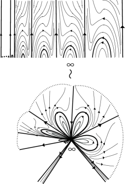
Figure 25. A degenerate singular point with infinitely many parabolic sectors

9. On the Markus-Neumann theorem

As mentioned above, Buendía and López have constructed counterexamples to the Markus-Neumann theorem. Note that one of counterexamples (cf. the figure to the right in Figure 2 [5]) is a toral flow with one singular point and non-recurrent orbits such that a small neighborhood of the singular point consists of two hyperbolic sectors and two parabolic sectors (see Figure 26).

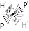
Figure 26. A singular point whose neighborhood consists of two parabolic sectors and two hyperbolic sectors

Moreover, an example of a pair of flows consisting of non-recurrent orbits in a plane in Figure 3 in a paper [26] by Neumann is also a counterexample because flows in the example have no separatrices in the sense of Markus. Indeed, any small neighborhood of $b_{1}$ (resp. $b_{2}$, $c_{1}$, $c_{2}$, $d_{1}$, $d_{2}$) is not a parallel neighborhood satisfying two conditions in definition of separatrix but there is a large neighborhood of it. In addition, Markus-Neumann theorem does not holds for the non-orientable original setting. In fact, the orbit complex of a flow consisting of one axisymmetric rotating spherical flow and two periodic flows on Möbius bands and one of a flow consisting of two axisymmetric rotating flows on projective planes and one periodic flow on a closed annulus are isomorphic, because the orbit space of a connected component is a closed interval and so the orbit spaces of two flows are homeomorphic and because the lift of the orientation double covering of each of them is a flow consisting of two axisymmetric rotating spherical flows and two periodic flows on closed annuli.

As mentioned, additional information is necessary. In fact, there are two spherical flows consisting which are not topologically equivalent but isomorphic as orbit complexes (see Figure 27).

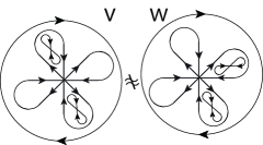
Figure 27. Two spherical flows $v$ and $w$ consisting of closed orbits and homoclinic separatrices which are not topologically equivalent but isomorphic as orbit complexes.

However, we show that orbit complex is a complete invariant for flows of finite type on compact surfaces under the assumption that the multi-saddle connection diagram is the saddle connection diagram containing no non-self-connected separatrices (i.e. each multi-saddle is either a saddle without heteroclinic multi-saddle separatrices or a $\partial$-saddle without separatrices connecting another multi-saddles outside of the same boundary). On the other hand, adding some additional orders, orbit complex becomes complete invariant for flows of finite type on compact surfaces.

9.1. On the Markus-Neumann theorem for flows of finite type

Let $v$ be a flow on a compact surface $S$. We call that an invariant subset $U\subseteq S$ is parallel if $v|_{U}$ is topologically equivalent to either a canonical domain (i.e. an invariant flow box $\mathbb{D}$, an invariant periodic annulus $\mathbb{A}_{+}$, an invariant transverse annulus $\mathbb{A}_{\widetilde{+}}$) as Figure 18, or a periodic torus $\mathbb{T}$. Following [5], we call that a point $x$ is ordinary if it has a parallel neighborhood $U$ such that $\alpha^{\prime}(x)=\alpha^{\prime}(y)$ and $\omega^{\prime}(x)=\omega^{\prime}(y)$ for any point $y\in U$ and that there are exactly two orbits $O_{-}\neq O_{+}$ with $\alpha^{\prime}(x)=\alpha^{\prime}(O_{-})=\alpha^{\prime}(O_{+})$ and $\omega^{\prime}(x)=\omega^{\prime}(O_{-})=\omega^{\prime}(O_{+})$ such that $\partial U=\alpha^{\prime}(x)\cup\omega^{\prime}(x)\cup O_{-}\cup O_{+}$. A point is non-ordinary if it is not ordinary. An orbit is ordinary (resp. non-ordinary) if so are its points. Note that non-ordinary orbit is called a separatrix in the sense of Markus in papers [22, 26, 27, 5]. Denote by $\Sigma_{\mathrm{Sep}}$ the set of non-ordinary points. We show that the set of non-ordinary points correspond to the border point set $\mathop{\mathrm{BD}}(v)$ for a flow of finite type.

Lemma 9.1.

Let $v$ be a flow of finite type on a compact surface $S$. Then $\mathop{\mathrm{BD}}(v)=\Sigma_{\mathrm{Sep}}$.

Proof.

Corollary 5.4 implies that each orbit in $(S-\mathop{\mathrm{BD}}(v))$ has a parallel invariant neighborhood satisfying the conditions in the definition of “ordinary” and so $\mathop{\mathrm{BD}}(v)\supseteq\Sigma_{\mathrm{Sep}}$. On the other hand, we show that $\mathop{\mathrm{BD}}(v)\subseteq\Sigma_{\mathrm{Sep}}$. Indeed, recall that $\mathop{\mathrm{BD}}(v)=\mathop{\mathrm{Bd}}(v)\sqcup\mathop{\mathrm{Per}}_{1}(v)$. Lemma 4.12 implies that $\mathop{\mathrm{BD}}(v)=\mathop{\mathrm{Bd}}(v)\sqcup\mathop{\mathrm{Per}}_{1}(v)=\mathop{\mathrm{Sing}}(v)\sqcup\partial^{-}\mathop{\mathrm{Per}}(v)\sqcup\partial_{\mathop{\mathrm{Per}}(v)}\sqcup\mathop{\mathrm{Per}}_{1}(v)\sqcup\partial^{-}\mathrm{P}(v)\sqcup\mathop{\mathrm{P}_{\mathrm{sep}}}(v)$ consists of finitely many orbits. Since each singular point has no parallel neighborhoods, the singular point set $\mathop{\mathrm{Sing}}(v)$ consists of non-ordinary points. Since each orbit in $\partial^{-}\mathop{\mathrm{Per}}(v)$ is a limit cycle $\gamma$, any its neighborhood $U$ intersects an non-recurrent orbit $O$ with either $\alpha(O)=\alpha^{\prime}(O)=\gamma\neq\emptyset=\alpha^{\prime}(\gamma)$ or $\omega(O)=\omega^{\prime}(O)=\gamma\neq\emptyset=\omega^{\prime}(\gamma)$, and so the union $\partial^{-}\mathop{\mathrm{Per}}(v)$ consists of non-ordinary points. Recall that $\mathop{\mathrm{P}_{\mathrm{sep}}}(v)=\mathop{\mathrm{P}(v)_{\mathrm{ms}}}\sqcup\mathop{\mathrm{P}(v)_{\mathrm{ss}}}\sqcup\mathop{\partial_{\mathrm{P}(v)}}$. Fix a non-recurrent orbit $O$ whose $\omega$-limit set is a multi-saddle $x$. Since each multi-saddle has at most finitely many separatrices, we have $\omega^{\prime}(O)=\{x\}\neq\omega^{\prime}(O^{\prime})$ for all but finitely many orbit $O^{\prime}$ in a neighborhood of $O$. By symmetry, we have $\mathop{\mathrm{P}(v)_{\mathrm{ms}}}\sqcup\mathop{\mathrm{P}(v)_{\mathrm{ss}}}\sqcup\partial^{-}\mathrm{P}(v)\subset\Sigma_{\mathrm{Sep}}$. Since any orbit in $\mathop{\partial_{\mathrm{P}(v)}}\sqcup\partial_{\mathop{\mathrm{Per}}(v)}\sqcup\mathop{\mathrm{Per}}_{1}(v)$ has no parallel neighborhoods, we obtain $\mathop{\partial_{\mathrm{P}(v)}}\sqcup\partial_{\mathop{\mathrm{Per}}(v)}\sqcup\mathop{\mathrm{Per}}_{1}(v)\subseteq\Sigma_{\mathrm{Sep}}$ and so $\mathop{\mathrm{BD}}(v)\subseteq\Sigma_{\mathrm{Sep}}$. ∎

9.1.1. Orders induced by flows

Define a pre-order $\leq_{\alpha}$ (resp. $\leq_{\omega}$) on $S$ as follows:

$$x\leq_{\alpha}y\text{ if }\text{either }x\in\alpha(y)\text{ or }\hat{x}=\hat{y}$$

$$x\leq_{\omega}y\text{ if }\text{either }x\in\omega(y)\text{ or }\hat{x}=\hat{y}$$

Moreover, define a pre-order $\leq_{\alpha}$ (resp. $\leq_{\omega}$) on the power set $2^{S}$ as follows:

$$A\leq_{\alpha}B\text{ if }\text{either }A=B\text{ or }a\leq_{\alpha}b\text{ for any }a\in A,b\in B$$

$$A\leq_{\omega}B\text{ if }\text{either }A=B\text{ or }a\leq_{\omega}b\text{ for any }a\in A,b\in B$$

Define a pre-order $\leq_{\pitchfork}$ for invariant subsets as follows:

$$A\leq_{\pitchfork}B\text{ if }\text{either }A\subseteq\partial_{\pitchfork}B\text{ or }A=B$$

9.1.2. Orbit complex

Recall that the orbit complex is an orbit space with cell structure, fiber type, order structure, and orientability of spirals (see §5 in [27] for details). Let $\pi_{v}:S\to S/v$ be the natural projection. A $1$-cell is the image $\pi_{v}(U)$ of a canonical domain $U$ and a $0$-cell is the image $\pi_{v}(O)$ of an orbit $O$ in $\mathop{\mathrm{BD}}(v)$. In other words, a $1$-cell is a connected component of $\pi_{v}(S-\mathop{\mathrm{BD}}(v))=(S-\mathop{\mathrm{BD}}(v))/v$ and the set of $0$-cells is $\pi_{v}(\mathop{\mathrm{BD}}(v))=\mathop{\mathrm{BD}}(v)/v$. A $1$-cell which is an open interval (resp. a circle) is called an open (resp. closed) 1-cell. Notice that the an open interval (resp. a circle) structure of a $1$-cell is embedded in the orbit space $S/v$. The fiber type of a $i$-cell is either an open interval, a circle, or a point according to the topological type of the fiber of $\pi_{v}$ over a point in the orbit space. In particular, the fiber type of a $1$-cell is either an open interval or a circle. For a canonical domain $U$, the first order structure is a total order on $\partial_{\pitchfork}^{R}U\setminus\mathop{\mathrm{Sing}}(v)$ (resp. $\partial_{\pitchfork}^{L}U\setminus\mathop{\mathrm{Sing}}(v)$), the second order structure is $\leq_{\alpha}|_{\partial U}$ (resp. $\leq_{\omega}|_{\partial U}$), where the restriction $\leq|_{A}:=\leq|_{A\times A}$ of a subset $A$ on a poset $X$ is the restriction as a binary relation. Here the pre-orders are identified as a subsets of $S\times S$ because a binary relation on a set $X$ is a subset of $X\times X$. The third order structure is $\leq_{\alpha}|_{(\partial_{\perp}U)\times U}$ (resp. $\leq_{\omega}|_{U\times\partial_{\perp}U}$). We show that the orbit complex is a complete invariant comparing our invariant by adding two circuit orders $\leq_{\partial_{\perp}^{\alpha}}$ and $\leq_{\partial_{\perp}^{\omega}}$.

Theorem 9.2.

The orbit complex with two circuit orders $\leq_{\partial_{\perp}^{\alpha}}$ and $\leq_{\partial_{\perp}^{\omega}}$ for a flow of finite type on an orientable compact surface is a complete invariant.

Proof.

Fix a flow $v$ of finite type on an orientable compact surface. Recall that our topological invariant for $v$ consists of three abstract multi-graphs $(G^{\mathop{\mathrm{BD}}(v)},G_{\mathop{\mathrm{BD}}(v)}=\mathop{\mathrm{BD}}(v)/v_{\mathrm{ex}},G_{D(v)}=D(v)/v)$ with the labels $L^{\mathrm{BD}(v)}$, $l_{\mathop{\mathrm{BD}}(v)}$, and $l_{D(v)}$, where $L^{\mathrm{BD}(v)}=(\mathcal{O},l^{\mathop{\mathrm{BD}}(v)},\partial^{\mathrm{BD}(v)},\leq^{\mathrm{BD}(v)},\mathcal{D}_{\partial_{\perp}})$. The local orientation $\mathcal{O}$ can be induced by the orientation of the surface. The orbit space implies the abstract multi-saddle connection $D(v)/v$ with the labels $l_{D(v)}$. The $0$-cell structure with fiber type implies the abstract border point set $\mathop{\mathrm{BD}}(v)/v$ and so $G_{\mathrm{BD}(v)}=\mathop{\mathrm{BD}}(v)/v_{\mathrm{ex}}$. The $1$-cell structure with fiber type implies the label $l^{\mathop{\mathrm{BD}}(v)}$. The orbit space with the cell structure implies the dual graph $G^{\mathop{\mathrm{BD}}(v)}$. The fiber structure implies the label $l_{\mathop{\mathrm{BD}}(v)}$. The order structure implies orders $\leq_{\hat{\alpha}}|_{\mathop{\mathrm{BD}}(v)}$ and $\leq_{\hat{\omega}}|_{\mathop{\mathrm{BD}}(v)}$. These orders imply $\leq_{\partial_{\pitchfork}^{R}}$ and $\leq_{\partial_{\pitchfork}^{L}}$. The given circuit orders $\leq_{\partial_{\perp}^{\alpha}}$ and $\leq_{\partial_{\perp}^{\omega}}$ imply the order $\leq^{\mathrm{BD}(v)}=(\leq_{\partial_{\pitchfork}^{R}},\leq_{\partial_{\pitchfork}^{L}},\leq_{\partial_{\perp}^{\alpha}},\leq_{\partial_{\perp}^{\omega}})$. Combining the specialization pre-order for the quotient topology on the orbit space, the orbit structure implies labels $\partial^{\mathrm{BD}(v)}$. The orientability of spirals corresponds to the label $\mathcal{D}_{\partial_{\perp}}$. This means that the orbit complex implies our complete invariant $(G^{\mathop{\mathrm{BD}}(v)},G_{\mathop{\mathrm{BD}}(v)},G_{D(v)},L^{\mathrm{BD}(v)},l_{\mathop{\mathrm{BD}}(v)},l_{D(v)})$. ∎

On the other hand, under the assumption that the multi-saddle connection diagram is the self-connected saddle connection diagram (i.e. saddle connection diagram each of whose multi-saddle is either a saddle without heteroclinic multi-saddle separatrices or a $\partial$-saddle without separatrices connecting another multi-saddles outside of the same boundary), each non-trivial non-periodic circuit in the multi-saddle connection diagram either consists of a saddle with one or two homoclinic separatrices or is a circuit in which $\partial$-saddles and separatrices are arranged alternately. Then the former has a trivial circuit order and the latter circuit order can be reconstructed by orders $\leq_{\hat{\alpha}}|_{\mathop{\mathrm{BD}}(v)}$ and $\leq_{\hat{\omega}}|_{\mathop{\mathrm{BD}}(v)}$. Therefore we obtain the following statement.

Corollary 9.3.

Under the assumption that the multi-saddle connection diagram is the self-connected saddle connection diagram, the orbit complex for a flow of finite type on an orientable compact surface is a complete invariant.

9.2. Proof of Theorem C

Theorem C is followed from Theorem 9.2 and Corollary 9.3.

10. A remark

When flows of finite type on punctured spheres satisfy the self-connectedness of separatrices and the non-degeneracy of singular points, a finite representation of such flows is constructed in [39], which is a generalization of representations used in [36, 37, 38, 46, 49]. In other words, a partial representation for the mapping described in Theorem 8.3 is constructed explicitly.

References

- [1] A. A. Andronov, E. A. Leontovich, I.I. Gordon, A. G. Maǐer, Qualitative theory of dynamic systems of the second order, John Wileg & Sons, 1973.
- [2] Andronov, A. A., and L. S. Pontryagin. Coarse systems, In Dokl. Akad. Nauk SSSR, vol. 14, no. 5, pp. 247–250. 1937.
- [3] Aranson, S., Zhuzhoma, E., Maier’s theorems and geodesic laminations of surface flows J. Dyn. Control. Syst. 2(4), 557–582 (1996).
- [4] S. Kh. Aranson, G. R. Belitsky, E. V. Zhuzhoma, Introduction to the qualitative theory of dynamical systems on surfaces, Trans. Math. Monographs 153, Amer. Math. Soc., 1996.
- [5] Buendía, J. G. E. and López, V. J., On the Markus-Neumann theorem, Journal of Differential Equations, 265(11) (2018), 6036–6047.
- [6] T. M. Cherry, Topological properties of solutions of ordinary differential equations, Amer. J. Math. 59, 957–982, 1937.
- [7] M.Cobo, C. Gutierrez, J. Llibre, Flows without wandering points on compact connected surfaces, Trans. Amer. Math. Soc. 362 (2010), no. 9, 4569–4580.
- [8] J. Franks, Nonsingular Smale Flows on , Topology, 24 (3) (1985) 265–282.
- [9] C. Gardiner, The structure of flows exhibiting non-trivial recurrence on two-dimensional manifolds, J. Diff. Equat. 57(1985), no 1, 138–158.
- [10] C. Gutierrez, Structural stability for flows on the torus with a cross-cap, Trans. Amer. Math. Soc. 241 (1978), 311–320.
- [11] C. Gutierrez, Smoothing continuous flows on S-manifolds and recurrences, Ergod. Th. and Dyn. Sys. 6(1986), 17–44.
- [12] W. Hurewicz, K. Menger, Dimension and Zusammenhangsstuffe, Math. Ann., 100 (1928) 618–633.
- [13] W. Hurewicz, H. Wallman, Dimension Theory, (PMS-4) (Vol. 4), Princeton University Press.
- [14] Kruglov, V., Malyshev, D. and Pochinka, O., Topological classification of -stable flows on surfaces by means of effectively distinguishable multigraphs, Discrete & Continuous Dynamical Systems - A, 38 (9), 4305–4327.
- [15] R. Labarca, M. J. Pacifico. Stability of Morse-Smale vector fields on manifolds with boundary, Topology 29, no. 1 (1990), 57–81.
- [16] G. Levitt, Feuilletages des surfaces, Ann. Inst. Fourier, 32-2 (1982), 179–217.
- [17] López V. J. and López G. S., Empty interior recurrence for continuous flows on surfaces, International Journal of Bifurcation and Chaos, 20(09) (2010), 2897–2913.
- [18] T. Ma, S. Wang, Geometric theory of incompressible flows with applications to fluid dynamics, Mathematical Surveys and Monographs, 119. American Mathematical Society, Providence, RI, 2005.
- [19] N. Markley, The Poincaré-Bendixson Theorem for the Klein Bottle, Trans. Amer. Math. Soc. 135 (1969) 135, 159–165.
- [20] N. Markley, On the number of recurrent orbit closures, Proc. AMS, 25(1970), no 2, 413–416.
- [21] N. Markley, M. Vanderschoot, Recurrent orbits for flows on surfaces, J. Differential Equations, 244(5) (2008), 1210–1229.
- [22] L. Markus, Global structure of ordinary differential equations in the plane, Trans. Amer. Math. Soc. 76 (1954), 127–148.
- [23] A. G. Maǐer, Trajectories on closed orientable surfaces, Mat. Sb. 12 (54) (1943), 71–84
- [24] H. Marzougui, Structure of foliations on 2-manifolds, Illinois J. Math. 42 (1998), No. 3, 398–405.
- [25] H. Marzougui, Some Remarks Concerning the Topological Characterization of Limit Sets for Surface Flows, Canadian Mathematical Bulletin, 54(2) (2011), 311–315.
- [26] Neumann, D. A., Classification of continuous flows on 2-manifolds, Proceedings of the American Mathematical Society (1975), 73–81.
- [27] Neumann, D., and O’Brien, T., Global structure of continuous flows on 2-manifolds, Journal of differential equations, 22(1) (1976), 89–110.
- [28] I. Nikolaev, Non-Wandering Flows on the 2-Manifolds, J. Differential Equations 173 (2001), no. 1, 1–16.
- [29] I. Nikolaev and E. Zhuzhoma, Flows on 2-Dimensional Manifolds, “Lecture Notes in Mathematics,” Vol. 1705, Springer-Verlag, Berlin, 1999.
- [30] A. Oshemkov, V. Sharko, Classification of Morse-Smale flows on two-dimensional manifolds, Mat. sb. 1998. V. 189. No. 8. 93–140.
- [31] M. Peixoto, Structural stability on two-dimensional manifolds, Topology, 1 (1962), 101–120.
- [32] C. Pugh, An improved closing lemma and a general density theorem, Amer. J. Math. 89 (1967), 1010–1021.
- [33] C. Pugh, C. Robinson, The -closing lemma, including Hamiltonians, Ergodic Th. and Dynamical Systems 3 (1983), No. 2, 261–313.
- [34] G. Reeb, Sur certaines propriétés topologiques des variétés feuilletées, Hermann et Cie, 1952.
- [35] K. A. de Rezende, R. D. Franzosa, Lyapunov graphs and flows on surfaces, Trans. Amer. Math. Soc. 340 (1993), 767–784.
- [36] T. Sakajo, Y. Sawamura and T. Yokoyama, Unique encoding for streamline topologies of incompressible and inviscid flows in multiply connected domains, Fluid Dyn. Res., 46 (2014), 031411.
- [37] T. Sakajo and T. Yokoyama, Transitions between streamline topologies of structurally stable Hamiltonian flows in multiply connected domains, Phys. D, 307 (2015), 22–41.
- [38] T. Sakajo and T. Yokoyama, Tree representation of topological streamline patterns of structurally stable 2D Hamiltonian vector fields in multiply connected domains, IMA J. Appl. Math., 83 (2018), 380–411.
- [39] T.Sakajo, T. Yokoyama, Discrete representations of orbit structures of flows for topological data analysis, preprint, arXiv:2010.13434.
- [40] A. J. Schwartz, A generalization of a Poincaré-Bendixson theorem to closed two-dimensional manifolds, Amer. J. Math. 85 (1963), 453–458,
- [41] L.A. Tumarkin, Sur la structure dimensionelle des ensembles fermés C.R. Acad. Paris, 186 (1928) 420–422.
- [42] Urysohn P, . Mémoire sur les multiplicités Cantoriennes, Fundamenta Mathematicae. 1925;1(7):30–137.
- [43] T. Ura, I. Kimura, Sur le courant exterieur a une region invariante; Théorème de Bendixson, Comment. Math. Univers. Sancti Pauli, vol. 8 (1960), 23–39.
- [44] M.H. Vanderschoot, Local connectivity of limit sets, Rocky Mountain J. Math. 33(4) (2003), 1525–1538.
- [45] K. Yano, Asymptotic cycles on two-dimensional manifolds, Adv. St in Pure Math. 1985, 5, 359–377 (Foliations, Proc. Symp, Tokyo, 1983).
- [46] T.Yokoyama, T. Yokoyama, Complete transition diagrams of generic Hamiltonian flows with a few heteroclinic orbits, Discrete Mathematics, Algorithms and Applications, 2021, 13(02), 2150023.
- [47] T. Yokoyama, Topological characterisations for non-wandering surface flows, Proc. Amer. Math. Soc. 144, (2016), 315–323.
- [48] T. Yokoyama, Properness of foliations, Topology Appl. 254 (2019) 171–175.
- [49] T. Yokoyama and T. Sakajo, Word representation of streamline topologies for structurally stable vortex flows in multiply connected domains, Proc. Roy. Soc. A,, 469 (2013), 20120558.