Dynamic Erdős-Rényi graphs

Abstract

We propose two classes of dynamic versions of the classical Erdős-Rényi graph: one in which the transition rates are governed by an external regime process, and one in which the transition rates are periodically resampled. For both models we consider the evolution of the number of edges present, with explicit results for the corresponding moments, functional central limit theorems and large deviations asymptotics.

Keywords:

Random graphs $\circ$ dynamics $\circ$ scaling limits

1 Introduction

Over the past decades, networks have been the subject of an intensive research effort. As networks offer the right framework to model e.g. social, physical, chemical, biological and technological phenomena, various specific aspects have been studied in depth. Arguably among the most studied objects is the Erdős-Rényi graph [6, 7]. In such a random graph $G(n,p)$ there are $n$ vertices, and each of the $N=\binom{n}{2}$ edges is ‘up’ with a fixed probability $p\in(0,1)$ or ‘down’ otherwise. By now there is a sizeable literature on this type of graph, providing detailed insight into its probabilistic properties, an example of a key result being that if the ‘up-probability’ $p$ is larger than $\log n/n$, then the resulting graph is almost surely connected.

The existing literature predominantly focuses on static graphs: the random graph is drawn just once, and does not change over time. In many real-life situations, however, the network structure temporally evolves, with edges appearing and disappearing. In a few recent contributions, first results on such dynamic random graphs have been reported, but the analysis of this class of models is still in its infancy; see e.g. [8, 9, 15], and [1] for an illustration of its use in engineering.

In [15] various dynamic random graph models are discussed, among them a dynamic Erdős-Rényi graph in which all $N$ edges evolve independently. In this model, each edge makes transitions from present to absent and vice versa in a Markovian manner: it exists for an exponential time with parameter $\mu$ (which we refer to as the ‘up-rate’), and disappears for an exponential time with parameter $\lambda$ (the ‘down-rate’). For this model various metrics can be analyzed in closed form. In particular the distribution of the number of edges at time $t$, throughout this paper denoted by $Y(t)$, can be explicitly computed. A special case is that in which no edges exist at $t=0$: then the distribution of $Y(t)$ coincides with the number of edges in a static Erdős-Rényi graph $G(n,p(t))$ (with an up-probability that depends on $t$).

In many applications the model that we just sketched is of limited relevance, as various features that play a role in real-life networks are not covered. To remedy this, in [15] alternative random graph processes were proposed, such as the dynamic counterparts of the configuration model and the stochastic block model. It is noted that a specific property that is often not fulfilled in real networks is that of the edges evolving independently; in practice likely there will be ‘external’ factors that affect all these $N$ processes simultaneously, rendering them dependent. An example is a dynamic random graph in which the values of the up-rate and down-rate are determined by an independent stochastic process (think of temperature in a chemical network, weather conditions in a road traffic network, economic conditions in a financial network, etc.).

Motivated by the above considerations, the focus of this paper is on models in which the edges evolve dependently; the main contribution is that we propose and analyze two such models. In the first model, studied in Section 2, the up-rate and the down-rate of each of the edges are determined by an external, autonomously evolving Markov process $X(t)$, in the sense that at time $t$ these rates (for all edges) are $\lambda_{i}$ and $\mu_{i}$ if $X(t)=i$; this mechanism is usually referred to as regime switching. In the second model, which is analyzed in Section 3, the up-rate and the down-rate (say, $\Lambda$ and $M$) are resampled every $\Delta>0$ time units (and these sampled values then apply to all edges).

In more detail, our findings are the following. The focus is on the probabilistic properties of the process $Y(t)$ that records the number of edges present as a function of time. For both models mentioned above we manage to uniquely characterize its transient and stationary behavior, albeit in a somewhat implicit way: for the first model in terms of a pde for the corresponding probability generating function (pgf), for the second model in terms of a recursion for the pgf. Then we use these characterizations to point out how transient and stationary means can be computed. The next step is to consider scaling limits; under a particular scaling, the process $Y(t)$ satisfies a functional central limit theorem. More specifically, after centering and scaling it converges to an Ornstein-Uhlenbeck (ou) process; interestingly, in [13] it is shown that for certain dynamic Erdős-Rényi graphs that a particular clique-complex related quantity (the ‘Betti number’) is described by an ou process as well. Finally we discuss for both models the corresponding sample-path large deviations, characterizing the models’ rare-event behavior. In Section 4, the results are illustrated by numerical examples.

2 Erdős-Rényi graphs under regime switching

In this section we consider the following model. Let $(X(t))_{t\geqslant 0}$ be an irreducible continuous-time Markov process, typically referred to as the regime process or background process, living on the state space $\{1,\ldots,d\}$. The transition rate matrix corresponding to $(X(t))_{t\geqslant 0}$ is denoted by $Q=(q_{ij})_{i,j=1}^{d}$ and the corresponding invariant distribution by the (column) vector ${\bm{\pi}}$. As before, we consider the situation of $N$ possible vertices. Let $\mu_{i}\geqslant 0$ be the hazard rate of an existing edge becoming inactive when the regime process is in state $i$; likewise, $\lambda_{i}\geqslant 0$ is the hazard rate corresponding with a non-existing edge becoming active. Due to the common regime process the edges are reacting to, the number of links present (denoted by $(Y(t))_{t\geqslant 0}$) evolves according to an interesting dynamic structure.

2.1 Generating function

We start our exposition by studying the (transient and stationary) pgf s

$$\phi_{i}(t,z):={\mathbb{E}}\left(z^{Y(t)}\,1_{\{X(t)=i\}}\right),\>\>\phi_{i}(z):={\mathbb{E}}\left(z^{Y}\,1_{\{X=i\}}\right).$$

We do so by first analyzing $p_{i}(m,t):={\mathbb{P}}(Y(t)=m,X(t)=i),$ by following classical procedures; later we also point out how $p_{i}(m):={\mathbb{P}}(Y=m,X=i)$ can be found. Setting up the Kolmogorov equations, with $q_{i}:=-q_{ii}>0$,

$$p_{i}(m,t+\Delta t) = \sum_{j\not=i}p_{j}(m,t)q_{ji}\,\Delta t$$

$$+\,p_{i}(m+1,t)\mu_{i}(m+1)\Delta t+p_{i}(m-1,t)\lambda_{i}(N-m+1)\Delta t$$

$$+\,p_{i}(m,t)\big{(}1-q_{i}\Delta t-\mu_{i}\,m\,\Delta t-\lambda_{i}\,(N-m)\,\Delta t\big{)}+o(\Delta t),$$

leading to the linear system of differential equations

$$p_{i}^{\prime}(m,t) = \sum_{j=1}^{d}p_{j}(m,t)q_{ji}+p_{i}(m+1,t)\mu_{i}\,(m+1)$$

$$+\,p_{i}(m-1,t)\lambda_{i}\,(N-m+1)-p_{i}(m,t)\mu_{i}\,m-p_{i}(m,t)\lambda_{i}\,(N-m),$$

where $p_{i}(-1,t)$ and $p_{i}(N+1,t)$ are set to $0$. Multiplying by $z^{m}$ and summing over $m=0$ up to $N$, we arrive at the pde

$$\frac{\partial}{{\partial t}}\phi_{i}(t,z) = \sum_{j=1}^{d}\phi_{j}(t,z)q_{ji}+\mu_{i}(1-z)\frac{\partial}{{\partial z}}\phi_{i}(t,z)+$$

$$\lambda_{i}N(z-1)\phi_{i}(t,z)+\lambda_{i}z(1-z)\frac{\partial}{{\partial z}}\phi_{i}(t,z).$$

In stationarity, the left-hand side of the previous display can be equated to 0, thus leading to an ode. We obtain

$$0=\sum_{j=1}^{d}\phi_{j}(z)q_{ji}+\mu_{i}(1-z)\phi_{i}^{\prime}(z)+\lambda_{i}N(z-1)\phi_{i}(z)+\lambda_{i}z(1-z)\phi_{i}^{\prime}(z).$$

2.2 Moments

Following a standard procedure, we can find explicit expressions for all (factorial) moments. To this end, we define $e_{i,k}:={\mathbb{E}}((Y)_{k}1_{\{X=i\}})$, with $(x)_{k}$ denoting $x(x-1)\cdots(x-k+1)$. We obtain the factorial moments by differentiating with respect to $z$ and plugging in $z=1$: in self-evident matrix/vector notation, with $\Lambda:={\rm diag}\{{\bm{\lambda}}\}$ and $M:={\rm diag}\{{\bm{\mu}}\}$,

$${\bm{0}}^{\rm T}={\bm{e}}_{1}^{\rm T}Q-{\bm{e}}_{1}^{\rm T}M+{\bm{\pi}}^{\rm T}\Lambda N-{\bm{e}}_{1}^{\rm T}\Lambda.$$

This leads to ${\mathbb{E}}Y={\bm{e}}_{1}^{\rm T}{\bm{1}}$, with ${\bm{e}}_{1}^{\rm T}=N\cdot{\bm{\pi}}^{\rm T}\Lambda(\Lambda+M-Q)^{-1};$ observe that the mean is proportional to $N$, as expected. This procedure can be found to find a recursion for all factorial moments: by differentiating $k$ times and inserting $z=1$, we obtain, for $k=2,3,\ldots,N$,

$${\bm{0}}^{\rm T}={\bm{e}}_{k}^{\rm T}Q-k\,{\bm{e}}_{k}^{\rm T}M+kN\,{\bm{e}}_{k-1}^{\rm T}\Lambda-k\,{\bm{e}}_{k}^{\rm T}\Lambda-k(k-1)\,{\bm{e}}_{k-1}^{\rm T}\Lambda,$$

and consequently

$${\bm{e}}_{k}^{\rm T}=k\,(N-k+1)\cdot{\bm{e}}_{k-1}^{\rm T}\,\Lambda(k\Lambda+kM-Q)^{-1}.$$

Observe that this recursion can be explicitly solved, as we know ${\bm{e}}_{1}^{\rm T}$; the following result now straightforwardly follows.

Proposition 2.1.

For $k=1,\ldots,N$,

$${\bm{e}}_{k}^{\rm T}=k!\,(N)_{k}\cdot{\bm{\pi}}^{\rm T}\Lambda(\Lambda+M-Q)^{-1}\Lambda(2\Lambda+2M-Q)^{-1}\cdots\Lambda(k\Lambda+kM-Q)^{-1},$$

whereas ${\bm{e}}_{k}^{\rm T}=0$ for $k=N+1,N+2,\ldots$.

Following standard techniques, we can now evaluate all stationary probabilities as well. First, $p_{i}(N)$ follows from the identity ${e}_{i,N}={\mathbb{E}}((Y)_{N}1_{\{X=i\}})=N!\,p_{i}(N).$ We can recursively find the other probabilities $p_{i}(m)$; applying

$$e_{i,N-1}={\mathbb{E}}((Y)_{N-1}1_{\{X=i\}})=(N-1)!\,p_{i}(N-1)+N!\,p_{i}(N),$$

we can express $p_{i}(N-1)$ in terms of $p_{i}(N)$ (and ${e}_{i,N-1}$ and ${e}_{i,N}$). In general $p_{i}(m)$ can be found from $p_{i}(m+1),\ldots,p_{i}(N)$ using

$$e_{i,m}=\sum_{k=m}^{N}(k)_{m}p_{i}(k).$$

Remark 1.

In addition, the transient factorial moments ${\mathbb{E}}((Y(t))_{k}\,1_{\{X(t)=i\}})$ can be (recursively) found; in every step of the recursion a system of linear differential equations (rather than a linear-algebraic equation) needs to be solved; see [12] for a similar procedure in the context of infinite-server queues under regime switching.

2.3 Diffusion results under scaling

In this subsection we impose the scaling $Q\mapsto N^{\delta}Q$, entailing that the regime process is sped up by a factor $N^{\delta}$, with the objective to prove a functional central limit theorem for the resulting limiting process. To get a feeling for how this scaling affects the system’s behavior, we first compute the mean and variance of the stationary number of edges. To this end, we use the following lemma, which is proven in the appendix. In the sequel $D:=({\bm{1}}{\bm{\pi}}^{T}-Q)^{-1}-{\bm{1}}{\bm{\pi}}^{T}$ denotes the deviation matrix. Also $x^{\star}:={\bm{x}}^{\rm T}{\bm{\pi}}$ for ${\bm{x}}\in{\mathbb{R}}^{d}$ and $\Gamma:={\rm diag}\{{\bm{\gamma}}\}=\Lambda+M$. Let ${\bm{\gamma}}:={\bm{\lambda}}+{\bm{\mu}}$ be componentwise positive.

Lemma 2.1.

Define $F_{N,k}:=(k\,\Gamma-NQ)^{-1}$ for $k\in{\mathbb{N}}$. Then, as $N\to\infty$,

$$F_{N,k}=\frac{1}{k}\frac{1}{\gamma^{\star}}{\bm{1}}\,{\bm{\pi}}^{\rm T}+\frac{1}{N}E+O(N^{-2}),\>\>E:=\left(I-\frac{1}{\gamma^{\star}}{\bm{1}}\,{\bm{\pi}}^{\rm T}\Gamma\right)D\left(I-\frac{1}{\gamma^{\star}}{\bm{\gamma}}\,{\bm{\pi}}^{\rm T}\right).$$

Let us first evaluate the mean of $Y$ under this scaling; in the steps below we use ${\bm{\pi}}^{\rm T}\Lambda\,{\bm{1}}=\lambda^{\star}$ and $D{\bm{1}}={\bm{0}}$. From the above lemma, we find, with $\hbox{\vbox{\hrule height=0.4pt\kern 1.72218pt\hbox{\kern-0.39993pt$\varrho$\kern-0.39993pt}}}:=\lambda^{\star}/\gamma^{\star}$,

$${\mathbb{E}}\,Y = N{\bm{\pi}}^{\rm T}\Lambda(\Lambda+M-N^{\delta}Q)^{-1}{\bm{1}}=N{\bm{\pi}}^{\rm T}\Lambda F_{N^{\delta},1}{\bm{1}}$$

$$= N{\bm{\pi}}^{\rm T}\Lambda\left(\frac{1}{\gamma^{\star}}{\bm{1}}{\bm{\pi}}^{\rm T}{\bm{1}}+{N}^{-\delta}\,E{\bm{1}}+O(N^{-2\delta})\right)=N\,\hbox{\vbox{\hrule height=0.4pt\kern 1.72218pt\hbox{\kern-0.39993pt$\varrho$\kern-0.39993pt}}}+O(N^{1-\delta}).$$

Along the same lines,

$$({\mathbb{E}}Y)^{2}=N^{2}\hbox{\vbox{\hrule height=0.4pt\kern 1.72218pt\hbox{\kern-0.39993pt$\varrho$\kern-0.39993pt}}}\,^{2}-N^{2-\delta}\frac{2}{\gamma^{\star}}{\bm{\pi}}^{\rm T}(\Lambda-\hbox{\vbox{\hrule height=0.4pt\kern 1.72218pt\hbox{\kern-0.39993pt$\varrho$\kern-0.39993pt}}}\,\Gamma)D\,\hbox{\vbox{\hrule height=0.4pt\kern 1.72218pt\hbox{\kern-0.39993pt$\varrho$\kern-0.39993pt}}}\,\Gamma{\bm{1}}+o(N^{{\rm max}\{1,2-\delta\}}).$$

In addition, ignoring sublinear terms,

$${\mathbb{E}}Y(Y-1) = 2N(N-1)\,{\bm{\pi}}^{\rm T}\Lambda(\Lambda+M-N^{\delta}Q)^{-1}\Lambda(2\Lambda+2M-N^{\delta}Q)^{-1}{\bm{1}}$$

$$= 2N(N-1)\,{\bm{\pi}}^{\rm T}\Lambda\,F_{N^{\delta},1}\,\Lambda\,F_{N^{\delta},2}{\bm{1}}$$

$$= 2N(N-1)\,{\bm{\pi}}^{\rm T}\Lambda\,\left(\frac{1}{\gamma^{\star}}{\bm{1}}\,{\bm{\pi}}^{\rm T}+\frac{1}{N^{\delta}}E\right)\Lambda\left(\frac{1}{2\gamma^{\star}}{\bm{1}}\,{\bm{\pi}}^{\rm T}+\frac{1}{N^{\delta}}E\right){\bm{1}}.$$

Using the following equalities

$${\bm{\pi}}^{\rm T}\Lambda\,\left(\frac{1}{\gamma^{\star}}{\bm{1}}\,{\bm{\pi}}^{\rm T}\right)\Lambda\left(\frac{1}{2\gamma^{\star}}{\bm{1}}\,{\bm{\pi}}^{\rm T}\right){\bm{1}} = \frac{\hbox{\vbox{\hrule height=0.4pt\kern 1.72218pt\hbox{\kern-0.39993pt$\varrho$\kern-0.39993pt}}}\,^{2}}{2},$$

$${\bm{\pi}}^{\rm T}\Lambda\,E\Lambda\left(\frac{1}{2\gamma^{\star}}{\bm{1}}\,{\bm{\pi}}^{\rm T}\right){\bm{1}} = \frac{1}{2\gamma^{\star}}{\bm{\pi}}^{\rm T}(\Lambda-\hbox{\vbox{\hrule height=0.4pt\kern 1.72218pt\hbox{\kern-0.39993pt$\varrho$\kern-0.39993pt}}}\,\Gamma)D(\Lambda-\hbox{\vbox{\hrule height=0.4pt\kern 1.72218pt\hbox{\kern-0.39993pt$\varrho$\kern-0.39993pt}}}\,\Gamma){\bm{1}},$$

$${\bm{\pi}}^{\rm T}\Lambda\,\left(\frac{1}{\gamma^{\star}}{\bm{1}}\,{\bm{\pi}}^{\rm T}\right)\Lambda E{\bm{1}} = -\frac{1}{\gamma^{\star}}{\bm{\pi}}^{\rm T}(\Lambda-\hbox{\vbox{\hrule height=0.4pt\kern 1.72218pt\hbox{\kern-0.39993pt$\varrho$\kern-0.39993pt}}}\,\Gamma)D\,\hbox{\vbox{\hrule height=0.4pt\kern 1.72218pt\hbox{\kern-0.39993pt$\varrho$\kern-0.39993pt}}}\,\Gamma{\bm{1}},$$

we arrive at

$${\mathbb{E}}Y(Y-1)=N(N-1)\,\hbox{\vbox{\hrule height=0.4pt\kern 1.72218pt\hbox{\kern-0.39993pt$\varrho$\kern-0.39993pt}}}\,^{2}+N^{2-\delta}\frac{1}{\gamma^{\star}}{\bm{\pi}}^{\rm T}(\Lambda-\hbox{\vbox{\hrule height=0.4pt\kern 1.72218pt\hbox{\kern-0.39993pt$\varrho$\kern-0.39993pt}}}\,\Gamma)D(\Lambda-3\,\hbox{\vbox{\hrule height=0.4pt\kern 1.72218pt\hbox{\kern-0.39993pt$\varrho$\kern-0.39993pt}}}\,\Gamma){\bm{1}}+o(N^{{\rm max}\{1,2-\delta\}}).$$

By virtue of the identity ${\mathbb{V}}{\rm ar}\,Y={\mathbb{E}}Y(Y-1)+{\mathbb{E}}Y-({\mathbb{E}}Y)^{2}$, we thus find

$${\mathbb{V}}{\rm ar}\,Y=N\,\hbox{\vbox{\hrule height=0.4pt\kern 1.72218pt\hbox{\kern-0.39993pt$\varrho$\kern-0.39993pt}}}(1-\hbox{\vbox{\hrule height=0.4pt\kern 1.72218pt\hbox{\kern-0.39993pt$\varrho$\kern-0.39993pt}}})+N^{2-\delta}\,v\,+o(N^{{\rm max}\{1,2-\delta\}}),$$ (2.1)

with

$$v:=\frac{1}{\gamma^{\star}}{\bm{\pi}}^{\rm T}(\Lambda-\hbox{\vbox{\hrule height=0.4pt\kern 1.72218pt\hbox{\kern-0.39993pt$\varrho$\kern-0.39993pt}}}\,\Gamma)D(\Lambda-\hbox{\vbox{\hrule height=0.4pt\kern 1.72218pt\hbox{\kern-0.39993pt$\varrho$\kern-0.39993pt}}}\,\Gamma){\bm{1}}.$$

It can be checked that this formula is symmetric, in the sense that it is invariant under swapping ${\bm{\lambda}}$ and ${\bm{\mu}}$, which is in line with ${\mathbb{V}}{\rm ar}\,Y={\mathbb{V}}{\rm ar}\,(N-Y)$; note that $\Lambda-\hbox{\vbox{\hrule height=0.4pt\kern 1.72218pt\hbox{\kern-0.39993pt$\varrho$\kern-0.39993pt}}}\,\Gamma=(1-\hbox{\vbox{\hrule height=0.4pt\kern 1.72218pt\hbox{\kern-0.39993pt$\varrho$\kern-0.39993pt}}})\Lambda-\hbox{\vbox{\hrule height=0.4pt\kern 1.72218pt\hbox{\kern-0.39993pt$\varrho$\kern-0.39993pt}}}M$.

Upon inspecting the asymptotic shape of ${\mathbb{V}}{\rm ar}\,Y$, we observe a dichotomy. For $\delta>1$ the regime process jumps so fast that all edges essentially behave independently, experiencing an ‘effective up-rate’ of $\lambda^{\star}$, and an ‘effective down-rate’ of $\mu^{\star}$, so that in this regime $Y$ is approximated with a Binomial random variable with parameters $N$ and  $\varrho$ . For $\delta<1$ the regime process is relatively slow, and hence affects the variance (which is, as a result, superlinear in $N$).

We now prove a functional central limit theorem. For the moment we focus on the case $\delta=1$; in Remark 3 we comment on what happens when $\delta>1$ or $\delta<1$. Let $P_{1}(\cdot)$ and $P_{2}(\cdot)$ be two independent unit-rate Poisson processes. With $Z_{i}(s):=1_{\{X(s)=i\}}$, and $Y(0)=0$ (remarking that any other starting point can be dealt with similarly),

$$Y(t)=P_{1}\left(\sum_{i=1}^{d}\int_{0}^{t}\lambda_{i}Z_{i}(s)(N-Y(s)){\rm d}s\right)-P_{2}\left(\sum_{i=1}^{d}\int_{0}^{t}\mu_{i}Z_{i}(s)Y(s){\rm d}s\right).$$ (2.2)

The first step is to verify that $Y(t)/N$ converges to $y(t)$, defined as the solution of the integral equation

$$y(t)=\lambda^{\star}\int_{0}^{t}(1-y(s)){\rm d}s-\mu^{\star}\int_{0}^{t}y(s){\rm d}s,$$

i.e., $y(t)=\varrho(t):=\hbox{\vbox{\hrule height=0.4pt\kern 1.72218pt\hbox{\kern-0.39993pt$\varrho$\kern-0.39993pt}}}\cdot(1-e^{-\gamma^{\star}t}).$ Define

$$\hbox{\vbox{\hrule height=0.4pt\kern 1.72218pt\hbox{\kern-0.39993pt$Y$\kern-0.39993pt}}}(t):=\frac{Y(t)-N\varrho(t)}{\sqrt{N}};$$ (2.3)

our objective is to prove that $\hbox{\vbox{\hrule height=0.4pt\kern 1.72218pt\hbox{\kern-0.39993pt$Y$\kern-0.39993pt}}}(\cdot)$ converges to a Gaussian process (and we identify this process). As we follow [2, Section 5], which in turn uses intermediate results of [10], we restrict ourselves to the most important steps.

We know from (2.2) that, for some martingale $K(t)$,

$${\rm d}Y(t)={\bm{\lambda}}^{T}{\bm{Z}}(t)(N-Y(t)){\rm d}t-{\bm{\mu}}^{\rm T}{\bm{Z}}(t)Y(t){\rm d}t+{\rm d}K(t),$$

and therefore

$${\rm d}\hbox{\vbox{\hrule height=0.4pt\kern 1.72218pt\hbox{\kern-0.39993pt$Y$\kern-0.39993pt}}}(t)=\sqrt{N}\big{(}(1-\varrho(t)){\bm{\lambda}}^{\rm T}-\varrho(t){\bm{\mu}}^{\rm T}\big{)}{\bm{Z}}(t){\rm d}t-{\bm{\gamma}}^{\rm T}{\bm{Z}}(t)\hbox{\vbox{\hrule height=0.4pt\kern 1.72218pt\hbox{\kern-0.39993pt$Y$\kern-0.39993pt}}}(t){\rm d}t+\frac{{\rm d}K(t)}{\sqrt{N}}-\sqrt{N}\varrho^{\prime}(t){\rm d}t.$$

Now define $W(t):=e^{Z_{+}(t)}\hbox{\vbox{\hrule height=0.4pt\kern 1.72218pt\hbox{\kern-0.39993pt$Y$\kern-0.39993pt}}}(t),$ where ${Z}_{+}(t):=\int_{0}^{t}{\bm{\gamma}}^{\rm T}{\bm{Z}}(s){\rm d}s,$ so that,

$${\rm d}W(t)=e^{Z_{+}(t)}\left(\sqrt{N}\big{(}(1-\varrho(t)){\bm{\lambda}}^{\rm T}-\varrho(t){\bm{\mu}}^{\rm T}\big{)}{\bm{Z}}(t){\rm d}t+\frac{{\rm d}K(t)}{\sqrt{N}}-\sqrt{N}\varrho^{\prime}(t){\rm d}t\right).$$

Observing that $\big{(}(1-\varrho(t)){\bm{\lambda}}^{\rm T}-\varrho(t){\bm{\mu}}^{\rm T}\big{)}{\bm{\pi}}=\varrho^{\prime}(t),$ and recalling that ${\bm{\gamma}}={\bm{\lambda}}+{\bm{\mu}}$, the equality in the previous display simplifies to

$${\rm d}W(t)=e^{Z_{+}(t)}\left(\sqrt{N}\big{(}{\bm{\lambda}}^{\rm T}-\varrho(t){\bm{\gamma}}^{\rm T}\big{)}({\bm{Z}}(t)-{\bm{\pi}}){\rm d}t+\frac{{\rm d}K(t)}{\sqrt{N}}\right).$$

We now consider the two terms in the previous display separately. As was established in [2, 10], for the first term, as $N\to\infty$,

$$\int_{0}^{\cdot}\sqrt{N}e^{Z_{+}(s)}\big{(}{\bm{\lambda}}^{\rm T}-\varrho(s){\bm{\gamma}}^{\rm T}\big{)}({\bm{Z}}(s)-{\bm{\pi}}){\rm d}s\to\int_{0}^{\cdot}e^{\gamma^{\star}s}{\rm d}G(s),$$

where $G(\cdot)$ satisfies

$$\langle G\rangle_{t}=g(t):=2\int_{0}^{t}{\bm{\pi}}^{\rm T}(\Lambda-\varrho(s)\Gamma)D(\Lambda-\varrho(s)\Gamma){\bm{1}}{\rm d}s.$$ (2.4)

Also as in [2, 10], the second term obeys, as $N\to\infty$,

$$\int_{0}^{\cdot}\frac{1}{\sqrt{N}}e^{Z_{+}(s)}{\rm d}K(s)\to\int_{0}^{\cdot}e^{\gamma^{\star}s}{\rm d}H(s),$$

where $H(\cdot)$ satisfies (using the relation between $K(\cdot)$ and the Poisson processes $P_{1}(\cdot)$ and $P_{2}(\cdot)$)

$$\langle H\rangle_{t}=h(t):=\int_{0}^{t}\lambda^{\star}(1-\varrho(s)){\rm d}s+\int_{0}^{t}\mu^{\star}\varrho(s){\rm d}s.$$ (2.5)

Combining the two terms studied above, it thus follows that, as $N\to\infty$, $W(\cdot)$ weakly converges to $W_{\infty}(\cdot)$, which is the solution to the stochastic differential equation, with $B(\cdot)$ a standard Brownian motion,

$${\rm d}W_{\infty}(t)=e^{\gamma^{\star}t}\sqrt{g^{\prime}(t)+h^{\prime}(t)}\,{\rm d}B(t).$$ (2.6)

Translating this back in terms of a stochastic differential equation, again mimicking the line of reasoning of [2, 10], we obtain the following result.

Theorem 2.1.

$\hbox{\vbox{\hrule height=0.4pt\kern 1.72218pt\hbox{\kern-0.39993pt$Y$\kern-0.39993pt}}}(\cdot)$ converges weakly to $\hbox{\vbox{\hrule height=0.4pt\kern 1.72218pt\hbox{\kern-0.39993pt$Y$\kern-0.39993pt}}}_{\infty}(\cdot)$, which is the solution to the stochastic differential equation

$${\rm d}\hbox{\vbox{\hrule height=0.4pt\kern 1.72218pt\hbox{\kern-0.39993pt$Y$\kern-0.39993pt}}}_{\infty}(t)=-\gamma^{\star}\,\hbox{\vbox{\hrule height=0.4pt\kern 1.72218pt\hbox{\kern-0.39993pt$Y$\kern-0.39993pt}}}_{\infty}(t)\,{\rm d}t+\sqrt{g^{\prime}(t)+h^{\prime}(t)}\,{\rm d}B(t),$$ (2.7)

with $g(\cdot)$ and $h(\cdot)$ given by $(\ref{defg1})$ and $(\ref{defh1})$, respectively.

Remark 2.

Using the behavior of $g^{\prime}(t)$ and $h^{\prime}(t)$ for $t$ large, we conclude that for large values of $t$ (‘in stationarity’), this stochastic differential equation reads

$${\rm d}\hbox{\vbox{\hrule height=0.4pt\kern 1.72218pt\hbox{\kern-0.39993pt$Y$\kern-0.39993pt}}}_{\infty}(t)=-\gamma^{\star}\,\hbox{\vbox{\hrule height=0.4pt\kern 1.72218pt\hbox{\kern-0.39993pt$Y$\kern-0.39993pt}}}_{\infty}(t)\,{\rm d}t+\sqrt{2\gamma^{\star}\,\hbox{\vbox{\hrule height=0.4pt\kern 1.72218pt\hbox{\kern-0.39993pt$\varrho$\kern-0.39993pt}}}\,(1-\hbox{\vbox{\hrule height=0.4pt\kern 1.72218pt\hbox{\kern-0.39993pt$\varrho$\kern-0.39993pt}}})+2\gamma^{\star}\,v}\,{\rm d}B(t),$$

which defines an ou process with mean $0$ and variance $\hbox{\vbox{\hrule height=0.4pt\kern 1.72218pt\hbox{\kern-0.39993pt$\varrho$\kern-0.39993pt}}}\,(1-\hbox{\vbox{\hrule height=0.4pt\kern 1.72218pt\hbox{\kern-0.39993pt$\varrho$\kern-0.39993pt}}})+v$; note that this aligns with what we found, plugging in $\delta=1$, in (2.1).

Remark 3.

When $\delta<1$, the $\sqrt{N}$ in the definition of (2.2) needs to be replaced by $N^{\delta/2}$; it is readily checked that in the limiting stochastic differential equation (2.7) we then just have $g^{\prime}(t)$ below the square-root sign. On the contrary, if $\delta>1$ then the definition of (2.2) remains unchanged, but below the square-root sign in (2.7) we only have $h^{\prime}(t)$.

2.4 Large deviations results under scaling

Where we above discussed the diffusion behavior of the process under study, we now consider rare events. We again focus on the scaling corresponding to $\delta=1$, following the setup of [11]. Intuitively, the rare-event behavior is decomposed into the effect of the regime process, and that of the edge dynamics conditional on the regime process.

Let ${\bm{g}}(\cdot)$ be in $U_{T}$, defined as the set of non-negative $d$-dimensional functions such that the $g_{i}(s)$ sum to $1$, for all $s\in[0,T]$. Then

$${\mathbb{J}}_{T}({\bm{g}}):=\int_{0}^{T}\sup_{{\bm{u}}\geqslant{\bm{0}}}\left(-\sum_{i=1}^{d}\frac{(Q{\bm{u}})_{i}}{u_{i}}g_{i}(s)\right){\rm d}s.$$

In addition,

$$\Lambda_{x,{\bm{g}}}(\vartheta):=\sum_{i=1}^{d}g_{i}\left(x\lambda_{i}(e^{\vartheta}-1)+(1-x)\mu_{i}(e^{-\vartheta}-1)\right).$$

Based on the findings in [11], one anticipates a sample-path ldp (of ‘Mogulskii type’; cf. [4, Thm. 5.2]), with local rate function

$$I_{x,{\bm{g}}}(y):=\sup_{\vartheta}\left(\vartheta y-\Lambda_{x,{\bm{g}}}(\vartheta)\right).$$

This concretely means that, with $Y^{\circ}(t):=N^{-1}Y(t)$ and $t\in[0,T]$, and under mild regularity conditions on the set $A$,

$$\lim_{N\to\infty}\frac{1}{N}\log{\mathbb{P}}(Y^{\circ}(\cdot)\in A)=-\inf_{f\in A}{\mathbb{I}}_{T}(f),$$

with

$${\mathbb{I}}_{T}(f):=\inf_{{\bm{g}}(\cdot)\in U_{T}}\left(\int_{0}^{T}I_{f(s),{\bm{g}}(s)}(f^{\prime}(s)){\rm d}s+{\mathbb{J}}_{T}({\bm{g}})\right).$$

A formal derivation of this ldp is beyond the scope of this paper.

3 Erdős-Rényi graphs with resampling

An alternative dynamic Erdős-Rényi model (in discrete time) can be defined as follows; we refer to it as a Erdős-Rényi graph with resampling. Let the $N$ edges alternate between two states: the edge has the value $0$ when the corresponding edge is absent and $1$ when it exists. In slot $m$, let the transition matrix of the presence of any of the $N$ edges be given by

$$\left(\begin{array}[]{cc}P_{m}&1-P_{m}\\ 1-R_{m}&R_{m}\end{array}\right),$$

where the sequence $(P_{m},R_{m})_{m\in{\mathbb{N}}}$ consists of i.i.d. vectors in $(0,1)^{2}$; we note that $P_{m}$ and $R_{m}$ (for a given time $m$, that is) are not necessarily assumed independent. It is stressed that the samples in slot $m$, i.e., $P_{m}$ and $R_{m}$, hold for any of the edges — as a consequence, the individual edges (each of them alternating between absent and present) evolve dependently, as intended.

In this section we find the counterparts for the resampling model of all results that we derived for the regime switching model of Section 2. To make notation compact, let $(P,R)$ denote a generic sample of $(P_{m},R_{m})$.

3.1 Generating function

Let us now analyze the object $\varphi_{k}(z):={\mathbb{E}}\left(z^{Y_{m}}\,|\,Y_{m-1}=k\right).$ Realize that $Y_{m}$ is the sum of (i) the edges that were present at time $m-1$ and still are at $m$, and (ii) the edges that were not there at $m-1$ but do appear at $m$. Both obey a binomial distribution (with appropriately chosen parameters). More precisely,

$$\varphi_{k}(z)={\mathbb{E}}\left(\sum_{\ell=0}^{N-k}\binom{N-k}{\ell}(1-P_{m})^{\ell}P_{m}^{N-k-\ell}z^{\ell}\cdot\sum_{\ell=0}^{k}\binom{k}{\ell}R_{m}^{\ell}(1-R_{m})^{k-\ell}z^{\ell}\right),$$

which simplifies to

$${\mathbb{E}}\left(\left((1-P_{m})z+P_{m}\right)^{N-k}\cdot\left(R_{m}z+1-R_{m}\right)^{k}\right).$$

Now consider the stationary random variable $Y$, through its $z$-transform $\varphi(z):={\mathbb{E}}\,z^{Y}.$ Based on the above computation, we have found the following fixed-point equation:

$$\varphi(z)={\mathbb{E}}\left(((1-P)z+P)^{N}\,\varphi\left(\frac{Rz+1-R}{(1-P)z+P}\right)\right).$$ (3.1)

3.2 Moments

In this subsection, we compute the mean, variance and correlation in stationarity.

Mean. Let us first compute ${\mathbb{E}}\,Y$, by differentiating both sides to $z$ and plugging in $z=1$. To this end, we define

$$\psi_{1}(z):=((1-P)z+P)^{N},\>\>\>\psi_{2}(z):=\varphi\left(\frac{Rz+1-R}{(1-P)z+P}\right).$$

We first compute a number of quantities that we need in the sequel. It takes routine calcutations to conclude that

$$\psi_{1}^{\prime}(z) = (1-P)N((1-P)z+P)^{N-1},$$

$$\psi_{1}^{\prime\prime}(z) = (1-P)^{2}N(N-1)((1-P)z+P)^{N-2},$$

$$\psi^{\prime}_{2}(z) = \frac{P+R-1}{((1-P)z+P)^{2}}\varphi^{\prime}\left(\frac{Rz+1-R}{(1-P)z+P}\right),$$

and

$$\psi_{2}^{\prime\prime}(z) = -2\frac{(P+R-1)(1-P)}{((1-P)z+P)^{3}}\varphi^{\prime}\left(\frac{Rz+1-R}{(1-P)z+P}\right)+$$

$$\frac{(P+R-1)^{2}}{((1-P)z+P)^{4}}\varphi^{\prime\prime}\left(\frac{Rz+1-R}{(1-P)z+P}\right).$$

As a consequence,

$$\psi^{\prime}_{1}(1)=(1-P)N,\>\>\>\psi^{\prime\prime}_{1}(1)=(1-P)^{2}N(N-1),\>\>\>\psi^{\prime}_{2}(1)=(P+R-1)\varphi^{\prime}(1),$$

and

$$\psi_{2}^{\prime\prime}(1)=-2(P+R-1)(1-P)\varphi^{\prime}(1)+(P+R-1)^{2}\varphi^{\prime\prime}(1).$$

Regarding the first moment of $Y$, we obtain the equation $\alpha:=\varphi^{\prime}(1)={\mathbb{E}}\,\psi_{1}^{\prime}(1)+{\mathbb{E}}\,\psi_{2}^{\prime}(1),$ or equivalently $\alpha=N(1-{\mathbb{E}}\,P)+\alpha({\mathbb{E}}\,P+{\mathbb{E}}\,R-1),$ and hence

$$\alpha=N\,\frac{1-{\mathbb{E}}\,P}{2-{\mathbb{E}}\,P-{\mathbb{E}}\,R}.$$ (3.2)

Variance. We now evaluate the quantity

$$\beta:={\mathbb{E}}\,Y(Y-1)=\varphi^{\prime\prime}(1)={\mathbb{E}}\,\psi_{1}^{\prime\prime}(1)+2\,{\mathbb{E}}\,\psi_{1}^{\prime}(1)\psi_{2}^{\prime}(1)+{\mathbb{E}}\,\psi_{2}^{\prime\prime}(1).$$

We thus obtain that $\beta$ equals

$$N(N-1)\,{\mathbb{E}}\left((1-P)^{2}\right)+2(N-1)\,\alpha\,{\mathbb{E}}\left((P+R-1)(1-P)\right)+\beta\,{\mathbb{E}}\left((P+R-1)^{2}\right),$$

and therefore

$$\beta=\frac{N(N-1)\,{\mathbb{E}}\left((1-P)^{2}\right)+2(N-1)\,\alpha\,{\mathbb{E}}\left((P+R-1)(1-P)\right)}{1-{\mathbb{E}}\left((P+R-1)^{2}\right)}.$$

As a consequence, ${\mathbb{V}}{\rm ar}\,Y$ equals

$$\alpha-\alpha^{2}+\frac{N(N-1)\,{\mathbb{E}}\left((1-P)^{2}\right)+2(N-1)\,\alpha\,{\mathbb{E}}\left((P+R-1)(1-P)\right)}{1-{\mathbb{E}}\left((P+R-1)^{2}\right)}.$$

It takes an elementary but tedious computation to very that if $P$ and $R$ equal (deterministically) $p$ and $r$, respectively, then this variance reduces to $N\pi_{0}\pi_{1}$, as desired.

We also conclude that ${\mathbb{V}}{\rm ar}\,Y$ grows essentially quadratic in $N$. Indeed, it follows by standard computations that, with $\hbox{\vbox{\hrule height=0.4pt\kern 1.72218pt\hbox{\kern-0.39993pt$P$\kern-0.39993pt}}}:=1-P$ and $\hbox{\vbox{\hrule height=0.4pt\kern 1.72218pt\hbox{\kern-0.39993pt$R$\kern-0.39993pt}}}:=1-R$,

$${\mathbb{V}}{\rm ar}\,Y=\gamma_{1}N^{2}+\gamma_{2}N,$$ (3.3)

where

$$\gamma_{1}=\frac{{\mathbb{E}}(\hbox{\vbox{\hrule height=0.4pt\kern 1.72218pt\hbox{\kern-0.39993pt$R$\kern-0.39993pt}}}^{2})({\mathbb{E}}\,\hbox{\vbox{\hrule height=0.4pt\kern 1.72218pt\hbox{\kern-0.39993pt$P$\kern-0.39993pt}}})^{2}-2\,{\mathbb{E}}(\hbox{\vbox{\hrule height=0.4pt\kern 1.72218pt\hbox{\kern-0.39993pt$P$\kern-0.39993pt}}}\hbox{\vbox{\hrule height=0.4pt\kern 1.72218pt\hbox{\kern-0.39993pt$R$\kern-0.39993pt}}}){\mathbb{E}}\,\hbox{\vbox{\hrule height=0.4pt\kern 1.72218pt\hbox{\kern-0.39993pt$P$\kern-0.39993pt}}}\,{\mathbb{E}}\,\hbox{\vbox{\hrule height=0.4pt\kern 1.72218pt\hbox{\kern-0.39993pt$R$\kern-0.39993pt}}}+{\mathbb{E}}(\hbox{\vbox{\hrule height=0.4pt\kern 1.72218pt\hbox{\kern-0.39993pt$P$\kern-0.39993pt}}}^{2})({\mathbb{E}}\,\hbox{\vbox{\hrule height=0.4pt\kern 1.72218pt\hbox{\kern-0.39993pt$R$\kern-0.39993pt}}})^{2}}{\left(1-{\mathbb{E}}\left((\hbox{\vbox{\hrule height=0.4pt\kern 1.72218pt\hbox{\kern-0.39993pt$P$\kern-0.39993pt}}}+\hbox{\vbox{\hrule height=0.4pt\kern 1.72218pt\hbox{\kern-0.39993pt$R$\kern-0.39993pt}}}-1)^{2}\right)\right)\left({\mathbb{E}}\,\hbox{\vbox{\hrule height=0.4pt\kern 1.72218pt\hbox{\kern-0.39993pt$P$\kern-0.39993pt}}}+{\mathbb{E}}\,\hbox{\vbox{\hrule height=0.4pt\kern 1.72218pt\hbox{\kern-0.39993pt$R$\kern-0.39993pt}}}\right)^{2}},$$

and

$$\gamma_{2}=\frac{-\,{\mathbb{E}}(\hbox{\vbox{\hrule height=0.4pt\kern 1.72218pt\hbox{\kern-0.39993pt$R$\kern-0.39993pt}}}^{2})\,{\mathbb{E}}\,\hbox{\vbox{\hrule height=0.4pt\kern 1.72218pt\hbox{\kern-0.39993pt$P$\kern-0.39993pt}}}+2\,{\mathbb{E}}\,\hbox{\vbox{\hrule height=0.4pt\kern 1.72218pt\hbox{\kern-0.39993pt$P$\kern-0.39993pt}}}\,{\mathbb{E}}\,\hbox{\vbox{\hrule height=0.4pt\kern 1.72218pt\hbox{\kern-0.39993pt$R$\kern-0.39993pt}}}-{\mathbb{E}}(\hbox{\vbox{\hrule height=0.4pt\kern 1.72218pt\hbox{\kern-0.39993pt$P$\kern-0.39993pt}}}^{2})\,{\mathbb{E}}\,\hbox{\vbox{\hrule height=0.4pt\kern 1.72218pt\hbox{\kern-0.39993pt$R$\kern-0.39993pt}}}}{\left(1-{\mathbb{E}}\left((\hbox{\vbox{\hrule height=0.4pt\kern 1.72218pt\hbox{\kern-0.39993pt$P$\kern-0.39993pt}}}+\hbox{\vbox{\hrule height=0.4pt\kern 1.72218pt\hbox{\kern-0.39993pt$R$\kern-0.39993pt}}}-1)^{2}\right)\right)\left({\mathbb{E}}\,\hbox{\vbox{\hrule height=0.4pt\kern 1.72218pt\hbox{\kern-0.39993pt$P$\kern-0.39993pt}}}+{\mathbb{E}}\,\hbox{\vbox{\hrule height=0.4pt\kern 1.72218pt\hbox{\kern-0.39993pt$R$\kern-0.39993pt}}}\right)}.$$

Notice that $\gamma_{1}$ and $\gamma_{2}$ are symmetric in $P$ and $R$, as desired, and observe that $\gamma_{1}\geq 0$ (with equality only if $P$ and $R$ are deterministic). We conclude that no standard CLT applies (which would require that ${\mathbb{V}}{\rm ar}\,Y$ grows linearly in $N$) unless $P$ and $R$ are deterministic.

Correlation. We now focus on computing the limit of covariance ${\mathbb{C}}{\rm ov}(Y_{m},Y_{m+1})$ as $m\to\infty.$ Observe that

$$\lim_{m\to\infty}{\mathbb{C}}{\rm ov}(Y_{m},Y_{m+1})=\lim_{m\to\infty}\sum_{k=0}^{N}k\,{\mathbb{E}}(Y_{m+1}\,|\,Y_{m}=k)\,{\mathbb{P}}(Y_{m}=k)-({\mathbb{E}}\,Y)^{2},$$

which, in self-evident notation, reads

$$\sum_{k=0}^{N}k\,{\mathbb{E}}({\mathbb{B}}{\rm in}(k,R))\,{\mathbb{P}}(Y=k)+\sum_{k=0}^{N}k\,{\mathbb{E}}({\mathbb{B}}{\rm in}(N-k,1-P))\,{\mathbb{P}}(Y=k)-({\mathbb{E}}\,Y)^{2}.$$

This reduces to

$$\,{\mathbb{E}}R\,\sum_{k=0}^{N}k^{2}\,{\mathbb{P}}(Y=k)+(1-\,{\mathbb{E}}P)\sum_{k=0}^{N}k(N-k)\,{\mathbb{P}}(Y=k)-({\mathbb{E}}\,Y)^{2},$$

so that we obtain

$$\lim_{m\to\infty}{\mathbb{C}}{\rm ov}(Y_{m},Y_{m+1})=({\mathbb{E}}P+{\mathbb{E}}R-1){\mathbb{E}}(Y^{2})+(1-\,{\mathbb{E}}P)N\,{\mathbb{E}}\,Y-({\mathbb{E}}\,Y)^{2},$$

which we can evaluate from the expressions for ${\mathbb{E}}\,Y$ and ${\mathbb{V}}{\rm ar}\,Y.$

3.3 Diffusion results under scaling

We now consider the following scaling: for some $\delta>0$ we put

$$P=1-\eta/N^{\delta},\>\>\>\>R=1-\zeta/N^{\delta},$$ (3.4)

where $\eta$ and $\zeta$ are non-negative random variables. The resulting model has some built-in ‘inertia’: for $N$ large, the process has the inclination to stay in the same configuration. The mean number of vertices is $N\,\hbox{\vbox{\hrule height=0.4pt\kern 1.72218pt\hbox{\kern-0.39993pt$\varrho$\kern-0.39993pt}}},$ with

$$\hbox{\vbox{\hrule height=0.4pt\kern 1.72218pt\hbox{\kern-0.39993pt$\varrho$\kern-0.39993pt}}}:=\frac{{\mathbb{E}}\,\eta}{{\mathbb{E}}\,\eta+{\mathbb{E}}\,\zeta},$$

irrespective of the value of $\delta$. When analyzing the variance, however, the revealing issue is that the value of $\delta$ has crucial impact. More specifically, a minor computation tells us that ${\mathbb{V}}{\rm ar}\,Y$ essentially reads

$$N\,\hbox{\vbox{\hrule height=0.4pt\kern 1.72218pt\hbox{\kern-0.39993pt$\varrho$\kern-0.39993pt}}}\,(1-\,\hbox{\vbox{\hrule height=0.4pt\kern 1.72218pt\hbox{\kern-0.39993pt$\varrho$\kern-0.39993pt}}}\,)+N^{2-\delta}\frac{{\mathbb{E}}(\zeta^{2})({\mathbb{E}}\,\eta)^{2}-2\,{\mathbb{E}}(\eta\zeta){\mathbb{E}}\,\eta\,{\mathbb{E}}\,\zeta+{\mathbb{E}}(\eta^{2})({\mathbb{E}}\,\zeta)^{2}}{2({\mathbb{E}}\,\eta+{\mathbb{E}}\,\zeta)^{3}}.$$

Note that, due to the inertia that we incorporated, the variance is smaller than in the unscaled model, where the variance was effectively proportional to $N^{2}$. Observe from the above expression that there is a dichotomy that resembles the one we came across in Section 2, with some sort of transition at $\delta=1.$ For $\delta>1$ the standard deviation scales as $\sqrt{N}$, whereas for $\delta<1$ it scales as $N^{1-\delta/2}$. An intuitive explanation is that in the regime of relatively few transitions (i.e., $\delta>1$) the system’s inertia is so strong that its steady-state essentially behaves as an Erdős-Rényi graph with the probability that an edge exists being given by  $\varrho$ . In the regime with relatively many transitions (i.e., $\delta<1$), on the contrary, the (co-)variances play a role, in the sense that the increased variability caused by the resampling has impact; the limiting object is not of Erdős-Rényi-type.

Along the same lines, an elementary computation yields that the covariance between the numbers of edges at two subsequent epochs (in stationarity) behaves as

$${\mathbb{V}}{\rm ar}\,Y\left(1-\frac{{\mathbb{E}}\,\eta+{\mathbb{E}}\,\zeta}{N^{\delta}}\right);$$

this correlation coefficient essentially reads $1-({{\mathbb{E}}\,\eta+{\mathbb{E}}\,\zeta}){N^{-\delta}}$ (for $N$ large).

A related continuous-time model. In the remainder of this subsection we consider a specific explicit continuous-time model in which we can embed the discrete-time model discussed above, and in particular the scaling (3.4). To this end, we first describe the model without scaling, and then include the scaling.

Let, at time $s$, $M(s)\geqslant 0$ be the hazard rate of an existing vertex becoming inactive; likewise, $\Lambda(s)\geqslant 0$ is the hazard rate corresponding with a non-existing vertex becoming active. Here $M(s)$ and $\Lambda(s)$ are piecewise constant stochastic processes: for some $\Delta>0$,

$$\Lambda(s)=\Lambda_{i}\,1_{\{(i-1)\Delta\leqslant s<i\Delta\}},\>\>\>M(s)=M_{i}\,1_{\{(i-1)\Delta\leqslant s<i\Delta\}},$$

where $(M_{i},\Lambda_{i})_{i\in{\mathbb{N}}}$ is a sequence of i.i.d. bivariate random vectors such that both ${\mathbb{V}}{\rm ar}\,\Lambda$ and ${\mathbb{V}}{\rm ar}\,M$ are finite. Let $Y(t)$ be the number of vertices at time $t$, and $Y$ its stationary counterpart. As it turns out, we can reuse quite a few results from the previous subsections, using the identification $Y(m\Delta)=Y_{m}.$ In particular, it is seen that $\varphi(z):={\mathbb{E}}\,z^{Y}$ satisfies (3.1), with

$$P:=\frac{M}{\Lambda+M}+\frac{\Lambda}{\Lambda+M}e^{-(\Lambda+M)\Delta},\>\>R:=\frac{\Lambda}{\Lambda+M}+\frac{M}{\Lambda+M}e^{-(\Lambda+M)\Delta}.$$

We thus obtain from (3.2)

$${\mathbb{E}}\,Y=N\,{\mathbb{E}}\left(\frac{\Lambda}{\Lambda+M}\left(1-e^{-(\Lambda+M)\Delta}\right)\right)\left/{\mathbb{E}}\left(1-e^{-(\Lambda+M)\Delta}\right)\right.$$

Similarly, we can compute the variance by (3.3).

Now we describe how to scale this model. The idea is to scale $\Delta\mapsto 1/N^{\delta}$, and to consider the regime in which we let $N$ grow large, i.e., the transition rates are frequently resampled (and simultaneously the number of potential edges $N$ grows). It is immediate that $P$ and $R$ fulfill (3.4) with $\eta=\Lambda$ and $\zeta=M.$ We obtain that ${\mathbb{E}}\,Y$ tends to $\hbox{\vbox{\hrule height=0.4pt\kern 1.72218pt\hbox{\kern-0.39993pt$\varrho$\kern-0.39993pt}}}:={\mathbb{E}}\,\Lambda/{\mathbb{E}}\,\Gamma$, where $\Gamma:=\Lambda+M$. In addition, ${\mathbb{V}}{\rm ar}\,Y$ satisfies the expansion $N\,\hbox{\vbox{\hrule height=0.4pt\kern 1.72218pt\hbox{\kern-0.39993pt$\varrho$\kern-0.39993pt}}}\,(1-\,\hbox{\vbox{\hrule height=0.4pt\kern 1.72218pt\hbox{\kern-0.39993pt$\varrho$\kern-0.39993pt}}}\,)+N^{2-\delta}v+o(N^{\max\{1,2-\delta\}})$, where

$$v := \frac{1}{2\,{\mathbb{E}}\,\Gamma}\left(\,\hbox{\vbox{\hrule height=0.4pt\kern 1.72218pt\hbox{\kern-0.39993pt$\varrho$\kern-0.39993pt}}}\,^{2}\,{\mathbb{V}}{\rm ar}\,M-2\,\hbox{\vbox{\hrule height=0.4pt\kern 1.72218pt\hbox{\kern-0.39993pt$\varrho$\kern-0.39993pt}}}\,(1-\,\hbox{\vbox{\hrule height=0.4pt\kern 1.72218pt\hbox{\kern-0.39993pt$\varrho$\kern-0.39993pt}}}\,)\,{\mathbb{C}}{\rm ov}\,(\Lambda,M)+(1-\,\hbox{\vbox{\hrule height=0.4pt\kern 1.72218pt\hbox{\kern-0.39993pt$\varrho$\kern-0.39993pt}}}\,)^{2}\,{\mathbb{V}}{\rm ar}\,\Lambda\right)$$

$$= \frac{1}{2\,{\mathbb{E}}\,\Gamma}{\mathbb{V}}{\rm ar}\left(\Lambda-\,\hbox{\vbox{\hrule height=0.4pt\kern 1.72218pt\hbox{\kern-0.39993pt$\varrho$\kern-0.39993pt}}}\,\Gamma\right).$$

The proof of a functional central limit theorem is very similar to the one for the regime switching model in Section 2; we therefore restrict ourselves to the key steps. With $P_{1}(\cdot)$ and $P_{2}(\cdot)$ as before,

$$Y(t)=P_{1}\left(\int_{0}^{t}\Lambda(s)(N-Y(s)){\rm d}s\right)-P_{2}\left(\int_{0}^{t}M(s)Y(s){\rm d}s\right),$$

so that, for some martingale $K(t)$,

$${\rm d}Y(t)=\Lambda(t)(N-Y(t)){\rm d}t-M(t)Y(t){\rm d}t+{\rm d}K(t).$$

Then $\hbox{\vbox{\hrule height=0.4pt\kern 1.72218pt\hbox{\kern-0.39993pt$Y$\kern-0.39993pt}}}(t)$ is defined as in (2.3), with $\varrho(t):=\hbox{\vbox{\hrule height=0.4pt\kern 1.72218pt\hbox{\kern-0.39993pt$\varrho$\kern-0.39993pt}}}\cdot(1-\exp(-t\,{\mathbb{E}}\,\Gamma)).$ We define, with $\Gamma(s)=\Lambda(s)+M(s)$,

$$W(t):=e^{\Gamma_{+}(t)}\hbox{\vbox{\hrule height=0.4pt\kern 1.72218pt\hbox{\kern-0.39993pt$Y$\kern-0.39993pt}}}(t),\>\>\>\>\mbox{with}\>\>\>\Gamma_{+}(t):=\int_{0}^{t}\Gamma(s){\rm d}s.$$

After a few steps, this leads to the stochastic differential equation,

$${\rm d}W(t)=e^{\Gamma_{+}(t)}\left(\sqrt{N}\left((\Lambda(t)-{\mathbb{E}}\,\Lambda)-\varrho(t)(\Gamma(t)-{\mathbb{E}}\,\Gamma)\right){\rm d}t+\frac{{\rm d}K(t)}{\sqrt{N}}\right).$$

Consider the two terms in the previous display. For the first term, as $N\to\infty$,

$$\int_{0}^{\cdot}\sqrt{N}e^{\Gamma_{+}(s)}\big{(}(\Lambda(s)-{\mathbb{E}}\,\Lambda)-\varrho(s)(\Gamma(s)-{\mathbb{E}}\,\Gamma)\big{)}{\rm d}s\to\int_{0}^{\cdot}e^{s\,{\mathbb{E}}\,\Gamma}{\rm d}G(s),$$

where $G(\cdot)$ satisfies

$$\langle G\rangle_{t}=g(t):=\int_{0}^{t}{\mathbb{V}}{\rm ar}\,(\Lambda-\varrho(s)\Gamma){\rm d}s;$$ (3.5)

to see this note that, almost surely, uniformly on compacts, as $N\to\infty$,

$$e^{\Gamma_{+}(s)}=\exp\left(\frac{1}{N}\sum_{i=1}^{sN}(\Lambda_{i}+M_{i})\right)\to\exp\left(s\,{\mathbb{E}}\,\Gamma\right),$$

and use this in combination with the (classical) functional central limit theorem for the random walk with i.i.d. increments [14, Thm. 4.3.5]. For the second term, as $N\to\infty$, due to the definition of the martingale $K(\cdot)$,

$$\int_{0}^{\cdot}\frac{1}{\sqrt{N}}e^{\Gamma_{+}(s)}{\rm d}K(s)\to\int_{0}^{\cdot}e^{\gamma^{\star}s}{\rm d}H(s),$$

where $H(\cdot)$ is such that

$$\langle H\rangle_{t}=h(t):={\mathbb{E}}\,\Lambda\int_{0}^{t}(1-\varrho(s)){\rm d}s+{\mathbb{E}}\,M\int_{0}^{t}\varrho(s){\rm d}s.$$ (3.6)

Combining the two terms studied above, it thus follows that, as $N\to\infty$, $W(\cdot)$ weakly converges to $W_{\infty}(\cdot)$, which is the solution to the stochastic differential equation (2.6), but now with the $g(\cdot)$ and $h(\cdot)$ given by (3.5) and (3.6), respectively. We obtain the following result.

Theorem 3.1.

$\hbox{\vbox{\hrule height=0.4pt\kern 1.72218pt\hbox{\kern-0.39993pt$Y$\kern-0.39993pt}}}(\cdot)$ converges weakly to $\hbox{\vbox{\hrule height=0.4pt\kern 1.72218pt\hbox{\kern-0.39993pt$Y$\kern-0.39993pt}}}_{\infty}(\cdot)$, which is the solution to the stochastic differential equation $(\ref{limde})$, with $g(\cdot)$ and $h(\cdot)$ given by $(\ref{defg})$ and $(\ref{defh})$, respectively.

Remark 4.

For large $t$ (‘in stationarity’), this stochastic differential equation essentially behaves as

$${\rm d}\hbox{\vbox{\hrule height=0.4pt\kern 1.72218pt\hbox{\kern-0.39993pt$Y$\kern-0.39993pt}}}_{\infty}(t)=-{\mathbb{E}}\,\Gamma\cdot\hbox{\vbox{\hrule height=0.4pt\kern 1.72218pt\hbox{\kern-0.39993pt$Y$\kern-0.39993pt}}}_{\infty}(t)\,{\rm d}t+\sqrt{2\,{\mathbb{E}}\,\Gamma\cdot\hbox{\vbox{\hrule height=0.4pt\kern 1.72218pt\hbox{\kern-0.39993pt$\varrho$\kern-0.39993pt}}}(1-\hbox{\vbox{\hrule height=0.4pt\kern 1.72218pt\hbox{\kern-0.39993pt$\varrho$\kern-0.39993pt}}})+2\,{\mathbb{E}}\,\Gamma\cdot v}\,{\rm d}B(t),$$

corresponding with an ou process with mean $0$ and variance $\hbox{\vbox{\hrule height=0.4pt\kern 1.72218pt\hbox{\kern-0.39993pt$\varrho$\kern-0.39993pt}}}\,(1-\hbox{\vbox{\hrule height=0.4pt\kern 1.72218pt\hbox{\kern-0.39993pt$\varrho$\kern-0.39993pt}}})+v$. Note that this is in line with what we found, plugging in $\delta=1$, in the expansion $N\,\hbox{\vbox{\hrule height=0.4pt\kern 1.72218pt\hbox{\kern-0.39993pt$\varrho$\kern-0.39993pt}}}\,(1-\,\hbox{\vbox{\hrule height=0.4pt\kern 1.72218pt\hbox{\kern-0.39993pt$\varrho$\kern-0.39993pt}}}\,)+N^{2-\delta}v+o(N^{\max\{1,2-\delta\}})$. Regarding the cases $\delta<1$ and $\delta>1$ a reasoning similar to that in Remark 3 applies.

3.4 Large deviations results under scaling

The above computations focused on the mean, variance, and correlation under the scaling proposed. We now consider rare events. Another straightforward calculation yields for the cumulant function, assuming $Nx$ to be integer,

$$\log{\mathbb{E}}\,\exp\left(\vartheta(Y_{m}-Y_{m-1})\,|\,Y_{m-1}=Nx\right)$$

$$= \log{\mathbb{E}}\left(\left(e^{-\vartheta}(1-R_{m})+R_{m})\right)^{Nx}\left(e^{\vartheta}(1-P_{m})+P_{m})\right)^{N(1-x)}\right),$$

which, for $\delta=1$, converges to

$$\Lambda_{x}(\vartheta) := \log{\mathbb{E}}\exp\left({x\zeta(e^{-\vartheta}-1)+(1-x)\eta(e^{\vartheta}-1)}\right)$$

$$= \log M\left(x(e^{-\vartheta}-1),(1-x)(e^{\vartheta}-1)\right),$$

where $M(\cdot,\cdot)$ is the joint moment generating function of the random variables $\zeta$ and $\eta$ (assuming that it exists). One thus finds a sample-path ldp where the local rate function is given by

$$I_{x}(y):=\sup_{\vartheta}\left(\vartheta y-\Lambda_{x}(\vartheta)\right).$$

More precisely, with $Y^{\circ}(t):=N^{-1}Y_{\lfloor Nt\rfloor}$ and $t\in[0,T]$, and under mild regularity conditions on the set $A$,

$$\lim_{N\to\infty}\frac{1}{N}\log{\mathbb{P}}(Y^{\circ}(\cdot)\in A)=-\inf_{f\in A}{\mathbb{I}}_{T}(f),\>\>\>\mbox{with}\>\>\>{\mathbb{I}}_{T}(f):=\int_{0}^{T}I_{f(s)}(f^{\prime}(s)){\rm d}s.$$

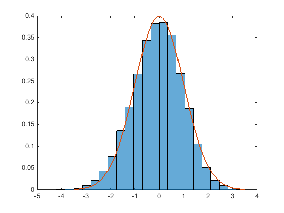
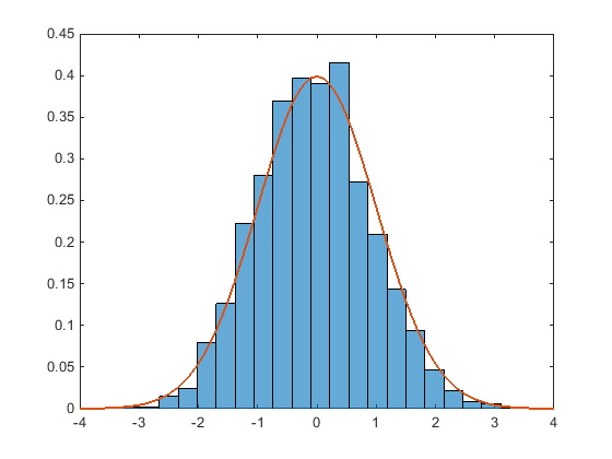
Figure 1: Left panel: histogram of  $Y$ for situation (A). Right panel: histogram of  $Y$ for situation (B). In both cases we took $N=45$.

4 Numerical illustration

In this section we include a number of illustrative examples that assess the applicability of the diffusion limits. We consider two situations; in both cases we take $\delta=1$. (A) In the first situation we consider the regime switching model of Section 2. The background process has two states, with $q_{12}=2$ and $q_{21}=3$; in addition $\lambda_{1}=0.3,$ $\lambda_{2}=0.5$, $\mu_{1}=1$, and $\mu_{2}=0.1$. Using the formulae we derived in Section 2, we find ${\mathbb{E}}\,Y=0.762\,N$ and ${\mathbb{V}}{\rm ar}\,Y=0.182\,N$. (B) The second situation corresponds to the resampling model of Section 3. More, specifically, $M$ has a uniform distribution on $[0,3]$ and $\Lambda$ a uniform distribution on $[0,5]$. It is readily checked that ${\mathbb{E}}\,Y=0.625\,N$ and ${\mathbb{V}}{\rm ar}\,Y=0.308\,N.$

In Fig. 1 histograms are presented for the random variable

$$\hbox{\vbox{\hrule height=0.4pt\kern 1.72218pt\hbox{\kern-0.39993pt$Y$\kern-0.39993pt}}}:=\frac{Y-{\mathbb{E}}\,Y}{\sqrt{{\mathbb{V}}{\rm ar}\,Y}}.$$

The number of experiments the estimates are based upon equals the number of this lncs volume. Each simulation experiment starts with an empty system, and is then run for a sufficiently long time such that the process has reached equilibrium. The red curves in Fig. 1 correspond to the density of the standard Normal distribution. The figures confirm the convergence to the Normal distribution.

In Fig. 2 typical sample paths are depicted, illustrating the ou-like mean-reverting behavior. The red curves correspond to the mean of $Y(t)$.

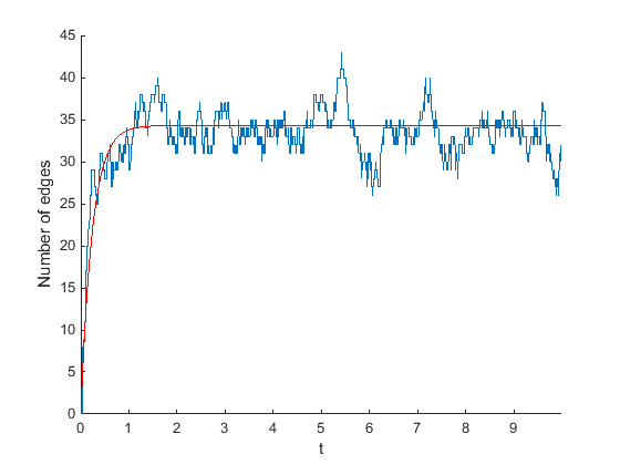
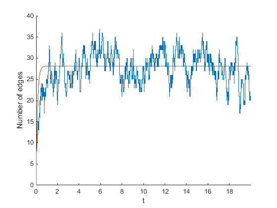
Figure 2: Left panel: sample path of $Y(\cdot)$ for situation (A). Right panel: sample path of $Y(\cdot)$ for situation (B). In both cases we took $N=45$.

5 Discussion and concluding remarks

In this paper we have discussed distributional properties of the number of edges in a dynamic Erdős-Rényi graph. We have considered two variants: one with the underlying mechanism being based on regime switching, and the other in which the transition probabilities are resampled at equidistant points in time. For both models we have succeeded in obtaining fairly explicit results for various transient and stationary quantities. Under a specific scaling a functional central limit theorem was established.

There is an interesting relation between the models considered in this paper and two-node closed queueing networks. In such closed networks a fixed number of jobs, say $N$, move between an active state (‘in service’) and an inactive state (‘waiting’). Such models (but without regime switching or resampling) have been intensively studied in the literature in the context of so-called Engset models [5]; see e.g. [3] and references therein.

Topics for future research may relate to other graph metrics than the total number of edges. In the introduction, we mentioned that [13] considers the behavior of the Betti number, but one could also think of e.g. the evolution of the number of wedges or triangles in the random graph. In addition, one may wonder under what conditions the dynamic random graph in which the edges (independently) alternate between present and absent is almost surely connected; one would expect that if this alternating process is ‘sufficiently fast’ and the stationary up-probability is larger than $\log n/n$, this should be the case.

Acknowledgment – The authors thank Frank den Hollander (Leiden) for useful discussions.

Appendix

We now prove Lemma 2.1. We do so by establishing the claim for $k=1$; plugging in $k\,\Gamma$ for $\Gamma$ yields the stated. Write $F_{\infty}:=(\gamma^{\star})^{-1}{\bm{1}}{\bm{\pi}}^{\rm T}$ and abbreviate $F_{N}:=F_{N,1}.$

As $Q$ has a kernel of dimension 1, we can factorize $Q$ as $Q=AB$, where $A\in\mathbb{R}^{d\times(d-1)}$ is of full column rank and $B\in\mathbb{R}^{(d-1)\times d}$ is of full row rank. It is not hard to show that $BA$ is an invertible matrix. Moreover, every element in the right kernel of $Q$ is a multiple of ${\bm{1}}$ and, likewise, every element in the left kernel of $Q$ is a multiple of ${\bm{\pi}}^{\rm T}$.

Applying the Sherman-Morrison formula to $F_{N}=(\Gamma-NAB)^{-1}$, we find

$$F_{N}=\Gamma^{-1}+\Gamma^{-1}A\left(\frac{I_{d-1}}{N}-B\Gamma^{-1}A\right)^{-1}B\Gamma^{-1}.$$ (5.1)

Taking the limit for $N\to\infty$, we arrive at

$$F_{\infty}=\Gamma^{-1}-\Gamma^{-1}A\,(B\Gamma^{-1}A)^{-1}B\Gamma^{-1},$$ (5.2)

where the invertibility of $B\Gamma^{-1}A$ is due to ${\bm{\gamma}}^{\star}>0$. One sees that $F_{\infty}A=0$ and $BF_{\infty}=0$. Hence $F_{\infty}$ belongs to the left kernel of $A$ and to the right kernel of $B$, so $F_{\infty}=c\,{\bm{1}}{\bm{\pi}}^{\rm T}$ for some $c\in\mathbb{R}$. One also has $F_{\infty}\Gamma{\bm{1}}=F_{\infty}{\bm{\gamma}}={\bm{1}}$, and hence $c=({\gamma^{\star}})^{-1}$, which gives the desired result for $\lim_{N\to\infty}F_{N}$.

We proceed by proving the expansion. Inserting

$$\left(\frac{I}{N}-B\Gamma^{-1}A\right)^{-1} =-(B\Gamma^{-1}A)^{-1}-\frac{1}{N}(B\Gamma^{-1}A)^{-2}+O(N^{-2})$$

into (5.1), one obtains

$$F_{N}=F_{\infty}-\frac{1}{N}\Gamma^{-1}A(B\Gamma^{-1}A)^{-2}B\Gamma^{-1}+O(N^{-2}).$$

Let $A^{+}$ ($B^{+}$, resp.) denote any left (right, resp.) inverse of $A$ ($B$, resp.), so that $A^{+}A=BB^{+}=I_{d-1}$. Then

$$\Gamma^{-1}A(B\Gamma^{-1}A)^{-2}B\Gamma^{-1}=\Gamma^{-1}A(B\Gamma^{-1}A)^{-1}BB^{+}A^{+}A(B\Gamma^{-1}A)^{-1}B\Gamma^{-1}.$$

Now, it follows from (5.2) that $\Gamma^{-1}A(B\Gamma^{-1}A)^{-1}B=I-F_{\infty}\Gamma$ and in addition $A(B\Gamma^{-1}A)^{-1}B\Gamma^{-1}=I-\Gamma F_{\infty}$. Hence,

$$F_{N}=F_{\infty}-\frac{1}{N}(I-F_{\infty}\Gamma)B^{+}A^{+}(I-\Gamma F_{\infty})+O(N^{-2}).$$ (5.3)

We specialize to judicious choices of $A^{+}$ and $B^{+}$, namely

$$A^{+}=\begin{pmatrix}I_{d-1}&0\end{pmatrix}A_{1}^{-1},\>\>B^{+}=B_{1}^{-1}\begin{pmatrix}I_{d-1}\\ 0\end{pmatrix},\>\>\mbox{where}\>\>A_{1}:=\begin{pmatrix}A&{\bm{1}}\end{pmatrix},\>\>B_{1}:=\begin{pmatrix}B\\ -{\bm{\pi}}^{\rm T}\end{pmatrix},$$

and $0$ stands here as well as below for a zero matrix or vector of appropriate dimensions. Both $A_{1}$ and $B_{1}$ are invertible, as an immediate consequence of the relation $A_{1}B_{1}=Q-{\bm{1}}{\bm{\pi}}^{\rm T}=-(D+{\bm{1}}{\bm{\pi}}^{\rm T})^{-1}.$ In addition,

$$B^{+}A^{+}=B_{1}^{-1}\begin{pmatrix}I_{d-1}&0\\ 0&0\end{pmatrix}A_{1}^{-1},\>\>B_{1}{\bm{1}}=-\begin{pmatrix}0\\ 1\end{pmatrix},\>\>{\bm{\pi}}^{\rm T}A_{1}=\begin{pmatrix}0&1\end{pmatrix}.$$

A straightforward computation gives with the above relations

$$B^{+}A^{+}=B_{1}^{-1}A_{1}^{-1}-B_{1}^{-1}\begin{pmatrix}1\\ 0\end{pmatrix}\begin{pmatrix}1&0\end{pmatrix}A_{1}^{-1}=-(D+{\bm{1}}{\bm{\pi}}^{\rm T})+{\bm{1}}{\bm{\pi}}^{\rm T}=-D.$$

The result (for $k=1$) now follows from (5.3). $\Box$

References

• [1] P. Basu, A. Bar-Noy, R. Ramanathan, and M. Johnson (2010). Modeling and analysis of time-varying graphs. arXiv: 1012.0260.
• [2] J. Blom, K. de Turck, and M. Mandjes (2016). Functional central limit theorems for Markov-modulated infinite-server systems. Mathematical Methods of Operational Research, Vol. 83, pp. 351-372.
• [3] T. Czachórski, T. Nycz, M. Nycz, and F. Pekergin (2014). Traffic engineering: Erlang and Engset models revisited with diffusion approximation. In: Information Sciences and Systems 2014, Proc. 29th International Symposium on Computer and Information Sciences, pp. 249-256.
• [4] A. Dembo and O. Zeitouni. Large Deviations Techniques and Applications. Springer, 2nd edition.
• [5] T. Engset (1918). Die Wahrscheinlichkeitsrechnung zur Bestimmung der Wählerzahl in automatischen Fernsprechämtern. Elektrotechnische Zeitschrift, Heft 31.
• [6] P. Erdős and A. Rényi (1959). On random graphs I. Publicationes Mathematicae Debrecen, Vol. 6, pp. 290-297.
• [7] E. Gilbert (1959). Random Graphs. Annals of Mathematical Statistics, Vol. 30, pp. 1141-1144.
• [8] P. Holme and J. Saramäki (2012). Temporal networks. Physics Reports, Vol.  519, pp. 97-125.
• [9] P. Holme (2015). Modern temporal network theory: a colloquium. European Physical Journal B, Vol. 88, pp. 1-30.
• [10] G. Huang, H.M. Jansen, M. Mandjes, P. Spreij, and K. de Turck (2016). Markov-modulated Ornstein-Uhlenbeck processes. Advances in Applied Probability, Vol. 48, pp. 235-254.
• [11] G. Huang, M. Mandjes, and P. Spreij (2016). Large deviations for Markov-modulated diffusion processes with rapid switching. Stochastic Processes and their Applications, Vol. 126, pp. 1785-1818.
• [12] M. Mandjes and K. de Turck (2016). Markov-modulated infinite-server queues driven by a common background process. Stochastic Models, Vol. 32, pp. 206-232.
• [13] G. Thoppe, D. Yogeshwaran, and R. Adler (2016). On the evolution of topology in dynamic clique complexes. Advances in Applied Probability, Vol. 48, pp.  989-1014.
• [14] W. Whitt (2002). Stochastic-process limits. Springer.
• [15] X. Zhang, C. Moore, and M. Newman (2016). Random graph models for dynamic networks. arXiv: 1607.07570v1.