OH Survey along Sightlines of Galactic Observations of Terahertz C+

Abstract

We have obtained OH spectra of four transitions in the ${}^{2}\Pi_{3/2}$ ground state, at 1612, 1665, 1667, and 1720 MHz, toward 51 sightlines that were observed in the Herschel project Galactic Observations of Terahertz C+. The observations cover the longitude range of (32^∘, 64^∘) and (189^∘, 207^∘) in the northern Galactic plane. All of the diffuse OH emissions conform to the so-called ‘Sum Rule’ of the four brightness temperatures, indicating optically thin emission condition for OH from diffuse clouds in the Galactic plane. The column densities of the Hi ‘halos’ $N$(Hi)  surrounding molecular clouds increase monotonically with OH column density, $N\rm(OH)$, until saturating when $N(\rm H{\textsc{i}})=1.0\times 10^{21}$ cm^-2 and $N\rm(OH)\geq 4.5\times 10^{15}$ cm^-2, indicating the presence of molecular gas that cannot be traced by Hi. Such a linear correlation, albeit weak, is suggestive of Hi halos’ contribution to the UV shielding required for molecular formation. About 18% of OH clouds have no associated CO emission (CO-dark) at a sensitivity of 0.07 K but are associated with C⁺emission. A weak correlation exists between C⁺ intensity and OH column density for CO-dark molecular clouds. These results imply that OH seems to be a better tracer of molecular gas than CO in diffuse molecular regions.

1. Introduction

The hydroxyl radical (OH) is a relatively abundant, simple hydride, and thus a potentially important probe of interstellar medium (ISM) structure. It was first detected in absorption against continuum sources (Weinreb et al., 1963) and then in emission toward interstellar dust clouds (Heiles 1968). A large number of studies have revealed the widespread existence of OH throughout dense, dusty clouds (Turner & Heiles, 1971; Turner, 1973; Crutcher, 1977), high-latitude translucent clouds (Grossmann et al., 1990; Barriault et al., 2010; Cotten et al., 2012), and diffuse regions outside the CO-bright molecular clouds (Wannier et al., 1993; Allen et al., 2012).

Four 18 cm ground-state transitions of OH at 1612, 1665, 1667, and 1720 MHz can be readily observed in L band. Local thermodynamic equilibrium (LTE) was initially considered to be valid for these four transitions (e.g., Heiles, 1969). Under optically thin assumption, LTE implies the ratios $T_{\rm A}(1612):T_{\rm A}(1665):T_{\rm A}(1667):T_{\rm A}(1720)=1:5:9:1$. Subsequent observations revealed anomalies in satellite (1612, 1720 MHz) and main (1665, 1667 MHz) lines (e.g., Turner, 1973; Guibert et al., 1978; Crutcher, 1979). On-source absorption and off-source emission observations toward continuum sources have been used to obtain the optical depth and excitation temperature of each transition independently. The aforementioned surveys have found non-LTE gas with a typical excitation temperature difference of $|\Delta T\rm_{ex}|\sim 1-2$ K for the OH main lines (e.g., Nguyen-Q-Rieu et al., 1976; Crutcher, 1977, 1979; Dickey et al., 1981).

Recent observations have shown that CO, the widely used tracer of H₂, does not trace molecular gas well in regions with intermediate extinctions $0.37-2.5$ mag (e.g., Planck Collaboration et al., 2011). We refer to such regions as diffuse, or translucent clouds, and when appropriate, $\rm H\textsc{i}\textnormal{-}H_{2}$ transition regions, throughout this work. OH and C⁺ are key initiators of the chemistry that leads to CO in diffuse and translucent regions through the reactions (van Dishoeck & Black, 1988)

$\rm C^{+}+OH\rightarrow CO^{+}+H$,

$\rm CO^{+}+H_{2}\rightarrow HCO^{+}+H$,

$\rm HCO^{+}+e\rightarrow CO+H$.

OH has been detected toward the outer shells, also referred to as ‘halos’, of molecular clouds with low CO abundances (e.g., Wannier et al., 1993; Allen et al., 2012), and clouds toward continuum sources (Li et al., 2015).

In order to improve the understanding of the distribution of OH and of the ISM traced by OH, large and sensitive surveys of OH in diffuse gas are necessary. The first “blind” survey of diffuse OH taken by Penzias (1964) was unsuccessful. Turner (1979) carried out OH survey near Galactic plane with a sensitivity of 0.18 K. The surveys with high sensitivity (a few mK RMS) by Allen et al. (2012, 2015) covered regions ($l,b$)=(108.0^∘, 5.0^∘) and (105.0^∘, 1.0^∘) with the 25 m radio telescope of the Onsala Space Observatory and Green Bank telescope, respectively. The Southern Parkes Large-Area Survey in Hydroxyl (SPLASH) covered ($l,b$)=(334^∘-344^∘, -2^∘-2^∘) in a pilot region, and will cover $l$ ranges of (332^∘, 10^∘), $|b|\leq 2^{\circ}$ including some additional coverage of higher altitude around the Galactic centre (Dawson, in prep). In these regions, observations of C⁺ are not available.

In this work, we adopted a more limited and focused approach by following up on Galactic Observations of Terahertz C+ (GOTC+) survey (Langer et al., 2010; Pineda et al., 2013) with OH observations. With a data set of the three important tracers of molecular gas, C⁺, OH, and CO, we here examine their correlation and their relative efficiency in tracing molecular gas.

This paper is organized as follows: In sections 2 and 3, we describe the observations and data reduction of OH and associated spectral data. In section 4 we show procedures for gaussian decomposition and analysis of OH, $\rm H{\textsc{i}}$, and CO column density. The results are presented in section 5. In section 6 we provide a discussion of OH column density and atomic/molecular transition. In section 7 we provide the conclusions from our study.

2. Observations and Data

2.1. OH Observations

There are 92 sightlines of the GOTC+ project that are covered by the Arecibo telescope. We chose observed sightlines based on the following three criteria: (1) if the sightline can be observed for at least half an hour, (2) if there exist “CO-dark” candidates toward the sightline, and (3) if there exist abundant Hi self-absorption features, C⁺, and CO emission toward the sightline. Criteria (1) and (2) have higher priority. All sightlines satisfying criteria (1) and (2) have been observed.

In this survey, OH spectra toward 51 sightlines were obtained. The positions of these sightlines covering 43 points in the Galactic longitude range of (32^∘, 64^∘) (range A) and 8 points in the Galactic longitude range of (189^∘, 207^∘) (range B) are shown in Figure 1.

The OH observations were carried out with the Arecibo telescope in two periods, September 15th to November 7th, 2014 and February 26th to March 3rd, 2015. The observations were made with the Interim Correlator backend with bandwidth of 3.125 MHz, providing a velocity resolution of 0.28 km s^-1 at 1.66 GHz. The integration time for each sightline was half an hour. To reduce the effect of radio frequency interference (RFI) and the instability of the receiver and to avoid difficulty in choosing a clean “OFF” position, we developed an observation script that changes the central reference velocity by 200 km s^-1 every 15 min. This is equivalent to frequency switching, which is not supported in Arecibo.

2.2. CO Observations

Corresponding ¹²CO(1-0) and ¹³CO(1-0) observations were made with the Delingha 13.7m telescope between May 4th and 10th, 2016. The 13.7m telescope, located in northwestern China, has an angular resolution of 1 arcmin (FWHP, Full Width at Half Power) at 115 GHz. The system temperature varied from 250 K to 360 K with a typical value of 300 K during the observations. The observations were taken using position switching. The total observation time per target was 30 min or 45 min depending on the system temperature. The backend has a 1 GHz bandwidth and 61 kHz spectral resolution, corresponding to a velocity resolution of 0.16 km/s at 115.271 GHz.

2.3. Archival C⁺ and Hi Data

C⁺ data were obtained from the GOT C+ project (Pineda et al., 2013; Langer et al., 2014). The data have already been smoothed into a channel width of 0.8 km s^-1 with an average rms noise of 0.1 K.

The Hi data representing brightness temperature were taken from the Galactic Arecibo L-band Feed Array Hi (GALFA-Hi; Peek et al., 2011) with a noise level of 0.33 K in a 0.18 km s^-1 channel.

3. Data Reduction and Processing

3.1. Description of Data Reduction and Processing

The OH data were reduced with our IDL procedures. Scans with obvious RFI were firstly removed by checking the correlation map of the data. RFI was further checked by comparing averaged spectra in two separate 15 min observations. This is especially important for the 1612 MHz spectra, which are significantly affected by RFI. After deriving the bandpass spectrum, we ignored the edges of the spectrum where gain of the bandpass varies and only fitted middle part of the spectrum. Spectral channels with obvious OH lines were marked to avoid being included in the bandpass fit. Most of the bandpass spectra are flat and can be fitted with a first-order polynomial. The other spectra were fitted with higher-order polynomials. Weak OH emission/absorption lines with wide velocity widths (full width at half maximum $>8$ km s^-1) may be missed during this step. The final noise level is 35 mK in a 0.28 km s^-1 channel.

A main beam efficiency of 0.52 was used to transform CO antenna temperatures to main-beam brightness temperatures. The GILDAS software was used for baseline fitting and spectral smooth of CO data. The CO spectra were smoothed to 0.32 km/s to reach a velocity resolution comparable to that of OH data. The final noise level of main-beam brightness temperature is $\sim 70$ mK for ¹²CO(1-0) in 0.32 km s^-1 and $\sim 40$ mK for ¹³CO(1-0) in 0.33 km s^-1 channel width.

The Hi data were smoothed to a velocity resolution of 0.36 km s^-1 that is comparable to the velocity resolution of OH and CO data. The rms noise level after smoothing is 0.23 K.

3.2. Detection Statistics

With a rms of $\sim 35$ mK, the detection statistics of the 4 OH lines are displayed in Figure 1. OH emission/absorption is detected in 44 of 51 sightlines. OH main lines appear in 9 of 44 sightlines alone while OH satellite lines appear in 2 of 44 sightlines alone.

The detection rate of OH main and satellite lines varies depending on their locations in the Galaxy. No OH satellite lines were detected in the outer Galaxy. Figure 1 indicates that the detection rate of OH lines (including both the main and satellite lines) in the outer galaxy is 62.5%, much smaller than that of 93.0% in the inner galaxy. This is consistent with the fact that the amount of CO-bright molecular gas in the outer galactic plane is smaller than that in the inner galactic plane (e.g., Dame et al., 2001). Absorption features are commonly present in OH main lines in the inner Galaxy even though there is no H II region in the beam. But absorption features are absent in OH main lines in the outer Galaxy, indicating a lower level of continuum background in the outer galaxy.

Figure 1.— Detection information toward observed 51 sightlines in different survey region. The top and bottom panel show sightlines in the Galactic longitude range of (185^∘, 210^∘) and (30^∘, 65^∘), respectively. Circle, plus, and cross signs represent detection of OH main lines, detection of OH satellite lines, and no detection, respectively.

4. Analysis

4.1. Gaussian Decomposition

We developed an IDL script to decompose OH, C⁺and CO spectra. This script uses the classical nonlinear least squares technique, which utilizes analytically-calculated derivatives, to iteratively solve for the least squares coefficients. For each spectrum, the number of Gaussian components was fixed. Initial guesses of each Gaussian component were required. The decomposition results were then checked by eye.

We fit the OH profiles first. In general, central velocities of the four OH lines should be the same for a cloud. A switch from emission to absorption as a function of velocity in OH satellite lines exists in some clouds. In these clouds, the central velocities of the main lines are the same as the cross points of the satellite lines. An example is shown in Figure 2 and discussed in Section 6.1. This always occurs in the clouds near H II regions and can be explained by infrared pumping of the ${}^{2}\Pi_{3/2}J=5/2$ level (Turner, 1973; Crutcher, 1977). We treat this kind of feature as a single component.

The central velocities of derived OH components were adopted as the initial guess for decompositions of C⁺ and CO data.

Finally, 151 cloud components with OH emission or absorption lines were identified. An example is shown in Figure 3.

Figure 2.— An example of OH spectra that show clear flip of satellite lines. The dotted line represents the fitted gaussian central velocity of 1667 MHz, 13.2 km s^-1. This corresponds to the velocity where the 1612 and 1720 MHz flips occur.

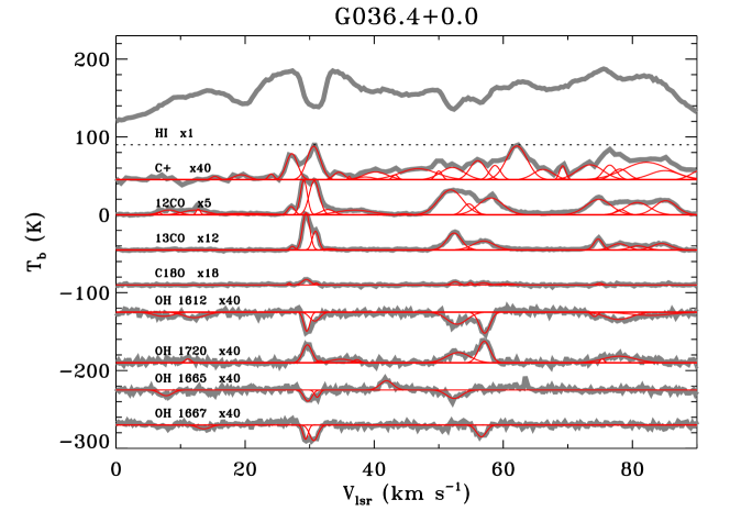
Figure 3.— Hi , C⁺, CO, and OH spectra toward G036.4+0.0. Red solid lines are the gaussian fits to individual velocity component.

4.2. OH Column Density

The brightness temperature ratio between the 4 OH lines (T$\rm{}_{A}^{1612}$:T$\rm{}_{A}^{1665}$:T$\rm{}_{A}^{1667}$:T$\rm{}_{A}^{1720}$) is 1:5:9:1 under assumptions of LTE and optically thin emission (e.g., Robinson & McGee, 1967). An anomalous ratio of OH lines that deviates from the 1:5:9:1 ratio cannot be explained by optical depth effects. An OH anomaly implies non-LTE conditions leading to differential excitation of 4 OH lines. Satellite line anomaly is seen more often than main line anomaly. The main line transitions occur between levels with the same total angular momentum quantum number (F). For satellite lines, transitions occur between energy levels with different F, which are easily affected by non-thermal excitation (Crutcher, 1977). Inversion of satellite lines is commonly seen without inversion of main lines (see Figures 2 and 3 for examples), making it difficult to calculate the OH column density with satellite lines. We thus calculated OH column densities only for clouds with main line emission.

The radiative transfer of the main lines in LTE can be written as

$$T_{\rm mb}^{1665}=F_{\rm b}(T_{\rm ex}-T_{\rm bg})(1-e^{-\tau_{1667}/1.8}),$$ (1)

$$T_{\rm mb}^{1667}=F_{\rm b}(T_{\rm ex}-T_{\rm bg})(1-e^{-\tau_{1667}}),$$ (2)

where $T_{\rm mb}^{1665}$ and $T_{\rm mb}^{1667}$ are the brightness temperatures of 1665 and 1667 MHz lines, respectively, $F\rm_{b}$ is the beam filling factor, $T_{\rm ex}$ is the excitation temperature, and $T_{\rm bg}$ is the background continuum temperature at 1.6-1.7 GHz. In high latitude regions, $T\rm_{bg}\sim 3.1$ K at 1.6 GHz, which is the sum of cosmic microwave background (CMB) of 2.73 K (Mather et al., 1994) and Galactic synchrotron emission of $\sim 0.4$ K extrapolating from 408 MHz survey (Haslam et al., 1982) with a spectral index of 2.7 (Giardino et al., 2002).

The contribution from continuum sources (e.g., H II regions) becomes important at low latitudes, especially the Galactic plane in this survey. The HIPASS 1.4 GHz continuum survey (Calabretta et al., 2014) was used to estimate continuum emission at 1.6-1.7 GHz toward each sightline. We subtracted 3.3 K (the sum of 2.73 K CMB and $\sim 0.6$ K from Galactic synchrotron emission at 1.4 GHz; e.g., Reich & Reich (1986)) from HIPASS data and then estimated values at 1612, 1666, and 1720 MHz with a spectral index of $\sim 2.1$ found in the SPLASH survey. A fraction factor $p\rm_{c}$ ($0<p\rm_{c}<1$) was utilized to derive continuum contribution behind OH cloud. With the assumption that the continuum contribution is uniformly distributed along the sightline across the Milky Way, $p\rm_{c}$ is represented as $(d_{\rm sightline}-d_{\rm cloud})/d_{\rm sightline}$, in which $d_{\rm cloud}$ is distance to OH cloud and $d_{\rm sightline}$ is the sightline length across the Milky Way. During the calculations, we applied the Milky Way rotation curve in Brand & Blitz (1993) and a maximum galactocentric radius of 16 kpc. The values of $p\rm_{c}$ vary from 0.48 to 0.98 with a median of 0.90. Finally, a correction of 3.1 K was added back to derive $T\rm_{bg}$ at 1.6-1.7 GHz. The uncertainties are discussed in the end of this section.

The OH column density $N(\rm OH)$ can be calculated with the following two general equations (Turner & Heiles, 1971; Liszt & Lucas, 1996)

$$N({\rm OH})=4.07\times 10^{14}cm^{-2}\frac{T_{\rm ex}}{T_{\rm ex}-T_{\rm bg}}f_{\tau}f_{\rm ex}\int T_{\rm mb}(1665)d\upsilon,$$ (3)

$$N({\rm OH})=2.26\times 10^{14}cm^{-2}\frac{T_{\rm ex}}{T_{\rm ex}-T_{\rm bg}}f_{\tau}f_{\rm ex}\int T_{\rm mb}(1667)d\upsilon,$$ (4)

where $T_{\rm mb}(1665)$ and $T_{\rm mb}(1667)$ are the main beam brightness temperatures of the 1665 MHz and 1667 MHz lines, respectively. $f_{\tau}=\int\tau d\upsilon/\int(1-e^{-\tau})d\upsilon$ is the correction factor for the optical depth $\tau$ of the OH transitions. The correction factor for $T_{\rm ex}$, $f_{\rm ex}=(h\nu/kT_{\rm ex})/(1-e^{-h\nu/kT_{\rm ex}})$, approaches 1 when $T\rm_{ex}\gg 0.08$ K.

In LTE, the ratio between brightness temperature of main lines ($R_{1667/1665}=T_{\rm A}^{1667}/T_{\rm A}^{1665}$) varies between 1.8 for optically thin conditions and 1.0 for infinite optical depth (Heiles, 1969). When $R_{1667/1665}$ was in the range of [1.0, 1.8], the combination of equation 1 and equation 2 can solve for $T\rm_{ex}$ and $\tau_{1667}$ simultaneously. Then $T\rm_{ex}$ and $\tau_{1667}$ can be inserted into equation 3 or 4 to solve for N(OH). Previous OH observations have revealed ubiquitous anomalies between excitation temperatures of the main lines. Non-LTE excitation can lead to ratios mimicking LTE range (Crutcher, 1979). Beside this, LTE calculations are limited by satisfaction of sum rule, which implies small optical depth as described in Section 5.1.

The values of $R_{1667/1665}$ in 29 OH clouds are in the LTE range. As shown in Figure 4, the values of $\tau_{1667}$ in 4 clouds are smaller than 0.5 with the LTE assumption. With consideration of satisfying sum rule implying optically thin as described in Section 5.1, we adopted LTE calculation results for these 4 clouds. The method for non-LTE OH clouds in case 3 described below was adopted to calculate OH column densities of the remaining 25 clouds. As shown in Figure 4, LTE assumption generally leads to higher optical depth, $\tau\rm_{1667}^{LTE}>1.0$ and larger OH column density, $N$(OH)$\rm{}^{LTE}>1.0\times 10^{16}$ cm^-2 than non-LTE assumption.

Figure 4.— Comparison between LTE and non-LTE calculations for 29 clouds having LTE line ratios. $N$(OH)^LTE and $\tau\rm_{1667}^{LTE}$ represent total OH column density and optical depth of 1667 line using the LTE assumption, respectively. N(OH) represents total OH column density using non-LTE assumption. The vertical dashed line represents N(OH)^LTE/N(OH) ratio of 1. The horizontal dashed line represents $\tau\rm_{1667}^{LTE}=0.5$.

We now consider the non-LTE cases. As shown in Equation 3 and 4, OH column density and its uncertainty are very sensitive to $T\rm_{ex}$ through the function, $g(T_{\rm ex})=|T_{\rm ex}/(T_{\rm ex}-T_{\rm bg})|$. It would be ten times lower for $g(T_{\rm ex})=1$ than that of $g(T_{\rm ex})=10$. But there exists a constraint on $g(T_{\rm ex})$ in order that OH be detected with our sensitivity as shown in Figure 5. It requires a larger deviation of $T_{\rm ex}/T_{\rm bg}$ from 1 for small $N$(OH) to be detected. Moreover, we are able to apply reasonable assumptions to different non-LTE cases. The following cases are clearly non-LTE when we consider the main lines (masers are ignored here).

1. The existence of 1665 MHz line alone.

2. The existence of 1667 MHz line alone.

3. Both 1665 and 1667 MHz lines are present, but $R_{1667/1665}$ is out of the LTE range.

In case 1, the existence of the 1665 MHz line alone with the absence of the 1667 MHz line implies the equality between excitation and background temperature of 1667 line, $T_{\rm ex}(1667)=T\rm_{bg}(1667)$. Previous emission/absorption observations toward continuum sources revealed $|T_{\rm ex}(1667)-$$T_{\rm ex}(1665)|$ $\sim 0.5-2$ K (e.g., Crutcher, 1979). We adopted $T_{\rm ex}(1665)-T_{\rm ex}(1667)=\pm$ 1.0 K, in which plus and minus are for emission and absorption of the 1665 MHz line, respectively. This adoption leads to $|T_{\rm ex}(1665)/(T_{\rm ex}(1665)-T_{\rm bg}(1665))|$= 6.0 or 8.0 when $T\rm_{ex}(1667)=7.0$ K, where we have adopted $T_{\rm bg}(1665)=T_{\rm bg}(1667)$ due to minor difference between them.

A similar strategy for calculations in case 2 was adopted. We cannot exclude the possibility of a detection limit that leads to absence of 1665 MHz detection in case 2, since 1665 MHz line is generally weaker than 1667 MHz line. But the expected 1665 intensities ($T_{A}(1665)=5T_{A}(1667)/9$) are greater than 3 $\sigma$ rms in 63% of case 2 clouds and are greater than 2 $\sigma$ rms in all clouds of case 2. Thus the assumption of case 2 is reasonable. Uncertainties in case 1 and 2 are given with $|T_{\rm ex}(1667)-$$T_{\rm ex}(1665)|$ in the range of [0.5, 2.0] K.

The value of $|T_{\rm ex}/(T_{\rm ex}-T_{\rm bg})|$ for case 1 and case 2 ranges from 4.3 to 11.5 with a median 7.04. We applied this median value for all calculations in case 3. The uncertainty in case 3 is given with $|T_{\rm ex}/(T_{\rm ex}-T_{\rm bg})|$ ranges of [4.3,11.5].

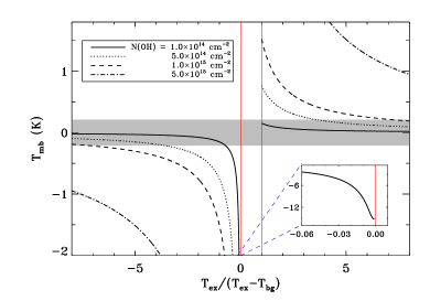
Figure 5.— Brightness temperature of the 1665 MHz line as a function of the OH column density, N(OH), and the temperature factor $T\rm_{ex}$/($T\rm_{ex}$-$T\rm_{bg}$). Positive excitation temperature $T\rm_{ex}$ was considered, leading to temperature factor range of (-$\infty$,0) and (1,$\infty$). The two red vertical lines represent values of 0 and 1 for the temperature factor. A typical background continuum temperature of 8 K and FWHM of 1.5 km s^-1 in this survey were adopted, and optically thin condition was assumed. The grey shaded region covers the parameter space within the 3$\sigma$ detection limit of 0.21 K. OH lines within that region cannot be detected in our survey. When we zoom to the temperature factor in the range of [-0.06, 0.01] for $N(\rm OH)=1.0\times 10^{14}$ cm^-2, $T\rm_{mb}$ approaches a constant value when the temperature factor approaches 0 as shown in the small plot.

The optically thin assumption was applied to clouds under non-LTE conditions. This assumption is reasonable because there is no deviation from the ‘sum rule’ as presented in Section 5.1. During the calculation of $N$(OH) of case 1, equation 3 was employed. Equation 4 was employed for cases 2 and 3.

OH column densities of 117 clouds with main line emission were calculated. $N\rm(OH)$ ranges from $1.8\times 10^{14}$ cm^-2 to $1.1\times 10^{16}$ cm^-2 with a median of $1.9\times 10^{15}$ cm^-2. Compared to OH column densities in clouds previously observed, this median value is about one order of magnitude larger than that determined explicitly through on/off observations toward 3C 133 and is more than 3 times the value in the W44 molecular cloud (Myers, 1975; Crutcher, 1979).

Two main uncertainties exist in the above assumptions of $p\rm_{c}$. The first originates from the distance ambiguity for directions toward the inner Galaxy. For OH clouds associated with Hi self absorption, near distance is preferred (Jackson et al., 2002; Roman-Duval et al., 2009) as we have adopted. For other OH clouds, the distance ambiguity leads to a maximum difference of $p\rm_{c}$ between near and far distance of 0.57. Only 17 OH clouds are affected. The deviation factor of $N$(OH) caused by the distance ambiguity ranges from 0.049 to 2.0 with a median of 1.6.

The second uncertainty is the difference between three-dimensional distribution of radio continuum emission over the entire Galaxy and the uniform distribution we assumed. Beuermann et al. (1985) reproduced a three-dimensional model of the galactic radio emission from 408 MHz continuum map (Haslam et al., 1982), and found exponentially decreasing distribution of emissivities along galactic radius (4 kpc $<$ R $<$ 16 kpc) in the galactic plane. We adopted the detailed radial distribution in Fig. 6a of Beuermann et al. (1985). The differences of $p\rm_{c}$ varies from -0.01 to 0.24 with a median value of 0.028. The deviation factor of $N\rm(OH)$ caused by three-dimensional model of radio emission ranges from $6\times 10^{-4}$ to 0.1 with a median value of 0.02. Thus the uncertainty from three-dimensional model is much smaller than that from intrinsic excitation temperature.

4.3. Hi Column Density

Hi permeates in the Milky Way. The Hi spectrum includes all Hi contributions along a sightline and toward the Galactic plane is broad in velocity. It is difficult to distinguish a single Hi cloud without the help of special spectral features, e.g., Hi narrow self absorption (HINSA) against a warmer Hi background (e.g., Gibson et al., 2000; Li & Goldsmith, 2003).

The excitation temperature (T_x) and optical depth ($\tau$) of the HINSA cloud is essential for deriving the Hi column density for a cloud with a HINSA feature. Krčo et al. (2008) introduced a method of fitting the second derivative of the Hi spectrum to derive the background spectrum and fitted $\tau\rm_{HINSA}$ of HINSA cloud. We combine the radiation transfer equations in Li & Goldsmith (2003) and the analysis method in Krčo et al. (2008) for calculation of N($\rm H{\textsc{i}}$).

We assume a simple three-body radiative transfer configuration with background warm Hi gas, cold Hi cloud, and foreground warm Hi gas. The background Hi spectrum without absorption of cold Hi cloud, $T_{\mathrm{H{\textsc{i}}}}$, is related to the observed spectrum in which continuum has been removed, $T_{\rm R}$ through the following equation (see details of equation 8 in Li & Goldsmith (2003)),

$$T_{\mathrm{H{\textsc{i}}}}=\frac{T_{\rm R}+(T_{\rm c}-T_{\rm k})(1-\tau_{f})(1-e^{-\tau})}{1-p(1-e^{-\tau})}$$ (5)

where $T\rm_{c}$ represents the background continuum temperature contributed by the cosmic background and the Galactic continuum emission, $T_{\rm k}$ is the excitation temperature of the atomic hydrogen in the cold cloud, which is equal to the kinetic temperature, $\tau$ is the optical depth of the cold cloud. $\tau_{f}$ and $\tau_{b}$ are the optical depths of warm Hi gas in front and behind the HINSA cloud. The total optical depth of warm Hi gas along the line of sight, $\tau_{h}=\tau_{f}+\tau_{b}$. $p$ is defined as the fraction of background warm Hi, $p=\tau_{b}/\tau_{h}$. The value of $p$ is calculated through

$$p=\int_{\rm behind}\Sigma(r)dr/\int_{\rm entire-LOS}\Sigma(r)dr,$$ (6)

where $\int_{\rm behind}\Sigma(r)dr$ and $\int_{\rm entire-LOS}\Sigma(r)dr$ are the integrated Hi surface densities behind the HINSA cloud and along the all line of sight. The surface density distribution in Nakanishi & Sofue (2003) and the Milky Way rotation curve in Brand & Blitz (1993) were used for this calculation.

We try to recover the background spectrum with Equation 5 to fit the second derivative as that in Krčo et al. (2008). Information on the kinetic temperature is needed. HINSA features are pervasive in the Taurus molecular cloud. Analysis of pixels with both ¹²CO and ¹³CO emission in this region reveals a kinetic temperature in the range of [3,21] K, but concentrated in range of [6, 12] K. In most cases, we choose a fixed kinetic temperature of 12 K for ¹³CO that is widely used in molecular clouds (Goldsmith et al., 2008) and an initial HINSA optical depth of 0.1. The fitting result with a comparable thermal temperature of Hi gas to 12 K was chosen, otherwise we modify the initial parameter, e.g., relax the kinetic temperature in the range of [6,15] K as a free parameter. An example is shown in Figure 6. The HINSA column density is given by the fitted $\tau$ and FWHM of HINSA cloud, $\Delta V$ by

$$N({\rm HINSA})=1.95\times 10^{18}\tau\Delta VT_{\rm k}\ \rm cm^{-2},$$ (7)

where $T\rm_{k}$ is the kinetic temperature of the HINSA cloud. The HINSA column density depends on the value of the kinetic temperature, thus uncertainties are given from kinetic temperature in the range of [6,15] K.

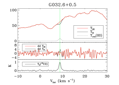
Figure 6.— $Top\ panel$: HINSA spectrum at $\sim 9$ km s^-1 along G032.6+0.5. The observed Hi spectrum ($T\rm_{R}$ ) and derived Hi background spectrum ($T\rm_{H{\textsc{i}}}$) are represented by the black and red solid lines, respectively. The dotted line shows the residual spectrum. During the fitting, the kinetic temperature of CO was fixed at 12 K. The original and fitted optical depths are 0.1 and 0.31. $Middle\ panel$: Second derivatives of Hi and Hi background spectra. $Bottom\ panel$: Corresponding ¹³CO spectrum of HINSA. The green vertical line marks the fitted central velocity of the HINSA cloud from ¹³CO.

HINSA traces the cold component of neutral hydrogen in a molecular cloud which may have a warm Hi halo (Andersson et al., 1991). We were able to determine Hi column density of the Hi halo of molecular clouds with and without HINSA features through the Hi spectra. Due to the omnipresence of Hi in the Galactic plane, we did not apply gaussian decomposition to Hi profiles without HINSA feature. We derived the column density of Hi gas through the integrated Hi intensity. The integrated Hi intensity of recovered background spectrum was used for clouds with HINSA features. With the assumption of low optical depth, the Hi column density $N$(Hi) is given by

$$N({\rm H{\textsc{i}}})=1.82\times 10^{18}\int T_{\rm b}d\upsilon\rm\ cm^{-2},$$ (8)

where the Hi intensity is obtained through integrating the velocity channels determined by OH lines. The effect of adopting different velocity widths of Hi is discussed in Section 5.2.1. $N$(Hi) derived using this method is limited by the optically thin assumption, the intensity contribution from clouds in neighboring velocities, and Hi absorption features corresponding to OH emission lines (e.g., Li & Goldsmith, 2003).

The HINSA column density, $N$(HINSA) derived in 52 clouds ranges from $8.4\times 10^{17}$ cm^-2 to $4.0\times 10^{19}$ cm^-2 with a median value of $8.5\times 10^{18}$ cm^-2, which is 1/36 of the median $N$(Hi) of the Hi halos of these clouds. The median $N$(HINSA) is consistent with that derived in HINSA survey outside the Taurus Molecular Cloud Complex, log${}_{10}(N\rm_{HINSA})$=18.8$\pm$ 0.53 (Krčo & Goldsmith, 2010).

4.4. CO Column Density

Six masks are defined for different detection cases. They are shown in Table 1. When ${}^{12}\rm CO$,${}^{13}\rm CO$ were detected simultaneously (mask 3 and 6 in Table 1), the clouds should be dense molecular gas. In this case, ${}^{12}\rm CO$ is assumed to be optically thick with $\tau_{12}\gg 1$. $T\rm_{ex}^{12}$, the excitation temperature of ${}^{12}\rm CO$, is given by

$$T_{\rm ex}^{12}=5.532\{{\rm ln}[1+\frac{5.532}{T_{\rm b}^{12}+0.819}]\}^{-1},$$ (9)

where $T\rm_{b}^{12}$ is the brightness temperature of ${}^{12}\rm CO$.

The total column density of ¹³CO, $N\rm_{tot}^{{}^{13}CO}$, is given by (Qian et al., 2012)

$$N_{\rm tot}^{\rm{{}^{13}CO}}=3.70\times 10^{14}\int\frac{T_{\rm b}^{13}}{K}\frac{d\upsilon}{\rm km\ s^{-1}}f_{u}f_{\rm\tau_{13}}f_{\rm b}\frac{1}{f_{\rm beam}}\ \rm cm^{-2},$$ (10)

where $T\rm_{b}^{13}$ is the brightness temperature of ${}^{13}\rm CO$. $f_{\tau_{13}}=\int\tau_{13}d\upsilon/\int(1-e^{-\tau_{13}})d\upsilon$ is the correction factor of $\tau_{13}$, the optical depth of $\rm{}^{13}CO(1-0)$. $\tau_{13}$ is given by

$$\tau_{13}=-\rm ln(1-\frac{\textit{T}_{b}^{13}}{\textit{T}_{b}^{12}})\ ,$$ (11)

in which $\tau_{12}\gg 1$ and $T\rm_{ex}^{12}=\textit{T}_{ex}^{13}$ are adopted. These are reasonable when the excitation is dominated by collisions. The Galactic distribution of $\rm{}^{12}C/^{13}C$ ratio derived from synthesized observations of CO,CN, and H₂CO in Milam et al. (2005) was adopted to convert $N(\rm^{13}CO)$ to $N(\rm^{12}CO)$, $\rm{}^{12}C/^{13}C=6.21D_{GC}+18.71$, where $D\rm_{GC}$ is distance to the Galactic center. We adopted the Milky Way rotation curve of Brand & Blitz (1993) to derive $D\rm_{GC}$. Velocity dispersions and non-circular motions (Clemens, 1985) are expected to affect the calculations of $D\rm_{GC}$ with an uncertainty of $<$ 10%, leading to an uncertainty of $\sim$ 1% in $\rm{}^{12}C/^{13}C$.

For clouds with detection of only ${}^{12}\rm CO$ (masks 2 and 5 in Table 1), it is difficult to determine $N(\rm CO)$ without observations of higher lines, e.g., CO(2-1). With the assumption that ${}^{12}\rm CO$ is optically thin, we derive a lower limit. Adoption of a 3$\sigma$ detection of the ${}^{13}\rm CO$ will give an upper limit to the column density. Combining these two facts, we adopted the average value of upper limit and lower limit for $N(^{12}\rm CO)$. Under the optically thin assumption, the total column density of ${}^{12}\rm CO$ can be expressed as

$$N_{\rm tot}^{\rm{}^{12}CO}=3.57\times 10^{14}\int\frac{T_{\rm b}}{K}\frac{d\upsilon}{\rm km\ s^{-1}}f_{u}f_{\tau}f_{b}\frac{1}{f_{\rm beam}}\ \rm cm^{-2},$$ (12)

where $T\rm_{b}$ is the brightness temperature, $f_{u}=Q(T_{\rm ex})/g_{u}{\rm exp}(-h\nu/kT_{\rm ex})$ is the level correction factor, $f_{\tau}=\int\tau_{12}d\upsilon/\int(1-e^{-\tau_{12}})d\upsilon$ is the correction factor of opacity and $f_{\tau}=1$ was adopted under optically thin condition, $f_{\rm b}=1/[1-(e^{h\nu/kT_{\rm ex}}-1)/(e^{h\nu/kT_{\rm bg}}-1)]$ is the correction for the background, $f\rm_{beam}$ is the beam filling factor of the cloud (assumed to be 1.0).

A common excitation temperature of $T\rm_{ex}=12$ K in molecular regions (e.g., Taurus molecular cloud; Goldsmith et al. 2008) was adopted during the calculation. $Q(T_{\rm ex})\approx T_{\rm ex}/2.76$ K is the partition function. $g_{u}$ represents the degeneracy of the upper transition level and equals 3 for CO(1-0) transition. $\tau_{12}$ is the opacity of the ¹²CO(1-0) transition. $\tau_{12}\ll 1$ was assumed, indicating an underestimation of $N(\rm^{12}CO)$ by a factor of $\sim$ 5 when $\tau_{12}=5$. $T\rm_{bg}$ is the background brightness temperature, adopted to be 2.73 K.

A $3\sigma$ upper limit on $\rm{}^{13}CO$ of 0.12 K was adopted in equations 10 and 11 for calculation of the upper limit to $N(\rm^{12}CO)$.

The column density of ¹²CO ranges from $2.7\times 10^{15}$ cm^-2 to $1.2\times 10^{18}$ cm^-2 with a median value of $6.5\times 10^{16}$ cm^-2. The median value of $N(\rm^{12}CO)$ for clouds with both ¹²CO and ¹³CO emission is $9.7\times 10^{16}$ cm^-2, which is $\sim 11$ times that in clouds with ¹²CO emission alone.

5. Results

5.1. Sum Rule of Brightness Temperature

Robinson & McGee (1967) presented a brightness temperature ‘sum rule’, which relates the intensities of the four OH ground-state transitions under the assumptions of small optical depths, a flat background continuum spectrum, and $T\rm_{ex}\gg 0.08$ K. The ‘sum rule’ is,

$$T_{\rm b}(1612)+T_{\rm b}(1720)=T_{\rm b}(1665)/5+T_{\rm b}(1667)/9.$$ (13)

Diffuse OH emission and absorption in the pilot region of SPLASH survey followed this relation, (where “diffuse” OH is defined as signal from the extended molecular ISM, in which maser action is either absent or very weak). Similar to Dawson et al. (2014), we found no deviation from the ‘sum rule’ by more than 3 $\sigma$ for all diffuse OH emission and absorption. An example is shown in Figure 7.

According to Appendix A, the ‘sum rule’ is valid for optically thin condition despite the existence of strong differences between the excitation temperatures of four OH lines. The deviation from the ‘sum rule’ is dominated by the opacity of OH lines. No deviation from the ‘sum rule’ confirms the validity of the optically thin assumption that has been used for calculation in Section 4.2.

Maser amplification, which indicates strong non-LTE behavior and large optical depth, leads to deviation from the ‘sum rule’ as shown in Figure 7. Based on this fact, the ‘sum rule’ can be used as a filter for finding maser candidates.

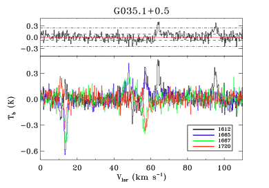
Figure 7.— Top panel: residual spectrum representing $T_{\rm b}(1612)+T_{\rm b}(1720)-T_{\rm b}(1665)/5-T_{\rm b}(1667)/9$. The 1 $\sigma$ and 3 $\sigma$ levels of the spectrum are indicated by in dashed and dash-dotted lines, respectively. Significant deviations are present for the peaks around 64 km s^-1 and 90 km s^-1, which represent an evolved stellar maser associated with the infrared source IRAS 18510+0203. Bottom panel: OH spectra for G035.1+0.5 are displayed as solid lines with different colors.

5.2. Comparison between Different Lines

Hi is the tracer of atomic gas while CO is a tracer of molecular gas. C⁺ emission traces both atomic and molecular gas. All OH clouds have associated Hi emission. Spectra of these lines toward G036.4+0.0 are shown in Figure 3. The statistics of clouds with C⁺ and CO emission corresponding to OH are listed in Table  1. C⁺ and CO are present in 45% and 80% of all the OH clouds, respectively. We present a detailed comparison between column density of Hi, CO line and intensity of C⁺ line with $N$(OH) in the following sections.

Table 1Summary of detections of all 151 OH clouds.

Mask	OH	C+	12CO	13CO	Numbera	HINSAb
1	$\surd$	x	x	x	17	1
2	$\surd$	x	$\surd$	x	17	5
3	$\surd$	x	$\surd$	$\surd$	50	24
4	$\surd$	$\surd$	x	x	10	1
5	$\surd$	$\surd$	$\surd$	x	9	2
6	$\surd$	$\surd$	$\surd$	$\surd$	48	16

5.2.1 Comparison between OH and Hi data

There exist uncertainties in both the OH and Hi data. Thus we adopt the IDL procedure $fitexy.pro$ for fitting, which considers uncertainties in both x and y directions (corresponding to $\rm logN(OH)$ and $\rm logN$(Hi), respectively) during linear least-squares fitting. The value of the fitted slope is larger than that when x error is not considered during fitting (see Table 2 for comparison).

As shown in Table 2, the linear fit for clouds with HINSA in Figure 8 is expressed as, ${\rm log}N$(Hi)=$0.20^{+0.20}_{-0.20}\ {\rm log}N(\rm OH)$+$15.9^{+3.1}_{-3.1}$. The value of the slope is 0.20 with an uncertainty of 0.20, indicating a weak correlation. The linear fit for Hi halo is ${\rm log}N$(Hi)=$1.05^{+0.03}_{-0.03}\ {\rm log}N(\rm OH)+4.57^{+0.43}_{-0.43}$. The value of the slope is 1.0 with an uncertainty of 0.028, indicating a strong correlation. These results show that the correlation between OH and warm Hi is better than that between OH and HINSA. This seems to conflict with the fact that cold Hi rather than warm Hi is mixed with molecular gas (e.g., Goldsmith & Li, 2005). The explanation may be in part the following.

1. Goldsmith & Li (2005) studied local dark clouds not in directions toward the Galactic plane. There was thus little velocity ambiguity for these observations. In the present study of sightlines along the Galactic plane, the OH velocity width was used for calculating $N$(Hi) for Hi halo gas. This may produce a bias toward apparent correlation.

   We note that the velocity width for the Hi halo is always larger than that of molecular tracers, e.g., CO. But no strong correlation between them is found (Andersson et al., 1991). Lee et al. (2012) compared correlation between derived $N$(Hi) with different Hi widths and 2MASS extinction, finding the best correlation between Hi emission and extinction at 20 km s^-1around the CO velocities. The width is much larger than linewidth found for CO, OH, and Hi self-absorption, making such a correlation suspicious. The logic here almost runs in a circle if one tries to study the behavior of Hi associated H₂ by only looking at the velocity range best associated with H₂. The analysis toward clouds in the Galactic plane is more complicated. Firstly, the extinction along a sightline represents sum of all clouds in this sightline. Secondly, the brightness temperature in velocity range of a molecular cloud would be diluted by extended emission of other clouds in this sightline. Thus, we adopted the OH velocity range to calculate Hi column density of to examine the possible Hi halo around our targets.

2. Two correlations with contrary behavior exist between HINSA and OH. Firstly, HINSA content has a positive correlation with increasing molecular cloud size, which can be represented by N(OH). Secondly, Hi is depleted to form H₂, leading decreasing N(HINSA) as the proportion of OH increases. If these two factors are comparable, the absence of correlation between HINSA column density and OH column density is expected.

A feature in Figure 8 is that $N$(Hi) trends to saturate at $1.0\times 10^{21}$ cm^-2 when $N\rm(OH))\gtrsim 4.5\times 10^{15}$ cm^-2. A similar feature is seen in Spider and Ursa Major cirrus clouds, where the asymptotic value of $N$(Hi) is $5\times 10^{20}$ cm^-2 when $N(\rm OH)>0.25\times 10^{14}$ cm^-2 (Barriault et al., 2010). The asymptotic values of $N$(Hi) between this study and Barriault et al. (2010) are consistent but the critical value of $N(\rm OH)$ in this paper is larger by two orders of magnitude. This asymptotic behavior implies that the mass of Hi halo will be same for different clouds when the molecular core is large enough. This behavior also implies that a portion of molecular gas may be not well traced by Hi in the halo.

Table 2 Fitting information in Figure 8 (ID 1 and 2) and Figure 10 (ID 3).

ID	Parameters	Category	Fitted slopea	Fitted intercepta	Fitted slope (SLLS)b
1	N($\rm H{\textsc{i}}$) vs N(OH)	Hi halo	1.05 $\pm$ 0.03	4.57 $\pm$ 0.43	0.58$\pm$ 0.07
2	N($\rm H{\textsc{i}}$) vs N(OH)	HINSA	0.20 $\pm$ 0.20	15.9 $\pm$ 3.1	0.14 $\pm$ 0.18
3	I(C+) vs N(OH)	CO-dark	0.63 $\pm$ 0.46	-9.44 $\pm$ 7.12	0.51 $\pm$ 0.20

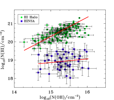
Figure 8.— Hi column density, $N(\rm H{\textsc{i}})$ in HINSA and Hi halo versus OH column density, $N$(OH). Integrated emission spectra were used to derive $N(\rm H{\textsc{i}})$ in Hi halo. The two red solid lines show linear fit for two category of samples.

5.2.2 Comparison between OH and CO data

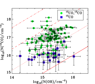
Figure 9.— Comparison of $N(\rm^{12}CO)$ with $N(\rm OH)$ on a log-log scale for 100 clouds. The green filled circles represent 24 OH clouds with ¹²CO emission alone. The blue filled squares represent 76 OH clouds with both ¹²CO and ¹³CO emission. Solid, dotted, dashed, and dash dotted lines represent $N$(CO)/$N$(OH) values of 1, 15, 225, and 3375, respectively. The error bars of $N(^{12}\rm CO)$ for clouds with ${}^{12}\rm CO$ detections represent upper and lower limits. For clouds with detections of both ${}^{12}\rm CO$ and ${}^{13}\rm CO$, statistical uncertainties of the CO spectrum are given. The uncertainty of $N\rm(OH)$ is the same as that described in Figure 8.

The OH column densities are compared with ¹²CO column densities in Figure 9. There is no obvious correlation between $N$(¹²CO) and $N$(OH). A possible reason for this is that OH may reveal larger fraction of molecular gas than CO, e.g., the “CO-dark” gas component, the fraction of which can reach 0.3 even in CO emission clouds (Wolfire et al., 2010).

The ratio between CO and OH column density, $N$(CO)/$N$(OH) varies from 3.7 to $1.6\times 10^{3}$ with a median value of 59 for clouds with both ¹²CO and ¹³CO emission. It varies from 0.81 to 52 with a median value of 7.1 for clouds with only ¹²CO emission. These results confirm that OH will be depleted to form CO, resulting in larger $N$(CO)/$N$(OH) ratios in more massive molecular clouds.

5.2.3 Comparison between OH and C⁺ Emission

The C⁺ 158 $\mu$m fine-structure transition is sensitive to column density, volume density, and kinetic temperature of Hi and H₂, making it difficult to determine C⁺ column density based on present data. We adopted C⁺ intensity rather than C⁺ column density as a parameter for comparison. C⁺ emission can be produced by both photon-dominated regions (PDRs) and the ionized gas in H ii regions. The average ratio of C⁺ emission from H ii and PDRs in IC 342 is 70:30 (Röllig et al., 2016). This fact is included in estimating the uncertainty of C⁺ intensity. We compared the relation between I(C⁺) and N(OH) in CO-dark clouds (mask 4) and molecular clouds (mask 5 and 6).

The clouds were divided into two categories, CO-bright and CO-dark. As seen in Figure 10, no correlation was found between $I(\rm C^{+})$ and $N$(OH) for CO-bright category. But this comparison is limited by the large uncertainty in the C⁺ data and the fact that C⁺ traces both atomic and molecular components. For the CO-dark category, the fitted slope is $0.63\pm 0.46$ (Table 2) with fitted Chi-squre $\chi^{2}=1.84$, indicating a linear correlation. Based on the fact that C⁺ is a good tracer of H₂ in not well-shielded gas (e.g., Pineda et al., 2013), the correlation is consistent with the suggestion that OH is a better trace of H₂ than CO in diffuse clouds, though the sample size is small.

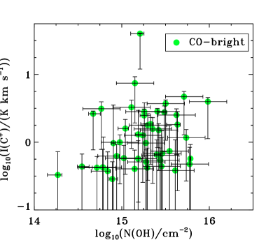
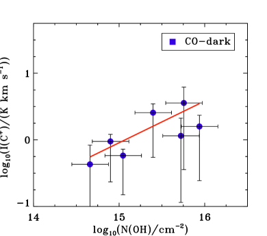
Figure 10.— Comparison of C⁺ intensity with OH column densities on a log-log scale for 54 clouds. Statistical uncertainty of C⁺ spectrum is shown in error bar of C⁺ intensity. The uncertainty in $N\rm(OH)$ is the same as that described in Figure 8. $Left:$ Forty-seven CO-bright clouds with CO emission are indicated by green filled circles. $Right:$ Seven CO-dark clouds without CO emission are indicated by blue circles. The red solid line represents a linear fit to these clouds.

6. Discussion

6.1. OH Column Density

Crutcher (1979) found that OH column density is proportional to the extinction following $N({\rm OH})/A_{\rm V}\approx 8\times 10^{13}$ cm^-2 mag^-1 in $A\rm_{V}$ within the range of 0.4–7 mag, which implies OH/H $\approx 4\times 10^{-8}$. The minimum value of $N$(OH) found in this study is $1.8\times 10^{14}$ cm^-2, which corresponds to an extinction of 2.3 mag. If the $N({\rm OH})/A_{\rm V}$ relation extends to higher extinction, the maximum and median $N$(OH) values would correspond to 138 mag and 24 mag. The value of 24 mag is comparable to the largest extinction in Taurus cloud (Pineda et al., 2010) while the value of 138 mag requires more dense gas. One possible reason is that the value of $N({\rm OH})/A_{\rm V}$ is larger than $8\times 10^{13}$ cm^-2 mag^-1 when $A\rm_{V}>7$ mag. The other reason is that we may have overestimated $N$(OH).

Some satellite lines of OH show ‘flip’ feature inverting from emission to absorption at a velocity. An example is shown in Figure 2. This feature can be interpreted with overlap of infrared transition of OH and implies a transition column density of $N\rm_{OH}/\Delta V\approx 10^{15}$ cm^-2 km^-1 s, where $\rm\Delta V$ is the full width at half-maximum of OH line (e.g., Crutcher, 1977; Brooks & Whiteoak, 2001). These ‘flip’ features were found in three clouds of this survey. The values of N(OH) for ‘flip’ feaure in these clouds can be derived. To compare the results that derived with non-LTE assumption in Section 4.2, we listed calculated $N$(OH) with two different methods in Table 3. The results are consistent within a factor of 2.5, confirming the validity of our calculation of $N$(OH) in Section 4.2.

Table 3 OH column density for three clouds with ‘flip’ of satellite lines.

Sightline	Vlsr	$\Delta\rm V_{1667}$	N(OH)non-LTEa	N(OH)flipb
	km s-1	km s-1	$10^{15}$ cm-2	$10^{15}$ cm-2
G033.8-0.5	11.0	1.3	$0.56_{-0.1}^{+0.04}$	1.3
G033.8+0.0	55.2	2.7	$6.3^{+4.1}_{-2.4}$	2.7
G035.1+1.0	13.2	1.6	$1.3^{+0.1}_{-0.3}$	1.6

6.2. CO-dark Molecular Gas and Atomic/Molecular Transition

A large fraction of molecular gas is expected to exist in the transition region between the fully molecular CO region and the purely atomic Hi region. The molecular gas in this region, which is called the “CO-dark molecular gas” (DMG), cannot be traced by CO, but is associated with ions or molecules that are precursors of CO formation. C⁺ and OH are two of them. One example of a DMG cloud is shown around a velocity of 41.9 km s^-1 in Figure 3. There exist OH and C⁺ emission without corresponding ¹²CO detections with a sensitivity of 0.07 K. Twenty seven DMG clouds, which comprise 18% of all OH clouds, are identified as shown in Table 1. This fraction is smaller than that of $\sim 0.5$ found in pilot OH survey toward Outer Galaxy (Allen et al., 2015). The CO sensitivity of 0.05 K in Allen et al. (2015) is comparable to that in this study. But the OH sensitivity of $\sim 3.0$ mK in Allen et al. (2015) is ten times lower than that in this study. This comparison indicates that the DMG fraction detected depends on OH sensitivity. Higher DMG fraction is expected with higher OH sensitivity.

The DMG can be a significant fraction even in clouds with CO emission (Wolfire et al., 2010) and in observations (e.g., Grenier et al., 2005; Langer et al., 2014; Tang et al., 2016). The fact that the DMG can be traced by OH may explain the absence of correlation between OH and CO in Figure 9.

C⁺ is the main reservoir of carbon in diffuse gas. It converts to CO quickly through C⁺-OH chemical reactions once OH is formed (e.g., van Dishoeck & Black, 1988). Thus C⁺ and OH are expected to have a tight correlation. As shown in Figure 10, a $I(\rm C^{+})$-$N$(OH) correlation may exist for DMG clouds but not for all clouds.

The atomic to molecular transition occurs in the DMG region. Though HINSA other than warm Hi gas is associated with molecular formation, the Hi halo outside the DMG region provides shielding from UV radiation. The asymptotic value of $N$(Hi), $1.0\times 10^{21}$ cm^-2 in Figure 8, corresponding visual extinction $A\rm_{V}$ of 0.5 mag, approaching extinction $A\rm_{V}=0.5-1$ mag (e.g., van Dishoeck & Black, 1988) required to provide effective shielding for CO formation. This extinction of 0.5 mag is much larger than that required for forming abundant H₂, which has a large self-shielding coefficient and can be the dominant form of hydrogen even when $A\rm_{V}>0.02$ mag (Wolfire et al., 2010). Thus a large fraction of DMG will exist before abundant CO formation.

7. Conclusions

We have obtained OH spectra of four 18 cm lines toward 51 GOT C+ sightlines with the Arecibo telescope. Using Gaussian decomposition, we identified 151 OH components. A combined analysis of OH, CO,Hi , and HINSA reveals the following results.

1. OH emission is detected in both main and satellite lines in the inner Galactic plane but is only detected in the main lines in the outer galaxy. A large fraction of detected main lines show absorption features in the inner galaxy but no OH absorption feature was found in the outer galaxy. This is in agreement with more molecular gas and a higher level of continuum background emission being present in the inner galaxy than in the outer galaxy.

2. There is no deviation from the ‘sum rule’ by more than 3$\sigma$ for all of the detected diffuse OH emission, suggesting small opacities of OH lines for clouds in the Galactic plane.

3. The Hi column density $N$(Hi) in the Hi cloud halos has an obvious correlation with the OH column density $N$(OH) following ${\rm log}N$(Hi)=$1.05^{+0.03}_{-0.03}\ {\rm log}N(\rm OH)+4.57^{+0.43}_{-0.43}$. $N$(Hi) reaches an asymptotic value of $1.0\times 10^{21}$ cm^-2 when $N\rm(OH)>4.5\times 10^{15}$ cm^-2.

4. No correlation was found between the cold Hi column density $N$(HINSA) from Hi narrow self-absorption feature and $N$(OH).

5. $N\rm(OH)$/$N\rm(CO)$ ratios are ten times lower in translucent clouds with only ¹²CO detection than in dense clouds with both ¹²CO and ¹³CO detections. This confirms that OH is depleted to form CO. No correlation between $N\rm(OH)$ and $N\rm(CO)$ was found.

6. A weak correlation was found between C⁺ intensity $I\rm(C^{+})$ and $N$(OH) for CO-dark molecular clouds. This is consistent with OH being better tracer of H₂ in diffuse molecular clouds as C⁺ traces H₂ well in not well-shielded gas. No correlation was found for $I\rm(C^{+})$ and $N$(OH) for CO-bright molecular clouds.

Appendix A Derivation of Sum Rule

The column densities of upper and lower levels of each transition, $N\rm_{i}$ and $N\rm_{j}$, are related by

$$\frac{N_{\rm i}}{N_{\rm j}}=\frac{g_{\rm i}}{g_{\rm j}}e^{-h\nu/kT_{\rm ij}}$$ (A1)

where $T\rm_{ij}^{ex}$ is the excitation temperature of OH transition line, $N\rm_{i}$ and $N\rm_{j}$ are partition weight the OH transition, and $g\rm_{i}$ and $g\rm_{j}$ are the statistical weights of i and j levels, respectively. For OH lines, $g=2F+1$, where F is the total angular momentum quantum number. The transition of 1612 MHz gives

$$\frac{N_{3}}{N_{2}}=\frac{g(F=1)}{g(F=2)}e^{-h\nu_{1612}/kT_{1612}}.$$ (A2)

$N_{3}$ and $N_{2}$ are upper and lower level of 1612 MHz line as shown in Figure 11.

Similarly, $\frac{N_{3}}{N_{1}}$,$\frac{N_{4}}{N_{2}}$, and $\frac{N_{4}}{N_{1}}$ are derived from 1665, 1667, and 1720 MHz transitions, respectively. Considering the fact that $\frac{N_{3}}{N_{2}}\times\frac{N_{4}}{N_{1}}$=$\frac{N_{3}}{N_{1}}\times\frac{N_{4}}{N_{2}}$, we have

$$\frac{\nu_{1612}}{T_{1612}}+\frac{\nu_{1720}}{T_{1720}}=\frac{\nu_{1665}}{T_{1665}}+\frac{\nu_{1667}}{T_{1667}}.$$ (A3)

The optical depth $\tau_{\nu}$ at frequency $\nu$ is given by

$$\tau_{\nu}=\frac{c^{2}}{8\pi}\frac{A_{\rm ij}}{\nu^{2}}N_{\rm i}(e^{h\nu_{\rm ij}/kT_{\rm ij}}-1)\phi(\nu).$$ (A4)

With $h\nu_{\rm ij}/kT_{\rm ij}\ll 1$ for OH lines in general, we derive

$$\frac{\nu_{\rm ij}}{T_{\rm ij}}=\frac{8\pi}{c^{2}}\frac{k}{h}\frac{\nu_{\rm ij}^{2}}{A_{\rm ij}N_{\rm i}}\int\tau_{\nu}d\nu.$$ (A5)

When most OH molecules are in the ground state of ${}^{2}\Pi_{3/2}(J=3/2)$, the total OH column density, $N\rm_{OH}$, is sum of molecules in four energy levels, $N\rm_{OH}$=$N_{1}+N_{2}+N_{3}+N_{4}$=$16/3N_{3}$=$16/5N_{4}$. $\int\tau_{\nu}d\nu=\tau_{\nu}^{\rm peak}\Delta V/0.93$, where $\tau_{\nu}^{\rm peak}$ is peak optical depth and $\Delta V$ is full width at half maximum of transition line. Combining equations A3, equation A5, and values of four OH transition coefficients, we derive

$$\tau_{1612}+\tau_{1720}=\tau_{1665}/5+\tau_{1667}/9,$$ (A6)

where $\tau_{1612}$,$\tau_{1720}$,$\tau_{1665}$,and $\tau_{1667}$ are peak optical depth of four OH transitions. The only requirement for Equation A6 is $h\nu_{\rm ij}/kT_{\rm ij}\ll 1$. Thus Equation A6 is valid even for non-LTE conditions.

The brightness of emission line, $T\rm_{b}$, is calculated through $T_{\rm b}=(T_{\rm ex}-T_{\rm bg})(1-e^{-\tau})$, where $T\rm_{bg}$ is background continuum temperature, $\tau$ is optical depth of transition line. When $T_{\rm ex}-T_{\rm bg}$ is the same for the four OH lines, which is valid under LTE conditions, we derive the ‘sum rule’ for brightness temperature under optically thin conditions

$$T_{\rm b}(1612)+T_{\rm b}(1720)=T_{\rm b}(1665)/5+T_{\rm b}(1667)/9.$$ (A7)

To estimate the contribution of non-LTE and optical depth leading to deviation from Equation A7, we plot deviation fraction and maximum optical depth of OH as function of $T\rm_{ex}(1665)$ and $N$(OH) in Figure 12. The deviation from the sum rule (DSR) is significant when $N$(OH) $\geq 2.0\times 10^{15}$ cm^-2. In this parameter space with significant deviation, the optical depth of OH lines $\tau\rm_{max}$(OH) is greater than 0.5. We conclude that the condition of large optical depth results in significant DSR.

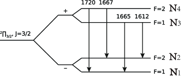
Figure 11.— Energy levels responsible for the OH lines. This figure is reproduced from Dawson et al. (2014).

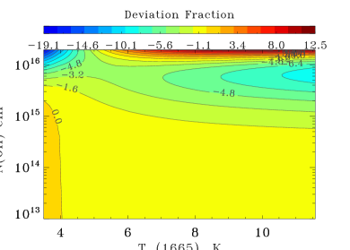
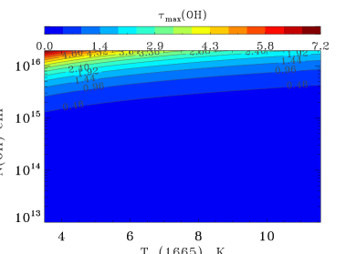
Figure 12.— Top: Contour of deviation fraction of the brightness sum rule, $f$=[$T\rm_{b}(1612)$+$T\rm_{b}(1720)$-$T\rm_{b}(1665)/5$-$T\rm_{b}(1667)/9$]/$\sigma\rm_{spec}$, as a function of $T\rm_{ex}(1665)$ and total OH column density $N\rm_{tot}$(OH). $\sigma\rm_{spec}=42$ mK is the rms of the summed spectra. $T_{\rm ex}(1667)-T_{\rm ex}(1665)=1.0$ K, $T\rm_{ex}(1720)=4.0$ K, and continuum brightness temperature at 1667 MHz of 5.0 K are assumed. $T\rm_{c}$ at 1612 MHz is calculated through $T\rm_{c}(1612)$=3.1+$(T\rm_{c}(1667)-3.1)(1612/1667)^{2.1}$. The continuum brightness at 1720 MHz is calculated using similar method. Bottom: Contour of the maximum optical depth of OH lines.

References

- Allen et al. (2015) Allen, R. J., Hogg, D. E., & Engelke, P. D. 2015, AJ, 149, 123
- Allen et al. (2012) Allen, R. J., Ivette Rodrḿissingguez, M., Black, J. H., & Booth, R. S. 2012, AJ, 143, 97
- Andersson et al. (1991) Andersson, B.-G., Wannier, P. G., & Morris, M. 1991, ApJ, 366, 464
- Barriault et al. (2010) Barriault, L., Joncas, G., Lockman, F. J., & Martin, P. G. 2010, MNRAS, 407, 2645
- Beuermann et al. (1985) Beuermann, K., Kanbach, G., & Berkhuijsen, E. M. 1985, A&A, 153, 17
- Brand & Blitz (1993) Brand, J., & Blitz, L. 1993, A&A, 275, 67
- Brooks & Whiteoak (2001) Brooks, K. J., & Whiteoak, J. B. 2001, MNRAS, 320, 465
- Calabretta et al. (2014) Calabretta, M. R., Staveley-Smith, L., & Barnes, D. G. 2014, PASA, 31, e007
- Clemens (1985) Clemens, D. P. 1985, ApJ, 295, 422
- Cotten et al. (2012) Cotten, D. L., Magnani, L., Wennerstrom, E. A., Douglas, K. A., & Onello, J. S. 2012, AJ, 144, 163
- Crutcher (1979) Crutcher, R. M. 1979, ApJ, 234, 881
- Crutcher (1977) Crutcher, R. M. 1977, ApJ, 216, 308
- Dame et al. (2001) Dame, T. M., Hartmann, D., & Thaddeus, P. 2001, ApJ, 547, 792
- Dawson et al. (2014) Dawson, J. R., Walsh, A. J., Jones, P. A., et al. 2014, MNRAS, 439, 1596
- Dickey et al. (1981) Dickey, J. M., Crovisier, J., & Kazes, I. 1981, A&A, 98, 271
- Giardino et al. (2002) Giardino, G., Banday, A. J., Górski, K. M., et al. 2002, A&A, 387, 82
- Gibson et al. (2000) Gibson, S. J., Taylor, A. R., Higgs, L. A., & Dewdney, P. E. 2000, ApJ, 540, 851
- Goldsmith & Li (2005) Goldsmith, P. F., & Li, D. 2005, ApJ, 622, 938
- Goldsmith et al. (2008) Goldsmith, P. F., Heyer, M., Narayanan, G., et al. 2008, ApJ, 680, 428-445
- Grenier et al. (2005) Grenier, I. A., Casandjian, J.-M., & Terrier, R. 2005, Science, 307, 1292
- Grossmann et al. (1990) Grossmann, V., Heithausen, A., Meyerdierks, H., & Mebold, U. 1990, A&A, 240, 400
- Guibert et al. (1978) Guibert, J., Rieu, N. Q., & Elitzur, M. 1978, A&A, 66, 395
- Haslam et al. (1982) Haslam, C. G. T., Salter, C. J., Stoffel, H., & Wilson, W. E. 1982, A&AS, 47, 1
- Heiles (1969) Heiles, C. 1969, ApJ, 157, 123
- Heiles (1968) Heiles, C. E. 1968, ApJ, 151, 919
- Jackson et al. (2002) Jackson, J. M., Bania, T. M., Simon, R., et al. 2002, ApJ, 566, L81
- Krčo et al. (2008) Krčo, M., Goldsmith, P. F., Brown, R. L., & Li, D. 2008, ApJ, 689, 276-289
- Krčo & Goldsmith (2010) Krčo, M., & Goldsmith, P. F. 2010, ApJ, 724, 1402
- Langer et al. (2010) Langer, W. D., Velusamy, T., Pineda, J. L., et al. 2010, A&A, 521, L17
- Langer et al. (2014) Langer, W. D., Velusamy, T., Pineda, J. L., Willacy, K., & Goldsmith, P. F. 2014, A&A, 561, A122
- Lee et al. (2012) Lee, M.-Y., Stanimirović, S., Douglas, K. A., et al. 2012, ApJ, 748, 75
- Li & Goldsmith (2003) Li, D., & Goldsmith, P. F. 2003, ApJ, 585, 823
- Li et al. (2015) Li, D., Xu, D., Heiles, C., Pan, Z., & Tang, N. 2015, Publication of Korean Astronomical Society, 30, 75
- Liszt & Lucas (1996) Liszt, H., & Lucas, R. 1996, A&A, 314, 917
- Liszt & Pety (2012) Liszt, H. S., & Pety, J. 2012, A&A, 541, A58
- Mather et al. (1994) Mather, J. C., Cheng, E. S., Cottingham, D. A., et al. 1994, ApJ, 420, 439
- Milam et al. (2005) Milam, S. N., Savage, C., Brewster, M. A., Ziurys, L. M., & Wyckoff, S. 2005, ApJ, 634, 1126
- Myers (1975) Myers, P. C. 1975, ApJ, 198, 331
- Nakanishi & Sofue (2003) Nakanishi, H., & Sofue, Y. 2003, PASJ, 55, 191
- Nguyen-Q-Rieu et al. (1976) Nguyen-Q-Rieu, Winnberg, A., Guibert, J., et al. 1976, A&A, 46, 413
- Peek et al. (2011) Peek, J. E. G., Heiles, C., Douglas, K. A., et al. 2011, ApJS, 194, 20
- Penzias (1964) Penzias, A. A. 1964, AJ, 69, 146
- Pineda et al. (2010) Pineda, J. L., Goldsmith, P. F., Chapman, N., et al. 2010, ApJ, 721, 686
- Pineda et al. (2013) Pineda, J. L., Langer, W. D., Velusamy, T., & Goldsmith, P. F. 2013, A&A, 554, A103
- Planck Collaboration et al. (2011) Planck Collaboration, Ade, P. A. R., Aghanim, N., et al. 2011, A&A, 536, A19
- Qian et al. (2012) Qian, L., Li, D., & Goldsmith, P. F. 2012, ApJ, 760, 147
- Röllig et al. (2016) Röllig, M., Simon, R., Güsten, R., et al. 2016, A&A, 591, A33
- Reich & Reich (1986) Reich, P., & Reich, W. 1986, A&AS, 63, 205
- Robinson & McGee (1967) Robinson, B. J., & McGee, R. X. 1967, ARA&A, 5, 183
- Roman-Duval et al. (2009) Roman-Duval, J., Jackson, J. M., Heyer, M., et al. 2009, ApJ, 699, 1153
- Tang et al. (2016) Tang, N., Li, D., Heiles, C., et al. 2016, A&A, 593, A42
- Turner (1973) Turner, B. E. 1973, ApJ, 186, 357
- Turner & Heiles (1971) Turner, B. E., & Heiles, C. 1971, ApJ, 170, 453
- Turner (1979) Turner, B. E. 1979, A&AS, 37, 1
- van Dishoeck & Black (1988) van Dishoeck, E. F., & Black, J. H. 1988, ApJ, 334, 771
- Wannier et al. (1993) Wannier, P. G., Andersson, B.-G., Federman, S. R., et al. 1993, ApJ, 407, 163
- Weinreb et al. (1963) Weinreb, S., Barrett, A. H., Meeks, M. L., & Henry, J. C. 1963, Nature, 200, 829
- Wolfire et al. (2010) Wolfire, M. G., Hollenbach, D., & McKee, C. F. 2010, ApJ, 716, 1191