Numerical Simulation of Bloch Equations for
Dynamic Magnetic Resonance Imaging

Abstract

Magnetic Resonance Imaging (MRI) is a widely applied non-invasive imaging modality based on non-ionizing radiation which gives excellent images and soft tissue contrast of living tissues. We consider the modified Bloch problem as a model of MRI for flowing spins in an incompressible flow field. After establishing the well-posedness of the corresponding evolution problem, we analyze its spatial semi-discretization using discontinuous Galerkin methods. The high frequency time evolution requires a proper explicit and adaptive temporal discretization. The applicability of the approach is shown for basic examples.

1 Bloch Model for Magnetic Resonance Imaging

Magnetic Resonance Imaging (MRI) is a non-invasive imaging modality based on non-ionizing radiation [1]. It gives excellent images and soft tissue contrast of living tissues. During the experiment, the object to be studied is placed in a static magnetic field of high strength $B_{0}$. This induces a macroscopic nuclear magnetization $\mathbf{M}_{0}$ in the direction of magnetic field, known as the equilibrium magnetization. The direction of equilibrium magnetization is called the longitudinal direction, generally denoted by the $z$-axis as in Fig. 1.

In order to get a response from the object, the equilibrium magnetization is perturbed by applying a short radio-frequency (RF) pulse $\mathbf{B}_{1}$ in the transverse plane (denoted by the $xy$-plane in Fig. 1) with the excitation carrier frequency of the RF pulse equal to the Larmor frequency of protons. As a result, the equilibrium magnetization is flipped from its initial position towards the transverse plane. The perturbation of equilibrium magnetization depends on the duration and magnitude of the RF field. After the RF pulse is switched off, the magnetization precesses towards its equilibrium position. This process is known as relaxation. The relaxation of magnetization is governed by two time constants - spin-lattice time relaxation $T_{1}$, spin-spin time relaxation $T_{2}$, as illustrated in Fig. 1.

Figure 1: Schematic of a pulsed MR experiment on net Magnetization $\mathbf{M}$. Left: $\mathbf{M}$ align along the static magnetic field $B_{0}$. Second from left: RF excitation perturbs the magnetization from the longitudinal direction. Middle: Precession of magnetization as a result of, Second from right: $T_{2}$ decay. Right: $T_{1}$ recovery.

On top of that magnetic field gradients need to be applied to obtain cross-sectional images. The location and thickness of the slice is determined by applying a slice-selection gradient $G_{z}$. After that, the object is spatially encoded via the application of additional magnetic field gradients $G_{x},G_{y}$ in the transversal directions. The magnitude and time of application of magnetic gradients $\mathbf{G}$ depend on the experimental requirements, see Sec. 5 for the description of a typical pulse sequence.

The Bloch equation [2] for MRI combines all of the above components: static magnetic field $\mathbf{B_{0}}$, time-dependent magnetic gradients $\mathbf{G}(t)$ and the RF pulse $\mathbf{B}_{1}(t)=(B_{x}(t),B_{y}(t),0)^{T}$ and is given by

$$\mathinner{\dfrac{\operatorname{d\!}{}\mathbf{M}}{\operatorname{d\!}{t}}} =\gamma\mathbf{M}\times\mathbf{B}+\frac{M_{0}-M_{z}}{T_{1}}\hat{e}_{z}-\frac{M_{x}}{T_{2}}\hat{e}_{x}-\frac{M_{y}}{T_{2}}\hat{e}_{y},$$ (1.1)

$$\mathbf{B}(t,\mathbf{r}) =(B_{x}(t),B_{y}(t),B_{z}(t,\mathbf{r}))^{T},\quad B_{z}(t,\mathbf{r})\mathrel{\mathop{\mathchar 58\relax}}=B_{0}+\mathbf{G}(t)\cdot\mathbf{r}.$$

Emitted energy due to the precession of the magnetizations is converted into an electric signal in the receiver coil of an MRI system which is manipulated further for image reconstruction. The received signal can be expressed as

$$s_{r}(t)\varpropto\int_{\Omega}M_{xy}(\mathbf{r},t){\mathrm{e}}^{-i\gamma B_{0}t}{\mathrm{e}}^{-i\gamma\int_{0}^{t}(xG_{x}+yG_{y})d\tau}d\mathbf{r}$$ (1.2)

where $M_{xy}=M_{x}+iM_{y}$. The received signals are typically demodulated in frequency by $\gamma B_{0}$ using phase-sensitive detection before being used for image reconstruction. The resultant signal expression after demodulation is $s_{d}(t)=s_{r}(t){\mathrm{e}}^{i\gamma B_{0}t}$ [1].

The demodulated signal corresponds to the solution of the Bloch equation in a frame rotating clockwise about $z$-axis with an angular frequency $\gamma B_{0}$, i.e, the Larmor frequency of the isocenter of the object. The Bloch equation in the rotating frame conceptually simplifies the RF excitation effect in MRI and eliminates the static $\mathbf{B}_{0}$ field from the expression of the external magnetic field and is given by

$$\mathinner{\dfrac{\operatorname{d\!}{}\mathbf{M}^{\prime}}{\operatorname{d\!}{t}}} =\gamma\mathbf{M}^{\prime}\times\mathbf{B}_{\text{eff}}+\frac{(M_{0}-M_{z})\hat{e}_{z}}{T_{1}}-\frac{M_{x^{\prime}}\hat{e}_{x^{\prime}}+M_{y^{\prime}}\hat{e}_{y^{\prime}}}{T_{2}}$$ (1.3a)

$$=\begin{bmatrix}-\frac{1}{T_{2}}&\gamma B_{z^{\prime}}&-\gamma B_{y^{\prime}}\\ -\gamma B_{z^{\prime}}&-\frac{1}{T_{2}}&\gamma B_{x^{\prime}}\\ \gamma B_{y^{\prime}}&-\gamma B_{x^{\prime}}&-\frac{1}{T_{1}}\end{bmatrix}\begin{pmatrix}M_{x^{\prime}}\\ M_{y^{\prime}}\\ M_{z}\end{pmatrix}+\begin{pmatrix}0\\ 0\\ \frac{M_{0}}{T_{1}}\end{pmatrix},$$ (1.3b)

where $\mathbf{M}^{\prime}(t,\mathbf{r})=(M_{x^{\prime}},M_{y^{\prime}},M_{z})^{T}(t,\mathbf{r})$ represents the magnetization in the rotating frame and the effective magnetic field is given by $\mathbf{B}_{\textnormal{eff}}(t,\mathbf{r})=(B_{x^{\prime}},B_{y^{\prime}},B_{z^{\prime}})^{T}(t,\mathbf{r})$; $B_{z^{\prime}}(t,\mathbf{r})\mathrel{\mathop{\mathchar 58\relax}}=G(t)\cdot\mathbf{r}$.

In order to study the effect of fluid flow in an MRI experiment, the transport of magnetizations due to flow field $\mathbf{u}(t,\mathbf{r})$ must be taken into account and is modeled by the modified Bloch equation [3]:

$$\mathinner{\dfrac{\partial{}\mathbf{M}}{\partial{t}}}+(\mathbf{u}\cdot\bm{\nabla})\mathbf{M} =\gamma\mathbf{M}\times\mathbf{B}+\frac{(M_{0}-M_{z})\hat{e}_{z}}{T_{1}}-\frac{M_{x}\hat{e}_{x}+M_{y}\hat{e}_{y}}{T_{2}}.$$ (1.4)

There will be no diffusion term as effect of diffusion is negligible, but see Sec. 2.

Due to signal demodulation, the signal acquired from the flowing object in an MRI experiment is equivalent to an equation where magnetizations and the magnetic field ($\mathbf{B}_{\text{eff}}$) are written in the rotating frame with velocity $\mathbf{u}(t,\mathbf{r})$ kept in laboratory frame [4]:

$$\mathinner{\dfrac{\partial{}\mathbf{M}^{\prime}}{\partial{t}}}+(\mathbf{u}\cdot\bm{\nabla})\mathbf{M}^{\prime}=\gamma\mathbf{M}^{\prime}\times\mathbf{B_{\text{eff}}}+\frac{(M_{0}-M_{z})\hat{e}_{z}}{T_{1}}-\frac{M_{x^{\prime}}\hat{e}_{x^{\prime}}+M_{y^{\prime}}\hat{e}_{y\prime}}{T_{2}}.$$ (1.5)

For notational simplicity the ^′ will be omitted in later sections. Hereafter, magnetization $\mathbf{M}$ will always be in the rotating frame and the velocity in the laboratory frame.

In the past, Bloch equation based MRI simulators were developed for variety of research directions e.g. optimizing MR sequences, artifact detection, testing image reconstruction techniques, design of specialized RF pulses and educational purposes. Also, multiple utilities of numerical simulations have been combined to produce a few general purpose MRI simulators e.g., [5, 6, 7, 8, 9]. Accurate simulation of this initial-value problem is still challenging for the following reasons: very tiny time steps, sufficiently fine spatial resolution, and non-smooth data (e.g. gradient field $\mathbf{G}$). To overcome this difficulty, the execution speeds were improved using parallelization with message passing interface (MPI), e.g. [8, 6], or GPU e.g. [9]. There are two prevailing techniques for the development of the simulator (i) a semi-analytical technique based on operator splitting as used, e.g., in [8, 9] (ii) coupled approach with fast ODE-solvers [6].

Similarly, there are many numerical studies on the influence of flow on MRI e.g., [10, 11, 4, 12]. Modified Bloch model was solved using multiple numerical strategies previously e.g., Jou et al. [11], Lorthois et al. [4] first solved the flow field in a computational mesh using finite volume method (FVM) softwares and then studied the effect of flow on magnetization using finite difference method (FDM). Jurczuk et al. [12] solved 1.5 by splitting the transport and the MR terms. In their work, the magnetization transport was calculated using lattice-Boltzmann method (LBM) and the reaction part was calculated using operator splitting techniques.

However, the previous studies lack a proper analysis of the Bloch model for flowing objects. Sec. 2 is devoted to prove the well-posedness of the modified Bloch model. The spatial semi-discretization with DG-methods is presented in Sec. 3 which, to the best of our knowledge, is also an addition to the literature related to Bloch model. This section was followed by consideration of the temporal discretization in Sec. 4. Verifications for simple problems for static and flowing objects are presented in Sec. 5.

2 Well-posedeness of the Bloch Model

Let $\Omega\subset\mathbb{R}^{3}$ be the flow domain with piecewise smooth Lipschitz boundary $\Gamma$ and outer normal $\mathbf{n}$. The incompressible flow field $\mathbf{u}(t,\mathbf{r})$ introduces the splitting $\Gamma=\Gamma_{-}\bigcup\Gamma_{+}\bigcup\Gamma_{0}$ where $\Gamma_{-}=\{\mathbf{r}\in\Gamma|\mathbf{u}\cdot\mathbf{n}<0\},\;\Gamma_{+}=\{\mathbf{r}\in\Gamma|\mathbf{u}\cdot\mathbf{n}>0\}\;\textnormal{and}\;\Gamma_{0}=\{\mathbf{r}\in\Gamma|\mathbf{u}\cdot\mathbf{n}=0\}$ represent the inflow boundary, outflow boundary and solid wall, respectively. We assume that inflow and outflow are separated, i.e. $\mbox{dist}(\Gamma_{-},\Gamma_{+})\mathrel{\mathop{\mathchar 58\relax}}=\min_{(P,Q)\in\Gamma_{-}\times\Gamma_{+}}|P-Q|>0$.

Problem 1.5 can be rewritten using $\mathbf{B}_{\textnormal{eff}}=\mathbf{B}=\begin{pmatrix}B_{x},B_{y},B_{z}\end{pmatrix}^{T}$, the relaxation time diagonal matrix $D=\operatorname{diag}(\frac{1}{T_{2}},\frac{1}{T_{2}},\frac{1}{T_{1}})$ and the constant source term $\mathbf{f}=\begin{pmatrix}0,0,\frac{M_{0}}{T_{1}}\end{pmatrix}^{T}$ along with appropriate boundary and initial conditions as

$$\mathinner{\dfrac{\partial{}\mathbf{M}}{\partial{t}}}+(\mathbf{u}\cdot\bm{\nabla})\mathbf{M}+\gamma\mathbf{B}\times\mathbf{M}+D\mathbf{M} =\mathbf{f},\qquad(t,\mathbf{r})\in[0,T]\times\Omega,$$ (2.1a)

$$\mathbf{M} =\mathbf{M}_{\Gamma},\quad(t,\mathbf{r})\in[0,T]\times\Gamma_{-},$$ (2.1b)

$$\mathbf{M} =\mathbf{M}^{0},\quad(t,\mathbf{r})\in\{0\}\times\Omega.$$ (2.1c)

Consider the space ${\mathbf{H}}\mathrel{\mathop{\mathchar 58\relax}}=[L^{2}(\Omega)]^{3}$ with inner product $(\mathbf{u},\mathbf{v})_{\mathbf{H}}\mathrel{\mathop{\mathchar 58\relax}}=\int_{\Omega}\mathbf{u}\cdot\mathbf{v}\leavevmode\nobreak\ \operatorname{d\!}{\mathbf{r}}$ and norm $\mathinner{\!\left\lVert\mathbf{v}\right\rVert}_{\mathbf{H}}\mathrel{\mathop{\mathchar 58\relax}}=\sqrt{(\mathbf{v},\mathbf{v})}$. Moreover, define

$$\mathbf{X}=\{\mathbf{N}\in\mathbf{H}\mathrel{\mathop{\mathchar 58\relax}}\leavevmode\nobreak\ (\mathbf{u}\cdot\bm{\nabla})\mathbf{N}\in{\mathbf{H}}\}$$ (2.2)

with graph norm

$$\|\mathbf{N}\|_{\mathbf{X}}\mathrel{\mathop{\mathchar 58\relax}}=\left(\|(\mathbf{u}\cdot\nabla)\mathbf{N}\|^{2}_{\mathbf{H}}+\|\mathbf{N}\|^{2}_{\mathbf{H}}\right)^{\frac{1}{2}}.$$ (2.3)

Multiplying 2.1a by an arbitrary test function $\mathbf{N}\in\mathbf{X}$, integrating over $\Omega$ and imposing (2.1b) weakly, we obtain

$$(\partial_{t}\mathbf{M},\mathbf{N})_{\mathbf{H}}+((\mathbf{u}\cdot\bm{\nabla})\mathbf{M},\mathbf{N})_{\mathbf{H}}+\gamma(\mathbf{B}\times\mathbf{M},\mathbf{N})_{\mathbf{H}}$$ (2.4)

$$\quad+(D\mathbf{M},\mathbf{N})_{\mathbf{H}}+\int_{\Gamma}(\mathbf{u}\cdot\mathbf{n})^{\ominus}\mathbf{M}\cdot\mathbf{N}\;\operatorname{d\!}{s}=(\mathbf{f},\mathbf{N})_{\mathbf{H}}+\int_{\Gamma}(\mathbf{u}\cdot\mathbf{n})^{\ominus}\mathbf{M}_{\Gamma}\cdot\mathbf{N}\;\operatorname{d\!}{s},$$

where $w^{\ominus}(\mathbf{r})\mathrel{\mathop{\mathchar 58\relax}}=\frac{1}{2}(\mathinner{\!\left\lvert w(\mathbf{r})\right\rvert}-w(\mathbf{r}))$ and $\mathbf{M}\times\mathbf{B}=-\mathbf{B}\times\mathbf{M}$. Define bilinear and linear forms

$$a(t;\mathbf{M},\mathbf{N}) \mathrel{\mathop{\mathchar 58\relax}}=((\mathbf{u}\cdot\bm{\nabla})\mathbf{M},\mathbf{N})_{\mathbf{H}}+\gamma((\mathbf{B}\times\mathbf{M}),\mathbf{N})_{\mathbf{H}}$$

$$+(D\mathbf{M},\mathbf{N})_{\mathbf{H}}+\int_{\Gamma}(\mathbf{u}\cdot\mathbf{n})^{\ominus}\mathbf{M}\cdot\mathbf{N}\operatorname{d\!}{s},$$ (2.5a)

$$l(\mathbf{N}) \mathrel{\mathop{\mathchar 58\relax}}=(\mathbf{f},\mathbf{N})_{\mathbf{H}}+\int_{\Gamma}(\mathbf{u}\cdot\mathbf{n})^{\ominus}\mathbf{M}_{\Gamma}\cdot\mathbf{N}\operatorname{d\!}{s},$$ (2.5b)

Then we obtain the variational form of the Bloch problem: Find $\mathbf{M}\mathrel{\mathop{\mathchar 58\relax}}(0,T]\to X$ s.t.

$$(\partial_{t}\mathbf{M},\mathbf{N})_{\mathbf{H}}+a(t;\mathbf{M},\mathbf{N}) =l(\mathbf{N}),\quad\forall\;\mathbf{N}\in\mathbf{X},$$ (2.6)

$$\mathinner{\mathbf{M}\rvert}_{t=0} =\mathbf{M}^{0}.$$ (2.7)

This is a Friedrichs system, see [13], Sec. 7. Unfortunately, the theory in [13, 14] is not applicable since some coefficients are time-dependent. For $0<\epsilon\ll 1$, we set $\mathbf{X}_{\epsilon}\mathrel{\mathop{\mathchar 58\relax}}=[W^{1,2}(\Omega)]^{3}$ and consider an elliptic regularization of (2.6): Find $\mathbf{M}_{\epsilon}\mathrel{\mathop{\mathchar 58\relax}}(0,T]\to X_{\epsilon}$ s.t.

$$(\partial_{t}\mathbf{M}_{\epsilon},\mathbf{N})_{\mathbf{H}}+a_{\epsilon}(t;\mathbf{M}_{\epsilon},\mathbf{N}) =l(\mathbf{N}),\quad\forall\;\mathbf{N}\in\mathbf{X_{\epsilon}},$$ (2.8)

$$\mathinner{\mathbf{M}_{\epsilon}\rvert}_{t=0} =\mathbf{M}^{0}.$$ (2.9)

with

$$a_{\epsilon}(t;\mathbf{M},\mathbf{N}) \mathrel{\mathop{\mathchar 58\relax}}=a(t;\mathbf{M},\mathbf{N})+\epsilon(\nabla{\mathbf{M}},\nabla{\mathbf{N}})_{\mathbf{H}}.$$ (2.10)

Please note that the variational formulation of the regularized Bloch problem incorporates do-nothing boundary conditions $\epsilon\nabla\mathbf{M}_{\epsilon}\cdot\mathbf{n}=\mathbf{0}$ on $\Gamma_{0}\cup\Gamma_{+}$.

The spaces $\mathbf{X_{\epsilon}}\subseteq\mathbf{H}$ and the dual space $\mathbf{X_{\epsilon}}^{*}$ form an evolution triple $(\mathbf{X_{\epsilon}},\mathbf{H},\mathbf{X_{\epsilon}}^{*})$. For $p\geq 1$ and Banach space $\mathbf{Y}$ we denote by $L^{p}(0,T;\mathbf{Y})$ the Bochner space of vector-valued functions $\mathbf{v}\mathrel{\mathop{\mathchar 58\relax}}(0,T)\to\mathbf{Y}$. We look for a solution $\mathbf{M}_{\epsilon}\in L^{\infty}(0,T;\mathbf{H})\cap L^{2}(0,T;\mathbf{X_{\epsilon}})$ of problem (2.8)-(2.9).

Theorem 2.1 (Well-posedness).

For all $\epsilon>0$, for given $\mathbf{u}\in[L^{\infty}(0,T;W^{1,\infty}(\Omega)]^{3}$ with $\mbox{div}\leavevmode\nobreak\ {\mathbf{u}}=0$ and $\mathbf{B}\in[L^{\infty}(0,T;\mathbf{H})]^{3}$, there exists a unique solution $\mathbf{M}_{\epsilon}\in L^{\infty}(0,T;\mathbf{H})\cap L^{2}(0,T;\mathbf{X_{\epsilon}})$ to Equations 2.8–2.9. For $t\in(0,T]$ and with $\sigma\mathrel{\mathop{\mathchar 58\relax}}=\frac{1}{T_{1}}$, the following a-priori estimate is valid

$$\frac{1}{2}\mathinner{\!\left\lVert\mathbf{M}_{\epsilon}(t)\right\rVert}_{\mathbf{H}}^{2}+\int_{0}^{t}{\mathrm{e}}^{\sigma(\tau-t)}\left[\epsilon\mathinner{\!\left\lVert\nabla\mathbf{M}_{\epsilon}(\tau)\right\rVert}^{2}_{\mathbf{H}}+\frac{1}{2}\int_{\Gamma}|(\mathbf{u}\cdot\mathbf{n})|(\mathbf{M}_{\epsilon}\cdot\mathbf{M}_{\epsilon})(s,\tau)\operatorname{d\!}s\right]\operatorname{d\!}{\tau}$$

$$\leq\frac{1}{2}\mathinner{\!\left\lVert\mathbf{M}_{\epsilon}(0)\right\rVert}_{\mathbf{H}}^{2}{\mathrm{e}}^{-\sigma t}+\frac{1}{2\sigma}\int_{0}^{t}\mathinner{\!\left\lVert\mathbf{f}(\tau)\right\rVert}_{\mathbf{H}}^{2}{\mathrm{e}}^{\sigma(\tau-t)}\;\operatorname{d\!}{\tau}.$$ (2.11)

Proof.

In order to prove well-posedness, we apply the main existence theorem for evolution problems by J.L. Lions, see Theorem 6.6 in [13]. To this end, we define the norm

$$\mathinner{\!\left\lVert\mathbf{M}\right\rVert}_{\mathbf{X}_{\epsilon}}=\left[\epsilon\mathinner{\!\left\lVert\nabla{\mathbf{M}}\right\rVert}^{2}_{L^{2}(\Omega)}+\mathinner{\!\left\lVert\mathbf{M}\right\rVert}^{2}_{\mathbf{X}}\right]^{\frac{1}{2}}.$$ (2.12)

For the application of the theorem, the following conditions must be satisfied:

1. The time-dependent bilinear form $t\mapsto a_{\epsilon}(t;\mathbf{M},\mathbf{N})$ is measurable for all $\mathbf{M},\mathbf{N}\in\mathbf{X}_{\epsilon}$ since the fields $\mathbf{u}$ and $\mathbf{B}$ are sufficiently smooth.

2. Application of the Cauchy-Schwarz and generalized Hölder inequalities show that the bilinear form $a_{\epsilon}(t;\cdot,\cdot)$ is bounded for $t\in[0,T]$ and for all $\mathbf{M},\mathbf{N}\in\mathbf{X}_{\epsilon}$:

   $$\mathinner{\!\left\lvert a_{\epsilon}(t;\mathbf{M},\mathbf{N})\right\rvert}\leq \epsilon\mathinner{\!\left\lVert\nabla{\mathbf{M}}\right\rVert}_{\mathbf{H}}\mathinner{\!\left\lVert\nabla{\mathbf{N}}\right\rVert}_{\mathbf{H}}+\mathinner{\!\left\lvert(\mathbf{u}\cdot\nabla\mathbf{M},\mathbf{N})_{\mathbf{H}}\right\rvert}+\gamma\mathinner{\!\left\lvert(B\times\mathbf{M},\mathbf{N})_{\mathbf{H}}\right\rvert}$$

   $$+\mathinner{\!\left\lvert(D\mathbf{M},\mathbf{N})_{\mathbf{H}}\right\rvert}+\mathinner{\!\left\lvert\int_{\Gamma}(\mathbf{u}\cdot\mathbf{n})^{\ominus}\mathbf{M}\cdot\mathbf{N}\;\operatorname{d\!}{s}\right\rvert}$$

   $$\leq \epsilon\mathinner{\!\left\lVert\nabla{\mathbf{M}}\right\rVert}_{\mathbf{H}}\mathinner{\!\left\lVert\nabla{\mathbf{N}}\right\rVert}_{\mathbf{H}}+\mathinner{\!\left\lVert\mathbf{u}\cdot\nabla\mathbf{M}\right\rVert}_{\mathbf{H}}\mathinner{\!\left\lVert\mathbf{N}\right\rVert}_{\mathbf{H}}+\gamma\mathinner{\!\left\lVert\mathbf{B}\right\rVert}_{L^{\infty}}\mathinner{\!\left\lVert\mathbf{M}\right\rVert}_{\mathbf{H}}\mathinner{\!\left\lVert\mathbf{N}\right\rVert}_{\mathbf{H}}$$

   $$+\mathinner{\!\left\lVert D\right\rVert}_{L^{\infty}}\mathinner{\!\left\lVert\mathbf{M}\right\rVert}_{\mathbf{H}}\mathinner{\!\left\lVert\mathbf{N}\right\rVert}_{\mathbf{H}}+k_{s}\mathinner{\!\left\lVert\mathbf{M}\right\rVert}_{\mathbf{X}}\mathinner{\!\left\lVert\mathbf{N}\right\rVert}_{\mathbf{X}}$$

   with $\mathinner{\!\left\lVert\mathbf{B}\right\rVert}_{\infty}\mathrel{\mathop{\mathchar 58\relax}}=\mathinner{\!\left\lVert\mathbf{B}\right\rVert}_{L^{\infty}(0,T;[L^{\infty}(\Omega)]^{3})}$, $\mathinner{\!\left\lVert D\right\rVert}_{L^{\infty}}\mathrel{\mathop{\mathchar 58\relax}}=\max\{\frac{1}{T_{1}},\frac{1}{T_{2}}\}=\frac{1}{T_{2}}$ as $T_{1}\geq T_{2}$ and where we used the trace inequality (see [14], Lemma $2.5$)

   $$\mathinner{\!\left\lvert\int_{\Gamma}(\mathbf{u}\cdot\mathbf{n})^{\ominus}\mathbf{M}\cdot\mathbf{N}\;\operatorname{d\!}{s}\right\rvert}\leq k_{s}\mathinner{\!\left\lVert\mathbf{u}\cdot\nabla\mathbf{M}\right\rVert}_{\mathbf{H}}\mathinner{\!\left\lVert\mathbf{u}\cdot\nabla\mathbf{N}\right\rVert}_{\mathbf{H}}\leq k_{s}\mathinner{\!\left\lVert\mathbf{M}\right\rVert}_{\mathbf{X}}\mathinner{\!\left\lVert\mathbf{N}\right\rVert}_{\mathbf{X}}.$$

   Now the norm definitions (2.3) and (2.12) imply boundedness:

   $$\mathinner{\!\left\lvert a_{\epsilon}(t;\mathbf{M},\mathbf{N})\right\rvert}\leq (2+\gamma\mathinner{\!\left\lVert\mathbf{B}\right\rVert}_{L^{\infty}}+\mathinner{\!\left\lVert D\right\rVert}_{L^{\infty}}+k_{s})\mathinner{\!\left\lVert\mathbf{M}\right\rVert}_{\mathbf{X_{\epsilon}}}\mathinner{\!\left\lVert\mathbf{N}\right\rVert}_{\mathbf{X_{\epsilon}}}.$$

3. Finally, bilinear form $a_{\epsilon}$ fulfills a coercivity condition. Integration by parts yields

   $$a_{\epsilon}(t;\mathbf{N},\mathbf{N}) =\epsilon\mathinner{\!\left\lVert\nabla\mathbf{N}\right\rVert}^{2}_{\mathbf{H}}+\mathinner{\!\left\lVert D^{\nicefrac{{1}}{{2}}}\mathbf{N}\right\rVert}^{2}_{\mathbf{H}}+\frac{1}{2}\int_{\Gamma}(\mathbf{u}\cdot\mathbf{n})\mathbf{N}\cdot\mathbf{N}\;\operatorname{d\!}{s}+\int_{\Gamma}(\mathbf{u}\cdot\mathbf{n})^{\ominus}\mathbf{N}\cdot\mathbf{N}\;\operatorname{d\!}{s}$$

   $$=\epsilon\mathinner{\!\left\lVert\nabla\mathbf{N}\right\rVert}^{2}_{\mathbf{H}}+\mathinner{\!\left\lVert D^{\nicefrac{{1}}{{2}}}\mathbf{N}\right\rVert}_{\mathbf{H}}^{2}+\frac{1}{2}\int_{\Gamma}\mathinner{\!\left\lvert(\mathbf{u}\cdot\mathbf{n})\right\rvert}\mathbf{N}\cdot\mathbf{N}\;\operatorname{d\!}{s}$$

   $$\geq\epsilon\mathinner{\!\left\lVert\nabla\mathbf{N}\right\rVert}^{2}_{\mathbf{H}}+\sigma\mathinner{\!\left\lVert\mathbf{N}\right\rVert}_{\mathbf{H}}^{2}+\frac{1}{2}\int_{\Gamma}\mathinner{\!\left\lvert(\mathbf{u}\cdot\mathbf{n})\right\rvert}\mathbf{N}\cdot\mathbf{N}\;\operatorname{d\!}{s}$$ (2.13)

   with

   $$D^{\nicefrac{{1}}{{2}}} \mathrel{\mathop{\mathchar 58\relax}}=\operatorname{diag}(\frac{1}{\sqrt{T_{2}}},\frac{1}{\sqrt{T_{2}}},\frac{1}{\sqrt{T_{1}}}),\quad\sigma\mathrel{\mathop{\mathchar 58\relax}}=\min(\frac{1}{T_{1}},\frac{1}{T_{2}})=\frac{1}{T_{1}}\;(\text{as}\;T_{1}\geq T_{2}),$$ (2.14)

   as $(\mathbf{B}\times\mathbf{N},\mathbf{N})=0$ and $\mbox{div}\leavevmode\nobreak\ {\mathbf{u}}=0$ due to the incompressibility assumption.

Now we can apply the theorem by Lions giving existence and uniqueness of a generalized solution $\mathbf{M}_{\epsilon}\mathrel{\mathop{\mathchar 58\relax}}[0,T]\mapsto\mathbf{X}$ of (2.8)–(2.9).

It remains to prove the a-priori estimate. For all $t\in[0,T]$, we take $\mathbf{N}=\mathbf{M}_{\epsilon}$ in (2.8)–(2.9) to obtain via Cauchy-Schwarz and Young inequalities

$$\frac{1}{2}\mathinner{\dfrac{\operatorname{d\!}{}}{\operatorname{d\!}{t}}}\mathinner{\!\left\lVert\mathbf{M}_{\epsilon}\right\rVert}^{2}_{\mathbf{H}}+a_{\epsilon}(t;\mathbf{M}_{\epsilon},\mathbf{M}_{\epsilon}) =(\mathbf{f},\mathbf{M}_{\epsilon})_{\mathbf{H}}\leq\frac{1}{2\sigma}\mathinner{\!\left\lVert\mathbf{f}\right\rVert}_{\mathbf{H}}^{2}+\frac{\sigma}{2}\mathinner{\!\left\lVert\mathbf{M}_{\epsilon}\right\rVert}_{\mathbf{H}}^{2},$$

then via (P3)

$$\frac{1}{2}\mathinner{\dfrac{\operatorname{d\!}{}}{\operatorname{d\!}{t}}}\mathinner{\!\left\lVert\mathbf{M}_{\epsilon}\right\rVert}_{\mathbf{H}}^{2}+\epsilon\mathinner{\!\left\lVert\nabla\mathbf{M}_{\epsilon}\right\rVert}^{2}_{\mathbf{H}}+\frac{\sigma}{2}\mathinner{\!\left\lVert\mathbf{M}_{\epsilon}\right\rVert}_{\mathbf{H}}^{2}+\frac{1}{2}\int_{\Gamma}\mathinner{\!\left\lvert(\mathbf{u}\cdot\mathbf{n})\right\rvert}\mathbf{M}_{\epsilon}\cdot\mathbf{M}_{\epsilon}\;\operatorname{d\!}{s}\leq\frac{1}{2\sigma}\mathinner{\!\left\lVert\mathbf{f}\right\rVert}_{\mathbf{H}}^{2}.$$

Now, application of the Gronwall Lemma, see Lemma $6.9$ in [13], implies

$$\frac{1}{2}\mathinner{\!\left\lVert\mathbf{M}_{\epsilon}\right\rVert}_{\mathbf{H}}^{2}+\int_{0}^{t}{\mathrm{e}}^{\sigma(\tau-t)}\left[\epsilon\mathinner{\!\left\lVert\nabla\mathbf{M}_{\epsilon}(\tau)\right\rVert}^{2}_{\mathbf{H}}+\frac{1}{2}\int_{\Gamma}|(\mathbf{u}\cdot\mathbf{n})|(\mathbf{M}_{\epsilon}\cdot\mathbf{M}_{\epsilon})(s,\tau)\operatorname{d\!}s\right]\mathrm{d\tau}$$

$$\leq\frac{1}{2}\mathinner{\!\left\lVert\mathbf{M}_{\epsilon}(0)\right\rVert}_{\mathbf{H}}^{2}{\mathrm{e}}^{-\sigma t}+\frac{1}{2\sigma}\int_{0}^{t}\mathinner{\!\left\lVert\mathbf{f}(\tau)\right\rVert}_{\mathbf{H}}^{2}{\mathrm{e}}^{\sigma(\tau-t)}\;\operatorname{d\!}{\tau}.$$ (2.15)

and we obtain estimate (2.11). ∎

Remark.

For the given case of constant source $\mathbf{f}$, we obtain

$$\mathinner{\!\left\lVert\mathbf{f}(t)\right\rVert}_{\mathbf{H}}^{2}=\mathinner{\!\left\lVert\mathbf{f}\right\rVert}_{\mathbf{H}}^{2}=\int_{\Omega}(\frac{M_{0}}{T_{1}})^{2}\operatorname{d\!}{\mathbf{r}}=(\frac{M_{0}}{T_{1}})^{2}\mathinner{\!\left\lvert\Omega\right\rvert},\qquad\mathinner{\!\left\lvert\Omega\right\rvert}=\int_{\Omega}\operatorname{d\!}{\mathbf{r}}$$ (2.16)

hence

$$\int_{0}^{t}\mathinner{\!\left\lVert\mathbf{f}(\tau)\right\rVert}_{\mathbf{H}}^{2}{\mathrm{e}}^{\sigma(\tau-t)}\operatorname{d\!}{\tau}=(\frac{M_{0}}{T_{1}})^{2}\mathinner{\!\left\lvert\Omega\right\rvert}\frac{1-{\mathrm{e}}^{-\sigma t}}{\sigma}.$$

Finally, we can pass to the limit $\epsilon\to+0$, i.e. to the Bloch model.

Theorem 2.2.

The Bloch model (2.6) admits a unique solution $\mathbf{M}\in L^{\infty}(0,T;\mathbf{H})\cap L^{2}(0,T;\mathbf{X})$. The kinetic energy of the magnetic field is bounded by:

$$\frac{1}{2}\mathinner{\!\left\lVert\mathbf{M}(t)\right\rVert}_{\mathbf{H}}^{2}+\frac{1}{2}\int_{0}^{t}{\mathrm{e}}^{\sigma(\tau-t)}\left[\int_{\Gamma}|(\mathbf{u}\cdot\mathbf{n})|(\mathbf{M}\cdot\mathbf{M}))(s,\tau)\operatorname{d\!}s\right]\mathrm{d\tau}$$

$$\leq\frac{1}{2}\mathinner{\!\left\lVert\mathbf{M}(0)\right\rVert}_{\mathbf{H}}^{2}{\mathrm{e}}^{-\sigma t}+\frac{1}{2\sigma}\int_{0}^{t}\mathinner{\!\left\lVert\mathbf{f}(\tau)\right\rVert}_{\mathbf{H}}^{2}{\mathrm{e}}^{\sigma(\tau-t)}\;\operatorname{d\!}{\tau}.$$ (2.17)

Proof.

A careful inspection of the proof of Theorem 2.1 shows that the existence and uniqueness result together with the a-priori estimate remain valid for $\epsilon\to+0$. As already mentioned, the variational formulation of the regularized Bloch problem incorporates do-nothing boundary conditions $\epsilon\nabla\mathbf{M}_{\epsilon}\cdot\mathbf{n}=\mathbf{0}$ on $\Gamma_{0}\cup\Gamma_{+}$. In the proof of the limit $\epsilon\to+0$ at $\Gamma_{0}\cup\Gamma_{+}$, one can proceed as in Chapter V.1 of [15]. Note that here it is used that inflow and outflow are separated. ∎

Remark.

The result of Theorem 2.1 and a-priori estimate  2.17 remain valid for the special case $\mathbf{u}=\mathbf{0}$, i.e. Bloch equations for spatially stationary objects.

3 Semi-discrete Equation

Here we consider the spatial discretization of problem (2.6) by dG-FEM [14].

3.1 Discontinuous Galerkin Formulation

Consider a non-overlapping decomposition $\mathcal{T}_{h}\mathrel{\mathop{\mathchar 58\relax}}=\{\Omega_{i}\}_{i=1}^{I}$ into convex simplicial subdomains $\Omega_{i},i=1,2,\cdots,I$ as depicted in the left part of Fig. 2. We define the discontinuous finite element space

$$[\mathbb{P}_{k}(\mathcal{T}_{h})]^{d}\mathrel{\mathop{\mathchar 58\relax}}=\{\mathbf{N}_{h}\in\mathbf{H};\>\mathinner{\mathbf{N}_{h}\rvert}_{\Omega_{i}}\in[\mathbb{P}_{k}(\Omega_{i})]^{d}\quad\forall\;\Omega_{i},\;i=1,2,\cdots,I\}$$ (3.1)

where $\mathbb{P}_{k}$ denotes the set of polynomials of degree $k\in\mathbb{N}$. Moreover, let $\mathbf{X}_{h}=[\mathbb{P}_{k}(\mathcal{T}_{h})]^{d}\bigcap\mathbf{X}$. For adjacent subdomains $\Omega_{i},\Omega_{j}$ with interface $E=\Gamma_{ij}=\overline{\Omega}_{i}\bigcap\overline{\Omega}_{j}$ and unit normal vector $\mathbf{n}_{ij}$ (directed from $\Omega_{i}$ to $\Omega_{j}$), as depicted in the right part of Fig. 2, we define the average and jump of $\mathbf{N}_{h}\in\mathbf{X}$ across $\Gamma_{ij}$ by

$$\left\langle\mathbf{N}_{h}\right\rangle_{\Gamma_{ij}}(\mathbf{r}) \mathrel{\mathop{\mathchar 58\relax}}=\frac{1}{2}(\mathinner{\mathbf{N}_{h}\rvert}_{\Omega_{i}}(\mathbf{r})+\mathinner{\mathbf{N}_{h}\rvert}_{\Omega_{j}}(\mathbf{r})),$$ (3.2a)

$$[\mathbf{N}_{h}]_{\Gamma_{ij}}(\mathbf{r}) \mathrel{\mathop{\mathchar 58\relax}}=\mathinner{\mathbf{N}_{h}\rvert}_{\Omega_{i}}(\mathbf{r})-\mathinner{\mathbf{N}_{h}\rvert}_{\Omega_{j}}(\mathbf{r}).$$ (3.2b)

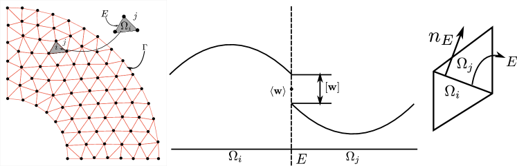
Figure 2: Left: 2D-simplicial mesh. Right: 1D-example of average and jump operators. Interface $E$ between $i$-th and $j$-th cell ($j>i$) is depicted with the used notation. Orientation of outward normal is from lower to higher numbered cell.

Let $\mathcal{F}_{h}^{i}$ be the set of all the interior interfaces $E\subseteq\Omega$ and define the upwind form

$$S_{h}(t;\mathbf{M},\mathbf{N})\mathrel{\mathop{\mathchar 58\relax}}= \sum_{E\in\mathcal{F}_{h}^{i}}\int_{E}\bigg{(}-(\mathbf{u}\cdot\mathbf{n}_{E})[\mathbf{M}]\cdot\left\langle\mathbf{N}\right\rangle+\frac{1}{2}\mathinner{\!\left\lvert\mathbf{u}\cdot\mathbf{n}_{E}\right\rvert}[\mathbf{M}]\cdot[\mathbf{N}]\bigg{)}\;\operatorname{d\!}{s}.$$ (3.3)

Moreover, gradient jumps over interior faces are penalized via

$$p_{\epsilon}(\mathbf{M},\mathbf{N})\mathrel{\mathop{\mathchar 58\relax}}={\tilde{\epsilon}}\sum_{E\in\mathcal{F}_{h}^{i}}h_{E}^{2}\int_{E}|\mathbf{u}\cdot\mathbf{n}_{E}|[\nabla\mathbf{M}]_{E}\mathrel{\mathop{\mathchar 58\relax}}[\nabla\mathbf{N}]_{E}\;\operatorname{d\!}{s},\quad{\tilde{\epsilon}}\geq 0.$$ (3.4)

Setting

$$a_{\epsilon}^{\textnormal{upw}}(t;\mathbf{M},\mathbf{N})\mathrel{\mathop{\mathchar 58\relax}}=p_{\epsilon}(\mathbf{M},\mathbf{N})+a(t;\mathbf{M},\mathbf{N})+S_{h}(t;\mathbf{M},\mathbf{N}),$$ (3.5)

the upwind dG-FEM reads: find $\mathbf{M}_{h}\mathrel{\mathop{\mathchar 58\relax}}(0,T]\mapsto\mathbf{X}_{h}$ such that $\forall\;\mathbf{N}_{h}\in\mathbf{X}_{h}$

$$(\partial_{t}\mathbf{M}_{h},\mathbf{N}_{h})_{\mathbf{H}}+a_{\epsilon}^{\textnormal{upw}}(t;\mathbf{M}_{h},\mathbf{N}_{h})=l(\mathbf{N}_{h}).$$ (3.6)

3.2 Well-posedness of the Semi-discrete Problem

Let us define the norm $\mathopen{|\mkern-1.5mu|\mkern-1.5mu|}\mathbf{N}_{h}\mathclose{|\mkern-1.5mu|\mkern-1.5mu|}_{\mathbf{U}}$ via

$$\mathopen{|\mkern-1.5mu|\mkern-1.5mu|}\mathbf{N}_{h}\mathclose{|\mkern-1.5mu|\mkern-1.5mu|}_{\mathbf{U}}^{2} \mathrel{\mathop{\mathchar 58\relax}}={\tilde{\epsilon}}\sum_{E\in\mathcal{F}_{h}^{i}}h_{E}^{2}\int_{E}|\mathbf{u}\cdot\mathbf{n}_{E}|\mathinner{\!\left\lVert[\nabla\mathbf{N}_{h}]_{E}\right\rVert}^{2}_{L^{2}(E)}$$

$$+\frac{1}{2}\int_{\Gamma}\mathinner{\!\left\lvert\mathbf{u}\cdot\mathbf{n}\right\rvert}\mathinner{\!\left\lvert\mathbf{N}_{h}\right\rvert}^{2}\operatorname{d\!}{s}+\frac{1}{2}\sum_{E\in\mathcal{F}_{h}^{i}}\int_{E}\mathinner{\!\left\lvert\mathbf{u}\cdot\mathbf{n}_{E}\right\rvert}[\mathbf{N}_{h}]_{E}^{2}\operatorname{d\!}{s}.$$ (3.7)

Theorem 3.1.

The semi-discrete problem  3.6 is well-posed and admits the a-priori estimate

$$\frac{1}{2}\mathinner{\!\left\lVert\mathbf{M}_{h}(t)\right\rVert}_{\mathbf{H}}^{2}+\int_{0}^{t}e^{\sigma(\tau-t)}\mathopen{|\mkern-1.5mu|\mkern-1.5mu|}\mathbf{M}_{h}(\tau)\mathclose{|\mkern-1.5mu|\mkern-1.5mu|}_{\mathbf{U}}^{2}\operatorname{d\!}{\tau}\leq\frac{1}{2}\mathinner{\!\left\lVert\mathbf{M}_{h}(0)\right\rVert}_{\mathbf{H}}^{2}e^{-\sigma t}+\frac{1}{2\sigma}\int_{0}^{t}e^{\sigma(\tau-t)}\mathinner{\!\left\lVert\mathbf{f}(\tau)\right\rVert}_{\mathbf{H}}^{2}\operatorname{d\!}{\tau}.$$ (3.8)

Proof.

The existence and uniqueness proof follows the lines of the proof of Theorem 2.1. Similiar to the approach in Sec. 2, symmetric testing $\mathbf{N}_{h}=\mathbf{M}_{h}$ provides

$$a_{\epsilon}^{\textnormal{upw}}((t;\mathbf{M}_{h},\mathbf{M}_{h}) \geq\sigma\mathinner{\!\left\lVert\mathbf{M}_{h}\right\rVert}_{\mathbf{H}}^{2}+\mathopen{|\mkern-1.5mu|\mkern-1.5mu|}\mathbf{M}_{h}\mathclose{|\mkern-1.5mu|\mkern-1.5mu|}^{2}_{\mathbf{U}}.$$ (3.9)

Then, Young inequality shows

$$\frac{1}{2}\mathinner{\dfrac{\operatorname{d\!}{}}{\operatorname{d\!}{t}}}\mathinner{\!\left\lVert\mathbf{M}_{h}(t)\right\rVert}_{\mathbf{H}}^{2}+\frac{\sigma}{2}\mathinner{\!\left\lVert\mathbf{M}_{h}\right\rVert}_{\mathbf{H}}^{2}+\mathopen{|\mkern-1.5mu|\mkern-1.5mu|}\mathbf{M}_{h}\mathclose{|\mkern-1.5mu|\mkern-1.5mu|}_{\mathbf{U}}^{2}\leq\frac{1}{2\sigma}\mathinner{\!\left\lVert f\right\rVert}_{\mathbf{H}}^{2}.$$

Now, similarly to Theorem 2.2, application of the Gronwall lemma yields the a-priori estimate (3.8). This shows the well-posedness of the semi-discretized Bloch problem. ∎

3.3 Semi-discrete Error Estimate

For the error of the spatial discretization we obtain the following result.

Theorem 3.2.

The error of spatial discretization is given by:

$$\frac{1}{2}\mathinner{\!\left\lVert(\mathbf{M}-\mathbf{M}_{h})(t))\right\rVert}_{\mathbf{H}}^{2}+\frac{1}{2}\int_{0}^{t}{\mathrm{e}}^{\sigma(\tau-t)}\mathopen{|\mkern-1.5mu|\mkern-1.5mu|}(\mathbf{M}-\mathbf{M}_{h})(\tau)\mathclose{|\mkern-1.5mu|\mkern-1.5mu|}_{\mathbf{U}}^{2}\operatorname{d\!}{\tau}\leq\frac{1}{2}\mathinner{\!\left\lVert(\mathbf{M}-\mathbf{M}_{h})(0)\right\rVert}_{\mathbf{H}}^{2}{\mathrm{e}}^{-\sigma t}$$

$$+\int_{0}^{t}{\mathrm{e}}^{\sigma(\tau-t)}\Big{(}{\mathopen{|\mkern-1.5mu|\mkern-1.5mu|}(\mathbf{M}-\mathbf{\pi}_{h}\mathbf{M})(\tau)\mathclose{|\mkern-1.5mu|\mkern-1.5mu|}^{2}_{\mathbf{U},\flat}}+\delta\mathinner{\!\left\lVert(\mathbf{M}-\mathbf{\pi}_{h}\mathbf{M})(\tau)\right\rVert}_{\mathbf{H}}+p_{\epsilon}(\mathbf{M},\mathbf{M})(\tau)\Big{)}\operatorname{d\!}{\tau}$$ (3.10)

with the $L^{2}$-orthogonal projection $\mathbf{\pi}_{h}\mathbf{M}$ of $\mathbf{M}$ onto $\mathbf{X}_{h}$ and $\sigma=\frac{1}{T_{1}}$. The norm $\mathopen{|\mkern-1.5mu|\mkern-1.5mu|}\cdot\mathclose{|\mkern-1.5mu|\mkern-1.5mu|}_{U,\flat}$ and constant $\delta$ will be defined within the proof. For a sufficiently smooth solution $\mathbf{M}\in L^{\infty}(0,T;[W^{k+1,2}(\Omega)]^{3})$, the right-hand side term in (3.10) is of order $\mathop{}\!O{\left(h^{2k+1}\right)}$ with $h=\max_{i}\textnormal{diam}(\Omega_{i})$.

Proof.

The error equation for the error $\mathbf{M}-\mathbf{M}_{h}$ is given by

$$(\partial_{t}(\mathbf{M}-\mathbf{M}_{h}),\mathbf{N}_{h})_{\mathbf{H}}+a^{upw}_{\epsilon}(t;\mathbf{M}-\mathbf{M}_{h},\mathbf{N}_{h})=p_{\epsilon}(\mathbf{M},\mathbf{N}_{h})\quad\forall\;\mathbf{N}_{h}\in\mathbf{X_{h}},\leavevmode\nobreak\ t\in(0,T]\leavevmode\nobreak\ \mbox{a.e.}.$$

Let $\pi_{h}\mathbf{N}$ be the $L^{2}$-orthogonal projection of $\mathbf{N}$ onto $\mathbf{X}_{h}$, i.e., $(\mathbf{N}-\pi_{h}\mathbf{N},\mathbf{w})_{\mathbf{H}}=0\quad\forall\;\mathbf{w}\in\mathbf{X}_{h}.$ Then we split the error as

$$\mathbf{M}-\mathbf{M}_{h}=(\mathbf{M}-\mathbf{\pi}_{h}\mathbf{M})+(\mathbf{\pi}_{h}\mathbf{M}-\mathbf{M}_{h})\equiv\mathbf{I}_{h}+\mathbf{E}_{h}$$

and reformulate the error equation with $\mathbf{N}_{h}=\mathbf{E}_{h}$ as

$$(\partial_{t}\mathbf{E}_{h},\mathbf{E}_{h})_{\mathbf{H}}+a^{upw}_{\epsilon}(t;\mathbf{E}_{h},\mathbf{E}_{h})=-a^{upw}_{\epsilon}(t;\mathbf{I}_{h},\mathbf{E}_{h})+p_{\epsilon}(\mathbf{M},\mathbf{E}_{h}),\quad t\in(0,T]\leavevmode\nobreak\ \mbox{a.e.}$$ (3.11)

where we used that $(\partial_{t}\mathbf{I}_{h},\mathbf{E}_{h})_{\mathbf{H}}=0$ due to $L^{2}$-orthogonality. The left-hand side can be bounded from below as

$$(\partial_{t}\mathbf{E}_{h},\mathbf{E}_{h})_{\mathbf{H}}+a^{upw}_{\epsilon}(t;\mathbf{E}_{h},\mathbf{E}_{h})\geq\frac{1}{2}\frac{d}{dt}\mathinner{\!\left\lVert\mathbf{E}_{h}\right\rVert}^{2}_{\mathbf{H}}+\sigma\mathinner{\!\left\lVert\mathbf{E}_{h}\right\rVert}^{2}_{\mathbf{H}}+\mathopen{|\mkern-1.5mu|\mkern-1.5mu|}\mathbf{E}_{h}\mathclose{|\mkern-1.5mu|\mkern-1.5mu|}_{\mathbf{U}}^{2}.$$ (3.12)

For an estimate of the right-hand side we use $p_{\epsilon}(\mathbf{M},\mathbf{E}_{h})\leq p_{\epsilon}(\mathbf{M},\mathbf{M})\mathopen{|\mkern-1.5mu|\mkern-1.5mu|}\mathbf{E}_{h}\mathclose{|\mkern-1.5mu|\mkern-1.5mu|}_{\mathbf{U}}$ and

$$-a^{upw}_{\epsilon}(t;\mathbf{I}_{h},\mathbf{E}_{h})\leq\Big{(}{\mathopen{|\mkern-1.5mu|\mkern-1.5mu|}\mathbf{I}_{h}\mathclose{|\mkern-1.5mu|\mkern-1.5mu|}_{\mathbf{U},\flat}}+\delta\mathinner{\!\left\lVert\mathbf{I}_{h}\right\rVert}^{2}_{\mathbf{H}}\Big{)}\mathopen{|\mkern-1.5mu|\mkern-1.5mu|}\mathbf{E}_{h}\mathclose{|\mkern-1.5mu|\mkern-1.5mu|}_{\mathbf{U}}$$ (3.13)

with

$${\mathopen{|\mkern-1.5mu|\mkern-1.5mu|}\mathbf{I}_{h}\mathclose{|\mkern-1.5mu|\mkern-1.5mu|}^{2}_{\mathbf{U},\flat}}\mathrel{\mathop{\mathchar 58\relax}}=\zeta\mathopen{|\mkern-1.5mu|\mkern-1.5mu|}\mathbf{I}_{h}\mathclose{|\mkern-1.5mu|\mkern-1.5mu|}^{2}_{\mathbf{U}}+\sum_{T\in\mathcal{T}_{h}}\mathinner{\!\left\lVert\mathbf{u}\right\rVert}_{L^{\infty}(\partial T)}\mathinner{\!\left\lVert\mathbf{I}_{h}\right\rVert}^{2}_{L^{2}(\partial T)}$$ (3.14)

and $\delta\mathrel{\mathop{\mathchar 58\relax}}=\gamma\mathinner{\!\left\lVert\mathbf{B}\right\rVert}_{L^{\infty}}+\mathinner{\!\left\lVert D\right\rVert}_{L^{\infty}}$ resp. $\zeta\mathrel{\mathop{\mathchar 58\relax}}=\max\{1;\mathinner{\!\left\lVert\mathbf{u}\right\rVert}_{L^{\infty}(0,T;W^{1,\infty}(\Omega))}\}.$ Estimate (3.13) relies on a generalization of Lemma 2.30 in [14] for scalar advection-reaction problems to the vector-valued case. The estimate provides a careful bound of the uwpind-discretized convective term and heavily exploits the boundedness of $L^{2}$-orthogonality of subscales.

Combining (3.12), (3.13) and using Young inequality, we obtain

$$\frac{1}{2}\frac{d}{dt}\mathinner{\!\left\lVert\mathbf{E}_{h}\right\rVert}^{2}_{\mathbf{H}}+\frac{1}{2}\mathopen{|\mkern-1.5mu|\mkern-1.5mu|}\mathbf{E}_{h}\mathclose{|\mkern-1.5mu|\mkern-1.5mu|}_{\mathbf{U}}^{2}\leq\mathopen{|\mkern-1.5mu|\mkern-1.5mu|}\mathbf{I}_{h}\mathclose{|\mkern-1.5mu|\mkern-1.5mu|}^{2}_{\mathbf{U},\flat}+\delta\mathinner{\!\left\lVert\mathbf{I}_{h}\right\rVert}^{2}_{\mathbf{H}}+p_{\epsilon}(\mathbf{M},\mathbf{M}).$$ (3.15)

Integration of (3.15) and the triangle inequality imply the quasi-optimal error estimate (3.10). For a sufficiently smooth solution $\mathbf{M}\in L^{\infty}(0,T;[W^{k+1,2}(\Omega)]^{3})$, the penalty term $p_{\epsilon}(\mathbf{M},\mathbf{M})$ vanishes. Finally, interpolation results imply the error order $\mathop{}\!O{\left(h^{k+\nicefrac{{1}}{{2}}}\right)}$. ∎

Remark.

The case $k=0$ covers the finite volume method (FVM).

4 Temporal Discretization

Starting point is the spatially discretized problem: find $\mathbf{M}_{h}\mathrel{\mathop{\mathchar 58\relax}}(0,T]\mapsto\mathbf{X}_{h}$ such that for all $\mathbf{N}_{h}\in\mathbf{X}_{h}$

$$(\partial_{t}\mathbf{M}_{h}(t),\mathbf{N}_{h})_{\mathbf{H}}+a_{\epsilon}^{\textnormal{upw}}(t;\mathbf{M}_{h}(t),\mathbf{N}_{h})=l(\mathbf{N}_{h}),\quad\mathbf{M}_{h}(0)=\mathbf{M}_{h0}.$$ (4.1)

A major problem stems from the multiscale character of 4.1 as the scale of magnetization is much faster than that of advection. Another difficulty is the restricted smoothness of the data in time, in particular of field $\mathbf{G}=\begin{pmatrix}G_{x},G_{y},G_{z}\end{pmatrix}^{T}$, see Fig. 3 (for the FLASH sequence [16, 17]).

According to the required high resolution in time, an explicit time stepping is chosen. We considered two variants (i) a fully coupled approach and (ii) an operator splitting approach. The efficiency of the numerical simulation can be strongly improved using GPU computing. This will be exemplarily shown in Sec. 5.

4.1 Fully Coupled Approach

Following Sec. ($3.1$) in [14], we apply a low-order explicit Runge-Kutta scheme to 4.1. Define a discrete operator $A_{\epsilon}^{\textnormal{upw}}\mathrel{\mathop{\mathchar 58\relax}}\mathbf{X}+\mathbf{X}_{h}\mapsto\mathbf{X}_{h}$ via $(A_{\epsilon}^{\textnormal{upw}}(t)\mathbf{v},\mathbf{w})_{\mathbf{H}}\mathrel{\mathop{\mathchar 58\relax}}=a_{\epsilon}^{\textnormal{upw}}(t;\mathbf{v},\mathbf{w})$. Similarly, let $L$ be a functional on $\mathbf{X}_{h}$ with $L=l(\mathbf{w})$. Note that $L$ is constant in time in this application.

Let $0=t^{0}<t^{1}<t^{2}<\cdots<t^{N}=T$ be the set of discrete times with time steps $\tau_{n}\mathrel{\mathop{\mathchar 58\relax}}=t^{n+1}-t^{n},n=0,1,\cdots,N-1$. Moreover, we denote $\mathbf{M}_{h}^{n}=\mathbf{M}_{h}(t^{n})$ etc.

A two-stage RK-scheme is a good compromise between temporal accuracy and the restricted data smoothness in time. Following Subsec. 3.1.3 in [14] we select scheme

$$\mathbf{M}_{h}^{n,1} =\mathbf{M}_{h}^{n}-\tau_{n}A_{\epsilon}^{\textnormal{upw}}\mathbf{M}_{h}^{n}+\tau_{n}L$$ (4.2a)

$$\mathbf{M}_{h}^{n+1} =\frac{1}{2}(\mathbf{M}_{h}^{n}+\mathbf{M}_{h}^{n,1})-\frac{1}{2}\tau_{n}A_{\epsilon}^{\textnormal{upw}}\mathbf{M}_{h}^{n,1}+\frac{1}{2}\tau_{n}L.$$ (4.2b)

Precise statements of the stability and convergence of 4.2a can be found in case of smooth data in Subsec. 3.1.6 of [14]. In particular, a time step restriction on $\tau_{n}$ comes from a CFL condition for the advective term. As in this application the time step restriction on $\tau_{n}$ comes from magnetization, the mentioned CFL condition is always valid in our calculations.

We will not repeat the details, e.g. of the stability and convergence RK2-analysis in [14]. It provides in case of smooth data in time, an error of order $\mathop{}\!O{\left(\tau_{n}^{2}+h^{k+\nicefrac{{1}}{{2}}}\right)}$ with polynomial degree $k$ of spatial discretization (see Theorem 3.10). Such error estimate in time is not valid in this application, since the data $\mathbf{B}(t,\mathbf{r})$ are only in $[C^{0,1}[0,T]]^{3}$ (for the FLASH-sequence studied in Sec. 5) or even only in $[L^{\infty}(0,T)]^{3}$ for the example in Subsec. 5.2. Alternatively, a standard embedded RK-scheme of type RK3(2) or even of higher order like RK5(4) is chosen for appropriate time step selection, see Sec. 5. For details of the embedded methods, we refer, e.g., to Sec. 5 of [18].

4.2 Operator Splitting

The above mentioned multiscale character of problem 4.1 suggests an operator splitting approach as suggested e.g.in Sec. IV.1.5. of [19] for large advection-reaction problems, e.g. in air-pollution simulations. Writing the semi-discrete problem 4.1 with

$$\mathbf{F}_{\textnormal{adv}}(t,\mathbf{M})\mathrel{\mathop{\mathchar 58\relax}}=-\nabla\cdot(\mathbf{u}\mathbf{M}),\quad\mathbf{F}_{\textnormal{mag}}\mathrel{\mathop{\mathchar 58\relax}}=\gamma\mathbf{B}\times\mathbf{M}+D\mathbf{M}-\mathbf{f},$$ (4.3)

formally as ODE-system

$$\mathinner{\dfrac{\operatorname{d\!}{}\mathbf{M}_{h}(t)}{\operatorname{d\!}{t}}}=\mathbf{F}_{\textnormal{adv}}(t,\mathbf{M}_{h}(t))+\mathbf{F}_{\textnormal{mag}}(t,\mathbf{M}_{h}(t)),$$ (4.4)

the simplest sequential operator splitting on $t^{n}\leq t\leq t^{n+1}$ gives

$$\mathinner{\dfrac{\operatorname{d\!}{}\mathbf{M}_{h}^{*}(t)}{\operatorname{d\!}{t}}} =\mathbf{F}_{\textnormal{adv}}(t,\mathbf{M}_{h}^{*}(t)), \mathbf{M}_{h}^{*}(t)=\mathbf{M}_{h}(t^{n}),$$ (4.5a)

$$\mathinner{\dfrac{\operatorname{d\!}{}\mathbf{M}_{h}^{**}(t)}{\operatorname{d\!}{t}}} =\mathbf{F}_{\textnormal{mag}}(t,\mathbf{M}_{h}^{**}(t)), \mathbf{M}_{h}^{**}(t)=\mathbf{M}_{h}^{*}(t^{n}).$$ (4.5b)

An inspection of 4.5 shows for the splitting error at $t=t^{n}$

$$\bm{\epsilon}_{s}=\frac{1}{2}\tau_{n}^{2}[\mathinner{\dfrac{\partial{}\mathbf{F}_{\textnormal{adv}}}{\partial{\mathbf{M}}}}\mathbf{F}_{\textnormal{mag}}-\mathinner{\dfrac{\partial{}\mathbf{F}_{\textnormal{mag}}}{\partial{\mathbf{M}}}}\mathbf{F}_{\textnormal{adv}}]+\mathop{}\!O{\left(\tau_{n}^{3}\right)}.$$ (4.6)

It turns out that the commutation error $[\mathbf{F}_{\textnormal{adv}},\mathbf{F}_{\textnormal{mag}}]=\mathinner{\dfrac{\partial{}\mathbf{F}_{\textnormal{adv}}}{\partial{\mathbf{M}_{h}}}}\mathbf{F}_{\textnormal{mag}}-\mathinner{\dfrac{\partial{}\mathbf{F}_{\textnormal{mag}}}{\partial{\mathbf{M}_{h}}}}\mathbf{F}_{\textnormal{adv}}$ can be written as

$$[\mathbf{F}_{\textnormal{adv}},\mathbf{F}_{\textnormal{mag}}]=(\nabla\cdot\mathbf{u})[\mathbf{F}_{\textnormal{mag}}(t,\mathbf{M}_{h})-\mathinner{\dfrac{\partial{}\mathbf{F}_{\textnormal{mag}}}{\partial{t}}}(t,\mathbf{M}_{h})\mathbf{M}_{h}(t)]+(\mathbf{u}\cdot\nabla_{\mathbf{r}})\mathbf{F}_{\textnormal{mag}}(t,\mathbf{M}_{h}).$$ (4.7)

It vanishes if either $\mathbf{F}_{\textnormal{mag}}$ is independent of $\mathbf{r}=(x,y,z)^{T}$ and $\mbox{div}\leavevmode\nobreak\ \mathbf{u}=0$ or $\mathbf{F}_{\textnormal{mag}}$ is independent of $\mathbf{r}$ and linear in $\mathbf{M}_{h}$, see [19], sec IV.1.5. This is unfortunately not the case in this application. As a remedy, symmetric or Strang-Marchuk splitting can be applied which reduces the splitting error to $\mathop{}\!O{\left(\tau_{n}^{2}\right)}$, see [19].

5 Numerical Experiments

The simulation method was tested for both static objects, i.e. with $\mathbf{u}\equiv\mathbf{0}$, as well as flow experiments, i.e. with $\mathbf{u}\not\equiv\mathbf{0}$.

5.1 Experimental Validation for Static Objects ($\mathbf{u}\equiv\mathbf{0}$)

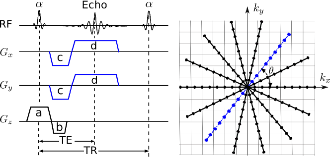
Figure 3: Generic spoiled gradient echo sequence with radial trajectory. Gradients: (a) slice selection (b) rewinder (c) prephasing (d) readout. The dashed radial line (spoke) in the $\mathbf{k}$-space corresponds to the current repetition.

We start with a test of the simulator for the static case, i.e. for $\mathbf{u}=\mathbf{0}$. This means that mainly the temporal discretization is considered. The experiments here and later on (with exception of Subsec. 5.2) were performed using a randomly spoiled [20] FLASH sequence [16, 17] with a radial trajectory as shown in Fig. 3. The left part depicts the time diagram of gradients and the right part shows the $\mathbf{k}$-space sampling trajectory where

$$k_{x}\mathrel{\mathop{\mathchar 58\relax}}=\frac{\gamma}{2\pi}\int_{0}^{t}G_{x}(\tau)\operatorname{d\!}{\tau},\qquad k_{y}\mathrel{\mathop{\mathchar 58\relax}}=\frac{\gamma}{2\pi}\int_{0}^{t}G_{y}(\tau)\operatorname{d\!}{\tau}$$

with $G_{x}=G_{\textnormal{max}}\cos(\theta)$, $G_{y}=G_{\textnormal{max}}\sin(\theta)$, $G_{\textnormal{max}}=\sqrt{G_{x}^{2}+G_{y}^{2}}$ and angle $\theta$ of the spoke with $x$-axis. Putting the expression of $\mathbf{k}$ in the demodulated signal equation, we can obtain the Fourier pair relation between the acquired electric signal and the transverse magnetization [1]. Each radial spoke in $\mathbf{k}$-space, which represents a projection of the object, is acquired with a repetition of pulse sequence where transverse gradients are changed according to orientation $\theta$ of the spoke in $\mathbf{k}$-space. Certain number of spokes in $\mathbf{k}$-space are required to reconstruct an image frame.

Carr showed in [21] that under constant flip angle $\alpha$, and gradient moment and constant TR the magnetizations reach a state of dynamic equilibrium after several repetitions. For clinical imaging, the acquisition starts only after the magnetizations reach dynamic equilibrium after several preparatory TR repetition. In order to test the simulations, time-series data of images from the beginning of the preparatory phase to dynamic equilibrium were obtained from experiments and compared with equivalent simulation results.

Table 1: Doped water tubes with their relaxation times

Tube	$T_{1}$ [$\mathrm{ms}$]	$T_{2}$ [$\mathrm{ms}$]
3	296	113
4	463	53
7	604	95
10	745	157
14	1034	167
16	1276	204
water	2700	2100

To this end, an experiment was performed with a phantom as can be seen in the left part of Fig. 4) containing multiple compartments of doped water tubes with known $T_{1}$ and $T_{2}$ as listed in Table 1. The relevant pulse sequence parameters in Fig. 3 are: TR/TE = $2.18\text{/}1.28\text{\,}\mathrm{ms}$, flip angle $\alpha$ =$8\mathrm{°}$, and number of spokes per image frame= $27$. $100$ image frames from the beginning to the dynamic equilibrium of the experiment were used for comparison with simulation results.

Before embarking on the validation of our code with experimental results, it was tested with a Bloch equation simulator written in MATLAB by Sun [22] where the computationally expensive parts are written in C and connected via mex interface [22]. The code is an extended and corrected version of the code by Hargreaves [7]. The numerical results from our code agree really well with [22]. Baseline simulations were performed on a system with Supermicro SuperServer 4027GR-TR system with Ubuntu 14.04, 2x Intel Xeon Ivy Bridge E5-2650 main processors using an in-house C++ code and the implementation by Sun in Matlab R2016A. Though computationally RK5(4) solver is $4$ times more expensive, the advantage of using RK5(4) is an easy higher order extension for flowing cases with any method of our choice for spatial discretization and we can avoid splitting error using a fully coupled approach.

Prior studies [23] have shown that, to model Bloch phenomena accurately, simulations must be carried out dividing each voxel with a number of cells where each of them represent one or an ensemble of isochromats; an isochromat is a microscopic group of spins which resonate at the same frequency. Shkarin et. al. showed in that [23] increasing the number of cells per voxel reduce the error of the solution.

For every simulation with relaxation time of specific liquids, the simulated data were recorded at TE since all isochromats are rephased at TE under the condition of approximately complete spoiling of residual transverse magnetization. The transverse magnetizations are integrated over all the isochromats and the magnitude of the summed up transverse magnetizations are averaged further for the number of spokes per image frame. In principle, this averaged integrated transverse magnetization should be equivalent to the averaged magnitude of image over a region in a specific tube.

Simulations were performed over a domain of $4.8\text{\times}4.8\text{\times}18.0\text{\,}\mathrm{mm}$ (corresponding to $3\times 3$ pixels in the $xy$-plane and three-times the nominal slice thickness=$6\text{\,}\mathrm{mm}$ in $z$-direction for each tube) divided into $27\text{\times}27\text{\times}45$ cells. Each cell is assumed to consist of one isochromat as shown in Subsec. 3.4.3. in [24] that the number of isochromats in each cell do not effect accuracy of the simulation. The initial condition is chosen as $\mathbf{M}^{0}=(0,0,1)^{T}$. The embedded RK5(4) scheme is applied for time discretization. The time series of these two equivalent quantities are plotted as a function of image frame number in Fig. 4 (right) for four randomly chosen tubes after normalizing the experimental and simulated data by their respective magnitude in dynamic equilibrium of the brightest tube (Tube 3).

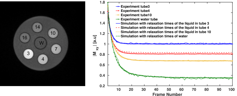
Figure 4: Left: Image of the static phantom with resolution of $160\text{\times}160$ pixels. Right: Comparison of simulation with the image for four different liquids.

The excellent agreement between simulation and experiment hints at the possible use of the simulator for quantitative estimations in MRI, e.g. the relaxation times $T_{1}$, $T_{2}$ or concentration of contrast agents required for certain signal enhancement (illustrated with an example in [24], Sec. 5.4).

Also, the time evolution of magnetizations for different isochromats are independent of each other and suitable for Graphical Processing Unit (GPU) computing. A speed-up of 82 was achieved with GPU parallelization on the previously mentioned system together with a NVIDIA GTX Titan Black (Kepler GK110) GPU as illustrated in Subsec. 3.3.4 of [24].

5.2 A Basically One-dimensional Test Case for Flowing Spins

The simulator is tested further for flowing spins, i.e. $\mathbf{\mathbf{u}}\not\equiv\mathbf{0}$. As first case, we consider a basically one-dimensional test case in [10] where they studied for $z\in(-\frac{L}{2},\frac{L}{2})$ the effect of an RF pulse on the magnetization for different through-plane velocities, i.e. component $u_{z}$ in $z$-direction, using the leap-frog finite difference scheme.

Figure 5: A $90\mathrm{°}$ slice-selective pulse was used for the studying the flow-effects. The arrows indicate the time when the data was recorded.

As shown in Fig. 5, a Blackman-windowed sinc pulse with an amplitude of $0.1750\text{\,}\mathrm{G}$, flip angle of $90\mathrm{°}$ and duration of $2.6794\text{\,}\mathrm{ms}$, slice selection gradient $G_{z}=$1.0\text{\,}\mathrm{G}\text{\,}{\mathrm{cm}}^{-1}$$, and a nominal slice thickness of $7\text{\,}\mathrm{mm}$ were used for the simulation in [10]. Through-plane velocities were in the range of $0200\text{\,}\mathrm{cm}\text{\,}{\mathrm{s}}^{-1}$. The simulations were performed over a length of $L=$20\text{\,}\mathrm{mm}$$ and $L=$30\text{\,}\mathrm{mm}$$, respectively, in the slice direction $z$, divided into $800$ cells of size $0.025\text{\,}\mathrm{mm}$ and $0.0375\text{\,}\mathrm{mm}$ for the range of velocities $080\text{\,}\mathrm{cm}\text{\,}{\mathrm{s}}^{-1}$ and $80200\text{\,}\mathrm{cm}\text{\,}{\mathrm{s}}^{-1}$ respectively. The time duration of simulations was divided into $4500$ equidistant time steps of $\tau_{n}=$8.9313\text{\times}{10}^{-04}\text{\,}\mathrm{ms}$$. The magnetizations were calculated at the end of the rewinder gradient marked by an arrow in Fig. 5

In this work, the simulations were performed with the FEM-package COMSOL Multiphysics using the dG-FEM with quadratic elements ($k=2$), see Sec. 3. The domain of L=$30\text{\,}\mathrm{mm}$ was divided into $200$ equidistant cells for the velocity range $0200\text{\,}\mathrm{cm}\text{\,}{\mathrm{s}}^{-1}$. The fully coupled semi-discretized equations were further solved using the RK5(4) scheme. For relative and absolute tolerance of $1.0\text{\times}{10}^{-6}$ and $1.0\text{\times}{10}^{-8}$ respectively, the adaptive time stepping resulted in $340528$ time steps in the specified velocity range. The variability of time step sizes due to the embedded RK is depicted in Fig. 6 (Left) and the figure also clearly shows sudden reduction in the time step size due to time adaptivity to cater for jump in $G_{z}$. Also, the number of time steps got reduced by an order of magnitude due to time adaptation of the embedded RK scheme.

In order to estimate grid convergence, simulations were performed for $163264128256$ equidistant grid points in z-direction with $u_{z}=$80\text{\,}\mathrm{cm}\text{\,}{\mathrm{s}}^{-1}$$. The solution with the finest grid was chosen as the reference for the estimation of errors for $M_{y}$. Fig. 6 (Right) shows the error order and the results show faster convergence rate than the predicted theoretical estimate.

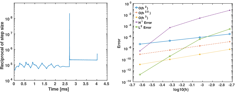
Figure 6: Left: Reciprocal of variable time step size as a function of time duration for $u_{z}=$200\text{\,}\mathrm{cm}\text{\,}{\mathrm{s}}^{-1}$$. Right: Numerical errors estimated with different grid sizes comparing with the reference solution obtained dividing the length in $z$-direction into $256$ grid points and with $u_{z}=$80\text{\,}\mathrm{cm}\text{\,}{\mathrm{s}}^{-1}$$. Different error estimates are plotted in logarithmic scale as a function of logarithm of grid sizes.

The penalty diffusion term $p_{\epsilon}$ with constant $\tilde{\epsilon}=$5.0\text{\times}{10}^{-04}$$ was used to remove unphysical oscillations appearing in the neighborhood of inflow boundary for $M_{x}$ and $M_{y}$. Such oscillations for $M_{y}$ are shown in Fig. 7. Similar oscillations were observed for $M_{x}$ but not for $M_{z}$.

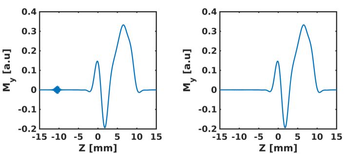
Figure 7: Simulation for $u_{z}=$160\text{\,}\mathrm{cm}\text{\,}{\mathrm{s}}^{-1}$$. Left: with $\epsilon=0$ results in unphysical oscillations in the neighborhood of inflow boundary for $M_{y}$. Right: Unphysical oscillations vanish after the introduction of a small artificial diffusion term with $\tilde{\epsilon}=$5.0\text{\times}{10}^{-4}$$.

Finally, the results are compared with [10] and they show extremely good agreement. The effect of velocity $u_{z}$ in the range $0200\text{\,}\mathrm{cm}\text{\,}{\mathrm{s}}^{-1}$ on magnetization is shown in Fig. 8.

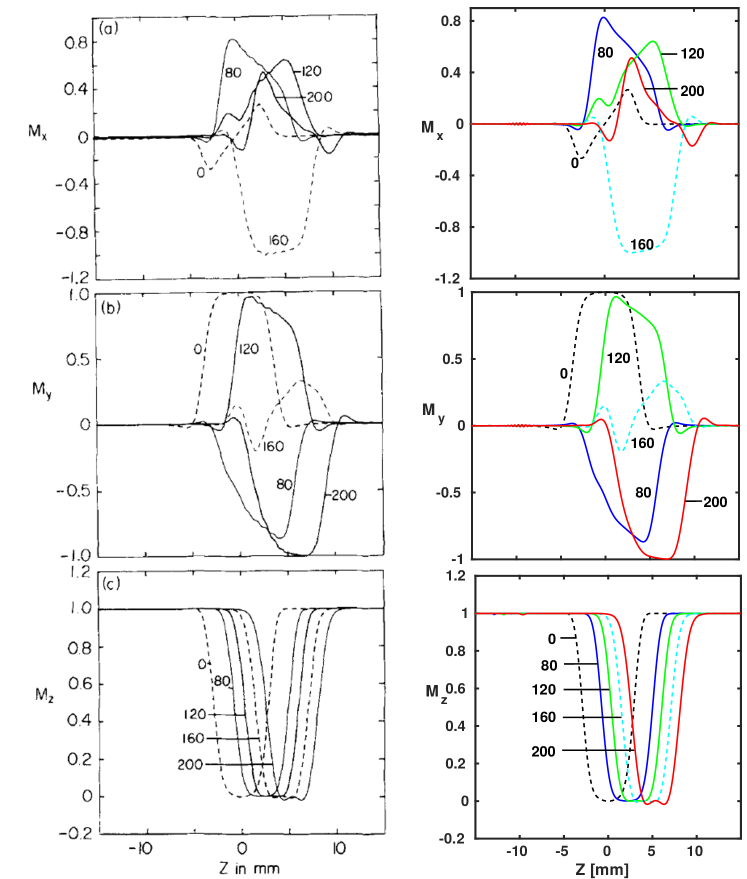
Figure 8: Simulated magnetization distributions of $M_{x}$, $M_{y}$, $M_{z}$ for through-plane velocity $u_{z}$ along the positive $z$-axis in the range $0200\text{\,}\mathrm{cm}\text{\,}{\mathrm{s}}^{-1}$ using dG-method (right) are compared with the results in [10] (Left). The magnetizations were recorded at the end of rewinder gradient as marked by the arrow Fig. 5. The length in the slice direction is in the range $-1515\text{\,}\mathrm{mm}$.

5.3 Comparison with Experiments for Through-plane Flow

The simulator was evaluated further against a laminar flow experiment in a circular tube. In the experiment, the flow pump was operated at different voltages to produce velocities such that the flow profile could be expected to be laminar i.e. Reynolds number $Re\leq 2300$ as listed in Table 2.

The flow velocities were estimated pixelwise using phase contrast MRI (PC MRI) [25]. At each listed operating voltage in Table 2, the mean through-plane flow velocity $u_{z}$ was calculated over a pixel. The measured velocities show an unsteady pattern with a mean and a standard deviation as listed in the second and the third column of Table 2.

Table 2: Mean and standard deviation velocities and $Re$ based on the mean velocity for different operating voltages of the flow pump at temperature $16\text{\,}\mathrm{\SIUnitSymbolCelsius}$ (kinematic viscosity $\nu=$1.1092\text{\times}{10}^{-02}\text{\,}\mathrm{c}\mathrm{m}^{2}\mathrm{/}\mathrm{s}$$).

Voltage [$\mathrm{V}$]	Mean Velocity [$\mathrm{mm}\text{\,}{\mathrm{s}}^{-1}$]	Standard Deviation [$\mathrm{mm}\text{\,}{\mathrm{s}}^{-1}$]	$Re$
6	49.19	2.26	2217
5	38.71	1.97	1744
4	28.84	1.47	1300
3	18.52	1.04	834

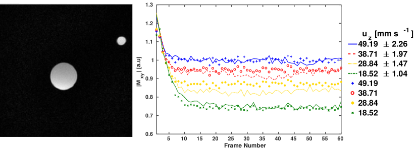
Figure 9: Left: MR image of the flow tube. Right: Experiments with different velocities are compared with the simulations.

At each specified flow velocity $u_{z}$, measurements were performed with the FLASH pulse sequence parameters TR/TE = $1.96\text{/}1.22\text{\,}\mathrm{ms}$, flip angle = $8\mathrm{°}$, and number of spokes per image frame = $17$. The resolution of one pixel in the $xy$-plane is $1.6\text{\times}1.6\text{\,}\mathrm{mm}$ whereas the nominal slice thickness in $z$-direction is $6\text{\,}\mathrm{mm}$. The time series of averaged magnitude is recorded over the same region of interest as the region of flow velocity measurement. $60$ frames from the beginning of experiments towards dynamic equilibrium were used for the comparison with simulation.

The mean velocity $\mathbf{u}=(0,0,u_{z})^{T}$ was taken as input velocity in the simulation. A computational domain of $1.6\text{\times}1.6\text{\times}18.0\text{\,}\mathrm{mm}$, divided into $6\text{\times}6\text{\times}27$ identical cells, was chosen for the simulation. The length of domain in the through-plane flow direction was estimated from previous simulation results [24] such that $\mathbf{M}_{\Gamma_{-}}=(0,0,1)^{T}$, i.e. the Dirichlet inflow boundary condition, could be satisfied. The initial condition was chosen as in the static case. The spatial discretization was performed using dG-FEM with quadratic elements ($k=2$) whereas in time the fully coupled approach with the RK5(4)-scheme for time discretization was applied. Again the penalty diffusion term $p_{\epsilon}$ with constant $\epsilon=$5.0\text{\times}{10}^{-04}$$ was used.

For comparison, the experimental and simulated data are normalized properly first. Due to unsteadiness of the flow, the experimental data was normalized by the average magnitude of last $20$ frames from the measurement with the operating voltage of $6\text{\,}\mathrm{V}$ in Table 2. The simulated data was normalized similarly. After that, they are plotted in the right part of Fig. 9.

In spite of the unsteadiness in the flow which may be attributed to the lack of sufficient entry length, as discussed in [24], the simulation and the experiment show a reasonable agreement.

Like the static phantom, GPU computing can be used for the flowing fluid as well to achieve a significant speed up as explained in Subsec. 4.4.3 of [24].

5.4 Comparison with Pulsatile Flow Experiments

The simulation method was evaluated further with a pulsatile flow laboratory experiment. Like in the previous case, the pulsatile velocity profile was estimated using PC MRI. A through-plane profile was fitted as a function of time using Matlab curve-fitting toolbox as shown in the left part of Fig. 10. The fitted pulsatile flow profile was used as input velocity in the simulation. The effect of pulsatile flow on the evolution of magnitude from the image was studied. An experiment was performed using the pulse sequence identical to the previous experiment.

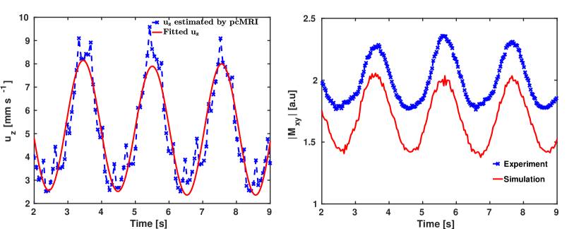
Figure 10: Left: Fitted through-plane velocity profile from PC MRI data. Right: Comparison between experimental and simulation results for studying the effect of pulsatile flow.

The simulation was performed with identical domain, spatial and temporal discretization, and penalty diffusion as used in the previous experiment. Experimental data was normalized with the magnitude data in dynamic equilibrium from the spatially stationary tube under identical experimental conditions. The simulated data was normalized by the averaged magnitude of integrated transverse magnetization of static water in dynamic equilibrium. The experiment and the simulation are compared in a state of dynamic equilibrium in Fig. 10 (right).

Fig. 10 shows that, although the periodicity in the experimental and the simulated result agree well, the amplitude of experimental results deviates from the simulation. The deviation could be due to the assumption of a flow profile which depends only on time. The assumption implies that the fluid needs to move in bulk, i.e., the tube must respond simultaneously to the changing pressure at all positions at every specific point of time in the direction of through-plane flow such that through-plane velocities at every position in the longitudinal direction are same, which is artificial and unphysical. Nevertheless, it is a starting point to study the effect of more realistic pulsatile flows.

6 Summary. Outlook

In this note, we proved the well-posedness of the Bloch model under the action of an incompressible flow field. Then we applied the discontinuous Galerkin method to the spatial semi-discretization of the Bloch model and proved well-posedness and error estimates. The multiscale character of the problem basically stems from the high frequency time evolution of the magnetization part. An explicit Runge-Kutta method together with time step adaption is applied for the temporal discretization. Alternatively, an operator splitting between advection and magnetization can be applied. The computation can be strongly accelerated via GPU computing.

Magnetic resonance imaging is nowadays a very rapid process which can be done in real-time [26]. Nevertheless, there are still unsolved problems such as a quantitative understanding of the mechanisms that lead to MRI signal alterations (i.e., both enhancement and loss) when imaging flowing spins (e.g., in vessels or the heart) or other dynamic processes. Here, numerical simulation with the proposed direct solver for the Bloch model can help in a better understanding of such dynamic processes as shown for some basic MRI experiments. Apart from flow velocities and volumes, there is an increasing demand in MRI for quantitative information such as relaxation time constants. In future, access to both high-contrast imaging and quantitative parametric mapping by MRI is expected to facilitate and contribute to computer-aided diagnostic strategies.

References

- [1] D. G. Nishimura, Principles of magnetic resonance imaging, Stanford University, 1996.
- [2] F. Bloch, Nuclear induction, Physical Review 70 (7-8) (1946) 460–474.
- [3] E. O. Stejskal, J. E. Tanner, Spin diffusion measurements: spin echoes in the presence of a time-dependant field gradient, The Journal of chemical physics 42 (1) (1965) 288–292.
- [4] S. Lorthois, J. Stroud-Rossman, S. Berger, L. D. Jou, D. Saloner, Numerical simulation of magnetic resonance angiographies of an anatomically realistic stenotic carotid bifurcation, Annals of Biomedical Engineering 33 (3) (2005) 270–283.
- [5] J. Bittoun, J. Taquin, M. Sauzade, A computer algorithm for the simulation of any Nuclear Magnetic Resonance (NMR) imaging method, Magnetic Resonance Imaging 2 (2) (1984) 113–120.
- [6] T. Stöcker, K. Vahedipour, D. Pflugfelder, N. J. Shah, High-performance computing MRI simulations, Magnetic Resonance in Medicine 64 (1) (2010) 186–193. doi:10.1002/mrm.22406.
- [7] B. Hargreaves, Bloch equation simulator, http://mrsrl.stanford.edu/~brian/blochsim/, published January 13, 2004.
- [8] H. Benoit-Cattin, G. Collewet, B. Belaroussi, H. Saint-Jalmes, C. Odet, The SIMRI project: A versatile and interactive MRI simulator, Journal of Magnetic Resonance 173 (1) (2005) 97–115.
- [9] C. G. Xanthis, I. E. Venetis, A. V. Chalkias, A. H. Aletras, MRISIMUL: A GPU-based parallel approach to MRI simulations, IEEE Transactions on Medical Imaging 33 (3) (2014) 607–617.
- [10] C. Yuan, G. T. Gullberg, D. L. Parker, The solution of bloch equations for flowing spins during a selective pulse using a finite difference method, Medical physics 14 (6) (1987) 914–921.
- [11] L. D. Jou, R. van Tyen, S. A. Berger, D. Saloner, Calculation of the magnetization distribution for fluid flow in curved vessels, Magnetic Resonance in Medicine 35 (4) (1996) 577–584.
- [12] K. Jurczuk, M. Kretowski, J. J. Bellanger, P. A. Eliat, H. Saint-Jalmes, J. Bézy-Wendling, Computational modeling of MR flow imaging by the lattice Boltzmann method and Bloch equation, Magnetic Resonance Imaging 31 (7) (2013) 1163–1173.
- [13] A. Ern, J.-L. Guermond, Theory and practice of finite elements, Vol. 159, Springer Science & Business Media, 2004.
- [14] D. A. Di Pietro, A. Ern, Mathematical aspects of discontinuous Galerkin methods, Vol. 69, Springer Science & Business Media, 2011.
- [15] J. L. Lions, Perturbations singulières dans les problèmes aux limites et en contrôle optimal, Vol. 323, Springer, 2006.
- [16] J. Frahm, A. Haase, D. Matthaei, W. Hänicke, K.-D. Merboldt, Verfahren und Einrichtung zur schnellen Akquisition von Spinresonanzdaten für eine ortsaufgelöste Untersuchung eines Objekts (1985).
- [17] A. Haase, J. Frahm, D. Matthaei, W. Hanicke, K.-D. Merboldt, FLASH imaging. Rapid NMR imaging using low flip-angle pulses, Journal of Magnetic Resonance 67 (2) (1986) 258–266.
- [18] P. Deuflhard, F. Bornemann, Scientific computing with ordinary differential equations, Vol. 42, Springer Science & Business Media, 2012.
- [19] W. Hundsdorfer, J. G. Verwer, Numerical Solution of Time-Dependent Advection-Diffusion-Reaction Equations, Springer Science & Business Media, 2003.
- [20] V. Roeloffs, D. Voit, J. Frahm, Spoiling without additional gradients: Radial flash mri with randomized radiofrequency phases, Magnetic Resonance in Medicine 75 (5) (2016) 2094–2099. doi:10.1002/mrm.25809.
- [21] H. Y. Carr, Steady-state free precession in nuclear magnetic resonance, Physical Review 112 (5) (1958) 1693–1701.
- [22] H. Sun, Bloch equation simulator, https://github.com/ismrmrd/ismrmrd-paper/blob/master/code/extern/irt/mri-rf/sun-bloch/blochCim.m, published Jul 22,2012.
- [23] P. Shkarin, R. G. S. Spencer, Time domain simulation of Fourier imaging by summation of isochromats, International journal of imaging systems and technology 8 (1997) 419–426.
- [24] A. Hazra, Numerical Simulation of Bloch Equations for Dynamic Magnetic Resonance Imaging, Ph.D. thesis, Institut für Numerische und Angewandte Mathematik (2016).
- [25] A. Joseph, J. T. Kowallick, K. D. Merboldt, D. Voit, S. Schaetz, S. Zhang, J. M. Sohns, J. Lotz, J. Frahm, Real-time flow MRI of the aorta at a resolution of 40 msec, Journal of Magnetic Resonance Imaging 40 (1) (2014) 206–213.
- [26] M. Uecker, S. Zhang, D. Voit, A. Karaus, K.-D. Merboldt, J. Frahm, Real-time mri at a resolution of 20 ms, NMR in Biomedicine 23 (8) (2010) 986–994.