Microcanonical Monte Carlo approach for computing melting curves by atomistic simulations

Abstract

We report microcanonical Monte Carlo simulations of melting and superheating of a generic, Lennard-Jones system starting from the crystalline phase. The isochoric curve, the melting temperature $T_{m}$ and the critical superheating temperature $T_{LS}$ obtained are in close agreement (well within the microcanonical temperature fluctuations) with standard molecular dynamics one-phase and two-phase methods. These results validate the use of microcanonical Monte Carlo to compute melting points, a method which has the advantage of only requiring the configurational degrees of freedom. Our findings show that the strict preservation of the Hamiltonian dynamics does not constitute a necessary condition to produce a realistic estimate of $T_{LS}$ and the melting point, which brings new insight on the nature of the melting transition. These results widen the use and applicability of the recently developed Z method for the determination of the melting points of materials.

I Introduction

Melting curves of materials at extreme conditions are fundamental pieces of knowledge in the fields of materials science Alfè et al. (2004), geology Belonoshko et al. (2000), planetary sciences Oganov et al. (2005); Cavazzoni et al. (1999), mechanical engineering Padture et al. (2002), condensed matter physics Datchi et al. (2000), among others, not to mention the renewed interest in the melting mechanisms from the point of view of fundamental science Tallon (1989); Jin et al. (2001); Forsblom and Grimvall (2005). In both areas computer simulations play an increasingly important role, and development of new methods for computing melting points, together with further improvement of existing methods, is a crucial piece for future progress in the field. The current techniques used for the determination of melting curves via atomistic computer simulation (either from first-principles calculations or using semi-empirical interatomic potentials) can be divided into two categories: coexistence simulations and one-phase simulations.

The usual approach to simulating coexistence is the two-phase Belonoshko (1994); Morris et al. (1994) method. In this method a mixed sample, composed of different phases (in the case of melting, solid and liquid), is simulated, and the thermodynamic conditions for coexistence of the two phases are explored. For instance, in the microcanonical ensemble, the two-phase method proceeds by choosing a total energy for which coexistence is observed and computing the average temperature, which is then associated with the melting temperature $T_{m}$. In the variants of the two-phase method where temperature is controlled (i.e., where simulations are carried out in the canonical or isothermal-isobaric ensemble), an initially guessed temperature interval containing $T_{m}$ is narrowed down systematically in order to constrain $T_{m}$ between an upper bound $T_{0}$ and a lower bound $T_{1}$, $T_{0}$ being such that it leads to an homogeneous solid phase and $T_{1}$ to an homogeneous liquid phase.

Regarding the one-phase methods, thermodynamic integration can be used Sugino and Car (1995); de Wijs et al. (1998); de Koning et al. (1999); Donadio et al. (2010) at constant volume to compute the Helmholtz free energy differences $\Delta F$ between the solid and liquid phase as a function of temperature, and therefore to obtain the melting point the temperature $T_{m}$ for which $\Delta F(T_{m})=0$. The same procedure can be applied in the isothermal-isobaric ensemble to find the melting point at constant pressure $P$, by means of equating the Gibbs free energies of the different phases ($\Delta G(P,T_{m})=0$) or even in the microcanonical ensemble by equating their entropies, $\Delta S(E_{m})=0$ where $E_{m}$ is the internal energy of melting.

Most of these methods are implemented in ensembles different from the microcanonical, due to the simplicity of fixing the temperature or pressure as control parameters to exactly their desired values. There are cases, however, where averages under such ensembles differ considerably from the (in principle) exact microcanonical averages. Ensemble equivalence is, in most cases, guaranteed in the thermodynamic limit (although there are examples of systems where does not hold Gulminelli and Chomaz (2002); Campa et al. (2009)), and therefore, for small enough systems the appropriate course is to compute microcanonical averages. It is mostly because of these limitations that the microcanonical approach Pearson et al. (1985); Lustig (1998); Gross and Votyakov (2000); Gross (2005) has regained interest when computing thermophysical properties and in the study of phase transitions for finite-size systems, such as metallic clusters Westergren et al. (2003) and proteins Junghans et al. (2006); Hernández-Rojas and Gomez Llorente (2008); Bereau et al. (2011).

It is well known that early one-phase simulations of melting (such as the somewhat naïve idea of just heating the solid using velocity rescaling until melting is observed) attempted before the use of two-phase simulations suffer the phenomenon of superheating, that is, the melting temperature is overestimated. A relatively recent approach to determine the melting point using atomistic computer simulations is the Z method Belonoshko et al. (2006), which is a microcanonical one-phase method taking into account (and in fact, based on) the superheating effect. Empirically it has been found that, when starting from the ideal crystalline structure and increasing the total energy at fixed volume $V$, there is a well defined maximum (for the solid phase), $E_{S}(T_{LS};V)$ where $T_{LS}$ corresponds to the limit of superheating. Increasing the energy beyond $E_{S}$ by a small amount $\delta E$, the solid spontaneously melts at $E_{S}+\delta E\approx E_{S}$, but due to the increase in potential energy, namely the latent heat of fusion, temperature decreases. The interesting fact is that the final temperature after melting at $E_{S}$ seems to coincide with the melting point $T_{m}$ obtained from other methods. Thus the following equivalence is established in practice (so far without clear theoretical foundations, but nevertheless supported by ample evidence from numerical simulations),

$$E_{S}(T_{LS};V)=E_{L}(T_{m};V)\equiv E_{LS}.$$ (1)

The procedure for the Z method computation of the melting point is then as follows: at a fixed volume, the ($E$, $\big{<}T\big{>}$) points from different simulations draw a “Z” shape (hence the name of the method). In this Z-shaped curve the sharp inflection at the higher temperature corresponds to $T_{LS}$ and the one at the lower temperature to $T_{m}$. Thus, knowledge of the lower inflection point for different densities allows the determination of the melting curve for a particular range of pressures.

The Z method achieves the same precision in the determination of $T_{m}$ as the two-phase method, but using only half the atoms (only a single phase is simulated at any

It has been proposed that this success of the Z method relies on sampling from “genuine” Hamiltonian dynamics, without resorting to fictitious forces such as the ones arising from thermostat algorithms. In fact, the Z method has indeed been tried under the Nosé-Hoover thermostat, leading to a lower value of $T_{LS}$ relative to the microcanonical MD implementation. Moreover, $T_{LS}$ seems to be connected to anomalous diffusion time scales, as recently suggested Davis et al. (2011), which leads to the following question: to which extent is $T_{LS}$ a dynamical phenomenon, and therefore dependent on the Hamiltonian dynamics? Could the same results obtained in MD be also obtained following a stochastic dynamics, such as the one generated by microcanonical Monte Carlo (MC) methods? From the point of view of a basic understanding of the nature of $T_{LS}$ it should be useful to clarify its dependence on strictly following the deterministic Hamiltonian trajectories.

In a practical sense, if following those trajectories is not required for a reliable determination of the isochoric curve, it would widen the spectrum of possible methods for computing melting points. If we could disregard the momentum degrees of freedom it would be possible to afford larger system sizes, which is critical in first-principles atomistic simulations.

In this paper we attempt to answer these questions. We present results indicating than a fully stochastic implementation of the Z method is possible, being in close agreement with the standard molecular dynamics implementation.

The paper is organized as follows. First, the MC formulation for the microcanonical ensemble used in this work is presented, followed by the simulation details. Next, we describe the results obtained from comparison of MC and MD simulations. Finally we summarize our findings.

II Microcanonical Monte Carlo

We will consider a classical system of $6N$ degrees of freedom (3N momenta, denoted collectively by $\mathbf{p}$, 3N coordinates denoted by $\mathbf{r}$), with Hamiltonian

$$\mathcal{H}=\frac{\mathbf{p}^{2}}{2m}+\Phi(\mathbf{r}).$$ (2)

The probability of the system having phase space coordinates $(\mathbf{r},\mathbf{p})$ at total energy $E$ is given by

$$P(\mathbf{r},\mathbf{p};E)=\frac{1}{\Omega(E)}\delta(E-\mathcal{H}(\mathbf{r},\mathbf{p})),$$ (3)

where

$$\Omega(E)=\int d\mathbf{r}d\mathbf{p}\delta(E-\mathcal{H}(\mathbf{r},\mathbf{p}))$$ (4)

is the density of states having energy $E$. Given that the dependence of the Hamiltonian on $\mathbf{p}$ is fully known, those degrees of freedom can be integrated out explicitly Severin et al. (1978); Pearson et al. (1985). To do this, we separate $\mathcal{H}$ inside the delta function and use

$$\int d\mathbf{p}\delta(E-\mathbf{p}^{2}/2m-\Phi(\mathbf{r}))\rightarrow\int_{\Sigma_{p}}\frac{d\Sigma_{p}}{|\nabla(\mathbf{p}^{2}/2m)|}$$ (5)

where the last integral is over the $(3N-1)$-dimensional surface $\Sigma_{p}$ defined by

$$|\mathbf{p}|=\sqrt{2m(E-\Phi(\mathbf{r}))}.$$

After this we can rewrite the probability in Eq. 3 as

$$P(\mathbf{r};E)=\frac{1}{\Omega(E)}\Theta(E-\Phi(\mathbf{r}))\sqrt{E-\Phi(\mathbf{r})}^{3N-2},$$ (6)

where now the density of states $\Omega(E)$ can be written as

$$\Omega(E)=\int d\mathbf{r}\Theta(E-\Phi(\mathbf{r}))\sqrt{E-\Phi(\mathbf{r})}^{3N-2},$$ (7)

and $\Theta$ is Heaviside’s step function.

Equation 6 leads to the following Metropolis acceptance probability Ray (1991),

$$P(\mathbf{r}_{1}\rightarrow\mathbf{r}_{2})=\min\left(1,\sqrt{\frac{E-\Phi(\mathbf{r_{2}})}{E-\Phi(\mathbf{r_{1}})}}^{3N-2}\right).$$ (8)

This rule makes it possible to simulate a system in the microcanonical ensemble without incorporating the momentum degrees of freedom explicitly. It also avoids the use of a “demon” to impose conservation of energy (as it is done in Creutz’s version of microcanonical MC Creutz (1983)).

III Results

We performed microcanonical MC simulations on highly compressed fcc crystals whose atoms interact via the Lennard-Jones pair potential truncated at a cutoff radius $r_{c}$,

$$\phi(r;\sigma,\epsilon,r_{c})=4\epsilon\Theta(r_{c}-r)\left[\left(\frac{\sigma}{r}\right)^{12}-\left(\frac{\sigma}{r}\right)^{6}\right],$$ (9)

where $r$ is the distance between atoms $i$ and $j$ and the values considered for the parameters are $\sigma$=3.41 Å , $\epsilon/k_{B}$= 119.8 K and $r_{c}$=2.5 $\sigma$. The crystals simulated ranged from 3$\times$3$\times$3 to 6$\times$6$\times$6 unit cells (108 to 864 atoms) with a lattice constant $a$=4.2 Å. This value of $a$ corresponds to a point on the melting curve with 5133 K $<T_{m}<$ 5251 K and $P(T_{m})=$ 70 GPa, as reported by Belonoshko from two-phase simulations Belonoshko et al. (2006). In both MD and MC simulations we imposed periodic boundary conditions. We performed about 20 different simulations under each method and system size, with temperatures ranging from 5000K to 7000K. Averages were taken over the last 50 thousand steps in each simulation, after 50 thousand equilibration steps. For MD simulations, the time step used was $\Delta t$=1 fs.

As all MC methods based on the Metropolis rule, a reasonably low rejection rate for moves must be imposed, and the usual way is to employ a small enough atomic displacement when proposing a move. In our MC simulations, we always kept the rejection rate below 60%. Interestingly, we noted that failure to control rejection has a similar effect to failure of energy conservation in MD, namely, averages like temperature start to drift linearly with MC “time”.

Instantaneous temperatures $T_{i}$ during a MC simulation can be obtained from the kinetic energy (as usual in molecular dynamics simulations),

$$\frac{1}{k_{B}T_{i}}=\frac{3N-2}{2(E-\Phi)},$$ (10)

but also from derivatives of the potential energy, using the so-called configurational temperature Rugh (1997); Butler et al. (1998); Rickayzen and Powles (2001)) which is given by

$$\frac{1}{k_{B}T_{i}}=\frac{\nabla^{2}\Phi}{|\vec{\nabla}\Phi|^{2}}+\mathcal{O}(\frac{1}{N}),$$ (11)

and from these, the equilibrium thermodynamical temperature is obtained as microcanonical averages, $T(E)=\big{<}T_{i}\big{>}_{E}$. Figure 1 shows a comparison of both configurational and kinetic definitions of instantaneous temperature for a typical MC run. This provides an additional consistency check for our MC simulations, in order to make sure the microcanonical ensemble is adequately sampled.

Figure 2 shows a comparison between the isochoric curves obtained by standard, MD version of the Z method, and the MC version, for a system size $N$=864 atoms. The agreement between the two is perfect in the thermodynamic stability region (solid and liquid straight lines), and both methods yield the same $T_{m}$ and $T_{LS}$ within the statistical margin of error, as shown in table 1. The same level of agreement is seen for all the smaller system sizes studied. The slight overestimation (about 4.5%) of $T_{m}$ as compared with Belonoshko’s two-phase simulations with $N$=32000 is a well known size effect, the Z method overestimates $T_{m}$ and $T_{LS}$ for small systems. Here we are only interested in comparing the two implementations of the method for equal conditions.

Method	$T_{LS}$ (K)	$T_{m}$ (K)
Molecular Dynamics	6265 $\pm$ 148	5427 $\pm$ 103
Monte Carlo	6225 $\pm$ 138	5428 $\pm$ 123

Table 1: Values of the critical superheating temperature $T_{LS}$ and the melting temperature $T_{m}$ obtained for $N$=864 atoms by the MD Z method and the MC Z method.

Figure 3 shows the evolution of the instantaneous temperature as a function of MC steps, for a total energy above $E_{LS}$. The system starts in the solid phase, melting spontaneously after the first 350 steps. Temperature fluctuations are significant, due to the limited size of the system. In this case we did not see the alternating behavior between solid and liquid phases expected in small systems (as reported by Alfè Alfè et al. (2011)), most probably because of the larger system size simulated (864 atoms instead of 96). In fact, for 72 atoms the alternation occurs, as shown in Fig. 4. The precision needed to find the energy $E_{m}$ at which dynamical coexistence is observed depends on the system size, this is due to the fact that there is a finite, non-zero probability that a small system could oscillate between phases even when their respective entropies are not exactly equal (i.e. when we are close but not exactly at $E_{m}$). In Ref. Alfè et al. (2011), the alternation effect is treated considering the fraction of time $\alpha$ spent in its solid or liquid phase, and from equilibrium microcanonical considerations, a relation connecting the fractions $\alpha$ to the entropy of melting $\Delta S$ is found. Interestingly, the analysis can be done without any reference to equilibrium, in the framework of Evans’ fluctuation theorem Evans and Searles (2002),

$$P(S\rightarrow L)/P(L\rightarrow S)=e^{2N\Delta s(S\rightarrow L)/k_{B}}.$$ (12)

Here $P$ is the transition probability from one state to another, $L$ and $S$ represent liquid and solid states and $\Delta s$ is the entropy of melting per atom. From Eq. 12 it can be seen that, for small systems ($N\rightarrow 0$), $\Delta s$ can be slightly larger and the right-hand side will still be close enough to 1 to allow transitions from solid to liquid and the reverse. In practice, finding this alternation in MC simulations could be more difficult also due to our use of simple local updates (one atom is displaced at a time on each trial move) which near the transition point could lead to an analog of the critical slowing down effect seen in lattice MC simulations Swendsen and Wang (1987); Wolff (1989); Binder and Heermann (2010), thus making alternation events extremely difficult to generate.

It is important to notice that reproducing $T_{LS}$ via a stochastic procedure does not contradict the notion of $T_{LS}$ being related to time scales Davis et al. (2011) (which are absent in an absolute sense in Monte Carlo simulations). Far from it, a correct prediction of $T_{LS}$ under stochastic dynamics seems to support the notion of it being related to random walk statistics with jump probabilities only dependent on (microcanonical) thermodynamic properties.

In fact, as an illustration consider simulations of the mean square displacement $\big{<}r^{2}(t)\big{>}$ (a) in liquids via molecular dynamics, and (b) via isotropic random walk simulations. In both cases we have

$$\big{<}r^{2}(t)\big{>}\propto 6Dt$$

as $t\rightarrow\infty$, and this is not surprising even though $t$ is not a “real” time but a number of MC steps. In both cases a random walk is used to sample a thermodynamical quantity, namely $D=D(T)$, which happens to have dynamical consequences such as the diffusion rate. In the same way, we conjecture that $T_{LS}$ is a function of dynamical properties which in turn, depend only on features of the material’s potential energy landscape.

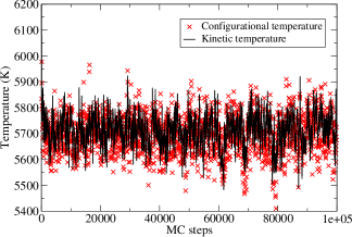
Figure 1: Comparison between configurational and kinetic instantaneous temperatures during a MC simulation for $N$=864 atoms.

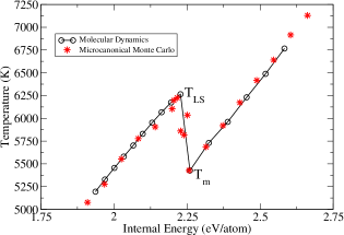
Figure 2: Comparison between the isochoric curves obtained by standard, microcanonical molecular dynamics and microcanonical MC methods, for a system of $N$=864 atoms.

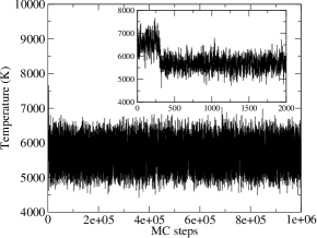
Figure 3: Evolution of the instantaneous temperature during a MC simulation where melting is observed, for $N$=108 atoms. Total simulation comprises 1 million MC steps, and the inset shows the first 2000 MC steps.

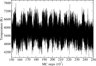
Figure 4: Alternation between solid and liquid phases as seen from the instantaneous temperature, for a MC simulation with $N$=72 atoms.

IV Summary and conclusions

Belonoshko et al Belonoshko et al. (2007) attributed the success of the Z method in reaching the highest $T_{LS}$ among several molecular dynamics methods to the preservation of the natural dynamics of the system. However, we have shown this is not the case: using a MC algorithm which is completely oblivious to the equations of motion we have reproduced the same $T_{LS}$ and the same $T_{m}$ as in standard molecular dynamics. This suggests that the previously thought advantage of the Z method comes from a different direction, namely, that the preservation of the microcanonical condition is the important fact, and the specific trajectory followed by each atom is not important. Therefore, any method capable of computing microcanonical averages should be just as reliable in Z method computations.

Practical consequences of this finding are clear in terms of the efficiency for large or complex systems. The success of MC methods in the determination of the Z curve hints to the possibility of a fully-parallelizable version of the method.

V Acknowledgements

SD acknowledges financial support from FONDECYT grant 1140514. GG and SD thank partial support from CONICYT-PIA grant ACT-1115, Chile.

References

- Alfè et al. (2004) D. Alfè, L. Vočadlo, G. D. Price, and M. J. Gillan, J.Phys.: Condens. Matter 16, S973 (2004).
- Belonoshko et al. (2000) A. B. Belonoshko, R. Ahuja, and B. Johansson, Phys. Rev. Lett. 84, 3638 (2000).
- Oganov et al. (2005) A. R. Oganov, G. D. Price, and S. Scandolo, Z. Krist. 220, 531 (2005).
- Cavazzoni et al. (1999) C. Cavazzoni, G. L. Chiarotti, S. Scandolo, E. Tosatti, M. Bernasconi, and M. Parrinello, Science 283, 44 (1999).
- Padture et al. (2002) N. P. Padture, M. Gell, and E. H. Jordan, Science 296, 280 (2002).
- Datchi et al. (2000) F. Datchi, P. Loubeyre, and R. LeToullec, Phys. Rev. B 61, 6535 (2000).
- Tallon (1989) J. L. Tallon, Nature 342, 658 (1989).
- Jin et al. (2001) Z. H. Jin, P. Gumbsch, K. Lu, and E. Ma, Phys. Rev. Lett. 87, 055703 (2001).
- Forsblom and Grimvall (2005) M. Forsblom and G. Grimvall, Nature Materials 4, 388 (2005).
- Belonoshko (1994) A. B. Belonoshko, Geochim. Cosmochim. Acta 58, 4039 (1994).
- Morris et al. (1994) J. R. Morris, C. Z. Wang, K. M. Ho, and C. T. Chan, Phys. Rev. B 49 (1994).
- Sugino and Car (1995) O. Sugino and R. Car, Phys. Rev. Lett. 74, 1823 (1995).
- de Wijs et al. (1998) G. A. de Wijs, G. Kresse, and M. J. Gillian, Phys. Rev. B 57, 8223 (1998).
- de Koning et al. (1999) M. de Koning, A. Antonelli, and S. Yip, Phys. Rev. Lett. 83, 3973 (1999).
- Donadio et al. (2010) D. Donadio, L. Spanu, I. Duchemin, F. Gygi, and G. Galli, Phys. Rev. B 82, 020102 (2010).
- Gulminelli and Chomaz (2002) F. Gulminelli and P. Chomaz, Phys. Rev. E 66, 046108 (2002).
- Campa et al. (2009) A. Campa, T. Dauxois, and S. Ruffo, Phys. Rep. 480, 57 (2009).
- Pearson et al. (1985) E. M. Pearson, T. Halicioglu, and W. A. Tiller, Phys. Rev. A 32, 3030 (1985).
- Lustig (1998) R. Lustig, J. Chem. Phys. 109, 8816 (1998).
- Gross and Votyakov (2000) D. H. E. Gross and E. Votyakov, Eur. Phys. J. B 15, 115 (2000).
- Gross (2005) D. H. E. Gross, Physica E 29, 251 (2005).
- Westergren et al. (2003) J. Westergren, S. Nordholm, and A. Rosén, Phys. Chem. Chem. Phys. 5, 136 (2003).
- Junghans et al. (2006) C. Junghans, M. Bachmann, and W. Janke, Phys. Rev. Lett. 97, 218103 (2006).
- Hernández-Rojas and Gomez Llorente (2008) J. Hernández-Rojas and J. M. Gomez Llorente, Phys. Rev. Lett. 100, 258104 (2008).
- Bereau et al. (2011) T. Bereau, M. Deserno, and M. Bachmann, Biophysical Journal 100, 2764 (2011).
- Belonoshko et al. (2006) A. B. Belonoshko, N. V. Skorodumova, A. Rosengren, and B. Johansson, Phys. Rev. B 73, 012201 (2006).
- Davis et al. (2011) S. Davis, A. B. Belonoshko, B. Johansson, and A. Rosengren, Phys. Rev. B 84, 064102 (2011).
- Severin et al. (1978) E. S. Severin, B. C. Freasier, N. D. Hamer, D. L. Jolly, and S. Nordholm, Chem. Phys. Lett. 57, 117 (1978).
- Ray (1991) J. R. Ray, Phys. Rev. A 44, 4061 (1991).
- Creutz (1983) M. Creutz, Phys. Rev. Lett. 50, 1411 (1983).
- Rugh (1997) H. H. Rugh, Phys. Rev. Lett. 78, 772 (1997).
- Butler et al. (1998) B. D. Butler, G. Ayton, O. G. Jepps, and D. J. Evans, J. Chem. Phys. 109, 6519 (1998).
- Rickayzen and Powles (2001) G. Rickayzen and J. G. Powles, J. Chem. Phys. 114, 4333 (2001).
- Alfè et al. (2011) D. Alfè, C. Cazorla, and M. J. Gillan (2011), eprint arXiv:1104.2147v1.
- Evans and Searles (2002) D. J. Evans and D. J. Searles, Advances in Physics 51, 1529 (2002).
- Swendsen and Wang (1987) R. H. Swendsen and J. S. Wang, Phys. Rev. Lett. 58, 86 (1987).
- Wolff (1989) U. Wolff, Phys. Rev. Lett. 62, 361 (1989).
- Binder and Heermann (2010) K. Binder and D. W. Heermann, Monte Carlo Simulation in Statistical Physics: An Introduction (Springer, 2010).
- Belonoshko et al. (2007) A. B. Belonoshko, S. Davis, N. V. Skorodumova, P. H. Lundow, A. Rosengren, and B. Johansson, Phys. Rev. B 76, 064121 (2007).