Stochastic Flow Models with Delays and Applications to Multi-Intersection Traffic Light Control

Abstract

We extend Stochastic Flow Models (SFMs), used for a large class of discrete event and hybrid systems, by including the delays which typically arise in flow movement. We apply this framework to the multi-intersection traffic light control problem by including transit delays for vehicles moving from one intersection to the next. Using Infinitesimal Perturbation Analysis (IPA) for this SFM with delays, we derive new on-line gradient estimates of several congestion cost metrics with respect to the controllable green and red cycle lengths. The IPA estimators are used to iteratively adjust light cycle lengths to improve performance and, in conjunction with a standard gradient-based algorithm, to obtain optimal values which adapt to changing traffic conditions. We introduce two new cost metrics to better capture congestion and show that the inclusion of delays in our analysis leads to improved performance relative to models that ignore delays.

1 INTRODUCTION

Stochastic Flow Models (SFMs) capture the dynamic behavior of a large class of hybrid systems (see Cassandras and Lafortune (2009)). In addition, they are used as abstractions of Discrete Event Systems (DES), for example when discrete entities accessing resources are treated as flows. The basic building block in a SFM is a queue (buffer) whose fluid content is dependent on incoming and outgoing flows which may be controllable. By connecting such building blocks together, one can generate stochastic flow networks which are encountered in application areas such as manufacturing systems (Armony et al. (2015)), chemical processes (Yin et al. (2013)), water resources (Anderson et al. (2015)), communication networks (Cassandras et al. (2002)) and transportation systems (Geng and Cassandras (2015)). Figure 1 shows a two-node SFM, in which an on-off switch controls the outgoing flow for each node. When the switch at the output of node $1$ is turned on, a “flow burst” is generated to join the downstream node $2$. Flow models commonly assume that this flow burst can instantaneously join the downstream queue, thus ignoring potentially significant delays before this can happen. Incorporating such delays through more accurate modeling is challenging but crucial in better evaluating the performance of the underlying system and seeking ways to improve it.

Control mechanisms used in SFMs often involve gradient-based methods in which the controller uses estimates of the performance metric sensitivities with respect to controllable parameters in order to adjust the values of these parameters and improve (ideally, optimize) performance. Infinitesimal Perturbation Analysis (IPA) is a method of general applicability to stochastic hybrid systems (see Cassandras et al. (2010),Wardi et al. (2010)) through which gradients of performance measures may be estimated with respect to several controllable parameters based on directly observable data. The applications of IPA and its advantages have been reported elsewhere (e.g., Cassandras et al. (2010),Fleck et al. (2016)) and are summarized here as follows: $(i)$ IPA estimates have been shown to be unbiased under very mild conditions (Cassandras et al. (2010)). $(ii)$ IPA estimators are robust with respect to the stochastic processes involved. $(iii)$ IPA is event-driven, hence scalable in the number of events in the system, not the (much larger) state space dimensionality. $(iv)$ IPA possesses a decomposability property (Yao and Cassandras (2011)), i.e., IPA state derivatives become memoryless after certain events take place. $(v)$ The IPA methodology can be easily implemented on line, allowing us to take advantage of directly observed data.

While IPA has been extensively used in SFMs, the effect of delays between adjacent nodes, as described above, has not been studied to date. Thus, the contribution of this paper is to incorporate delays in the flow bursts that are created by on-off switching control (see Fig. 1) into the standard SFM and to develop the necessary extensions to IPA for such systems. In addition, an application of SFMs with delays to the Traffic Light Control (TLC) problem in transportation networks is included.

The rest of the paper is organized as follows. In Section 2, we extend the standard multi-node SFM to include delays. In Section 3 we adapt this model to the TLC problem by explicitly modeling the delay experienced by vehicles moving from one intersection to the next. This allows us to introduce two new cost metrics for congestion that incorporate the effect of delays. In Section 4, we carry out IPA for the TLC problem and in Section 5 we provide simulation examples comparing performance results between a model considering traffic delays and one which does not, showing that the former achieves improved performance.

2 STOCHASTIC FLOW MODELS WITH DELAYS

Consider a two-node SFM as in Fig. 1 and let $\{\alpha_{i}(t)\}$ and $\{\beta_{i}(t)\}$, $i=1,2$, be the incoming flow and outgoing flow processes respectively. We emphasize that these are both treated as random processes. We define $x(t)=[x_{1}(t),x_{2}(t)]$, where $x_{i}(t)\in\mathbb{R}^{+}$ is the flow content of node $i$ (we assume that all variables are left-continuous.) The dynamics of this SFM are

$$\dot{x}_{i}(t)=\left\{\vspace*{0pt}\begin{array}[c]{l}0\\ \\ \alpha_{i}(t)-\beta_{i}(t)\end{array}\right.\begin{array}[c]{l}\text{if }x_{i}(t)=0,\text{ }\alpha_{i}(t)\leq\beta_{i}(t)\\ \text{or }x_{i}(t)=c_{i},\text{ }\alpha_{i}(t)\geq\beta_{i}(t)\\ \text{otherwise}\end{array}$$ (1)

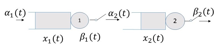
Figure 1: A two-node SFM.

where $c_{i}$ is the content capacity of $i$ and $\beta_{i}(t)$ is

$$\vspace*{-1pt}\beta_{i}(t)=\left\{\begin{array}[c]{l}h_{i}(t)\\ 0\end{array}\right.\begin{array}[c]{l}\text{if }G_{i}(t)=1\\ \text{otherwise}\end{array}$$ (2)

in which $h_{i}(t)$ is the instantaneous outgoing flow rate at node $i$, and $G_{i}(t)\in\{0,1\}$, $i=1,2$ is a switching controller. We also define a clock state variable $z_{i}(t)$ for each switching controller $G_{i}(t)$:

$$\dot{z}_{i}(t) =\left\{\begin{array}[c]{l}1\\ 0\end{array}\right.\begin{array}[c]{l}\text{if }G_{i}(t)=1\\ \text{otherwise}\end{array}$$ (7)

$$z_{i}(t^{+}) =0\text{ \ \ if }G_{i}(t)=1\text{ and }G_{i}(t^{+})=0$$

Thus, when $G_{1}(t)=1,$ $t\in[t_{1},t_{2})$, $G_{1}(t_{1}^{-})=0$, a flow burst is created at node $1$ (when $x_{1}(t_{1})>0$). In general, several such flow bursts may be created over $(t_{1},t_{2}]$, depending on the values of $\alpha_{1}(t)$, $h_{1}(t),$ $t\in(t_{1},t_{2}]$. In SFMs studied to date, we ignore the delay incurred by any such flow burst being transferred between nodes and assume that it instantaneously joins the queue at node $2$. Under this assumption,

$$\vspace*{-1pt}\alpha_{2}(t)=\left\{\begin{array}[c]{l}\alpha_{1}(t)\\ \beta_{1}(t)\end{array}\right.\begin{array}[c]{l}\text{if }x_{1}(t)=0,\text{ }\alpha_{1}(t)\leq\beta_{1}(t)\\ \text{otherwise}\end{array}$$

In what follows, we extend the SFM to include the aforementioned delay which depends on when a flow burst actually joins the downstream queue, an event that we need to carefully specify. While a flow burst is in transit between nodes $1$ and $2$, let $x_{12}(t)$ be its size, i.e.,the flow volume in transit before it joins $x_{2}(t)$. For simplicity, we assume that each flow burst is maintained during this process (i.e., the burst may not be separated in two or more sub-bursts). We will use $L$ to denote the physical distance between nodes 1 and 2.

Predicting the time when the first flow burst actually joins queue $2$ is complicated by the fact that $x_{2}(t)$ evolves while this burst is in transit. This is illustrated through the example in Fig. 2 which we will use to describe the evaluation of this time through a sequence of events denoted by $\{J_{1},\ldots,J_{K}\}$ with associated event times $\{\sigma_{1},\ldots,\sigma_{K}\}$. We define $J_{0}$ to be the event when the flow burst leaves node $1$, i.e., the occurrence of a switch from $G_{1}(t^{-})=0$ to $G_{i}(t)=1$, and let $\sigma_{0}$ be its associated occurrence time. Therefore, an estimate of the time when the flow burst joins the tail of queue $2$ is given by $\sigma_{1}=\sigma_{0}+[L-x_{2}(\sigma_{0})]/v(\sigma_{0})$ where $v(\sigma_{0})$ is the “speed” of the flow burst which we assume to be constant and, for notational simplicity, set it to $v(\sigma_{0})=1$ (it will become clear in the sequel that this can be relaxed and treated as random in the context of IPA). Thus, we define $J_{1}$ to be the event at time $\sigma_{1}$ when the flow burst covers the distance $L-x_{2}(\sigma_{0})$. In general, however, $x_{2}(\sigma_{1})\leq{x}_{2}(\sigma_{0})\equiv\bar{x}_{2}(\sigma_{1})$, i.e., the estimate $\bar{x}_{2}(\sigma_{1})$ of $x_{2}(\sigma_{1})$ is based on the assumption that $x_{2}(t)$ remains unchanged over $(\sigma_{0},\sigma_{1})$. This is illustrated in the example of Fig. 2, where $\dot{x}_{2}(t)=-\beta_{2}(t)<0$ for some $t\in(\sigma_{0},\sigma_{1})$. Thus, unless $x_{2}(\sigma_{1})={x}_{2}(\sigma_{0})$, we repeat at $t=\sigma_{1}$ the same process of estimating the time of the next opportunity that the flow burst might join queue $2$ at time $\sigma_{2}$ to cover the distance $\bar{x}_{2}(\sigma_{1})-x_{2}(\sigma_{1})$ and define this potential joining event as $J_{2}$. 2. This process continues until event $J_{K}$ occurs at time $\sigma_{K}$, the last event in the sequence $\{J_{1},\ldots,J_{K}\}$ when $\bar{x}_{2}(\sigma_{K})=x_{2}(\sigma_{K})$. Note that $J_{K}$ may occur either when $(i)$ $\bar{x}_{2}(\sigma_{K})=x_{2}(\sigma_{K})>0$, in which case the estimate $\bar{x}_{2}(\sigma_{K})$ incurs no error because $x_{2}(\sigma_{K})=x_{2}(\sigma_{K-1})$, i.e., the queue length at node $2$ remained unchanged because $\beta_{2}(t)=0$ for $t\in[\sigma_{K-1},\sigma_{K}]$, or $(ii)$ $\bar{x}_{2}(\sigma_{K})=x_{2}(\sigma_{K})=0$, in which case the flow burst joins node $2$ while this queue is empty. Since in practice the queues and flow bursts may consist of discrete entities (e.g., vehicles), we define event $J_{K}$ as occurring when $\bar{x}_{2}(t)-x_{2}(t)\leq\epsilon$ for some predefined fixed small $\epsilon$, i.e., a flow burst joins the downstream queue whenever it is sufficiently close to it. The following lemma asserts that the event time sequence $\{\sigma_{1},\ldots,\sigma_{K}\}$ is finite.

Lemma 1. Under the assumption that $J_{K}$ is defined through $\bar{x}_{2}(\sigma_{K})-x_{2}(\sigma_{K})\leq\epsilon$, the number of events $K$ in $\{J_{1},\ldots,J_{K}\}$ is bounded. Moreover, its event time $\sigma_{K}$ is also bounded.

Proof: Observe that $x_{2}(t)\leq L$, since the content of queue $2$ is limited by the physical distance $L$. In addition, $\bar{x}_{2}(t)-x_{2}(t)>\epsilon$ prior to event $J_{K}$. It follows that $K\leq L/\epsilon$. Moreover, in the worst case, a flow burst travels the finite distance $L$ to find $x_{2}(\sigma_{K})=0$, therefore, $\sigma_{K}\leq\sigma_{0}+L-x_{2}(\sigma_{0})$. $\blacksquare$

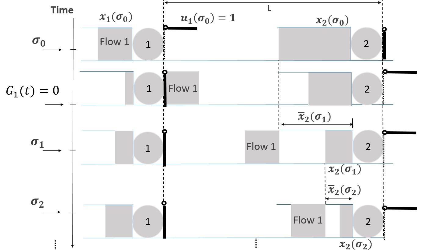
Figure 2: Typical evolution of a flow burst in transit.

We now formalize the dynamics of the flow transit process described above. First, the dynamics of $\bar{x}_{2}(t)$, the estimated queue length when an event $J_{k}$ occurs, are given by

$$\dot{\bar{x}}_{2}(t) =0$$ (8)

$$\bar{x}_{2}(t^{+}) =x_{2}(t)\text{ \ if }t=\sigma_{k},\text{ }k=1,...,K.\vspace{0pt}$$

with $\bar{x}_{2}(\sigma_{1})=L-x_{2}(\sigma_{0})$ and $\sigma_{0}$ defined above as the occurrence time of a switch from $G_{1}(t^{-})=0$ to $G_{i}(t)=1$. The dynamics of $x_{12}(t)$ are given by

$$\dot{x}_{12}(t) =\left\{\begin{array}[c]{l}0\\ \alpha_{1}(t)\\ h_{1}(t)\end{array}\right.\begin{array}[c]{l}\text{if }G_{1}(t)=0\\ \text{if }x_{1}(t)=0,\text{ }\alpha_{1}(t)\leq\beta_{1}(t)\\ \text{otherwise}\end{array}$$ (15)

$$x_{12}(t^{+}) =0\text{ \ \ if }t=\sigma_{K}$$

The dynamics of $x_{2}(t)$ are no longer described by (1), since the queue content is only updated when a flow burst joins queue 2 at time $\sigma_{K}$. Instead, they are given by

$$\dot{x}_{2}(t) =\left\{\vspace*{0pt}\begin{array}[c]{l}-\beta_{i}(t)\\ 0\end{array}\right.\begin{array}[c]{l}\text{if }x_{2}(t)>0\text{ and }G_{2}(t)=1\\ \text{otherwise}\end{array}$$ (20)

$$x_{2}(\sigma_{K}^{+}) =x_{2}(\sigma_{K})+x_{12}(\sigma_{K})$$

Note that in (8) and (15) the values of event times $\{\sigma_{1},\ldots,\sigma_{K}\}$ remain unspecified. In order to provide this specification, we define $\delta_{12}(t)=\bar{x}_{2}(t)-x_{2}(t)$ to be the distance between the head of the flow burst and the tail of $x_{2}(t)$. Then, observe that $\sigma_{k}=\sigma_{k-1}+\tau(\delta_{12}(\sigma_{k-1}))$, where $\tau(r)$ is the time to complete a distance $r\in(0,L]$ and $k=1,...,K-1$. Similar to the clock $z_{i}(t)$ in (7) that dictates the timing of the controlled switching process, we associate a clock $z_{12}(t)$ to the timing of events in $\{J_{1},\ldots,J_{K}\}$ as follows:

$$\dot{z}_{12}(t) =\left\{\begin{array}[c]{l}1\\ 0\end{array}\right.\begin{array}[c]{l}\text{if }{\delta_{12}(t)>0}\\ \text{otherwise}\end{array}$$ (25)

$$z_{12}(t^{+}) =0\text{ \ \ if }z_{12}(t)=\tau({\delta_{12}(t)})$$

with an initial condition $z_{12}(\sigma_{0})=0$ and

$$\dot{\delta}_{12}(t) =0$$ (26)

$$\delta_{12}(t^{+}) =\left\{\begin{array}[c]{l}L-x_{2}(t)\\ \bar{x}_{2}(t)-x_{2}(t)\end{array}\right.\begin{array}[c]{l}\text{if }t=\sigma_{0}\\ \text{if }t=\sigma_{k},k=1,...,K.\end{array}\vspace*{0pt}$$ (31)

Note that $\delta_{12}(t)$ is piecewise constant and updated only at the times when events $J_{0},J_{1},\ldots,J_{K}$ take place ending with $\delta_{12}(t^{+})=0$ when event $J_{K}$ occurs, i.e., the flow burst joins queue $2$. The values of $\tau({\delta_{12}(t)})$ in (25) are given by the time required for the flow burst to travel a distance ${\delta_{12}(t)=}\bar{x}_{2}(t)-x_{2}(t)$ with speed $v(\sigma_{0})$ which we assumed earlier to be constant and set to $v(\sigma_{0})=1$. Thus, $\tau(\delta_{12}(t))=\delta_{12}(t)$. Finally, note that in this modeling framework, we assume that $x_{2}(t)$ is observable at event times $\sigma_{0},\sigma_{1},\ldots,\sigma_{K}$ when events $J_{0},J_{1},\ldots,J_{K}$ take place.

As a final step, we generalize this model to include multiple flow bursts that may be generated in an interval $(t_{1},t_{2}]$ such that $G_{1}(t)=1$ for $t\in[t_{1},t_{2})$, $G_{1}(t_{1}^{-})=0$. Thus, we denote by $J_{k}^{n}$ the $k$th event for the $n$th flow burst to (potentially) join queue $2$ and extend $\delta_{12}(t)$ to $\delta_{12}^{n}(t)$, $\sigma_{k}$ to $\sigma_{k}^{n}$, and $x_{12}(t)$ to $x_{12}^{n}(t)$, $n=1,2,\ldots$ Also, we define $J_{i,j}$ as an event such that the $i$th flow burst merges with the $j$th burst at time $\tau_{i,j}$. For simplicity, we use $y^{m}(t)$ to represent $x_{12}^{m}(t)$. We then have:

$$\dot{x}_{12}^{n}(t) =\left\{\begin{array}[c]{l}\alpha_{1}(t)\\ h_{1}(t)\\ \\ 0\\ \end{array}\right.\begin{array}[c]{l}\text{if }n=1,x_{1}(t)=0,\text{ }\alpha_{1}(t)<\beta_{1}(t)\\ \text{if }n=1,G_{1}(t)=1\\ x_{1}(t)=0,\text{ }\alpha_{1}(t)\geq\beta_{1}(t)\text{ or }x_{1}(t)>0\\ \text{otherwise}\end{array}$$ (40)

$$x_{12}^{n}(t^{+}) =0\text{ \ \ if }t=\sigma_{K}^{n}\text{ or }t=\tau_{n,n-1}$$ (41)

$$x_{12}^{n}(t^{+}) =x_{12}^{n}(t)+x_{12}^{n-1}(t)\text{ \ \ if }t=\tau_{n+1,n}$$

$$\dot{\delta}_{12}^{n}(t) =0$$ (42)

$$\delta_{12}^{n}(t^{+}) =\left\{\begin{array}[c]{l}L-x_{2}(t)\\ \bar{x}_{2}^{n}(t)-x_{2}(t)\\ \delta_{12}^{n}(t)-y^{m}(t)\end{array}\right.\begin{array}[c]{l}\text{if }t=\sigma_{0}^{n}\\ \text{if }t=\sigma_{k}^{n},k>0\\ \text{if }t=\sigma_{K}^{m},m=1,\ldots,n-1\end{array}$$ (49)

$$\dot{\bar{x}}_{2}^{n}(t) =0$$ (50)

$$\bar{x}_{2}^{n}(t^{+}) =\left\{\begin{array}[c]{l}x_{2}(t)\\ x_{2}(t)+y^{m}(t)\end{array}\right.\begin{array}[c]{l}\text{if }t=\sigma_{k}^{n},k\geq 0\\ \text{if }t=\sigma_{K}^{m},m=1,\ldots,n-1\end{array}$$ (55)

with the obvious generalizations of (8)-(26).

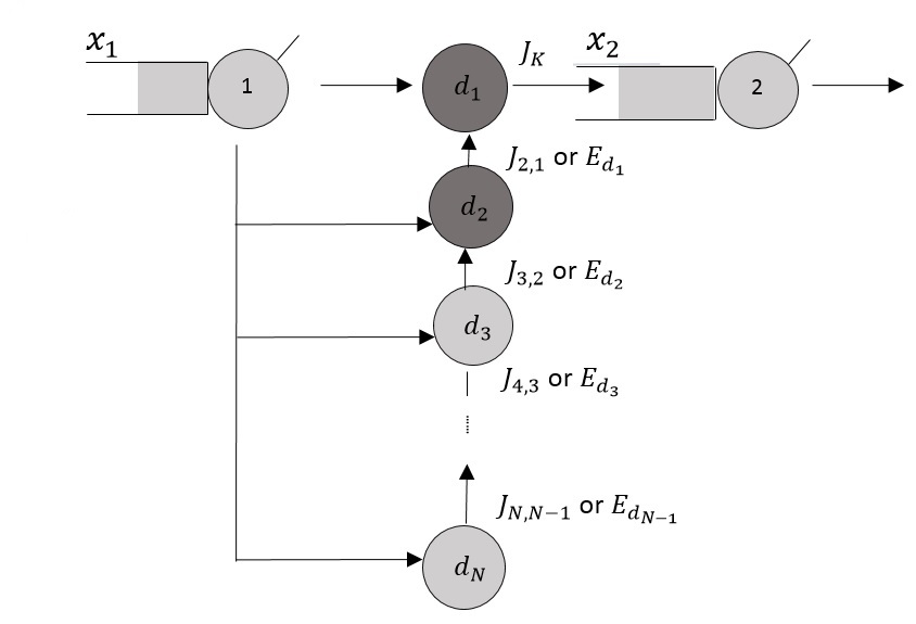
Figure 3: Two-node SFM with delay.

The generalized SFM with delay is shown in Fig. 3. We define a series of servers $d_{n}$, $n\in\{j\in\mathbb{Z}:j=1,\ldots,N\}$ to describe the flow transit delay between SFM where $y_{n}(t)$ is the content of $d_{n}$. Here, $N$ is the total number of servers required depending on a specific application. For example, in the two-intersection traffic system discussed in the next section, we set $N=\lceil L/L_{v}\rceil$ where $L$ is the physical distance between intersections and $L_{v}$ is the length of a vehicle. When a new flow burst leaves server $1$, the controlled switching process checks whether $y_{1}(t)=0$ to initiate a flow burst. If $y_{1}(t)>0$, it checks $y_{j}(t)$ for $j\geq 2$ until some $y_{j}(t)=0$. For example, in Fig. 3, if servers $d_{1}$ and $d_{2}$ are non-empty (dark color), and $d_{3}$ is empty (light color), the new flow burst will join server $d_{3}$ until $y_{1}(t)=0$. The first flow burst will leave server $d_{1}$ when event $J_{K}^{1}$ occurs and joins $x_{2}(t)$. The flow burst in server $d_{n}$ will leave when either one of two events occurs, defined as follows: (1) $J_{n,n-1}$ occurs when the $n$th flow burst joins the $(n-1)$th burst. (2) $E_{d_{n-1}}$ occurs when $y_{n-1}(t)=0$.

SFM Events. The hybrid system with dynamics given by (1)-(26) defines the SFM with transit delays. To complete the model, we define next the event set associated with all discontinuous state transitions in (1)-(26). As in prior work using SFMs, we observe that the sample path of any queue content process in our model can be partitioned into Non-Empty Periods (NEPs) when $x_{i}(t)>0$, and Empty Periods (EPs) when $x_{i}(t)=0$. Let us define the start of a NEP at queue $i$ as event $S_{i}$ ($S_{12}$ for queue $12$) and the end of a NEP at queue $i$ as event $E_{i}$ ($E_{12}$ for queue $12$). In (1), observe that $S_{1}$ is an event that can be induced by either an event such that $\alpha_{1}(t)-\beta_{2}(t)$ switches from $\leq 0$ to $>0$ or by an event which switches the value of $\beta_{1}(t)$; moreover, in (2), the value of $\beta_{1}(t)$ switches when an event occurs such that $G_{1}(t)$ changes between $0$ and $1$. In (20), $S_{2}$ may also be induced by event $J_{k}$ if it occurs when $x_{2}(t)=0$. Finally, in (15), $S_{12}$ is induced by the same events that induce $S_{2}$, while $E_{12}$ is induced by $J_{K}$ since that causes the end of the flow burst that created $x_{12}(t)>0$. To sum up, there are five events that can affect any of the processes $\{x_{1}(t)\}$, $\{x_{2}(t)\}$ and $\{x_{12}(t)\}$:

1. $E_{i}$: $x_{i}(t)$ switches from $>0$ to $=0$, thus ending a NEP at queue $i$.

2. $\Gamma_{i}$: $\alpha_{i}(t)-\beta_{i}(t)$ switches from $\leq 0$ to $>0$.

3. $J_{k}$: $z_{12}(t)=\tau({\delta_{12}(t)})$ representing a potential joining of the flow burst $x_{12}(t)$ with $x_{2}(t)$ if ${\delta_{12}(t^{+})>0}$, or the actual joining if ${\delta_{12}(t^{+})=0}$.

4. $C2O_{i}$: $G_{i}(t)$ switches from $1$ to $0$.

5. $O2C_{i}$: $G_{i}(t)$ switches from $0$ to $1$.

We can now identify the event set that affects the dynamics of the three queue content processes:

$$\Phi_{1} =\{S_{i},E_{i},O2C_{i},C2O_{i}\}\text{,}$$

$$\Phi_{2} =\{S_{2},E_{2},O2C_{2},C2O_{2},J_{k}\},\text{ }\Phi_{12}=\{S_{12},E_{12},E_{1},C2O_{1},J_{k}\}$$

Finally, note that this SFM model can be extended to any network of queues with possible delays by identifying queues with dynamics of type (1) or (20) or (15).

3 MULTI-INTERSECTION TRAFFIC LIGHT CONTROL WITH DELAYS

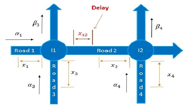
Figure 4: Two traffic intersections.

An application of the SFM with delays arises in the Traffic Light Control (TLC) problem in transportation networks, which consists of adjusting green and red signal settings in order to control the traffic flow through an intersection and, more generally, through a set of intersections and traffic lights in an urban roadway network. The ultimate objective is to minimize congestion in an area consisting of multiple intersections. Many methods have been proposed to solve the TLC problem, including expert systems, genetic algorithms, reinforcement learning and several optimization techniques; a more detailed review of such methods may be found in Fleck et al. (2016). Perturbation analysis methods were used in Head et al. (1996) and Fu and Howell (2003). IPA was used in Panayiotou et al. (2005) and Geng and Cassandras (2012) for a single intersection and extended to multiple intersections in Geng and Cassandras (2015) and to quasi-dynamic control schemes in Fleck et al. (2016). However, all this work to date has assumed that vehicles moving from one intersection to the next experience no delay. In this section, we formulate the TLC problem by including delays as in Section 2 and derive an IPA-based controller to optimize selected performance metrics (cost functions). By including delays, we will see that we can define new metrics which capture “congestion” in traffic systems much more accurately.

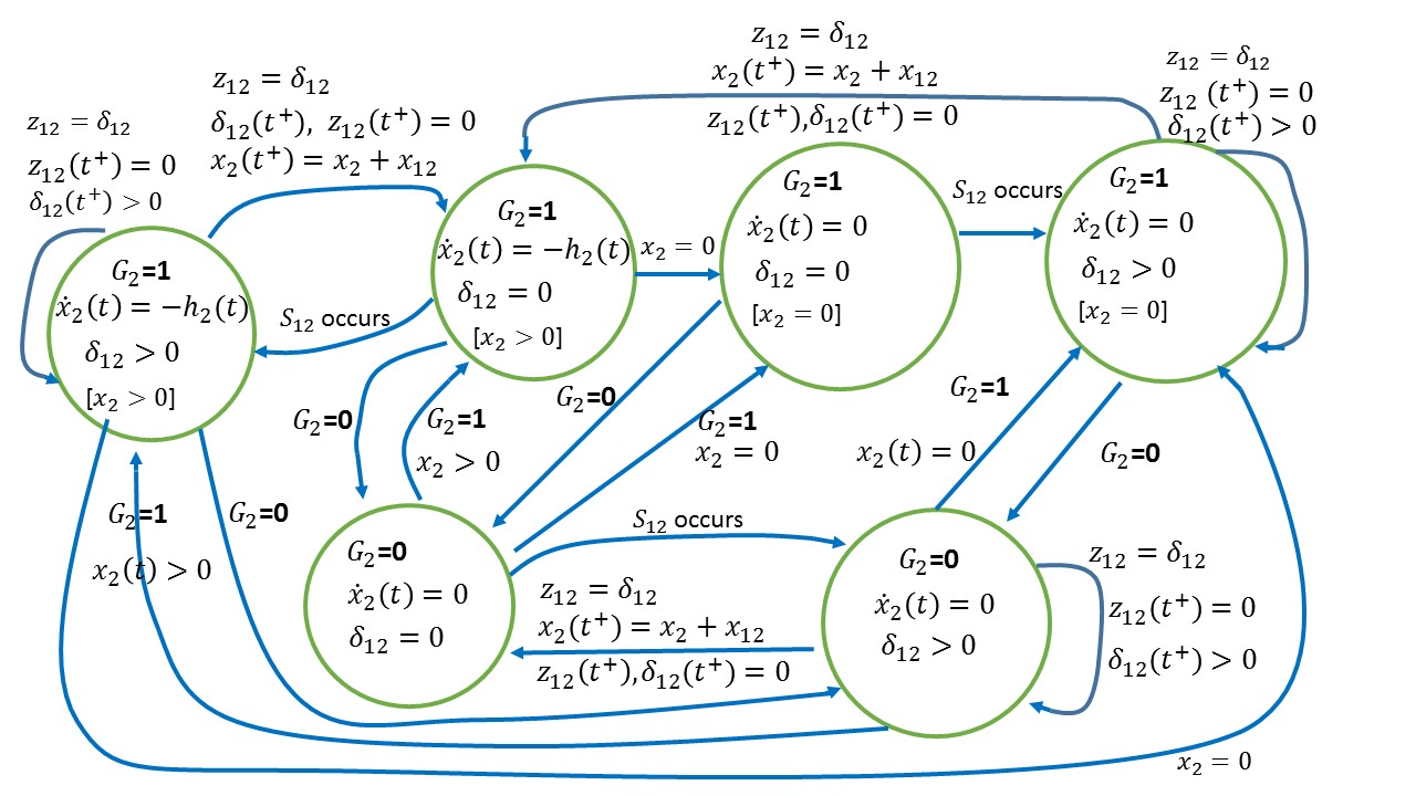
Figure 5: Stochastic Hybrid Automaton model for $x_{2}(t)$.

As in Section 2, let $\{\alpha_{i}(t)\}$ and $\{\beta_{i}(t)\}$, $i=1,\ldots,4$, be the incoming and outgoing flow processes respectively at all four roads shown in Fig. 4, where we now interpret $\alpha_{i}(t)$ as the random instantaneous vehicle arrival rate at time $t$. We define the controllable parameters $\theta_{i}$ to be the durations of the GREEN light for road $i=1,\ldots,4$. Thus, the state vector is $x(\theta,t)=[x_{1}(\theta,t),x_{2}(\theta,t),x_{3}(\theta,t),x_{4}(\theta,t),x_{12}(\theta,t)]$ where $x_{i}(\theta,t)$ is the content of queue $i$ and $x_{12}(\theta,t)$ is the content of the road between intersections $I1$ and $I2$. To maintain notational simplicity, we will assume in our analysis that (A1) There is no more than one traffic burst in queue $12$ at any one time, (A2) The speed of a traffic burst $v_{1}(t)$ between intersections is constant, and (A3) There is no traffic coupling between $I1$ and $I2$. Assumptions (A1) and (A2) simplify the analysis and can be easily relaxed since our model can deal with multiple flow bursts as shown in Section 2. Assumption (A3) means that the distance between $I2$ and $I1$ is sufficiently large and is also made to simplify the model; it can be relaxed along the lines of Geng and Cassandras (2015).

We define clock state variables $z_{i}(t)$, $i=1,\ldots,4$, which are associated with the GREEN light cycle for queue $i$ based on (7) where the controller $G_{i}(t)$ is now the traffic light state, i.e., $G_{i}(t)=0$ means that the traffic light in road $i$ is RED, otherwise, it is GREEN. Accordingly, the departure rates and the queue content dynamics $x_{i}(t)$, $i=1,\ldots,4$, are given by (1)-(20).

In order to provide the dynamics of $x_{2}(t)$ and $x_{12}(t)$, we will make use of our analysis in Section 2. In particular, let $\sigma_{0}$ be the time when a positive traffic flow is generated from queue $1$ and enters queue $12$, i.e., the light turns from RED to GREEN for road $1$ and $x_{1}(\sigma_{0})>0$. Invoking (26), we define $\delta_{12}(t)$ to be the distance between the head of the “transit queue” $12$ and the tail of queue $2$. Thus, $\delta_{12}(\sigma_{0}^{+})=L-x_{2}(\sigma_{0})$. We also associate a clock to this queue, denoted by $z_{12}(t)$, which is defined by (25) and initialized at $z_{12}(\sigma_{0})=0$. Finally, $\tau(\delta_{12}(t))$ in (25) in the TLC context is given by $\tau(\delta_{12}(t))=\delta_{12}(t)/v_{1}$.

Recall that a $J_{k}$ event represents a potential joining of the flow burst from $I1$ with queue $2$. The actual joining event occurs when ${\delta_{12}(t^{+})=0}$ from its initial value $\delta_{12}(\sigma_{0}^{+})=L-x_{2}(\sigma_{0})$. Adapting (26) and (8) to the TLC setting we get the dynamics of $\delta_{12}$ and $\bar{x}_{2}(t)$, while the dynamics of $x_{2}(t)$ and $x_{12}(t)$ are given by (20) and (15) respectively.

SFM Events. We apply the event set defined in Section 2 where we use $G2R_{i}$ (traffic light $i$ changes from GREEN to RED) to replace $C2O_{i}$ and $R2G_{i}$ to replace $O2C_{i}$. Figure 5 shows the hybrid automaton model for queue 2 in terms of its six possible modes depending on $x_{2}(t)$, $G_{2}(t)$ and $\delta_{12}(t)$. Similar models apply to the remaining processes, all of which are generally interdependent(e.g., in Fig.5, some reset conditions involve $x_{12}(t)$).

Cost Functions. The objective of the TLC problem is to control the green cycle parameters $\theta_{i}$, $i=1,\ldots,4$, so as to minimize traffic congestion in the region covered by the two intersections in Fig. 4. In Geng and Cassandras (2012) and Fleck et al. (2016), the average total weighted queue lengths over a fixed time interval $[0,T]$ is used to capture congestion:

$$F(\theta;x(0),z(0),T)=\frac{1}{T}\sum_{i=1}^{5}\int_{0}^{T}w_{i}x_{i}(\theta,t)dt.$$ (56)

where $w_{i}$ is the weight associated with queue $i$. For convenience, we will refer to (56) as the average queue cost function; with a slight abuse of notation we have re-indexed $x_{12}(t)$ as $x_{5}(t)$. However, this may not be an adequate measure of “congestion”. For instance, it is possible that the average queue lengths over $[0,T]$ are relatively small, while reaching large values over small intervals (peak periods during a typical day). Thus, instead of restricting ourselves to (56), we define next two new cost functions.

1. Average weighted $P$th power of the queue lengths over a fixed interval $[0,T)$, where $P>1$. The sample function is

$$F(\theta;x(0),z(0),T)=\frac{1}{T}\sum_{i=1}^{5}\int_{0}^{T}w_{i}x_{i}^{P}(\theta,t)dt.$$

Observing that $x_{i}(\theta,t)=0$ during an EP of queue $i$, we can rewrite this as

$$F(\theta;x(0),z(0),T)=\frac{1}{T}\sum_{i=1}^{5}\sum_{m=1}^{M_{i}}\int_{\xi_{i,m}}^{\eta_{i,m}}w_{i}x_{i}^{P}(\theta,t)dt,$$ (57)

in which $M_{i}$ is the total number of NEPs of queue $i$ over a time interval $[0,T]$ and $\xi_{i,m}$, $\eta_{i,m}$ are the occurrence times of the $m$th $S_{i}$ event and $E_{i}$ event respectively. We also define the cost incurred within the $m$th NEP of queue $i$ as

$$F_{i,m}(\theta)=\int_{\xi_{i,m}}^{\eta_{i,m}}w_{i}x_{i}^{P}(\theta,t)dt.$$ (58)

Clearly, when $P=1$, (57) is reduced to (56). When $P>1$, (57) amplifies the presence of intervals where queue lengths are large. Therefore, minimizing (57) decreases the probability that a road develops a large queue length. We will refer to this metric (57) as the power cost function.

2. Average weighted fraction of time that queue lengths exceed given thresholds over a fixed interval $[0,T]$. The sample function is

$$F(\theta;x(0),z(0),T) =\frac{1}{T}\sum_{i=1}^{5}\int_{0}^{T}w_{i}\mathbf{1}[x_{i}(\theta,t)>\zeta_{i}]dt$$ (59)

$$=\frac{1}{T}\sum_{i=1}^{5}\int_{0}^{T}w_{i}r_{i}(\theta,t)dt\vspace*{-\baselineskip}$$

where $\zeta_{i}$ is a given threshold and $r_{i}(\theta,t)=\mathbf{1}[x_{i}(\theta,t)>\zeta_{i}]$. This necessitates the definition of two additional events: $Z_{i}$ is the event such that $x_{i}(\theta,t)=\zeta_{i}$, $x_{i}(\theta,t^{-})<\zeta_{i}$ (i.e., the queue content reaches the threshold from below) and $\bar{Z}_{i}$ is the event such that $x_{i}(\theta,t)<\zeta_{i}$, $x_{i}(\theta,t^{-})=\zeta_{i}$. Observe that $\dot{r}_{i}(\theta,t)=0$ with a reset condition $r_{i}(\theta,t^{+})=1$ if $x_{i}(\theta,t^{-})<\zeta_{i}$, $x_{i}(\theta,t^{+})=\zeta_{i}$ and $r_{i}(\theta,t^{+})=0$ if $x_{i}(\theta,t^{-})=\zeta_{i}$, $x_{i}(\theta,t^{+})<\zeta_{i}.$ Finally, we use $F_{i,m}(\theta)$ as in (58), for the cost associated with the $m$th NEP at queue $i$:

$$F_{i,m}(\theta)=\int_{\gamma_{i,m}(\theta)}^{\psi_{i,m}(\theta)}w_{i}r_{i}(\theta,t)dt.\vspace{-0.6pt}$$ (60)

where $\gamma_{i,m}$, $\psi_{i,m}$ are the start and end respectively of an interval such that $r_{i}(\theta,t)=1$.

Optimization. Our purpose is to minimize the cost functions defined in (56), (57) and (59). We define the overall cost function as follows:

$$H(\theta;x(0),z(0),T)=E[F(\theta;x(0),z(0),T)],$$

in which $F(\theta;x(0),z(0),T)$ is a sample cost function of the form (56), (57) or (59). Clearly, we cannot derive a closed-form expression for the expectation above. However, we can estimate the gradient $\nabla H(\theta)$ through the sample gradient $\nabla F(\theta)$ based on IPA, which has been shown to be unbiased under mild technical conditions (Proposition 1 in Cassandras et al. (2010)). We emphasize that no explicit knowledge of $\alpha_{i}(t)$ and $h_{i}(t)$ is necessary to estimate $\nabla H(\theta)$. The IPA estimators derived in the next section only need estimates of $\alpha_{i}(\tau_{k})$ and $h_{i}(\tau_{k})$ at certain event times $\tau_{k}$. Using $\nabla F(\theta)$, we can use a simple gradient-descent optimization algorithm to minimize the associated cost metric through the iterative scheme

$$\theta_{j,k+1}=\theta_{j,k}-c_{k}Q_{j,k}(\theta_{k},x(0),T,\omega_{k}),$$

in which $Q_{j,k}(\theta_{k},x(0),T,\omega_{k})$ is an estimator of $dH/d\theta_{j}$ (in our case, $dF/d\theta_{j}$) in sample path $\omega_{k}$ and $c_{k}$ is the step size at the $k$th iteration selected through an appropriate decreasing sequence to guarantee convergence (Fleck et al. (2016)). In the next section, we use the IPA methodology to obtain $dF/d\theta_{j}$ through the state derivatives $\frac{\partial x_{i}(\theta,t)}{\partial\theta_{j}}$.

4 INFINITESIMAL PERTURBATION ANALYSIS (IPA)

We briefly review the IPA framework for general stochastic hybrid systems as presented in Cassandras et al. (2010). Let $\{\tau_{k}(\theta)\}$, $k=1,\ldots,K$, denote the occurrence times of all events in the state trajectory of a hybrid system with dynamics $\dot{x}\ =\ f_{k}(x,\theta,t)$ over an interval $[\tau_{k}(\theta),\tau_{k+1}(\theta))$, where $\theta\in\Theta$ is some parameter vector and $\Theta$ is a given compact, convex set. For convenience, we set $\tau_{0}=0$ and $\tau_{K+1}=T$. We use the Jacobian matrix notation: $x^{\prime}(t)\equiv\frac{\partial x(\theta,t)}{\partial\theta}$ and $\tau_{k}^{\prime}\equiv\frac{\partial\tau_{k}(\theta)}{\partial\theta}$, for all state and event time derivatives. It is shown in Cassandras et al. (2010) that

$$\frac{d}{dt}x^{\prime}(t)=\frac{\partial f_{k}(t)}{\partial x}x^{\prime}(t)+\frac{\partial f_{k}(t)}{\partial\theta},$$ (61)

for $t\in[\tau_{k},\tau_{k+1})$ with boundary condition:

$$x^{\prime}(\tau_{k}^{+})=x^{\prime}(\tau_{k}^{-})+[f_{k-1}(\tau_{k}^{-})-f_{k}(\tau_{k}^{+})]\tau_{k}^{\prime}$$ (62)

for $k=1,...,K$. In order to complete the evaluation of $x^{\prime}(\tau_{k}^{+})$ in (62), we need to determine $\tau_{k}^{\prime}$. If the event at $\tau_{k}$ is exogenous (i.e., independent of $\theta$), $\tau_{k}^{\prime}=0$. However, if the event is endogenous, there exists a continuously differentiable function $g_{k}:\mathbb{R}^{n}\times\Theta\rightarrow\mathbb{R}$ such that $\tau_{k}\ =\ \min\{t>\tau_{k-1}\ :\ g_{k}\left(x\left(\theta,t\right),\theta\right)=0\}$ and, as long as $\frac{\partial g_{k}}{\partial x}f_{k}(\tau_{k}^{-})\neq 0$,

$$\tau_{k}^{\prime}=-\left[\frac{\partial g_{k}}{\partial x}f_{k}(\tau_{k}^{-})\right]^{-1}\left[\frac{\partial g_{k}}{\partial\theta}+\frac{\partial g_{k}}{\partial x}x^{\prime}(\tau_{k}^{-})\right]$$ (63)

In our TLC setting, we will use the notation

$${x}_{i,j}^{{}^{\prime}}(t)=\frac{\partial x_{i}(\theta,t)}{\partial\theta_{j}},{z}_{i,j}^{{}^{\prime}}(t)=\frac{\partial z_{i}(\theta,t)}{\partial\theta_{j}},{\tau}_{k,j}^{{}^{\prime}}(t)=\frac{\partial\tau_{k}(\theta)}{\partial\theta_{j}}$$

We also note that in (1),(15), $\frac{\partial f_{k}(t)}{\partial\theta}=\frac{\partial f_{k}(t)}{\partial x}=0$ and (61) reduces to

$$x_{i,j}^{{}^{\prime}}(t)=x_{i,j}^{{}^{\prime}}(\tau_{k}^{+}),\text{ \ \ \ }t\in(\tau_{k},\tau_{k+1}]$$ (64)

4.1 State and Event Time Derivatives

We will now apply the IPA equations (62)-(64) to our TLC setting on an event by event basis for each of the events sets $\Phi_{i}$, $i=1,\ldots,4$, and $\Phi_{12}$. In all cases, $\tau_{k}$ denotes the associated event time.

4.1.1 IPA for Event Set $\Phi_{i}=\{S_{i},E_{i},R2G_{i},G2R_{i}\}\cup\{Z_{i}$,$\bar{Z}_{i}\}$, $i=1,3,4$

IPA for these three processes for each of the events in the first set above is identical to that in Geng and Cassandras (2012). Thus, we simply summarize the results here.

(1) Event $E_{i}$: $x_{i,j}^{{}^{\prime}}(\tau_{k}^{+})=0$.

(2) Event $G2R_{i}$: Let $\rho_{k}$ be the time of the last $R2G_{i}$ event before $G2R_{i}$ occurs. Then, $\tau_{k,j}^{{}^{\prime}}=\mathbf{1}[j=i]+\rho_{k,j}^{{}^{\prime}}$ and

$${x}_{i,j}^{{}^{\prime}}(\tau_{k}^{+})=\left\{\begin{array}[c]{l}{x}_{i,j}^{{}^{\prime}}(\tau_{k})-\alpha_{i}(\tau_{k})\tau_{k,j}^{{}^{\prime}}\\ {x}_{i,j}^{{}^{\prime}}(\tau_{k})-h_{i}(\tau_{k})\tau_{k,j}^{{}^{\prime}}\end{array}\right.\begin{array}[c]{l}\text{if }x_{i}(t)=0,\text{ }\alpha_{i}(t)\leq\beta_{i}(t)\\ \text{otherwise}\end{array}$$ (65)

(3) Event $R2G_{i}$: Let $\rho_{k}$ be the time of this event and $\tau_{k}$ be the time of the last $G2R_{i}$ event before $R2G_{i}$ occurs. We will use the

notation $\bar{\imath}$ to denote the index of a road perpendicular to $i$ (e.g., $\bar{1}=3$, $\bar{2}=4$). Then, $\rho_{k,j}^{{}^{\prime}}=\mathbf{1}[j=\bar{\imath}]+\tau_{k,j}^{{}^{\prime}}$ and

$${x}_{i,j}^{{}^{\prime}}(\rho_{k}^{+})=\left\{\begin{array}[c]{l}{x}_{i,j}^{{}^{\prime}}(\rho_{k})+\alpha_{i}(\rho_{k})\rho_{k,j}^{{}^{\prime}}\\ {x}_{i,j}^{{}^{\prime}}(\rho_{k})+h_{i}(\rho_{k})\rho_{k,j}^{{}^{\prime}}\end{array}\right.\begin{array}[c]{l}\text{if }x_{i}(t)=0,\text{ }\alpha_{i}(t)\leq\beta_{i}(t)\\ \text{otherwise}\end{array}$$ (66)

(4) Event $S_{i}$: If $S_{i}$ is induced by $G2R_{i}$, then ${x}_{i,j}^{{}^{\prime}}(\tau_{k}^{+})={x}_{i,j}^{{}^{\prime}}(\tau_{k})-\alpha_{i}(\tau_{k})\tau_{k,j}^{{}^{\prime}}$. If $S_{i}$ is an exogenous event triggered by $\Gamma_{i}$ , then ${x}_{12,j}^{{}^{\prime}}(\tau_{k}^{+})={x}_{12,j}^{{}^{\prime}}(\tau_{k})$.

For the two new events $\{Z_{i}$,$\bar{Z}_{i}\}$, we have:

(5) Event $Z_{i}$: This is an endogenous event which occurs when $g_{k}(x(\theta,t),\theta)=x_{i}(\tau_{k})-\zeta_{i}=0$. Applying (63), we have

$${\tau}_{k,j}^{{}^{\prime}}=\left\{\begin{array}[c]{l}-{x}_{i,j}^{{}^{\prime}}(\tau_{k})/\alpha_{i}(\tau_{k})\\ -{x}_{i,j}^{{}^{\prime}}(\tau_{k})/[\alpha_{i}(\tau_{k})-h_{i}(\tau_{k})]\end{array}\right.\begin{array}[c]{l}\text{if }G_{i}(t)=0\\ \text{if }G_{i}(t)=1\end{array}$$ (67)

Moreover, based on the definition $r_{i}(t)=\mathbf{1}[x_{i}(t)>\zeta_{i}]$ in Section 3, $r_{i}(\tau_{k}^{+})=1$, which implies that $r_{i,j}^{{}^{\prime}}(\tau_{k}^{+})+\dot{r}(\tau_{k}^{+})\tau_{k,j}^{+}=0$. Since $\dot{r}_{i}(\tau_{k}^{+})=0$, we get $r_{i,j}^{{}^{\prime}}(\tau_{k}^{+})=0$.

(6) Event $\bar{Z}_{i}$: Similar to the previous case, $g_{k}(x(\theta,t),\theta)=x_{i}(\tau_{k})-\zeta_{i}=0$ and applying (63) gives

$${\tau}_{k,j}^{{}^{\prime}}=-{x}_{i,j}^{{}^{\prime}}(\tau_{k})/(\alpha_{i}(\tau_{k})-h_{i}((\tau_{k})))$$ (68)

In this case, $r_{i}(\tau_{k}^{+})\equiv 0$, therefore, $r_{i,j}^{{}^{\prime}}(\tau_{k}^{+})+\dot{r}_{i}(\tau_{k}^{+})\tau_{k,j}^{+}=0$ and, since $\dot{r}_{i}(\tau_{k}^{+})=0$, we get $r_{i,j}^{{}^{\prime}}(\tau_{k}^{+})=0$.

4.1.2 IPA for Event Set $\Phi_{2}=\{S_{2},E_{2},R2G_{2},G2R_{2},J_{k}\}\cup\{Z_{2}$,$\bar{Z}_{2}\}$

IPA for this set and for $\Phi_{12}$ is different as detailed next.

(1) Event $E_{2}$: This is an endogenous event ending an EP that occurs when $g_{k}(x(\theta,t),\theta)=x_{2}(t)=0$ at $t=\tau_{k}$. Applying (63) and using (20), we have $\tau_{k,j}^{{}^{\prime}}={x_{2,j}^{{}^{\prime}}(\tau_{k}^{-})}/{h_{2}(\tau_{k}^{-})}$. It then follows from (62) that $x_{2,j}^{{}^{\prime}}(\tau_{k}^{+})={x_{2,j}^{{}^{\prime}}(\tau_{k}^{-})-h_{2}(\tau_{k}^{-})}\tau_{k,j}^{{}^{\prime}}=0$.

(2) Event $S_{2}$: In view of the reset condition in (20), this event is induced by $J_{k}$ provided $\delta_{12}(t^{+})=0$. As described in Section 2, a sequence of $J_{k}$ events is initiated when a flow burst is generated at node $1$ with associated event times $\{\sigma_{0},\sigma_{1},\ldots,\sigma_{K}\}$. Event $S_{2}$ is induced by the last occurrence of a $J_{k}$ event at time $\sigma_{K}$. Thus, our goal here is to evaluate the IPA derivative ${x}_{2,j}^{{}^{\prime}}(\sigma_{K}^{+})$. At first sight, it would appear that this requires the complete sequence $\{{x}_{2,j}^{{}^{\prime}}(\sigma_{0}^{+}),\ldots,{x}_{2,j}^{{}^{\prime}}(\sigma_{K-1}^{+})\}$ along with event time derivatives $\{\sigma_{0,j}^{{}^{\prime}},\ldots,\sigma_{K-1,j}^{{}^{\prime}}\}$ from which ${x}_{2,j}^{{}^{\prime}}(\sigma_{K}^{+})$ can be inferred. However, the following lemma shows that the only information needed from the full sequence of $J_{k}$ events is $\sigma_{0}^{{}^{\prime}}$.

Lemma 2. Let $\sigma_{k}$, $k=0,1,\ldots,K$ be the occurrence time of event $J_{k}$ for a flow burst initiated at $\sigma_{0}$. Then,

$$\sigma_{k,j}^{{}^{\prime}}=\frac{-1}{{v_{1}}}[{x_{2,j}^{{}^{\prime}}(\sigma_{k-1})+\dot{x}_{2}(\sigma{{}_{k-1}})\sigma_{k-1,j}^{{}^{\prime}}}]+\sigma_{0,j}^{{}^{\prime}}$$

Proof: Event $J_{k}$ at $t=\sigma_{k}$ is endogenous and occurs when $g_{k}(x(\theta,\sigma_{k}),\theta)=z_{12}(\sigma_{k})-\delta_{12}(\sigma_{k})/v_{1}=0$. Applying (63) and using (25),(26), we get $\sigma_{k,j}^{{}^{\prime}}=\delta_{12,j}^{{}^{\prime}}(\sigma_{k})/v_{1}-z_{12,j}^{{}^{\prime}}(\sigma_{k})$. Using (64), we have $\delta_{12,j}^{{}^{\prime}}(\sigma_{k})=\delta_{12,j}^{{}^{\prime}}(\sigma_{k-1}^{+})$ and it follows that

$$\sigma_{k,j}^{{}^{\prime}}=\delta_{12,j}^{{}^{\prime}}(\sigma_{k-1}^{+})/v_{1}-z_{12,j}^{{}^{\prime}}(\sigma_{k})$$ (69)

Again applying (64) gives $z_{12,j}^{{}^{\prime}}(\sigma_{k})=z_{12,j}^{{}^{\prime}}(\sigma_{k-1}^{+})$. From (62), in view of (25), we get, for $k=1$, $z_{12,j}^{{}^{\prime}}(\sigma_{0}^{+})=-\sigma_{0,j}^{{}^{\prime}}$. The reset condition in (26) implies that $\delta_{12}(\sigma_{0}^{+})=L-x_{2}(\sigma_{0})$, hence $\delta_{12,j}^{{}^{\prime}}(\sigma_{0}^{+})=-{x_{2,j}^{{}^{\prime}}(\sigma_{0})-\dot{x}_{2}(\sigma_{0})\sigma_{0,j}^{{}^{\prime}}}$. Thus, in this case, (69) gives:

$$\sigma_{1,j}^{{}^{\prime}}=\frac{-1}{{v_{1}}}[{x_{2,j}^{{}^{\prime}}(\sigma_{0})+\dot{x}_{2}(\sigma_{0})\sigma_{0,j}^{{}^{\prime}}}]+\sigma_{0,j}^{{}^{\prime}}$$ (70)

For $k>1$, based on the reset condition in (25), we have $z_{12}(\sigma_{k}^{+})=0$. Taking the total derivative, we get $z_{12,j}^{{}^{\prime}}(\sigma_{k}^{+})=-\sigma_{k,j}^{{}^{\prime}}$. The reset condition in (26) now implies that $\delta_{12}(\sigma_{k-1}^{+})=\bar{x}_{2}({\sigma_{k-1}})-x_{2}({\sigma_{k-1}})$, hence

$$\delta_{12,j}^{{}^{\prime}}(\sigma_{k-1}^{+}) =\bar{x}_{2,j}^{{}^{\prime}}(\sigma_{k-1})+\dot{\bar{x}}_{2}(\sigma_{k-1})\sigma_{k-1,j}^{{}^{\prime}}$$ (71)

$$-x_{2,j}^{{}^{\prime}}(\sigma_{k-1})-\dot{x}_{2}(\sigma_{k-1})\sigma_{k-1,j}^{{}^{\prime}}$$

Applying (64), we have $\bar{x}_{2,j}^{{}^{\prime}}(\sigma_{k-1})=\bar{x}_{2,j}^{{}^{\prime}}(\sigma_{k-2}^{+})$. Looking at (8), we have $\dot{\bar{x}}_{2}(\sigma_{k-1})=0$ and the reset condition implies that $\bar{x}_{2,j}^{{}^{\prime}}(\sigma_{k-2}^{+})=x_{2,j}^{{}^{\prime}}(\sigma_{k-2})+\dot{x}_{2}(\sigma_{k-2})\sigma_{k-2,j}^{{}^{\prime}}$. Thus, returning to (71), we get

$$\begin{array}[c]{ll}\delta_{12,j}^{{}^{\prime}}(\sigma_{k-1}^{+})=&x_{2,j}^{{}^{\prime}}(\sigma_{k-2})+\dot{x}_{2}(\sigma_{k-2})\sigma_{k-2,j}^{{}^{\prime}}\\ &-x_{2,j}^{{}^{\prime}}(\sigma_{k-1})-\dot{x}_{2}(\sigma_{k-1})\sigma_{k-1,j}^{{}^{\prime}}\end{array}$$ (72)

Recalling that $z_{12,j}^{{}^{\prime}}(\sigma_{k}^{+})=-\sigma_{k,j}^{{}^{\prime}}$ and combining (70),(72) into (69), we get

$$\begin{array}[c]{ll}\sigma_{k,j}^{{}^{\prime}}&=\sigma_{k-1,j}^{{}^{\prime}}+\frac{1}{{v_{1}}}[x_{2,j}^{{}^{\prime}}(\sigma_{k-2})+\dot{x}_{2}(\sigma_{k-2})\sigma_{k-2,j}^{{}^{\prime}}\\ &\begin{array}[c]{l}-x_{2,j}^{{}^{\prime}}(\sigma_{k-1})-\dot{x}_{2}(\sigma_{k-1})\sigma_{k-1,j}^{{}^{\prime}}]\\ =\sigma_{0,j}^{{}^{\prime}}+\frac{1}{{v_{1}}}[-x_{2,j}^{{}^{\prime}}(\sigma_{k-1})-\dot{x}_{2}(\sigma_{k-1})\sigma_{k-1,j}^{{}^{\prime}}]\end{array}\end{array}$$ (73)

where the last step follows from a recursive evaluation of $\sigma_{k-1,j}^{{}^{\prime}}$ using (70) and (73) leading to many of the terms above canceling. This completes the proof. $\blacksquare$

Let us now focus on event $J_{K}$ at time $\sigma_{K}$. It follows from the reset condition in (20) that

$${x}_{2,j}^{{}^{\prime}}(\sigma_{K}^{+})=\left\{\begin{array}[c]{l}{x}_{2,j}^{{}^{\prime}}(\sigma_{K})+{x}_{12,j}^{{}^{\prime}}(\sigma_{K})\\ +h_{2}(\sigma_{K}^{+})\sigma_{K,j}^{{}^{\prime}}\\ {x}_{2,j}^{{}^{\prime}}(\sigma_{K})+{x}_{12,j}^{{}^{\prime}}(\sigma_{K})\end{array}\right.\begin{array}[c]{l}\text{if }G_{2}(\sigma_{K})=1\\ \text{and }x_{2}(\sigma_{K})=0\\ \text{otherwise}\\ \end{array}.$$ (74)

Recall that $\delta_{12}(\sigma_{K}^{+})=0$ in (74). If $G_{2}(\sigma_{K})=1$ and $x_{2}(\sigma_{K})=0$, then $x_{2}(\sigma_{K-1})-x_{2}(\sigma_{K})=0$, hence $x_{2}(\sigma_{K-1})=0$. It follows from (20) and (26) that $\dot{x}_{2}(\sigma_{K-1})=0$. Based on Case 1 above, we get ${x}_{2,j}^{{}^{\prime}}(\sigma_{K-1})=0$. Then, from Lemma 2, $\sigma_{K,j}^{{}^{\prime}}=\sigma_{0,j}^{{}^{\prime}}$ and (74) becomes

$${x}_{2,j}^{{}^{\prime}}(\sigma_{K}^{+})=\left\{\begin{array}[c]{l}{x}_{2,j}^{{}^{\prime}}(\sigma_{K})+{x}_{12,j}^{{}^{\prime}}(\sigma_{K})\\ +h_{2}(\sigma_{K}^{+})\sigma_{0,j}^{{}^{\prime}}\\ {x}_{2,j}^{{}^{\prime}}(\sigma_{K})+{x}_{12,j}^{{}^{\prime}}(\sigma_{K})\end{array}\right.\begin{array}[c]{l}\text{if }G_{2}(\sigma_{K})=1\\ \text{and }x_{2}(\sigma_{K})=0\\ \text{otherwise}\\ \end{array}.$$ (75)

We conclude that the state derivative ${x}_{2,j}^{{}^{\prime}}(\sigma_{K}^{+})$ when event $S_{2}$ occurs is independent of all event time derivatives $\sigma_{1,j}^{{}^{\prime}},\ldots,\sigma_{K,j}^{{}^{\prime}}$ and involves only $\sigma_{0,j}^{{}^{\prime}}$, evaluated when the associated flow burst is initiated.

(3) Event $G2R_{2}$: This is an endogenous event that occurs when $g_{k}(x(\theta,t),\theta)=z_{2}(t)-\theta_{2}=0$. Based on (63), $\tau_{k,j}^{{}^{\prime}}=\mathbf{1}[j=2]-z_{2,j}^{{}^{\prime}}(\tau_{k})$. Let $\rho_{k}$ be the last $R2G_{2}$ before $G2R_{2}$ occurs. Applying (64), we have $z_{2,j}^{{}^{\prime}}(\rho_{k}^{+})=z_{2,j}^{{}^{\prime}}(\tau_{k})$. and from (62) we get $z_{2,j}^{{}^{\prime}}(\rho_{k}^{+})=-\rho_{k,j}^{{}^{\prime}}$. It follows that $\tau_{k,j}^{{}^{\prime}}=\mathbf{1}[j=2]+\rho_{k,j}^{{}^{\prime}}$. Based on (62), we have

$${x}_{2,j}^{{}^{\prime}}(\tau_{k}^{+})=\left\{\begin{array}[c]{l}{x}_{2,j}^{{}^{\prime}}(\tau_{k})-h_{2}(\tau_{k})\tau_{k,j}^{{}^{\prime}}\\ {x}_{2,j}^{{}^{\prime}}(\tau_{k})\end{array}\right.\begin{array}[c]{l}\text{if }x_{2}(\tau_{k})>0\\ \text{otherwise}\end{array}.$$ (76)

(4) Event $R2G_{2}$: Let $\rho_{k}$ be the time of this event and $\tau_{k}$ be the time of the last $G2R_{2}$ event before $R2G_{2}$ occurs. Similar to (3) above, we get $\rho_{k,j}^{{}^{\prime}}=\mathbf{1}[j=4]+\tau_{k,j}^{{}^{\prime}}$ and use this value in the expression below which follows from (62):

$${x}_{2,j}^{{}^{\prime}}(\rho_{k}^{+})=\left\{\begin{array}[c]{l}{x}_{2,j}^{{}^{\prime}}(\rho_{k})+h_{2}(\tau_{k}^{+})\rho_{k,j}^{{}^{\prime}}\\ {x}_{2,j}^{{}^{\prime}}(\rho_{k})\end{array}\right.\begin{array}[c]{l}\text{if }x_{2}(\rho_{k})>0\\ \text{otherwise}\end{array}.$$ (77)

(5) Event $J_{k}$: The analysis of this event has already been done in Case (2) above, including Lemma 2.

(6) Event $Z_{2}$:  This is an endogenous event which is triggered by $J_{k}$: if a traffic burst from node $1$ joins $x_{2}(t)$ at $t=\tau_{k}$ and $x_{2}(\tau_{k}^{+})>\zeta_{2}$, this results in $Z_{2}$. Since $r_{2}(\tau_{k}^{+})=1$ and $\dot{r}_{2}(t)=0$, we have $r_{2,j}^{{}^{\prime}}(\tau_{k}^{+})=0$.

(7) Event $\bar{Z}_{2}$: This is an endogenous event that occurs when $g_{k}(x(\theta,t),\theta)=x_{2}(\theta,t)-\zeta_{2}=0$. Applying (63), we have $\tau_{k,j}^{{}^{\prime}}=x_{2}^{{}^{\prime}}(\tau_{k})/h_{2}(\tau_{k})$. Moreover, $r_{2}(\tau_{k}^{+})\equiv 0$, therefore, $r_{2,j}^{{}^{\prime}}(\tau_{k}^{+})+\dot{r}_{2}(\tau_{k}^{+})\tau_{k,j}^{+}=0$ and, since $\dot{r}_{2}(\tau_{k}^{+})=0$, we get $r_{2,j}^{{}^{\prime}}(\tau_{k}^{+})=0$.

4.1.3 IPA for Event Set

$\Phi_{12}=\{S_{12},E_{12},E_{1},G2R_{1},J_{k}\}\cup\{Z_{12}$,$\bar{Z}_{12}\}$

(1) Event $S_{12}$: This event can be either exogenous or endogenous. If $x_{1}(\tau_{k})>0$ or if $x_{1}(\tau_{k})=0,$ $\alpha_{1}(t)>0$, $S_{12}$ is induced by event $R2G_{1}$ which is endogenous. Otherwise, $S_{12}$ is exogenous event and occurs when $G_{1}(\tau_{k})=1$ and $\alpha_{1}(\tau_{k})$ switches from zero to some positive value.

Case (1a): $S_{12}$ is induced by $R2G_{1}$. Referring to our analysis of $R2G_{1}$ (Case (3) for $\Phi_{1}$), we have already evaluated $\tau_{k,j}^{{}^{\prime}}$. Then, applying (62), we get

$${x}_{12,j}^{{}^{\prime}}(\tau_{k}^{+})=\left\{\begin{array}[c]{l}{x}_{12,j}^{{}^{\prime}}(\tau_{k})-\alpha_{1}(\tau_{k}^{+})\tau_{k,j}^{{}^{\prime}}\\ {x}_{12,j}^{{}^{\prime}}(\tau_{k})-h_{1}(\tau_{k}^{+})\tau_{k,j}^{{}^{\prime}}\end{array}\right.\begin{array}[c]{l}\text{if }x_{1}(\tau_{k})=0\text{ and }\\ 0<\alpha_{1}(\tau_{k})\leq\beta_{1}(\tau_{k})\\ \text{otherwise}\end{array}.$$ (78)

Case(1b) $S_{12}$ is exogenous. In this case, $\tau_{k,j}^{{}^{\prime}}=0$ and applying (62) gives ${x}_{12,j}^{{}^{\prime}}(\tau_{k}^{+})={x}_{12,j}^{{}^{\prime}}(\tau_{k})$.

(2) Event $E_{12}$: This event occurs when the traffic burst in queue $12$ joins queue $2$. This is an endogenous event that occurs when $g_{k}(x(\theta,\tau_{k}),\theta)=z_{12}(\tau_{k})-\delta_{12}(\tau_{k})=0$ and $\delta_{12}(\tau_{k}^{+})=0$. When this happens, it follows from the reset condition in (15) that $x_{12,j}^{{}^{\prime}}(\tau_{k}^{+})=0$.

(3) Event $E_{1}$: This is an endogenous event that occurs when $g_{k}(x(\theta,t),\theta)=x_{1}(t)=0$. Applying (63), we get $\tau_{k,j}^{{}^{\prime}}=-\frac{{x}_{1,j}^{{}^{\prime}}(\tau_{k})}{\alpha_{1}(\tau_{k})-h_{1}(\tau_{k})}$. Thus, using (62), we get

$$\begin{array}[c]{ll}{x}^{{}^{\prime}}_{12,j}(\tau^{+}_{k})&={x}^{{}^{\prime}}_{12,j}(\tau_{k})+(h_{1}(\tau_{k})-\alpha_{1}(\tau_{k}))\tau^{{}^{\prime}}_{k,j}\\ &={x}^{{}^{\prime}}_{12,j}(\tau_{k})+{x}^{{}^{\prime}}_{1,j}(\tau_{k})\end{array}.$$ (79)

(4) Event $G2R_{1}$: This is an endogenous event that occurs when $g_{k}(x(\theta,t),\theta)=z_{1}(t)-\theta_{1}=0$. It was shown under the analysis for events in $\Phi_{1}$ that for $G2R_{1}$ we have $\tau_{k,j}^{{}^{\prime}}=\mathbf{1}[j=i]+\rho_{k,j}^{{}^{\prime}}$ where $\rho_{k}$ is the time of the last $R2G_{1}$ event before $G2R_{1}$ occurs. Using this value, we can the evaluate the following which follows from (62 ):

$${x}_{12,j}^{{}^{\prime}}(\tau_{k}^{+})=\left\{\begin{array}[c]{l}{x}_{12,j}^{{}^{\prime}}(\tau_{k})+\alpha_{1}(\tau_{k})\tau_{k,j}^{{}^{\prime}}\\ \\ {x}_{12,j}^{{}^{\prime}}(\tau_{k})+h_{1}(\tau_{k})\tau_{k,j}^{{}^{\prime}}\end{array}\right.\begin{array}[c]{l}\text{if }x_{1}(\tau_{k})=0\\ \text{and }\alpha_{1}(t)\leq\beta_{1}(t)\\ \text{otherwise}\\ \end{array}$$ (80)

(5) Event $J_{k}$: The analysis of this event has already been done in Case (2) above, including Lemma 2.

(6) Event $Z_{12}$: This is an endogenous event that occurs when $g_{k}(x(\theta,t),\theta)=x_{12}(\theta,t)-\zeta_{12}=0$. Applying (63), we have

$$\tau_{k,j}^{{}^{\prime}}=\left\{\begin{array}[c]{l}-\frac{x_{12,j}^{{}^{\prime}}(\tau_{k})}{\alpha_{1}(\tau_{k})}\\ \\ -\frac{x_{12,j}^{{}^{\prime}}(\tau_{k})}{h_{1}(\tau_{k})}\end{array}\right.\begin{array}[c]{l}\text{if }x_{1}(\tau_{k})=0\\ \text{and }\alpha_{1}(t)\leq\beta_{1}(t)\\ \text{otherwise}\end{array}.$$

Since $r_{12}(\tau_{k}^{+})=1$ and $\dot{r}_{12}(t)=0$, we have $r_{12,j}^{{}^{\prime}}(\tau_{k}^{+})=0$.

(7) Event $\bar{Z}_{12}$: This is triggered by event $E_{12}$ when the traffic burst in queue $12$ joins queue $2$ and we reset $x_{12}(\tau_{k}^{+})=0$. Since $r_{12}(\tau_{k}^{+})=0$ and $\dot{r}_{12}(t)=0$, we have $r_{12,j}^{{}^{\prime}}(\tau_{k}^{+})=0$.

4.2 Cost Function Derivatives

Returning to (56), (57), and (59), recall that the IPA estimator consists of the gradient formed by the sample performance derivatives $\frac{dF}{d\theta_{j}}$, which in turn depend on the state derivatives that we have evaluated in the previous section. The derivation of the IPA estimator for the Average Queue cost function in (56) is similar to that in Geng and Cassandras (2012) and related prior work and is omitted. Instead, we concentrate on the two new cost functions (57), and (59).

For the Power cost function, we derive $\frac{dF_{i,m}(\theta)}{d\theta_{j}}$ from (58), from which $\frac{dF}{d\theta_{j}}$ is obtained by adding over all $M_{i}$ NEPs of each queue $i$ over $[0,T]$:

$$\begin{array}[c]{ll}\frac{dF_{i,m}(\theta)}{d\theta_{j}}&=Px_{i,j}^{{}^{\prime}}(\theta,t)\int_{\xi_{i,m}(\theta)}^{\eta_{i,m}(\theta)}w_{i}x_{i}^{P-1}(\theta,t)dt\\ &=P[x_{i,j}^{{}^{\prime}}(\xi_{i,m}^{+})\int_{\xi_{i,m}(\theta)}^{t_{i,m}^{1}}w_{i}x_{i}^{P-1}(\theta,t)dt\\ &+\sum_{j=2}^{J_{i,m}}x_{i,j}^{{}^{\prime}}((t_{i,m}^{j})^{+})\int_{t_{i,m}^{j-1}}^{t_{i,m}^{j}}w_{i}x_{i}^{P-1}(\theta,t)dt\\ &+x_{i,j}^{{}^{\prime}}((t_{i,m}^{J_{i,m}})^{+})\int_{t_{i,m}^{J_{i,m}}}^{\eta_{i,m}}w_{i}x_{i}^{P-1}(\theta,t)dt],\end{array}\vspace*{-\belowdisplayskip}$$

where $t_{i,m}^{j},j=1,...,J_{i,m}$ is the occurrence time of the $j$th event in the $m$th NEP of queue $i$. The state derivative is determined on an event-driven basis using $x_{i,j}^{{}^{\prime}}(\tau_{k}^{+})$ corresponding to the event occurring at time $\tau_{k}$; for instance, if $G2R_{1}$ occurs at node $1$, then (65) is invoked with $i=1$.

For the Threshold cost function, we know that $r^{{}^{\prime}}(\theta,t)=0$ and it follows from (60):

$$\begin{array}[c]{ll}\frac{dF_{i,m}(\theta)}{d\theta_{j}}&=\int_{\gamma_{i,m}(\theta)}^{\psi_{i,m}(\theta)}w_{i}r_{i,j}^{{}^{\prime}}(\theta,t)dt-w_{i}r_{i}(\theta,\gamma_{i,m}^{+})\gamma_{i,m,j}^{{}^{\prime}}\\ &+w_{i}r_{i}(\theta,\psi_{i,m}^{-})\psi_{i,m,j}^{{}^{\prime}}\\ &=w_{i}(\psi_{i,m,j}^{{}^{\prime}}-\gamma_{i,m,j}^{{}^{\prime}}),\end{array}$$

Note that in this case the derivative depends only on $\psi_{i,m,j}^{{}^{\prime}},$ $\gamma_{i,m,j}^{{}^{\prime}}$, the event time derivatives in (67),(68) for $i=1,3,4$ and the corresponding event time derivatives in Cases (6),(7) for each of sets $\Phi_{22}$ and $\Phi_{12}$.

5 SIMULATION RESULTS

In this section, we use the derived IPA estimators in order to optimize the green light cycles in the two-intersection model of Fig. 4. We stress that this model is simulated as a Discrete Event System (DES) with individual vehicles rather than flows, so that the resulting estimators are based on actual observed data. This is made possible by the fact that all SFM events in the sets $\Phi_{i}$, $i=1,\ldots,4$, and $\Phi_{12}$ coincide with those of the DES, therefore they are directly observable along with their occurrence times.

We assume that all vehicle arrival processes are Poisson (recall, however, that IPA is independent of these distributions) with rates $\bar{\alpha_{i}},i=1,3,4$, and that the vehicle departure rate $h_{i}(t)$ on each non-empty road is constant. In Geng and Cassandras (2015), only one controllable parameter per intersection was considered by setting $\theta_{i}+\theta_{\bar{\imath}}=C$. Here, we relax this constraint. Moreover, we limit each controllable parameter so that $\theta_{i}\in[\theta_{i,min},\theta_{i,max}]$. In our simulations, $\alpha_{i}(\tau_{k})$ is estimated through $N_{a}/t_{w}$ by counting the number of arriving vehicles $N_{a}$ over a time interval $[0,t_{w}]$ and $h_{i}(t)$ is estimated using the same method as in Fleck et al. (2016). Three sets of simulations are presented below, one for each of the three cost metrics in (56), (57) and (59).

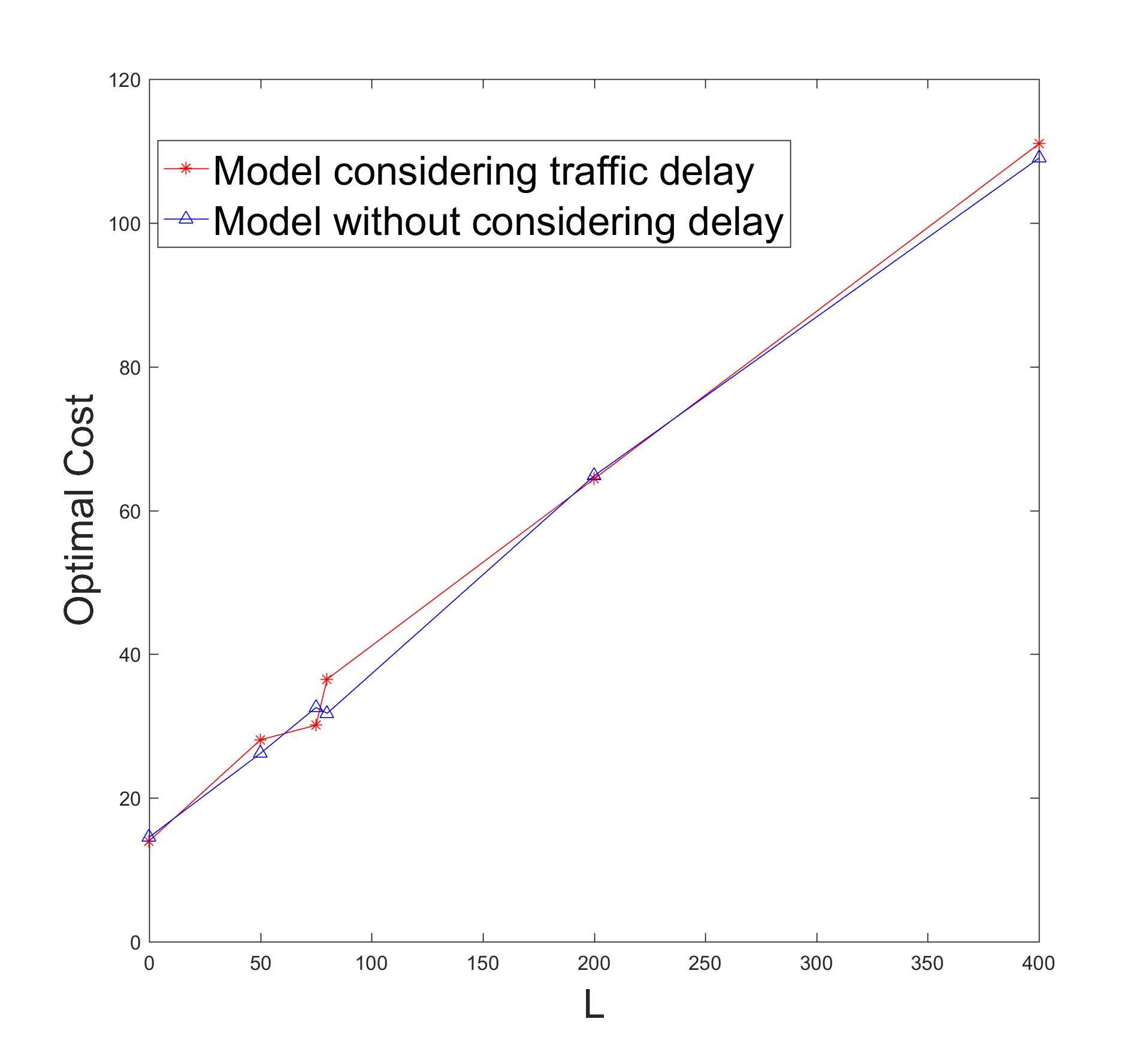
Figure 6: Comparison of Optimal Average Queue Cost vs L.

1. Average Queue Cost Function. We minimize metric (56), over $[0,T]$. All three arrival processes are Poisson with rates $\bar{\alpha}=[0.41,0.45,0.32]$ and the departure rates at roads $1,2,3,4$ are $[1.2,1.3,1.2,1.1]$. We choose $T=1000$s, $w_{i}=1$ and $\theta_{i}\in[10,50]$ for all $i$, and the initial $\theta_{i}$ values are $[40,20,20,40]$. Figure 6 shows the optimal cost (averaged over $10$ sample paths) considering the transit delay in SFM between intersections (red curve) and ignoring this delay (blue curve) as a function of $L$. In this case, delay has no effect on the long term total average queue length, as expected. However, this metric may not accurately capture traffic congestion.

2. Power Cost Function, $P=2$. For the same settings as before and a quadratic queuing cost, Fig. 7 shows how this cost function and the associated controllable parameters converge when $L=100$, achieving a $40\%$ cost decrease. In the left plot of Fig. 8, we use the SFM both including the transit delay and ignoring this delay in order compare the optimal costs under these two models. Clearly, including delays in our IPA estimators for $L>0$ achieves a lower cost, with the gap increasing as $L$ increases.

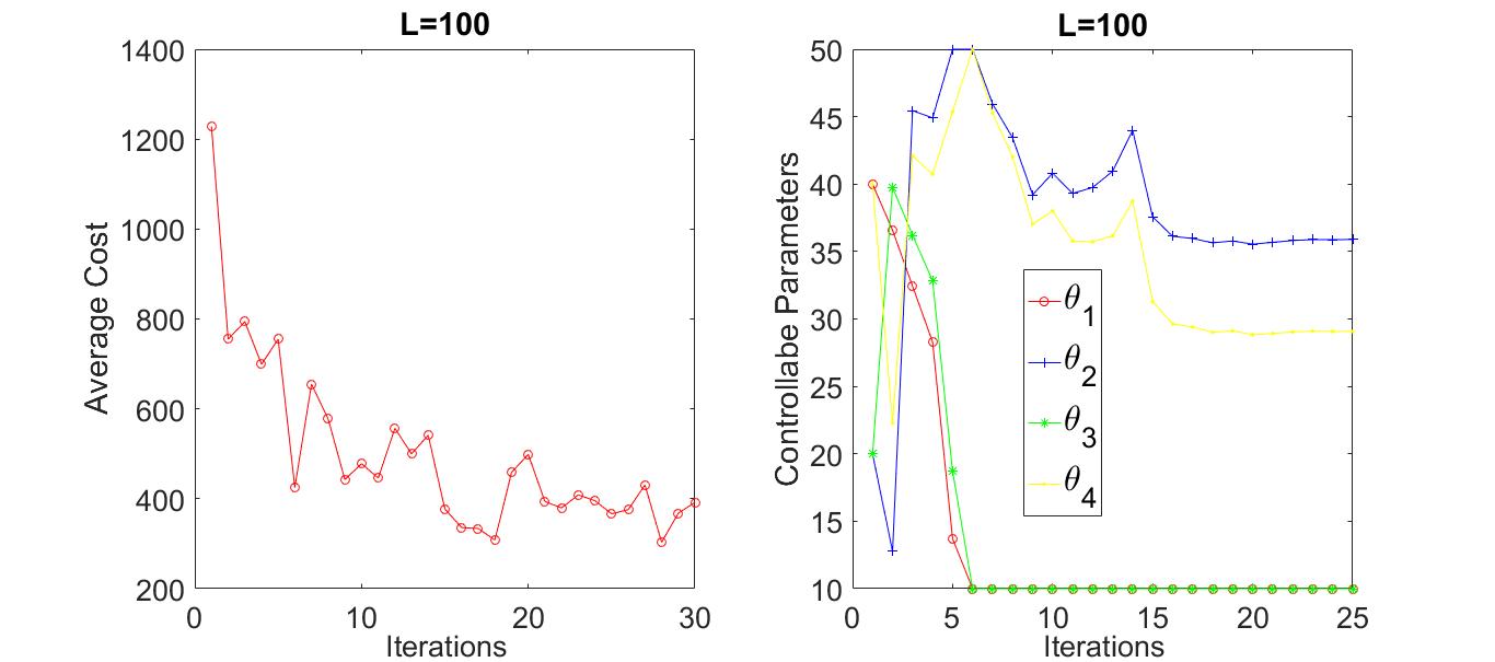
Figure 7: Optimal Power Cost Function vs Iterations.

Figure 8: Comparison of Optimal Cost with/without delay vs $L$.

3. Threshold Cost Function. For the same settings and a common threshold $\zeta_{i}=25$ for all $i$ and with $L=35$, Fig. 9 shows how this cost function and the associate controllable parameters converge, with the cost converging to its zero lower bound, therefore, in this case we see that our approach reaches the global optimum. In the right plot of Fig. 8, we apply the SFM considering both the transit delay between intersections and ignoring this delay so as to compare the resulting optimal costs.Once again, including delays achieves a lower cost, with the gap increasing as $L$ increases.

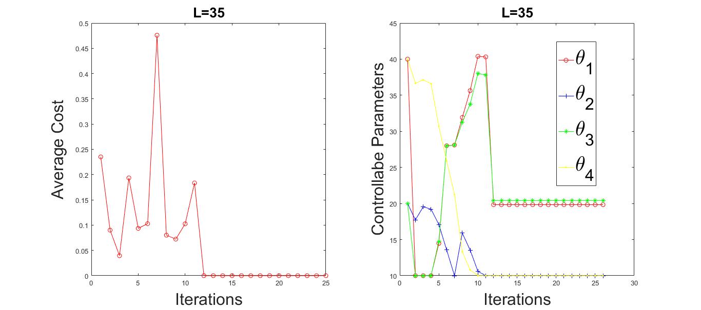
Figure 9: Optimal Threshold Cost Function vs Iterations.

Figure 10: Distribution of queue lengths under $L=35$.

In Fig. 10, we provide histograms of the queue contents when $L=35$. On the left, the controllable parameters are at their initial values $[40,20,20,40]$ and we can see that queues $2$, $3$, and $12$ frequently exceed the threshold. Under the optimal solution we obtain (right side) taking the transit delay between intersections into account, observe that no queue ever exceeds the threshold over $[0,T]$, hence the optimal cost $0$ is obtained. Moreover, note that the probabilities that $x_{2}(t)=0$ and $x_{3}(t)=0$ significantly increase indicating a much improved traffic balance.

6 CONCLUSIONS AND FUTURE WORK

We have extended SFMs to allow for delays which can arise in the flow movement. We have applied this framework to the multi-intersection traffic light control problem by including transit delays for vehicles moving from one intersection to the next and developed IPA for this extended SFM in order to derive on-line gradient estimates of several congestion cost metrics with respect to the controllable green/red cycle lengths, including two new cost metrics that better capture congestion. Our simulation results show that the inclusion of delays in our analysis leads to improved performance relative to models that ignore delays. Future work aims at extensions to allow traffic blocking between intersections and allowing multiple traffic bursts between intersections.

References

- Anderson et al. [2015] Anderson, M.P., Woessner, W.W., and Hunt, R.J. (2015). Applied groundwater modeling: simulation of flow and advective transport. Academic Press.
- Armony et al. [2015] Armony, M., Israelit, S., Mandelbaum, A., Marmor, Y.N., Tseytlin, Y., Yom-Tov, G.B., et al. (2015). On patient flow in hospitals: A data-based queueing-science perspective. Stochastic Systems, 5(1), 146–194.
- Cassandras et al. [2002] Cassandras, C.G., Wardi, Y., Melamed, B., Sun, G., and Panayiotou, C.G. (2002). Perturbation analysis for on-line control and optimization of stochastic fluid models. IEEE Transactions on Automatic Control, 47(8), 1234–1248.
- Cassandras et al. [2010] Cassandras, C.G., Wardi, Y., Panayiotou, C.G., and Yao, C. (2010). Perturbation analysis and optimization of stochastic hybrid systems. European Journal of Control, 6(6), 642–664.
- Cassandras and Lafortune [2009] Cassandras, C.G. and Lafortune, S. (2009). Introduction to discrete event systems. Springer.
- Fleck et al. [2016] Fleck, J.L., Cassandras, C.G., and Geng, Y. (2016). Adaptive quasi-dynamic traffic light control. IEEE Transactions on Control Systems Technology, 24(3), 830–842.
- Fu and Howell [2003] Fu, M.C. and Howell, W.C. (2003). Application of perturbation analysis to traffic light signal timing. Proc. IEEE Conf. on Decision and Control, 4837–4840.
- Geng and Cassandras [2012] Geng, Y. and Cassandras, C.G. (2012). Traffic light control using infinitesimal perturbation analysis. In 2012 IEEE 51st Annual Conf. on Decision and Control (CDC), 7001–7006. IEEE.
- Geng and Cassandras [2015] Geng, Y. and Cassandras, C.G. (2015). Multi-intersection traffic light control with blocking. Discrete Event Dynamic Systems, 25(1-2), 7–30.
- Head et al. [1996] Head, L., Ciarallo, F., and Kaduwela, D.L. (1996). A perturbation analysis approach to traffic signal optimization. INFORMS National Meeting.
- Panayiotou et al. [2005] Panayiotou, C.G., Howell, W.C., and Fu, M.C. (2005). Online traffic light control through gradient estimation usinf stochastic flow models. Proc. IFAC World Congress.
- Wardi et al. [2010] Wardi, Y., Adams, R., and Melamed, B. (2010). A unified approach to infinitesimal perturbation analysis in stochastic flow models: the single-stage case. IEEE Transactions on Automatic Control, 55(1), 89–103.
- Yao and Cassandras [2011] Yao, C. and Cassandras, C.G. (2011). Perturbation analysis of stochastic hybrid systems and applications to resource contention games. Frontiers of Electrical and Electronic Engineering in China, 6(3), 453–467.
- Yin et al. [2013] Yin, S., Ding, S.X., Abandan Sari, A.H., and Hao, H. (2013). Data-driven monitoring for stochastic systems and its application on batch process. Intl. Journal of Systems Science, 44(7), 1366–1376.