Thin obstacle problem:
estimates of the distance to the exact solution

Abstract

We consider elliptic variational inequalities generated by obstacle type problems with thin obstacles. For this class of problems, we deduce estimates of the distance (measured in terms of the natural energy norm) between the exact solution and any function that satisfies the boundary condition and is admissible with respect to the obstacle condition (i.e., it is valid for any approximation regardless of the method by which it was found). Computation of the estimates does not require knowledge of the exact solution and uses only the problem data and an approximation. The estimates provide guaranteed upper bounds of the error (error majorants) and vanish if and only if the approximation coincides with the exact solution. In the last section, the efficiency of error majorants is confirmed by an example, where the exact solution is known.

2010 Mathematics Subject Classification:  Primary 35R35; Secondary 35J20, 65K10.

Keywords: thin obstacle; free boundary problems; variationals problems; estimates of the distance to the exact solution.

1 Introduction

Let $\Omega$ be an open, connected, and bounded domain in $\mathbb{R}^{n}$ with Lipschitz continuous boundary $\partial\Omega$, and let $\mathcal{M}$ be a smooth $(n-1)$-dimensional manifold in $\mathbb{R}^{n}$, which divides $\Omega$ into two Lipschitz subdomains $\Omega_{+}$ and $\Omega_{-}$. Throughout the paper, we use the standard notation for the Lebesgue and Sobolev spaces of functions. Since no confusion may arise, we denote the norm in $L^{2}\left(\Omega\right)$ and the norm in the space $L^{2}\left(\Omega,\mathbb{R}^{n}\right)$ containing vector valued functions by one common symbol $\|\cdot\|_{\Omega}$.

For given functions $\psi:\mathcal{M}\rightarrow\mathbb{R}$ and $\varphi:\partial\Omega\rightarrow\mathbb{R}$ satisfying $\varphi\geq\psi$ on $\mathcal{M}\cap\partial\Omega$, we consider the following variational Problem ($\mathcal{P}$): minimize the functional

$$J(v)=\frac{1}{2}\int\limits_{\Omega}|\nabla v|^{2}dx$$ (1.1)

over the closed convex set

$$\mathbb{K}=\left\{v\in H^{1}\left(\Omega\right):\quad v\geqslant\psi\ \text{on}\ \mathcal{M}\cap\Omega,\quad v=\varphi\ \text{on}\ \partial\Omega\right\}.$$

Here, $\varphi\in H^{1/2}(\partial\Omega)$ and the function $\psi$ is supposed to be smooth.

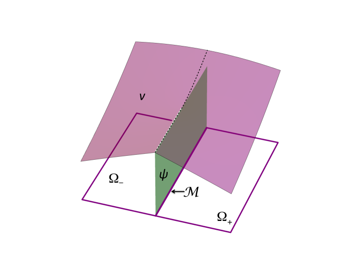
Figure 1: The thin obstacle problem

Problem ($\mathcal{P}$) is called the thin obstacle problem associated with the thin obstacle $\psi$. In many respects, it differs from the classical obstacle problem where the constrain $v\geq\psi$ is imposed on the entire domain $\Omega$. This mathematical model arises in various real life problems. In the $2D$ case (see Fig. 1),  it describes equilibrium of an elastic membrane above a very thin object (e.g., see [KO88]). The well known Signorini problem belongs to the same class of mathematical models. Similar models appear in continuum mechanics, e.g., in temperature control problems and in analysis of flow through semi-permeable walls subject to the phenomenon of osmosis (see, e.g., [DL76]). Thin obstacle problems also arise in financial mathematics if the random variation of an underlying asset changes discontinuously (see [CT04],[Sil07], [PSU12] and the references therein).

The problem ($\mathcal{P}$) is an example of a variational inequality, which mathematical analysis goes back to the fundamental paper [LS67]. Existence of the unique minimizer $u\in\mathbb{K}$ is well known (see [LS67] and also the books [Rod87], [Fri88] and [KS00]). For smooth $\mathcal{M}$ and $\psi$ it is also known that $u\in C^{1,\alpha}_{loc}\left(\Omega_{\pm}\cup\mathcal{M}\right)$ with $0<\alpha\leqslant 1/2$ (see [Caf79], [Ura85], [AC04] and the book [PSU12]). This optimal regularity of $u$ guarantees that $\frac{\partial u\ }{\partial\textbf{n}_{+}}$ and $\frac{\partial u\ }{\partial\textbf{n}_{-}}$ belong to $L^{2}(\mathcal{M})$, where $\textbf{n}_{\pm}$ denote the outer unit normals to $\Omega_{\pm}$ on $\mathcal{M}$. It is also easy to see that the minimizer $u$ satisfies the harmonic equation $\Delta u=0$ in the subdomains $\Omega_{+}$ and $\Omega_{-}$, but in general $u$ is not a harmonic function in $\Omega$. Instead, on $\mathcal{M}$, we have the so-called complimentarity conditions

$$u-\psi\geqslant 0,\qquad\left[\frac{\partial u}{\partial{\mathbf{n}}}\right]\geqslant 0,\qquad(u-\psi)\left[\frac{\partial u}{\partial{\mathbf{n}}}\right]=0,$$ (1.2)

where $\left[\frac{\partial u}{\partial{\mathbf{n}}}\right]:=\frac{\partial u\ }{\partial\textbf{n}_{+}}+\frac{\partial u\ }{\partial\textbf{n}_{-}}$ is the jump of $\nabla u\cdot\mathbf{n}$ across $\mathcal{M}$. Here and later on $\cdot$ denotes the inner product in $\mathbb{R}^{n}$.

Thin obstacle problems have been actively studied from the early 1970s. These studies were mainly focused either on regularity of minimizers (see [Fre75], [Fre77], [Ric78], [Caf79], [Ura85], [AC04], [Gui09]) or on properties of the respective free boundaries (see [Lew72], [ACS08], [CSS08], [GP09], [KPS15], and [DSS16]). A systematic overview of these results can be found in the book [PSU12].

In this paper, we are concerned with a different question. Our analysis is focused not on properties of the exact minimizer, but on estimates of the distance (measured in terms of the natural energy norm) between $u$ and any function $v\in\mathbb{K}$. In other words, we wish to obtain estimates able to detect which neighborhood of $u$ contains a function $v$ (considered as an approximation of the minimizer).

These estimates are fully computable, i.e., they depend only on $v$ (which is assumed to be known) and on the data of the problem ( the exact solution $u$ and the respective exact coincident set $\{u=\psi\}$ do not enter the estimate explicitly). A general approach to the derivation of such type estimates based on methods of the duality theory in the calculus of variations is presented in [Rep00b]. For the classical obstacle problem (which solution is bounded in $\Omega$ from above and below by two obstacles) analogous estimates were obtained in ([Rep00a]). For the two-phase obstacle problem (which was introduced in [Wei01] and studied from regularity point ov view in [Ura01], [SUW04], [SW06], and [SUW07]) similar estimates has been recently derived in [RV15]. These results were obtained by methods of the duality theory in the calculus of variations, which are widely used for analysis of various variational and optimization problems (e.g., see [DL76], [ET76], [IT79], [KS00], [BS00]).

It should be noted that getting explicit estimates of errors is based upon the general relations exposed in [Rep00b], is not at all a straightforwarding and simple matter. In this context, there is a clear difference with the results mentioned above. Indeed, the estimate (2.8) contains an integral term related to the lower dimensional set $\mathcal{M}$. Therefore, our analysis will require estimates with explicitly known constants for the traces of functions on $\mathcal{M}$. For this purpose, we will introduce and analyze an auxiliary variational problem, which generates constants in special Poincaré-type inequalities valid for functions with zero mean boundary traces.

The main results are presented in Theorems 2.1, 2.4, and 3.2, that suggest different majorants of the norm $\|\nabla(v-u)\|_{\Omega}$. The majorants are nonnegative and vanish if and only if $v$ coincides with $u$. Section 4 is devoted to the boundary thin obstacle problem (also known as the scalar Signorini problem). Finally, in the last section we consider an example, where the exact solution of a thin obstacle problem is known. We find the exact distance between this solution and some selected functions $v$ and show that our estimates provide correct upper bounds of the distance.

2 Estimates of the distance to the exact solution

Let $u\in\mathbb{K}$ be a minimizer of variational problem ($\mathcal{P}$). Elementary calculations yield the identity

$$J(v)-J(u)=\frac{1}{2}\|\nabla(v-u)\|_{\Omega}^{2}-\|\nabla u\|_{\Omega}^{2}+\int\limits_{\Omega}\nabla v\cdot\nabla udx,$$

which holds for every $v\in\mathbb{K}$. Since $u$ satisfies the respective variational inequality, we conclude that

$$\frac{1}{2}\|\nabla\left(v-u\right)\|_{\Omega}^{2}\leqslant J(v)-J(u),\qquad\forall v\in\mathbb{K}.$$ (2.1)

The inequality (2.1) does not provide a computable majorant of the distance between $u$ and $v$ because the value $J(u)$ is unknown. Therefore, our goal is to replace the difference $J(v)-J(u)$ in (2.1) by a fully computable quantity.

2.1 The first form of the majorant

For any $\lambda\in\Lambda:=\{\lambda\in L^{2}(\mathcal{M})\,:\,\lambda(x)\geqslant 0\,\text{a.e. on}\,\mathcal{M}\}$, we introduce the perturbed functional

$$J_{\lambda}(v):=J(v)-\int\limits_{\mathcal{M}}\lambda\left(v-\psi\right)d\mu.$$

It is easy to see that

$$\sup\limits_{\lambda\in\Lambda}J_{\lambda}(v)=J(v)-\inf\limits_{\lambda\in\Lambda}\int\limits_{\mathcal{M}}\lambda(v-\psi)d\mu=\left\{\begin{aligned} &J(v),\quad\text{if}\ v\geqslant\psi\ \text{on}\ \mathcal{M},\\ &+\infty,\quad\text{otherwise.}\end{aligned}\right.\quad,$$

Hence,

$$J(u)=\inf\limits_{v\in\mathbb{K}}J(v)=\inf\limits_{v\in\varphi+H^{1}_{0}(\Omega)}\sup\limits_{\lambda\in\Lambda}J_{\lambda}(v),$$ (2.2)

where $\varphi+H^{1}_{0}(\Omega):=\left\{w=\varphi+v:v\in H^{1}_{0}\left(\Omega\right)\right\}$, and $H^{1}_{0}(\Omega)$ is a subspace of $H^{1}(\Omega)$ containing the functions vanishing on the boundary.

The functional $J_{\lambda}$ generates the following variational problem $(\mathcal{P}_{\lambda})$: find $u_{\lambda}\in\varphi+H^{1}_{0}(\Omega)$ such that

$$J_{\lambda}(u_{\lambda}):=\inf\limits_{v\in\varphi+H^{1}_{0}(\Omega)}J_{\lambda}(v).$$ (2.3)

Since $\varphi+H^{1}_{0}(\Omega)$ is the affine subspace of $H^{1}(\Omega)$ and $J_{\lambda}$ is a quadratic functional, the results of [LS67] imply unique solvability of the problem ($\mathcal{P}_{\lambda}$) for any $\lambda\in\Lambda$. Moreover, in view of (2.2), $J(u)$ is bounded from below by the quantity $J_{\lambda}(u_{\lambda})$. Indeed,

$$J(u)=\inf\limits_{v\in\varphi+H^{1}_{0}(\Omega)}\sup\limits_{\lambda\in\Lambda}J_{\lambda}(v)\geqslant\sup\limits_{\lambda\in\Lambda}\inf\limits_{v\in\varphi+H^{1}_{0}(\Omega)}J_{\lambda}(v)\geqslant J_{\lambda}(u_{\lambda})\quad\forall\lambda\in\Lambda.$$ (2.4)

The dual counterpart of ($\mathcal{P}_{\lambda}$) is generated by the Lagrangian

$$\mathcal{L}_{\lambda}(v,y^{*}):=\int\limits_{\Omega}\left(y^{*}\cdot\nabla v-\frac{1}{2}|y^{*}|^{2}\right)dx-\int\limits_{\mathcal{M}}\lambda(v-\psi)d\mu,$$

which is defined on the set $(\varphi+H^{1}_{0}(\Omega))\times L^{2}\left(\Omega,\mathbb{R}^{n}\right)$. Obviously,

$$J_{\lambda}(v)=\sup\limits_{y^{*}\in{L^{2}\left(\Omega,\mathbb{R}^{n}\right)}}\mathcal{L}_{\lambda}(v,y^{*})$$

and the corresponding dual functional $J^{*}_{\lambda}$ is defined by the relation

$$J^{*}_{\lambda}(y^{*}):=\inf\limits_{v\in\varphi+H^{1}_{0}(\Omega)}\mathcal{L}_{\lambda}(v,y^{*}).$$

It is not difficult to see that

$$J^{*}_{\lambda}(y^{*}):=\left\{\begin{aligned} \int\limits_{\Omega}\left(y^{*}\cdot\nabla\varphi-\frac{1}{2}|y^{*}|^{2}\right)dx-\int\limits_{\mathcal{M}}\lambda\left(\varphi-\psi\right)d\mu&\quad\text{if}\quad y^{*}\in Q^{*}_{\lambda,\mathcal{M}},\\ \qquad\qquad-\infty\qquad\qquad\qquad\qquad&\quad\text{if}\quad y^{*}\notin Q^{*}_{\lambda,\mathcal{M}},\end{aligned}\right.$$

where

$$Q^{*}_{\lambda,\mathcal{M}}:=\left\{y^{*}\in{L^{2}\left(\Omega,\mathbb{R}^{n}\right)}:\int\limits_{\Omega}y^{*}\cdot\nabla wdx=\int\limits_{\mathcal{M}}\lambda wd\mu\quad\forall w\in H^{1}_{0}\left(\Omega\right)\right\}.$$

The set $Q^{*}_{\lambda,\mathcal{M}}$ contains functions that satisfy (in the generalized sense) the equation ${\rm div}y^{*}=0$ in $\Omega_{-}$ and $\Omega_{+}$ and the condition $[y^{*}\cdot{\bf n}]=\lambda$ on $\mathcal{M}$ (here $[y^{*}\cdot{\bf n}]$ denotes the jump of $y^{*}\cdot{\bf n}$) . The functional $J^{*}_{\lambda}$ generates a new variational Problem ($\mathcal{P}^{*}_{\lambda}$) (dual to ($\mathcal{P}_{\lambda}$)): find $y_{\lambda}^{*}\in Q^{*}_{\lambda,\mathcal{M}}$ such that

$$J^{*}_{\lambda}(y^{*}_{\lambda}):=\sup\limits_{y^{*}\in Q_{\lambda,\mathcal{M}}}J^{*}_{\lambda}(y^{*}).$$

This is a quadratic maximization problem with a strictly concave and continuous functional. Well known results of convex analysis (see, e.g., [ET76]) guarantee that it has a unique maximizer in the affine subspace $Q^{*}_{\lambda,\mathcal{M}}$. Moreover, we have  the duality relation

$$J_{\lambda}(u_{\lambda})=\inf\limits_{v\in\varphi+H^{1}_{0}(\Omega)}J_{\lambda}(v)=\sup\limits_{y^{*}\in Q^{*}_{\lambda,\mathcal{M}}}J^{*}_{\lambda}(y^{*})=J^{*}_{\lambda}(y^{*}_{\lambda}).$$ (2.5)

Combining (2.4) and (2.5), we deduce the estimate

$$J(v)-J(u) \leqslant J(v)-J^{*}_{\lambda}(y^{*}_{\lambda})=J(v)-\sup\limits_{y^{*}\in Q^{*}_{\lambda,\mathcal{M}}}J^{*}_{\lambda}(y^{*})$$

$$=J(v)+\inf\limits_{y^{*}\in Q^{*}_{\lambda,\mathcal{M}}}\left(-J^{*}_{\lambda}(y^{*})\right)=\inf\limits_{y^{*}\in Q^{*}_{\lambda,\mathcal{M}}}\left[J(v)-J^{*}_{\lambda}(y^{*})\right].$$

Therefore, the inequality

$$J(v)-J(u)\leqslant J(v)-J^{*}_{\lambda}(y^{*})$$ (2.6)

holds true for all $v\in\mathbb{K}$, all $\lambda\in\Lambda$, and all $y^{*}\in Q^{*}_{\lambda,\mathcal{M}}$.

Thanks to the assumption $\varphi\in H^{1/2}(\partial\Omega)$, the boundary datum $\varphi$ allows a continuation as $H^{1}$-function on the whole set $\Omega$. We will preserve the notation $\varphi$ for the extended function. Since $y^{*}\in Q^{*}_{\lambda,\mathcal{M}}$ and $v-\varphi\in H^{1}_{0}(\Omega)$ for any $v\in\mathbb{K}$, we find that

$$\int\limits_{\Omega}y^{*}\cdot\nabla\varphi dx=\int\limits_{\Omega}y^{*}\cdot\nabla vdx-\int\limits_{\Omega}y^{*}\cdot\nabla(v-\varphi)dx=\int\limits_{\Omega}y^{*}\cdot\nabla vdx-\int\limits_{\mathcal{M}}\lambda(v-\varphi)d\mu.$$

Now the right-hand side of (2.6) can be rewritten as follows:

$$J(v)-J^{*}_{\lambda}(y^{*})=\int\limits_{\Omega}\left(\frac{1}{2}|\nabla v|^{2}+\frac{1}{2}|y^{*}|^{2}-y^{*}\cdot\nabla\varphi\right)dx+\int\limits_{\mathcal{M}}\lambda(\varphi-\psi)d\mu\\ =\frac{1}{2}\int\limits_{\Omega}|\nabla v-y^{*}|^{2}dx+\int\limits_{\mathcal{M}}\lambda\left(v-\psi\right)d\mu.$$ (2.7)

Combination of (2.1), (2.6) and (2.7) yields the following upper bound of the error:

Theorem 2.1.

For any $v\in\mathbb{K}$, the distance to the minimizer $u$ is subject to the estimate

$$\|\nabla(v-u)\|_{\Omega}^{2}\leqslant\|\nabla v-y^{*}\|^{2}_{\Omega}+2\int\limits_{\mathcal{M}}\lambda\left(v-\psi\right)d\mu,$$ (2.8)

where $\lambda$ and $y^{*}$ are arbitrary functions in $\Lambda$ and $Q^{*}_{\lambda,\mathcal{M}}$, respectively.

Theorem 2.1 can be viewed as a generalized form of the hypercircle estimate (see [PS47] and [Mik64]) for the considered class of problems.

Remark 2.2.

Define the coincidence sets associated with $u$ and $v$:

$${\mathcal{M}}^{u}_{\psi}:=\{x\in{\mathcal{M}}\,:\,u(x)=\psi(x)\,\}\qquad{\rm and}\qquad{\mathcal{M}}^{v}_{\psi}:=\{x\in{\mathcal{M}}\,:\,v(x)=\psi(x)\,\}.$$

Assume that ${\mathcal{M}}^{u}_{\psi}\subset{\mathcal{M}}^{v}_{\psi}$. In this case, the estimate (2.8) is sharp in the sense that there exist $y^{*}$ and $\lambda$ such that the inequality holds as the equality. Indeed, let $y^{*}=p^{*}:=\nabla u$ and $\lambda_{*}=\left[p^{*}\cdot{\bf n}\right]$. Evidently, $p^{*}\in Q^{*}_{\lambda_{*},\mathcal{M}}$. In view of (1.2), $\lambda_{*}=0$ on $\mathcal{M}\setminus{\mathcal{M}}^{u}_{\psi}$. Since $\mathcal{M}\setminus{\mathcal{M}}^{v}_{\psi}\subset\mathcal{M}\setminus{\mathcal{M}}^{u}_{\psi}$, we conclude that

$$\int\limits_{\mathcal{M}}\lambda_{*}\left(v-\psi\right)d\mu=\int\limits_{\mathcal{M}\setminus{\mathcal{M}}^{v}_{\psi}}\lambda_{*}\left(v-\psi\right)d\mu=0.$$

Hence, the right hand side of (2.8) coincides with the left one.

2.2 Advanced forms of the majorant

Inequality (2.8) provides a simple and transparent form of the upper bound, but it operates with the set $Q^{*}_{\lambda,\mathcal{M}}$, which is defined by means of differential type conditions. This set is rather narrow and inconvenient if we wish to use simple approximations. In this section, we overcome this drawback and replace (2.8) by a more general estimate valid for functions in the set

$$H\left(\Omega_{\pm},\text{\rm{div}}\right):=\left\{q^{*}\in L^{2}\left(\Omega,\mathbb{R}^{n}\right):\text{\rm{div}}\,(q^{*}|_{\Omega_{\pm}})\in L^{2}\left(\Omega_{\pm}\right),\;\left[q^{*}\cdot\mathbf{n}\right]\in L^{2}({\mathcal{M}})\right\},$$

which is much wider than $Q^{*}_{\lambda,\mathcal{M}}$.

Lemma 2.3.

Let $q^{*}\in H(\Omega_{\pm},\text{\rm{div}})$, and let $\lambda\in\Lambda$. Then

$$\inf\limits_{y^{*}\in Q^{*}_{\lambda,\mathcal{M}}}\|q^{*}-y^{*}\|_{\Omega} \leqslant C_{F_{\Omega_{+}}}\|\text{\rm{div}}\,q^{*}\|_{\Omega_{+}}+C_{F_{\Omega_{-}}}\|\text{\rm{div}}\,q^{*}\|_{\Omega_{-}}$$ (2.9)

$$+C_{Tr_{\mathcal{M}}}\|\lambda-[q^{*}\cdot\mathbf{n}]\|_{\mathcal{M}},$$

where $C_{Tr_{\mathcal{M}}}$ and $C_{F_{\Omega_{\pm}}}$ are the constants defined by (2.13) and (2.14), respectively.

Proof.

Consider an auxiliary variational problem ($\mathcal{P}_{q^{*}})$: minimize the functional

$$\mathcal{J}_{q^{*}}(w)=\int\limits_{\Omega}\left(\frac{1}{2}|\nabla w|^{2}+q^{*}\cdot\nabla w\right)dx-\int\limits_{\mathcal{M}}\lambda wd\mu$$

on the space $H^{1}_{0}(\Omega)$. For any given $q^{*}\in H(\Omega_{\pm},\text{\rm{div}})$ and $\lambda\in\Lambda$, the functional $\mathcal{J}_{q^{*}}$ is convex, continuous, and coercive on $H^{1}_{0}(\Omega)$. Hence the problem $\mathcal{P}_{q^{*}}$ has a unique minimizer $w_{\lambda,q^{*}}\in H^{1}_{0}$ .

Since $q^{*}\in H\left(\Omega_{\pm},\text{\rm{div}}\right)$, the functional $\mathcal{J}_{q^{*}}$ has the form

$$\mathcal{J}_{q^{*}}(w) =\int\limits_{\Omega}\frac{1}{2}|\nabla w|^{2}dx-\int\limits_{\Omega_{+}}w\text{\rm{div}}\,q^{*}dx-\int\limits_{\Omega_{-}}w\text{\rm{div}}\,q^{*}dx$$ (2.10)

$$-\int\limits_{\mathcal{M}}\left(\lambda-[q^{*}\cdot\mathbf{n}]\right)wd\mu.$$

For any $\widetilde{w}\in H^{1}_{0}(\Omega)$, the minimizer $w_{\lambda,q^{*}}$ satisfies the identity

$$\int\limits_{\Omega}\nabla w_{\lambda,q^{*}}\cdot\nabla\widetilde{w}dx=\int\limits_{\Omega_{+}}\widetilde{w}\text{\rm{div}}\,q^{*}dx+\int\limits_{\Omega_{-}}\widetilde{w}\text{\rm{div}}\,q^{*}dx+\int\limits_{\mathcal{M}}\left(\lambda-\left[q^{*}\cdot\mathbf{n}\right]\right)\widetilde{w}d\mu.$$ (2.11)

We set $\widetilde{w}=w_{\lambda,q^{*}}$ and use the estimate

$$\int\limits_{\mathcal{M}}\left(\lambda-\left[q^{*}\cdot\mathbf{n}\right]\right)w_{\lambda,q^{*}}d\mu \leqslant C_{Tr_{\mathcal{M}}}(\Omega_{\pm})\|\nabla w_{\lambda,q^{*}}\|_{\Omega_{\pm}}\,\|\lambda-\left[q^{*}\cdot\mathbf{n}\right]\|_{\mathcal{M}}$$ (2.12)

$$\leqslant C_{Tr_{\mathcal{M}}}\|\nabla w_{\lambda,q^{*}}\|_{\Omega}\,\|\lambda-\left[q^{*}\cdot\mathbf{n}\right]\|_{\mathcal{M}},$$

where

$$C_{Tr_{\mathcal{M}}}:=\min\{C_{Tr_{\mathcal{M}}}(\Omega_{+}),C_{Tr_{\mathcal{M}}}(\Omega_{-})\}$$ (2.13)

and the constants come from the trace inequalities

$$\|w\|_{\mathcal{M}}\leqslant C_{Tr_{\mathcal{M}}}(\Omega_{\pm})\|\nabla w\|_{\Omega_{\pm}}.$$

Two other terms in the right hand side of (2.11) are estimated by the Friedrich’s type inequalities

$$\|w\|_{\Omega_{\pm}}\leqslant C_{F_{\Omega_{\pm}}}\|\nabla w\|_{\Omega_{\pm}}.$$ (2.14)

Thus, (2.11) and (2.12) yield the estimate

$$\|\nabla w_{\lambda,q^{*}}\|_{\Omega}\leqslant C_{F_{\Omega_{+}}}\|\text{\rm{div}}\,q^{*}\|_{\Omega_{+}}+C_{F_{\Omega_{-}}}\|\text{\rm{div}}\,q^{*}\|_{\Omega_{-}}+C_{Tr_{\mathcal{M}}}\|\lambda-\left[q^{*}\cdot\mathbf{n}\right]\|_{\mathcal{M}}.$$ (2.15)

Notice that (2.11) implies the identity

$$\int\limits_{\Omega}\left(\nabla w_{\lambda,q^{*}}+q^{*}\right)\cdot\nabla\widetilde{w}dx=\int\limits_{\mathcal{M}}\lambda\widetilde{w}d\mu\qquad\forall\widetilde{w}\in H^{1}_{0}(\Omega),$$

which shows that the function $\tau^{*}:=\nabla w_{\lambda,q^{*}}+q^{*}\in Q^{*}_{\lambda,\mathcal{M}}$. Hence

$$\inf\limits_{y^{*}\in Q^{*}_{\lambda,\mathcal{M}}}\|q^{*}-y^{*}\|_{\Omega}\leqslant\|q^{*}-\tau^{*}\|_{\Omega}=\|\nabla w_{\lambda,q^{*}}\|_{\Omega}.$$

Now (2.9) follows from (2.15). ∎

Let $q^{*}\in H(\Omega_{\pm},\text{\rm{div}})$, and let $\lambda\in\Lambda$. For any $v\in\mathbb{K}$ and $y^{*}\in Q^{*}_{\lambda,\mathcal{M}}$ we have

$$\|\nabla v-y^{*}\|_{\Omega}\leqslant\|\nabla v-q^{*}\|_{\Omega}+\|q^{*}-y^{*}\|_{\Omega}.$$ (2.16)

By (2.8), (2.16), and (2.9), we obtain the first advanced form of the error majorant:

Theorem 2.4.

For any $v\in\mathbb{K}$, the distance to the minimizer $u$ is subject to the estimate

$$\|\nabla(v-u)\|_{\Omega}\leqslant\mathfrak{M}(v,q^{*},\lambda,\psi),$$ (2.17)

where

$$\mathfrak{M}(v,q^{*},\lambda, \psi):=\|\nabla v-q^{*}\|_{\Omega}+\sqrt{2}\left(\,\int\limits_{\mathcal{M}}\lambda(v-\psi)d\mu\right)^{1/2}$$

$$+C_{F_{\Omega_{+}}}\|\text{\rm{div}}\,q^{*}\|_{\Omega_{+}}+C_{F_{\Omega_{-}}}\|\text{\rm{div}}\,q^{*}\|_{\Omega_{-}}+C_{Tr_{\mathcal{M}}}\|\lambda-[q^{*}\cdot\mathbf{n}]\|_{\mathcal{M}},$$

$\lambda\in\Lambda$, $q^{*}$ is an arbitrary function in $H(\Omega_{\pm},\text{\rm{div}})$, $C_{F_{\Omega_{+}}}$, $C_{F_{\Omega_{-}}}$, and $C_{Tr_{\mathcal{M}}}$ are the same constants as in Lemma 2.3.

In (2.17), the function $q^{*}$ is defined in a much wider set of functions defined without differential relations. The majorant $\mathfrak{M}$ is a nonnegative functional, which vanishes if and only if $v=u$ and $q^{*}=\nabla u$ almost everywhere in $\Omega$, and $\lambda=\lambda_{*}:=\left[\frac{\partial u}{\partial{\mathbf{n}}}\right]$ almost everywhere on $\mathcal{M}$.

Remark 2.5.

By the same arguments as in Remark 2.2, we can prove that the majorant $\mathfrak{M}(v,q^{*},\lambda,\psi)$ is sharp if ${\mathcal{M}}^{u}_{\psi}\subset{\mathcal{M}}^{v}_{\psi}$.

It is useful to have also a modified version of (2.17), which follows from (2.8), (2.16), and Young’s inequalities (with the parameters $\beta_{1}$ and $\beta_{2}$).

Corollary 2.6.

For any $v\in\mathbb{K}$, $\beta_{1}>0$, $\beta_{2}>0$, $q^{*}\in H(\Omega_{\pm},\text{\rm{div}})$, and $\lambda\in\Lambda$, we have

$$\|\nabla(v-u)\|^{2}_{\Omega}\leqslant\mathfrak{M}_{1}(v,q^{*},\beta_{1},\beta_{2})+\mathfrak{M}_{2}(v,q^{*},\beta_{1},\beta_{2}\lambda,\psi),$$ (2.18)

where

$$\mathfrak{M}_{1}(v,q^{*},\beta_{1},\beta_{2}): =(1+\beta_{1})\|\nabla v-q^{*}\|^{2}_{\Omega}\qquad\qquad\qquad\qquad$$

$$+(1+\beta_{1}^{-1}) (1+\beta_{2})\left[C_{F_{\Omega_{+}}}\|\text{\rm{div}}\,q^{*}\|_{\Omega_{+}}+C_{F_{\Omega_{-}}}\|\text{\rm{div}}\,q^{*}\|_{\Omega_{-}}\right]^{2},$$

$$\mathfrak{M}_{2}(v,q^{*},\beta_{1},\beta_{2},\lambda,\psi): =(1+\beta_{1}^{-1})(1+\beta_{2}^{-1})C^{2}_{Tr_{\mathcal{M}}}\|\lambda-\left[q^{*}\cdot\mathbf{n}\right]\|^{2}_{\mathcal{M}}$$

$$+2\int\limits_{\mathcal{M}}\lambda(v-\psi)d\mu,$$

and the constants $C_{F_{\Omega_{+}}}$, $C_{F_{\Omega_{-}}}$, and $C_{Tr_{\mathcal{M}}}$ are the same as in Lemma 2.3.

The majorant (2.18) contains parameters and free functions that can be selected arbitrarily in the respective sets. Below we deduce a new form of (2.18) where the function $\lambda$ will be chosen in the optimal way.

First, we optimize $\mathfrak{M}_{2}$ with respect to $\lambda$. The respective minimization problem is reduced to

$$\inf\limits_{\lambda\in\Lambda}\mathfrak{M}_{2}=c^{-1}_{\beta}\inf\limits_{\lambda\in\Lambda}\int\limits_{\mathcal{M}}\left(C^{2}_{Tr_{\mathcal{M}}}(\lambda-\left[q^{*}\cdot\mathbf{n}\right])^{2}+2\lambda c_{\beta}(v-\psi)\right)d\mu,$$

where $c_{\beta}:=\beta_{1}\beta_{2}(1+\beta_{1})^{-1}(1+\beta_{2})^{-1}$. The corresponding Euler-Lagrange equation has the form

$$2C^{2}_{Tr_{\mathcal{M}}}(\lambda-\left[q^{*}\cdot\mathbf{n}\right])+2c_{\beta}(v-\psi)=0.$$

From here, taking into account the condition $\lambda\geqslant 0$ a.e. on $\mathcal{M}$, we find the minimizer

$$\overline{\lambda}=\left\{\begin{aligned} \left[q^{*}\cdot\mathbf{n}\right]-&c_{\beta}C^{-2}_{Tr_{\mathcal{M}}}(v-\psi),\quad\ \text{if}\ \left[q^{*}\cdot\mathbf{n}\right]\geqslant c_{\beta}C^{-2}_{Tr_{\mathcal{M}}}(v-\psi),\\ &0,\qquad\qquad\qquad\quad\ \text{if}\ \left[q^{*}\cdot\mathbf{n}\right]<c_{\beta}C^{-2}_{Tr_{\mathcal{M}}}(v-\psi).\end{aligned}\right.$$

Plugging $\overline{\lambda}$ in the right-hand side of (2.18) implies the following result.

Theorem 2.7.

For any $v\in\mathbb{K}$,

$$\|\nabla(v-u)\|^{2}_{\Omega}\leqslant\mathfrak{M}_{1}(v,q^{*},\beta_{1},\beta_{2})+\mathfrak{M}_{3}(v,q^{*},\beta_{1},\beta_{2},\psi),$$ (2.19)

where $q^{*}$ is an arbitrary function in $H(\Omega_{\pm},\text{\rm{div}})$, $\beta_{1}$ and $\beta_{2}$ are arbitrary nonegative numbers, $\mathfrak{M}_{1}$ is the same as in (2.18),

$$\mathfrak{M}_{3}(v,q^{*},\beta_{1},\beta_{2},\psi):=\int\limits_{\mathcal{M}}\rho(v,q^{*},c_{\beta},\psi)d\mu,$$

and

$$\rho(v,q^{*},c_{\beta},\psi):=\left\{\begin{aligned} (v-\psi)\big{(}2\left[q^{*}\cdot\mathbf{n}\right]-\frac{c_{\beta}}{C^{2}_{Tr_{\mathcal{M}}}}(v-\psi)\big{)},\ &\text{if}\ \left[q^{*}\cdot\mathbf{n}\right]\geqslant\frac{c_{\beta}}{C^{2}_{Tr_{\mathcal{M}}}}(v-\psi),\\ \frac{C^{2}_{Tr_{\mathcal{M}}}}{c_{\beta}}\left[q^{*}\cdot\mathbf{n}\right]^{2},\qquad\qquad\ \ \ \ \quad&\text{if}\ \left[q^{*}\cdot\mathbf{n}\right]<\frac{c_{\beta}}{C^{2}_{Tr_{\mathcal{M}}}}(v-\psi).\end{aligned}\right.$$

It is clear that the quantities $\mathfrak{M}_{1}$ and $\mathfrak{M}_{3}$ are always nonnegative and the functional $\mathfrak{M}_{4}~{}:=~{}\mathfrak{M}_{1}~{}+\mathfrak{M}_{3}$ satisfies for any $\beta_{1},\beta_{2}>0$ the relation

$$\mathfrak{M}_{4}(u,\nabla u,\beta_{1},\beta_{2},\psi)=0.$$

On the other hand, if $\mathfrak{M}_{4}(v,q^{*},\beta_{1},\beta_{2},\psi)=0$ then $v=u$ almost everywhere in $\Omega$. Moreover, in this case the conditions

$$q^{*} =\nabla u\quad\text{a.e. in}\ \Omega,$$ (2.20)

$$\Delta u =0\qquad\text{a.e. in}\ \Omega_{\pm},$$

$$(u-\psi)\left[\nabla u\cdot\mathbf{n}\right] =0\qquad\text{a.e. on}\ \mathcal{M}$$

hold true. We point out that the third equality in (2.20) is provided by strict positivity of the factor $2\left[q^{*}\cdot\mathbf{n}\right]-\frac{c_{\beta}}{C^{2}_{Tr_{\mathcal{M}}}}(v-\psi)$ in definition of $\rho$. Therefore, one can conclude that the majorant $\mathfrak{M}_{4}$ vanishes if and only if $v=u$ and $q^{*}=\nabla u$ almost everywhere in $\Omega$.

Remark 2.8.

Applying the same arguments as in Remark 2.2, we can prove that the majorant $\mathfrak{M}_{4}(v,q^{*},\beta_{1},\beta_{2},\psi)$ is sharp if ${\mathcal{M}}^{u}_{\psi}\subset{\mathcal{M}}^{v}_{\psi}$.

One can also prove that for any $\beta_{1},\beta_{2}>0$, the functional $\mathfrak{M}_{4}(v,q^{*},\beta_{1},\beta_{2},\psi)$ possesses necessary continuity properties with respect to the first and second arguments. Thus,

$$\mathfrak{M}_{4}(v_{k},q^{*}_{k},\beta_{1},\beta_{2},\psi)\to 0$$

if $v_{k}\to u$ in $\mathbb{K}$ and $q^{*}_{k}\to\nabla u$ in $L^{2}(\Omega_{\pm})$ and $\left[q_{k}^{*}\cdot\mathbf{n}\right]\to\left[\nabla u\cdot\mathbf{n}\right]$ in $L^{2}(\mathcal{M})$. Thus, taking into account Remark 2.8, we conclude that the estimate (2.19) has no gap between the left and right hand sides and we can always select the parameters of $\mathfrak{M}_{4}$ such that it is arbitrary close to the energy norm of the error.

3 Estimates with explicit constants

It should be also noted that for complicated domains the constants $C_{F_{\Omega_{\pm}}}$ and $C_{Tr_{\mathcal{M}}}(\Omega_{\pm})$ entering above derived estimates (2.17)-(2.19) may be unknown. In this case, we need to find guaranteed and realistic upper bounds of them. Depending on a particular domain, this task may be fairly easy or very difficult. It is therefore of interest to look at other variants of Lemma 2.3, which operates with different constants. In this section, we establish another estimate based on the Poincaré inequlity for functions having zero mean values in $\Omega_{\pm}$ and on the so–called ”sloshing” inequality for functions with zero mean traces on $\mathcal{M}$. As a result, we obtain estimates of the distance to the minimizer $u$ containing the constants which are either explicitly known or easily definable.

Henceforth, we denote by $\left\{\!\left|\,w\,\right|\!\right\}_{\omega}$ the mean value of $w$ on the set $\omega$. In view of the Poincare inequality

$$\|w\|_{\Omega_{\pm}}\leq C_{P_{\Omega_{\pm}}}\|\nabla w\|_{\Omega_{\pm}}\qquad\forall w\in\widetilde{H}^{1}(\Omega_{\pm}):=\left\{w\in H^{1}(\Omega_{\pm})\,:\,\left\{\!\left|\,w\,\right|\!\right\}_{\Omega_{\pm}}=0\right\}.$$ (3.1)

Similar inequalities hold for the functions defined in $\Omega_{+}$ and $\Omega_{-}$ having zero mean values on $\mathcal{M}$:

$$\|w\|_{\mathcal{M}}\leq C_{P_{\mathcal{M}}}(\Omega_{\pm})\|\nabla w\|_{\Omega_{\pm}}\qquad\forall w\in\widetilde{H}^{1}_{\mathcal{M}}(\Omega_{\pm}):=\left\{w\in H^{1}(\Omega_{\pm})\,:\,\left\{\!\left|\,w\,\right|\!\right\}_{\mathcal{M}}=0\right\}.$$ (3.2)

Lemma 3.1.

Let $q^{*}\in H(\Omega_{\pm},\text{\rm{div}})$ and $\lambda\in\Lambda$ satisfy the following additional conditions:

$$\int\limits_{\Omega_{+}}\text{\rm{div}}\,q^{*}dx=\int\limits_{\Omega_{-}}\text{\rm{\rm{div}}}\,q^{*}dx=0\qquad{\rm and}\qquad\int\limits_{\mathcal{M}}(\lambda-\left[q^{*}\cdot\mathbf{n}\right])d\mu=0.$$ (3.3)

Then, for any $\alpha\in[0,1]$, we have

$$\inf\limits_{y^{*}\in Q^{*}_{\lambda,\mathcal{M}}}\|q^{*}-y^{*}\|^{2}_{\Omega}\leqslant(\mathfrak{D}_{-}(q^{*})+\alpha\mathfrak{m}_{-}(q^{*}))^{2}+(\mathfrak{D}_{+}(q^{*})+(1-\alpha)\mathfrak{m}_{+}(q^{*}))^{2},$$ (3.4)

where $\mathfrak{D}_{\pm}(q^{*}):=C_{P_{\Omega_{\pm}}}\|\text{\rm{div}}\,q^{*}\|_{\Omega_{\pm}}$ and $\mathfrak{m}_{\pm}(q^{*})=C_{P_{\mathcal{M}}}(\Omega_{\pm})\|\lambda-[q^{*}\cdot\mathbf{n}]\|_{\mathcal{M}}$.

Proof.

We use the same arguments as in the proof of Lemma 2.3 and arrive at the identity (2.11). In view of (3.3), this identity implies the relation

$$\|\nabla w_{\lambda,q^{*}}\|^{2}_{\Omega} =\int\limits_{\Omega_{+}}\left(w_{\lambda,q^{*}}-\{w_{\lambda,q^{*}}\}_{\Omega_{+}}\right)\text{\rm{div}}\,q^{*}dx$$

$$+\int\limits_{\Omega_{-}}\left(w_{\lambda,q^{*}}-\{w_{\lambda,q^{*}}\}_{\Omega_{-}}\right)\text{\rm{div}}\,q^{*}dx$$

$$+\int\limits_{\mathcal{M}}(\lambda-\left[q^{*}\cdot\mathbf{n}\right])\left(w_{\lambda,q^{*}}-\{w_{\lambda,q^{*}}\}_{\mathcal{M}}\right)d\mu.$$

By (3.1) and (3.2), we obtain

$$\int\limits_{\Omega_{\pm}}\left(w_{\lambda,q^{*}}-\{w_{\lambda,q^{*}}\}_{\Omega_{+}}\right)\text{\rm{div}}\,q^{*}dx\leqslant C_{P_{\Omega_{\pm}}}\|\nabla w_{\lambda,q^{*}}\|_{\Omega_{\pm}}\|\text{\rm{div}}\,q^{*}\|_{\Omega_{\pm}},$$

$$\int\limits_{\mathcal{M}}(\lambda-\left[q^{*}\cdot\mathbf{n}\right])\left(w_{\lambda,q^{*}}-\{w_{\lambda,q^{*}}\}_{\mathcal{M}}\right)d\mu\leqslant C_{P_{\mathcal{M}}}(\Omega_{\pm})\|\nabla w_{\lambda,q^{*}}\|_{\Omega_{\pm}}\|\lambda-[q^{*}\cdot\mathbf{n}]\|_{\mathcal{M}}.$$

Then,

$$\|\nabla w_{\lambda,q^{*}}\|^{2}_{\Omega} \leqslant\mathfrak{D}_{-}(q^{*})\|\nabla w_{\lambda,q^{*}}\|_{\Omega_{-}}+\mathfrak{D}_{+}(q^{*})\|\nabla w_{\lambda,q^{*}}\|_{\Omega_{+}}+\alpha\mathfrak{m}_{-}(q^{*})\|\nabla w_{\lambda,q^{*}}\|_{\Omega_{-}}$$ (3.5)

$$+(1-\alpha)\mathfrak{m}_{+}(q^{*})\|\nabla w_{\lambda,q^{*}}\|_{\Omega_{+}}$$

$$\leqslant\left((\mathfrak{D}_{-}(q^{*})+\alpha\mathfrak{m}_{-}(q^{*}))^{2}+(\mathfrak{D}_{+}(q^{*})+(1-\alpha)\mathfrak{m}_{+}(q^{*}))^{2}\right)^{1/2}\|\nabla w_{\lambda,q^{*}}\|_{\Omega}.$$

Using (3.5) and repeating the same arguments as at the end of the proof of Lemma 2.3, we arrive at (3.4). ∎

The quantities $\mathfrak{D}_{\pm}(q^{*})$ contain the Poincaré constants for $\Omega_{\pm}$. If these domains are convex, then due to the estimate of Payne and Weinberger (see [PW60]) we know that

$$C_{P_{\Omega_{\pm}}}\leqslant\frac{\text{diam}\,\Omega_{\pm}}{\pi}.$$

The constants $C_{P_{\mathcal{M}}}(\Omega_{\pm})$ entering $\mathfrak{m}_{\pm}(q^{*})$ are also easy to estimate. These constants are known for triangles (see [NR15] and [MR16]). Due to this fact, we can easily obtain upper bounds of the constants for a wide collection of domains.

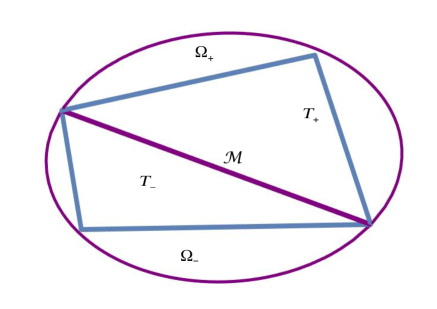
Figure 2: Triangles $T_{+}$ and $T_{-}$

Indeed, let $T_{+}\subset\Omega_{+}$ and $\mathcal{M}$ as a face of this triangle (see Fig. 2). It is clear that

$$\|w\|_{\mathcal{M}}\leqslant C_{P_{\mathcal{M}}}(T_{+})\|\nabla w\|_{T_{+}}\leqslant C_{P_{\mathcal{M}}}(T_{+})\|\nabla w\|_{\Omega_{+}}\qquad\forall w\in\widetilde{H}^{1}_{\mathcal{M}}(\Omega_{+}),$$

and we can use the constant $C_{P_{\mathcal{M}}}(T_{+})$ as an upper bound of $C_{P_{\mathcal{M}}}(\Omega_{+})$.

Lemma 3.1, (2.8), and (2.16) yield the following majorant of the distance to $u$.

Theorem 3.2.

Let $u\in\mathbb{K}$ be a minimizer of variational problem ($\mathcal{P}$). Let $q^{*}\in H(\Omega_{+},\Omega_{-},\text{\rm{div}})$, and let the conditions (3.3) be satisfied. Then, for any $v\in\mathbb{K}$, $\alpha\in[0,1]$, and $\lambda\in\Lambda$, the upper bound of error is given by the estimate

$$\|\nabla(v-u)\|_{\Omega}\leqslant\mathfrak{M}_{5}(v,q^{*},\alpha,\lambda,\psi),$$ (3.6)

where

$$\mathfrak{M}_{5}(v,q^{*},\alpha,\lambda,\psi) :=\|\nabla v-q^{*}\|_{\Omega}+\sqrt{2}\left(\int\limits_{\mathcal{M}}\lambda(v-\psi)d\mu\right)^{1/2}$$

$$+\left((\mathfrak{D}_{-}(q^{*})+\alpha\mathfrak{m}_{-}(q^{*}))^{2}+(\mathfrak{D}_{+}(q^{*})+(1-\alpha)\mathfrak{m}_{+}(q^{*}))^{2}\right)^{1/2},$$

where the functionals $\mathfrak{D}_{\pm}(q^{*})$ and $\mathfrak{m}_{\pm}(q^{*})$ are the same as in Lemma 3.1.

As in Section 2, it is easy to see that the majorant $\mathfrak{M}_{5}$ is a nonnegative function of its arguments, which vanishes if and only if $v=u$ and $q^{*}=\nabla u$ a. e. in $\Omega$, and $\lambda=\left[\frac{\partial u}{\partial{\mathbf{n}}}\right]$ a. e. on $\mathcal{M}$.

Remark 3.3.

The majorant $\mathfrak{M}_{5}(v,q^{*},\alpha,\lambda,\psi)$ is sharp if ${\mathcal{M}}^{u}_{\psi}\subset{\mathcal{M}}^{v}_{\psi}$. The proof is based on the same arguments as in Remark 2.2.

Remark 3.4.

Other forms of the majorant arise if the conditions (3.3) are satisfied only partially. For example, if only the condition

$$\int\limits_{\mathcal{M}}(\lambda-\left[q^{*}\cdot\mathbf{n}\right])d\mu=0$$ (3.7)

is satisfied, then the estimate (3.6) holds true for any $q^{*}\in H(\Omega_{\pm},\text{\rm{div}})$ satisfying (3.7), where the functionals $\mathcal{D}_{-}(q^{*})$ and $\mathcal{D}_{+}(q^{*})$ in $\mathfrak{M}_{3}$ are replaced by $C_{F_{\Omega_{-}}}\|\text{\rm{div}}\,q^{*}\|_{\Omega_{-}}$ and $C_{F_{\Omega_{+}}}\|\text{\rm{div}}\,q^{*}\|_{\Omega_{+}}$, respectively. This version of the estimate is used in the examples considered in Section 5.

Obviously, if $\mathfrak{m}_{+}(q^{*})=\mathfrak{m}_{-}(q^{*})=0$ then the parameter $\alpha$ in (3.6) has no influence to the majorant value and it can be chosen arbitrarily in $[0,1]$. Otherwise, we can define $\alpha$ in the optimal way by solving the minimization problem

$$\inf\limits_{\alpha\in[0,1]}\left\{(\mathfrak{D}_{-}(q^{*})+\alpha\mathfrak{m}_{-}(q^{*}))^{2}+(\mathfrak{D}_{+}(q^{*})+(1-\alpha)\mathfrak{m}_{+}(q^{*}))^{2}\right\},$$

which yields the best value

$$\alpha^{*}:=\left\{\begin{array}[]{ll}&\overline{\alpha},\quad{\rm if}\;0\leqslant\overline{\alpha}\leqslant 1,\\ &0,\quad{\rm if}\;\overline{\alpha}<0,\\ &1,\quad{\rm if}\;\overline{\alpha}>1,\end{array}\right.\qquad{\rm where}\qquad\overline{\alpha}:=\frac{\mathfrak{m}^{2}_{+}(q^{*})+\mathfrak{D}_{+}(q^{*})\mathfrak{m}_{+}(q^{*})-\mathfrak{D}_{-}(q^{*})\mathfrak{m}_{-}(q^{*})}{\mathfrak{m}^{2}_{+}(q^{*})+\mathfrak{m}^{2}_{-}(q^{*})}.$$

4 The scalar Signorini problem

A problem close to $(\mathcal{P})$ arises if $\mathcal{M}$ coincides with a part of $\partial\Omega$. In this case, the functional (1.1) is minimized over the set

$$\mathbb{K}_{\mathcal{S}}=\left\{v\in H^{1}\left(\Omega\right):\quad v\geqslant\psi\ \text{on}\ \mathcal{M},\quad v=\varphi\ \text{on}\ \partial\Omega\setminus\mathcal{M}\right\}.$$

This problem is known as the boundary thin obstacle problem or the (scalar) Signorini problem.

Under appropriate assumptions on the data of the problem $(\mathcal{S})$, the existence of the unique minimizer $u\in H^{1}(\Omega)$ has been proved in [Fic64]. The exact solution $u$ is a harmonic function in $\Omega$, which satisfies the so-called Signorini boundary conditions

$$u-\psi\geqslant 0,\qquad\frac{\partial u}{\partial\mathbf{n}}\geqslant 0,\qquad(u-\psi)\frac{\partial u}{\partial\mathbf{n}}=0\qquad{\rm on}\quad\mathcal{M},$$

where $\mathbf{n}$ denotes the unit outward normal to $\partial\Omega$.

Throughout this section $H^{1}_{0,{\mathcal{S}}}(\Omega)$ denotes a subset of $H^{1}(\Omega)$ containing the functions with zero traces on $\partial\Omega\setminus\mathcal{M}$ and

$$Q^{*,\,\mathcal{S}}_{\lambda,\mathcal{M}}:=\big{\{}y^{*}\in L^{2}(\Omega,\mathbb{R}^{n}):\int\limits_{\Omega}y^{*}\cdot\nabla wdx=\int\limits_{\mathcal{M}}\lambda wd\mu\ \text{for all}\ w\in H^{1}_{0,{\mathcal{S}}}\left(\Omega\right)\big{\}}.$$

Repeating all the arguments used in the derivation of (2.8) (where $H^{1}_{0}(\Omega)$ is replaced by $H^{1}_{0,{\mathcal{S}}}(\Omega)$), we conclude that the estimate

$$\frac{1}{2}\|\nabla(v-u)\|_{\Omega}^{2}\leqslant\frac{1}{2}\|\nabla v-y^{*}\|^{2}_{\Omega}+\int\limits_{\mathcal{M}}\lambda\left(v-\psi\right)d\mu$$ (4.1)

holds true for all $v\in\mathbb{K}_{\mathcal{S}}$, all $\lambda\in\Lambda$, and all $y^{*}\in Q^{*,\,\mathcal{S}}_{\lambda,\mathcal{M}}$.

The estimate (4.1) can be extended to a wider set of functions by the arguments similar to those used in Sect. 2. For this purpose, we consider an auxiliary problem ($\mathcal{P}^{\mathcal{S}}_{q^{*}}$): find $w^{S}_{\lambda,q^{*}}\in H^{1}_{0,{\mathcal{S}}}(\Omega)$ that minimizes the functional

$$\mathcal{J}_{q^{*}}(w)=\int\limits_{\Omega}\left(\frac{1}{2}|\nabla w|^{2}+q^{*}\cdot\nabla w\right)dx-\int\limits_{\mathcal{M}}\lambda wd\mu$$

for a given $q^{*}\in H^{{\mathcal{S}}}(\Omega,\text{\rm{div}}):=\left\{q^{*}\in L^{2}(\Omega,{\mathbb{R}}^{n})\,\mid\,{\rm div}\,q^{*}\in L^{2}(\Omega),\;\left[q^{*}\cdot{\bf n}\right]\in L^{2}({\mathcal{M}})\right\}$.

By the same arguments as in Subsection 2.2, we conclude that the problem $(\mathcal{P}^{\mathcal{S}}_{q^{*}})$ has a unique minimizer $w_{\lambda,q^{*}}^{S}$ in $H^{1}_{0,{\mathcal{S}}}(\Omega)$. In view of the respective integral identity, the function

$$\tau_{\mathcal{S}}^{*}(x):=\nabla w^{\mathcal{S}}_{\lambda,q^{*}}(x)+q^{*}(x)$$

belongs to the set $Q^{*,\mathcal{S}}_{\lambda,\mathcal{M}}$. Hence

$$\inf\limits_{y^{*}\in Q^{*,\mathcal{S}}_{\lambda,\mathcal{M}}}\|\nabla v-y^{*}\|_{\Omega} \leqslant\|\nabla v-q^{*}\|_{\Omega}+\inf\limits_{y^{*}\in Q^{*,\mathcal{S}}_{\lambda,\mathcal{M}}}\|q^{*}-y^{*}\|_{\Omega}$$ (4.2)

$$\leqslant\|\nabla v-q^{*}\|_{\Omega}+\|q^{*}-\tau^{*}_{S}\|_{\Omega}$$

$$\leqslant\|\nabla v-q^{*}\|_{\Omega} +C_{F_{\Omega}}\|\text{\rm{div}}\,q^{*}\|_{\Omega}+C_{Tr_{\mathcal{M}}}\|\lambda-q^{*}\cdot\mathbf{n}\|_{\mathcal{M}}.$$

for any $v\in\mathbb{K}_{\mathcal{S}}$, $q^{*}\in H^{\mathcal{S}}(\Omega,\text{\rm{div}})$, and $\lambda\in\Lambda$. Here $C_{F_{\Omega}}$ and $C_{Tr_{\mathcal{M}}}$ are constants in is the the Friedrichs and trace inequalities, respectively.

Combining (4.1) and (4.2), we find that for any $v\in\mathbb{K}_{\mathcal{S}}$ the following estimate holds

$$\|\nabla(v-u)\|_{\Omega}\leqslant\mathfrak{M}^{\mathcal{S}}(v,q^{*},\lambda,\psi),$$ (4.3)

where

$$\mathfrak{M}^{\mathcal{S}}(v,q^{*},\lambda,\psi):=\|\nabla v-q^{*}\|^{2}_{\Omega}+\sqrt{2}\left(\int\limits_{\mathcal{M}}\lambda(v-\psi)d\mu\right)^{1/2}\\ +C_{F_{\Omega}}\|\text{\rm{div}}\,q^{*}\|_{\Omega}+C_{Tr_{\mathcal{M}}}\|\lambda-q^{*}\cdot\mathbf{n}\|_{\mathcal{M}},$$ (4.4)

$\lambda\in\Lambda$, and $q^{*}$ is an arbitrary function in $H^{\mathcal{S}}(\Omega,\text{\rm{div}})$.

Obviously, $\mathfrak{M}^{\mathcal{S}}(v,q^{*},\lambda,\psi)\geq 0$.  By  the  same  arguments  as  in  Section 2, we prove that $\mathfrak{M}^{\mathcal{S}}(v,q^{*},\lambda,\psi)=0$ if and only if $v=u$, $q^{*}=\nabla u$ a. e. in $\Omega$, and $\lambda=\frac{\partial u}{\partial\mathbf{n}}$ a. e. on $\mathcal{M}$.

Assume that a function $q^{*}\in H^{\mathcal{S}}(\Omega,\text{\rm{div}})$ additionally satisfies the conditions

$$\int\limits_{\Omega}\text{\rm{div}}\,q^{*}dx=0\qquad{\rm and}\qquad\int\limits_{\mathcal{M}}\left(\lambda-q^{*}\cdot\mathbf{n}\right)d\mu=0.$$

Then, we obtain the following analog of the estimate derived in Section 3:

$$\|\nabla(v-u)\|_{\Omega}\leqslant\mathfrak{M}_{1}^{\mathcal{S}}(v,q^{*},\lambda,\psi),$$

where

$$\mathfrak{M}_{1}^{\mathcal{S}}(v,q^{*},\lambda,\psi) :=\|\nabla v-q^{*}\|^{2}_{\Omega}+\sqrt{2}\left(\int\limits_{\mathcal{M}}\lambda(v-\psi)d\mu\right)^{1/2}$$

$$\ +C_{P_{\Omega}}\|\text{\rm{div}}\,q^{*}\|_{\Omega}+C_{P_{\mathcal{M}}}\|\lambda-q^{*}\cdot\mathbf{n}\|_{\mathcal{M}}.$$

Here $\lambda$ is any function from $\Lambda$ and $C_{P_{\Omega}}$ and $C_{P_{\mathcal{M}}}$ are the constants from the Poincaré type inequalities for $\Omega$ and for $\mathcal{M}$, respectively. It is not difficult to show that $\mathfrak{M}_{1}^{\mathcal{S}}$ is nonnegative and vanishes if and only if $v=u$ and $q^{*}=\nabla u$ a. e. in $\Omega$, and $\lambda=\frac{\partial u}{\partial\mathbf{n}}$ a. e. on $\mathcal{M}$.

5 Examples

Let $\overline{\Omega}=\overline{\Omega}_{+}\cup\overline{\Omega}_{-}$, where $\Omega_{\pm}$ are two right triangles having a common face $\mathcal{M}:=\{x_{2}=0\}$ (see Fig. 3).

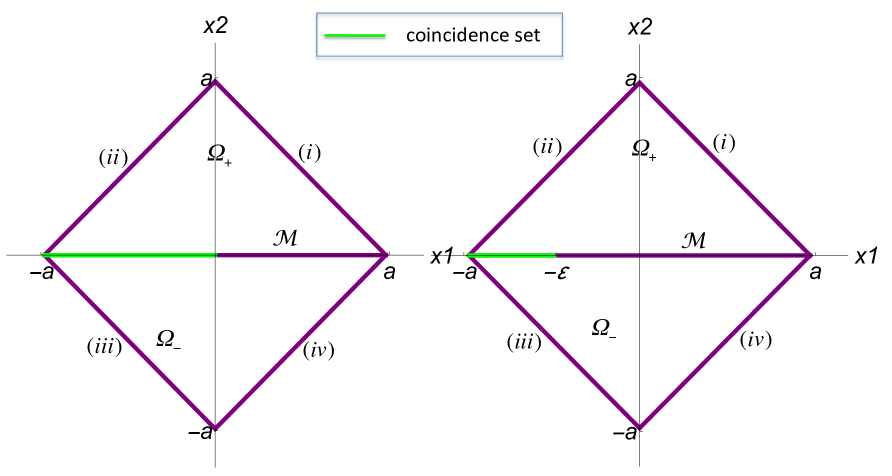
Figure 3: Domains $\Omega_{+}$ and $\Omega_{-}$; coincidence sets for $u$ and $v_{1}$ (left) and for $v_{3,\varepsilon}$ (right)

In this example, $\partial\Omega$ consists of four parts:

$(i)$	$x_{1}+x_{2}-a=0$,		$(iii)$	$-x_{1}-x_{2}-a=0$,
$(ii)$	$-x_{1}+x_{2}-a=0$,		$(iv)$	$x_{1}-x_{2}-a=0$.

Notice that for this example, we can explicitly define the minimizer. It is well known (see [PSU12]) that for all $R>0$

$$u(x_{1},x_{2})=\text{\rm{Re}}\left((x_{1}+i|x_{2}|)^{3/2}\right)$$

is the exact solution of the thin obstacle problem in $B_{R}\subset\mathbb{R}^{2}$ with $\mathcal{M}:=\{x_{2}=0\}$, and $\psi\equiv 0$, and $\varphi=u\big{|}_{\partial B_{R}}$. Here, $B_{R}$ denotes the open ball with center at the origin and radius $R$. It is clear that $\Delta u=0$ in $\Omega_{\pm}$. In addition,

$$u(x_{1},0)=\left\{\begin{aligned} &0,\qquad\text{if}\ x_{1}\leqslant 0,\\ &x_{1}^{3/2},\quad\text{if}\ x_{1}>0\end{aligned}\right.\qquad\text{and}\qquad\left[\frac{\partial u}{\partial\mathbf{n}}\right]=\left\{\begin{aligned} &3\sqrt{-x_{1}},\quad\text{if}\ x_{1}<0,\\ &\ \ 0,\qquad\ \ \text{if}\ x_{1}\geqslant 0.\end{aligned}\right.$$

Setting the boundary condition $\varphi$ on $\partial\Omega$ as the trace of $\text{\rm{Re}}\left((x_{1}+i|x_{2}|)^{3/2}\right)$ and taking $\psi\equiv 0$, we see that the restriction of $u$ to $\Omega$ is the exact solution of the thin obstacle problem in this bounded domain (see Fig. 4 (left)).

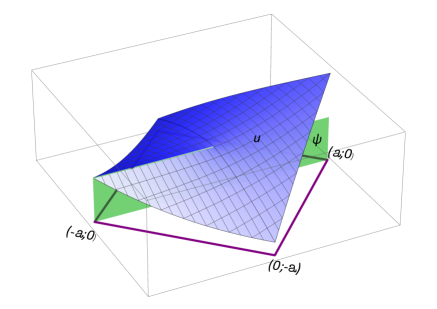
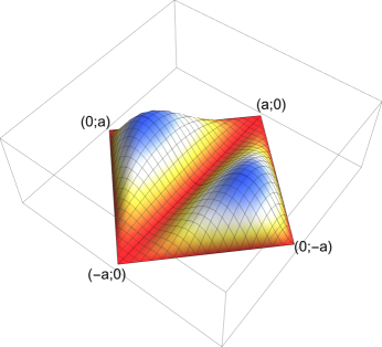
Figure 4: The exact solution $u$ (left) and the function $v_{1}-u$ (right)

In order to verify the performance of our estimates, we select different functions $v$ in $\mathbb{K}$ and compute the distances between $v$ and $u$.

Example 5.1.

First, we define $v=v_{1}$ as follows:

$$v_{1}(x_{1},x_{2}):=u(x_{1},x_{2})+\left\{\begin{aligned} &x_{2}^{2}(x_{2}-x_{1}-a)(x_{2}+x_{1}-a),\quad\text{if}\ x_{2}\geqslant 0,\\ &x_{2}^{2}(x_{2}-x_{1}+a)(x_{2}+x_{1}+a),\quad\text{if}\ x_{2}<0.\end{aligned}\right.$$

It is clear that $v_{1}\in\mathbb{K}$ and $v_{1}\geqslant u$ in $\Omega$ and $v_{1}(x_{1},0)=u(x_{1},0)$. Thus, $v_{1}$ has the same coincidence set as the exact solution $u$ (see Fig. 3 (left) and Fig. 4 (right)).

By direct computations, we find that $\left[\frac{\partial v_{1}}{\partial\mathbf{n}}\right]=\left[\frac{\partial u}{\partial\mathbf{n}}\right]+12ax_{2}^{2}$,

$$\Delta v_{1} =\left\{\begin{aligned} &10x_{2}^{2}-12x_{2}a-2x_{1}^{2}+2a^{2},\quad\text{in}\ \Omega_{+}\\ &10x_{2}^{2}+12x_{2}a-2x_{1}^{2}+2a^{2},\quad\text{in}\ \Omega_{-}\end{aligned}\right.,$$

and the exact error

$$\|\nabla(v_{1}-u)\|_{\Omega}=\frac{4}{3}\sqrt{\frac{2}{35}}a^{4}.$$

Let us set here $q^{*}=\nabla v_{1}$ and $\lambda=\left[\frac{\partial v_{1}}{\partial\mathbf{n}}\right]$. Computing the majorant $\mathfrak{M}\left(v_{1},\nabla v_{1},\left[\frac{\partial v_{1}}{\partial\mathbf{n}}\right],0\right)$, defined by (2.17), we get

$$\mathfrak{M}\left(v_{1},\nabla v_{1},\left[\frac{\partial v_{1}}{\partial\mathbf{n}}\right],0\right) =\|\nabla v_{1}-\nabla v_{1}\|_{\Omega}+\sqrt{2}\left(\int\limits_{-a}^{a}\left[\frac{\partial v_{1}}{\partial\mathbf{n}}\right]v_{1}dx\right)^{1/2}$$ (5.1)

$$+C_{F_{\Omega_{+}}}\|\text{\rm{div}}\,\nabla v_{1}\|_{\Omega_{+}}+C_{F_{\Omega_{-}}}\|\text{\rm{div}}\,\nabla v_{1}\|_{\Omega_{-}}$$

$$+C_{Tr_{\mathcal{M}}}\|\left[\frac{\partial v_{1}}{\partial\mathbf{n}}\right]-\left[\nabla v_{1}\cdot\mathbf{n}\right]\|_{\mathcal{M}}$$

$$=C_{F_{\Omega_{+}}}\|\Delta v_{1}\|_{\Omega_{+}}+C_{F_{\Omega_{-}}}\|\Delta v_{1}\|_{\Omega_{-}}.$$

Remark 5.2.

Here the constants $C_{F_{\Omega_{+}}}$ and $C_{F_{\Omega_{-}}}$ are defined by the quotient type relations

$$\inf\limits_{w\in H^{1}_{0,\pm}(\Omega_{\pm})}\frac{\|\nabla w\|_{\Omega_{\pm}}}{\|w\|_{\Omega_{\pm}}}=\frac{1}{C_{F_{\Omega_{\pm}}}},$$

where $H^{1}_{0,+}(\Omega_{+})$ contains all $H^{1}$-functions vanishing on $(i)$ and $(ii)$ and $H^{1}_{0,-}(\Omega_{-})$ contains all $H^{1}$-functions vanishing on $(iii)$ and $(iv)$. It is easy to show that

$$C_{F_{\Omega_{+}}}=C_{F_{\Omega_{-}}}=\frac{a}{\pi}.$$ (5.2)

Indeed, consider the rotated triangle (see Fig. 5) and the respective eigenvalue problem

$\displaystyle\Delta w+\varkappa w$ $\displaystyle=0\quad\text{in}\quad\Omega_{+},$ $\displaystyle w$ $\displaystyle=0\quad\text{on}\quad\widetilde{x}_{1}=0,$ $\displaystyle w$ $\displaystyle=0\quad\text{on}\quad\widetilde{x}_{2}=0,$ $\displaystyle\frac{\partial w}{\partial\mathbf{n}}$ $\displaystyle=0\quad\text{on}\quad\mathcal{M},$ $\displaystyle\mathcal{M}:=$ $\displaystyle\{\widetilde{x}_{1}+\widetilde{x}_{2}=a\sqrt{2}\},$

Figure 5: Eigenvalue problem

Figure 5 is referred to the eigenvalue problem where the minimal eigenvalue corresponds to the eigenfunction

$$\widetilde{w}=\sin{\left(\frac{\pi}{a\sqrt{2}}\widetilde{x}_{1}\right)}\sin{\left(\frac{\pi}{a\sqrt{2}}\widetilde{x}_{2}\right)}.$$

Direct calculation of $\|\nabla\widetilde{w}\|_{\Omega_{\pm}}$ and $\|\widetilde{w}\|_{\Omega_{\pm}}$ yields (5.2).

Plugging (5.2) into (5.1) yields the equality

$$\mathfrak{M}\left(v_{1},\nabla v_{1},\left[\frac{\partial v_{1}}{\partial\mathbf{n}}\right],0\right)=\frac{16}{3\sqrt{5}\pi}a^{4}.$$

Therefore, the efficiency of the estimate is characterized by the value (efficiency index)

$$1\leqslant\frac{\mathfrak{M}\left(v_{1},\nabla v_{1},\left[\frac{\partial v_{1}}{\partial\mathbf{n}}\right],0\right)}{\|\nabla(v_{1}-u)\|_{\Omega}}=\frac{4}{\pi}\sqrt{\frac{7}{2}}\approx 2.382.$$

It should be pointed out that for $q^{*}=\nabla v_{1}$ and $\lambda=\left[\frac{\partial v_{1}}{\partial\mathbf{n}}\right]$ the assumption (3.7) is fulfilled. Moreover, $\|\left[\frac{\partial v_{1}}{\partial\mathbf{n}}\right]-\left[\nabla v_{1}\cdot\mathbf{n}\right]\|_{\mathcal{M}}=0$. Thus, for any $\alpha\in[0,1]$ we can also compute a version of the majorant $\mathfrak{M}_{3}\left(v_{1},\nabla v_{1},\alpha,\left[\frac{\partial v_{1}}{\partial\mathbf{n}}\right],0\right)$, which is modified in accordance with Remark 3.4. We will denote this modified majorant by $\mathfrak{M}^{\prime}_{3}$. Taking into account (5.2), we get

$$\mathfrak{M}^{\prime}_{3}\left(v_{1},\nabla v_{1},\alpha,\left[\frac{\partial v_{1}}{\partial\mathbf{n}}\right],0\right) =\|\nabla v_{1}-\nabla v_{1}\|_{\Omega}+\sqrt{2}\left(\int\limits_{-a}^{a}\left[\frac{\partial v_{1}}{\partial\mathbf{n}}\right]v_{1}dx\right)^{1/2}$$

$$+\left[C^{2}_{F_{\Omega_{-}}}\|\text{\rm{div}}\,\nabla v_{1}\|^{2}_{\Omega_{-}}+C^{2}_{F_{\Omega_{+}}}\|\text{\rm{div}}\,\nabla v_{1}\|^{2}_{\Omega_{+}}\right]^{1/2}$$

$$=\frac{a}{\pi}\left[\|\Delta v_{1}\|^{2}_{\Omega_{-}}+\|\Delta v_{1}\|^{2}_{\Omega_{+}}\right]^{1/2}=\frac{8\sqrt{2}}{3\sqrt{5}\pi}a^{4}.$$

Hence we have better efficiency index

$$1\leqslant\frac{\mathfrak{M}^{\prime}_{3}\left(v_{1},\nabla v_{1},\alpha,\left[\frac{\partial v_{1}}{\partial\mathbf{n}}\right],0\right)}{\|\nabla(v_{1}-u)\|_{\Omega}}=\frac{2}{\pi}\sqrt{7}\approx 1.684.$$

Finally, we notice that in view of Remark 2.5, the majorant $\mathfrak{M}$ is sharp for $q^{*}=\nabla u$ and $\lambda=\left[\frac{\partial u}{\partial\mathbf{n}}\right]$, i.e.,

$$\frac{\mathfrak{M}(v_{1},\nabla u,\left[\frac{\partial u}{\partial\mathbf{n}}\right],0)}{\|\nabla(v_{1}-u)\|_{\Omega}}=1.$$

Example 5.3.

Consider now another function $v=v_{2}$, where

$$v_{2}(x_{1},x_{2}):=u(x_{1},x_{2})+(x_{1}+x_{2}-a)(x_{2}-x_{1}-a)(x_{1}+x_{2}+a)(x_{2}-x_{1}+a).$$

Obviously, $v_{2}>u$ in $\Omega$. Hence $v_{2}\in\mathbb{K}$ and the respective coincidence set is empty.

Moreover, we have $\Delta v_{2}=8(x_{1}^{2}+x_{2}^{2}-a^{2})$ in $\Omega_{\pm}$, and

$$\left[\frac{\partial{v_{2}}}{\partial\mathbf{n}}\right]=\left[\frac{\partial u}{\partial\mathbf{n}}\right]=\left\{\begin{aligned} &3\sqrt{-x_{1}},\quad\text{if}\ x_{1}<0,\\ &\ \ 0,\qquad\ \ \text{if}\ x_{1}\geqslant 0.\end{aligned}\right.$$ (5.3)

Let $q^{*}=\nabla v_{2}$ and $\lambda=\left[\frac{\partial v_{2}}{\partial\mathbf{n}}\right]$. Then the assumption (3.7) is satisfied. We take into account (5.2), Remark 3.4 and apply use the estimate (3.6), which gives

$$\|\nabla(v_{2}-u)\|_{\Omega}=\frac{16}{3\sqrt{5}}a^{4} \leqslant\sqrt{2}\left(\int\limits_{-a}^{0}3\sqrt{-x_{1}}\,v(x_{1},0)dx_{1}\right)^{1/2}$$

$$+\frac{a}{\pi}\left(\|\Delta v_{2}\|^{2}_{\Omega_{+}}+\|\Delta v_{2}\|^{2}_{\Omega_{-}}\right)^{1/2}.$$

This estimate has the efficiency index

$$1\leq\frac{\mathfrak{M}_{3}\left(v,\nabla v_{2},\left[\frac{\partial v_{2}}{\partial\mathbf{n}}\right],0\right)}{\|\nabla(v_{2}-u)\|_{\Omega}}\leq\frac{\sqrt{22}}{\pi}+\sqrt{\frac{45}{2\cdot 77}}a^{-5/4}\approx 1.493+0.541a^{-5/4},$$

which shows that the upper bound is quite realistic.

In the next example, we study the behavior of error majorants for some sequences of the approximate solutions $(v_{3,\varepsilon})\subset\mathbb{K}$, which converges to the exact solution $u$ as $\varepsilon\to 0$.

Example 5.4.

Let $v=v_{3,\varepsilon}$ be defined as follows:

$$v_{3,\varepsilon}(x_{1},x_{2}):=u(x_{1},x_{2})+\varepsilon^{2}\left\{\begin{aligned} &0,\qquad\qquad\qquad\qquad\qquad\qquad\qquad\text{if}\ (x_{1},x_{2})\in\Omega,\ x_{1}\leqslant-\varepsilon,\\ &\beta(x_{1})(a+x_{1}+x_{2})(a+x_{1}-x_{2}),\quad\text{if}\ (x_{1},x_{2})\in\Omega,\ -\varepsilon<x_{1}\leqslant 0,\\ &\beta(x_{1})(a-x_{1}-x_{2})(a-x_{1}+x_{2}),\quad\text{if}\ (x_{1},x_{2})\in\Omega,\ 0<x_{1}\leqslant a,\end{aligned}\right.$$

where $\varepsilon\in(0;a)$ is an arbitrary small number and $\beta(x_{1})=(a-x_{1})(x_{1}+\varepsilon)^{2}$.

For any $\varepsilon\in(0;a)$ we have $v_{3,\varepsilon}\in\mathbb{K}$, and $v_{3,k}\geqslant u$ in $\Omega$. It is also evident that $\mathcal{M}^{v_{3,\varepsilon}}_{0}\subset\mathcal{M}^{u}_{0}$ (see Fig. 3 (right)); in other words, for any $\varepsilon$ the function $v_{3,\varepsilon}$ has smaller coincidence set that $u$.

First, we set $q^{*}=\nabla u$, $\lambda=\left[\frac{\partial u}{\partial\mathbf{n}}\right]$. Taking into account (5.2) and appyling the estimate (2.17), we obtain by direct calculations the following equalities:

$$\|\nabla(v_{3,\varepsilon}-u)\|_{\Omega} =\frac{2}{15\sqrt{7}}\varepsilon^{2}\mathscr{A}(a,\varepsilon),$$

$$\mathfrak{M}(v_{3,\varepsilon},\nabla u,\left[\frac{\partial u}{\partial\mathbf{n}}\right],0) =\frac{2}{15\sqrt{7}}\varepsilon^{2}\mathscr{A}(a,\varepsilon)+4\sqrt{6}\varepsilon^{11/4}\mathscr{B}(a,\varepsilon),$$

where

$$\mathscr{A}(a,\varepsilon) =(3a^{10}+30a^{9}\varepsilon+135a^{8}\varepsilon^{2}+360a^{7}\varepsilon^{3})^{1/2}+o(\varepsilon^{2}),$$

$$\mathscr{B}(a,\varepsilon) =\left(\frac{a^{3}}{35}-\frac{\varepsilon a^{2}}{105}-\frac{\varepsilon^{2}a}{231}+\frac{\varepsilon^{3}}{429}\right)^{1/2}.$$

Thus, the efficiency index takes the form

$$1\leqslant\frac{\mathfrak{M}(v_{3,\varepsilon},\nabla u,\left[\frac{\partial u}{\partial\mathbf{n}}\right],0)}{\|\nabla(v_{3,\varepsilon}-u)\|_{\Omega}}=1+30\sqrt{42}\varepsilon^{3/4}\frac{\mathscr{B}(a,\varepsilon)}{\mathscr{A}(a,\varepsilon)}.$$ (5.4)

Obviosly, the last term on the right-hand side of (5.4) tends to zero as $\varepsilon\to 0$.

Next, we take $q^{*}=\nabla v_{3,\varepsilon}$ and $\lambda=\left[\frac{\partial v_{3,\varepsilon}}{\partial\mathbf{n}}\right]$. Due to (5.2), (5.3), and the equality $\big{[}\frac{\partial v_{3,\varepsilon}}{\partial\mathbf{n}}\big{]}=\big{[}\frac{\partial u}{\partial\mathbf{n}}\big{]}$, we get

$$\mathfrak{M}\left(v_{3,\varepsilon},\nabla v_{3,\varepsilon},\left[\frac{\partial u}{\partial\mathbf{n}}\right],0\right)=\sqrt{6}\varepsilon\left(\int\limits_{-\varepsilon}^{0}\sqrt{-x_{1}}\beta(x_{1})(a+x_{1})^{2}dx_{1}\right)^{1/2}\\ +\frac{a}{\pi}\left(\|\Delta v_{3,\varepsilon}\|^{2}_{\Omega_{-}}+\|\Delta v_{3,\varepsilon}\|^{2}_{\Omega_{+}}\right)^{1/2}=4\sqrt{6}\varepsilon^{11/4}\mathscr{B}(a,\varepsilon)+\frac{2}{3\pi}\sqrt{\frac{2}{35}}a\varepsilon^{2}\mathscr{C}(a,\varepsilon),$$

where $\mathscr{C}(a,\varepsilon)=(37a^{8}+296a^{7}\varepsilon+2716a^{6}\varepsilon^{2}-1288a^{5}\varepsilon^{3})^{1/2}+o(\varepsilon^{2})$.

In this case, the majorant (2.17) has the efficiency index

$$1\leqslant\frac{\mathfrak{M}(v_{3,\varepsilon},\nabla v_{3,\varepsilon},\left[\frac{\partial v_{3,\varepsilon}}{\partial\mathbf{n}}\right],0)}{\|\nabla(v_{3,\varepsilon}-u)\|_{\Omega}}=30\sqrt{42}\varepsilon^{3/4}\frac{\mathscr{B}(a,\varepsilon)}{\mathscr{A}(a,\varepsilon)}+\frac{a\sqrt{10}}{\pi}\frac{\mathscr{C}(a,\varepsilon)}{\mathscr{A}(a,\varepsilon)}.$$

It is easy to see that if $\varepsilon$ tends to zero then the efficiency index can not exceed $3.54$.

Remark 5.5.

In the above examples, rather simple functions $q^{*}$ and $\lambda$ (constructed directly by means of the function $v$) provide quite realistic bounds of the error. In more complicated examples, such a simple choice might lead to a considerable overestimation of the error. In this case, so defined $q$ and $\lambda$ may be considered as a starting point for the iteration process of majorant minimization that generates a monotonically decreasing sequence of numbers, which are guaranteed upper bounds of the error.

Acknowledgments

D.A. was partly supported by the ”RUDN University Program 5-100” and by the Russian Foundation of Basic Research (RFBR) through the grant 17-01-00678.

S.R. was partly supported by the Russian Foundation of Basic Research (RFBR) through the grant 17-01-00099.

References

- [AC04] I. Athanasopoulos and L. A. Caffarelli. Optimal regularity of lower dimensional obstacle problems. Zap. Nauchn. Sem. S.-Peterburg. Otdel. Mat. Inst. Steklov. (POMI), 310:49–66 [Russian], 2004. English transl. in J. Math. Sci. (N.Y.) 132 (2006), no. 3, 485-498.
- [ACS08] I. Athanasopoulos, L. A. Caffarelli, and S. Salsa. The structure of the free boundary for lower dimensional obstacle problems. Amer. J. Math., 130(2):485–498, 2008.
- [BS00] J. F. Bonnans and A. Shapiro. Perturbation analysis of optimization problems. Springer Series in Operations Research. Springer-Verlag, New York, 2000.
- [Caf79] L.A. Caffarelli. Further regularity for the Signorini problem. Comm. Partial Differential Equations, 4(9):1067–1075, 1979.
- [CSS08] L. A. Caffarelli, S. Salsa, and L. Silvestre. Regularity estimates for the solution and the free boundary of the obstacle problem for the fractional laplacian. Invent. Math., 171(2):425–461, 2008.
- [CT04] R. Cont and P. Tankov. Financial modelling with jump processes. Chapman & Hall/CRC Financial Mathematics Series. Chapman & Hall/CRC, Boca Raton, FL, 2004.
- [DL76] G. Duvaut and J.-L. Lions. Inequalities in mechanics and physics. Springer-Verlag, Berlin, 1976. Translated from the French by C. W. John, Grundlehren der Mathematischen Wissenschaften, 219.
- [DSS16] D. De Silva and O. Savin. Boundary Harnack estimates in slit domains and applications to thin free boundary problems. Rev. Mat. Iberoam., 32(3):891–912, 2016.
- [ET76] I. Ekeland and R. Témam. Convex analysis and variational problems, volume 1 of Studies in Mathematics and its Applications. North-Holland Publishing Co., Amsterdam-Oxford; American Elsevier Publishing Co., Inc., New York, 1976. Translated from the French,.
- [Fic64] G. Fichera. Problemi elastostatici con vincoli unilaterali: il problema di Signorini con ambigue condizioni al contorno. Atti Acad. Naz. Linicei Mem. Cl. Sci. Fis. Mat. Nat. Sez. Ia, 7(8):91–140, 1963-64.
- [Fre75] J. Frehse. Two dimensional variational problems with thin obstacles. Math. Z., 143(3):279–288, 1975.
- [Fre77] J. Frehse. On Signorini’s problem and variational problems with thin obstacles. Ann. Scuola Norm. Sup. Pisa Cl. Sci. (4), 4(2):343–362, 1977.
- [Fri88] A. Friedman. Variational principles and free-boundary problems. Robert E. Krieger Publishing Co. Inc., Malabar, 1988.
- [GP09] N. Garofalo and A. Petrosyan. Some new monotonicity formulas and the singular set in the lower dimensional obstacle problem. Invent. Math., 177(2):415–461, 2009.
- [Gui09] N. Guillen. Optimal regularity for the Signorini problem. Calc. Var. Partial Differential Equations, 36(4):533–546, 2009.
- [IT79] A. D. Ioffe and V. M. Tihomirov. Theory of extremal problems, volume 6 of Studies in Mathematics and its Applications. North-Holland Publishing Co., Amsterdam-New York, 1979.
- [KO88] N. Kikuchi and J. T. Oden. Contact problems in elasticity: a study of variational inequalities and finite element methods, volume 8 of SIAM Studies in Applied Mathematics. Society for Industrial and Applied Mathematics (SIAM), Philadelphia, PA, 1988.
- [KPS15] H. Koch, A. Petrosyan, and W. Shi. Higher regularity of the free boundary in the elliptic Signorini problem. Nonlinear Anal., 126:3–44, 2015.
- [KS00] D. Kinderlehrer and G. Stampacchia. An introduction to variational inequalities and their applications, volume 31 of Classics in Applied Mathematics. Society for Industrial and Applied Mathematics (SIAM), Philadelphia, PA, reprint of the 1980 original edition, 2000.
- [Lew72] H. Lewy. On the coincidence set in variational inequalities. J. Differential Geometry, 6:497–501, 1972. Collection of articles dedicated to S. S. Chern and D. C. Spencer on their sixtieth birthdays.
- [LS67] J.-L. Lions and G. Stampacchia. Variational inequalities. Comm. Pure Appl. Math., 20:493–519, 1967.
- [Mik64] S.G. Mikhlin. Variational methods in mathematical physics. Pergamon, Oxford, 1964.
- [MR16] S. Matculevich and S. Repin. Explicit constants in Poincaré-type inequalities for simplicial domains and application to a posteriori estimates. Comput. Methods Appl. Math., 16(2):277–298, 2016.
- [NR15] A.I. Nazarov and S. I. Repin. Exact constants in Poincaré type inequalities for functions with zero mean boundary traces. Math. Meth. Appl. Sci., 38(15):3195–3207, 2015.
- [PS47] W. Prager and J.L. Synge. Approximation in elasticity based on the concept of function space. Quart. Appl. Math., 5:241–269, 1947.
- [PSU12] A. Petrosyan, H. Shahgholian, and N. Uraltseva. Regularity of free boundaries in obstacle type problems, volume 136 of Graduate Studies in Mathematics. American Mathematical Society, Providence, RI, 2012.
- [PW60] L.E. Payne and H.F. Weinberger. An optimal Poincaré inequality for convex domains. Arch. Ration. Mech. Anal., 5:286–292, 1960.
- [Rep00a] S. I. Repin. Estimates of deviations from exact solutions of elliptic variational inequalities. Zap. Nauchn. Sem. S.-Peterburg. Otdel. Mat. Inst. Steklov. (POMI), 271:188–203 [Russian], 2000. English transl. in J. Math. Sci. (N.Y.) 115, no. 6 (2003), 2811-2819.
- [Rep00b] S. I. Repin. A posteriori error estimation for variational problems with uniformly convex functionals. Math. Comp., 69(230):481–500, 2000.
- [Ric78] D. J. A. Richardson. Variational problems with thin obstacles. ProQuest LLC, Ann Arbor, MI, 1978. Thesis (Ph.D.)–The University of British Columbia (Canada).
- [Rod87] J.-F. Rodrigues. Obstacle problems in mathematical physics, volume 134 of North-Holland Mathematics Studies. North-Holland Publishing Co., Amsterdam, 1987. Notas de Matemática [Mathematical Notes], 114.
- [RV15] S. Repin and J. Valdman. A posteriori error estimates for two-phase obstacle problem. Problems in mathematical analysis, (78):191–200 [Russian], 2015. English transl. in J. Math. Sci. (N.Y.) 207 (2015), no. 2, 324-335.
- [Sil07] L. Silvestre. Regularity of the obstacle problem for a fractional power of the Laplacian operator. Commun. Pure Appl. Math., 60(1):67–112, 2007.
- [SUW04] H. Shahgholian, N. Uraltseva, and G. S. Weiss. Global solutions of an obstacle-problem-like equation with two phases. Monatsh. Math., 142(1-2):27–34, 2004.
- [SUW07] H. Shahgholian, N. Uraltseva, and G. S. Weiss. The two-phase membrane problem—regularity of the free boundaries in higher dimensions. Int. Math. Res. Not. IMRN, (8):1073–7928, 2007.
- [SW06] H. Shagholian and G. S. Weiss. The two-phase membrane problem—an intersection-comparison approach to the regularity at branch points. Adv. Math., 205(2):487–503, 2006.
- [Ura85] N.N. Uraltseva. Hölder continuity of gradients of solutions of parabolic equations with boundary conditions of Signorini type. Dokl. Akad. Nauk SSSR, 280(3):563–565, 1985.
- [Ura01] N. N. Uraltseva. Two-phase obstacle problem. J. Math. Sci. (New York), 106(3):3073–3077, 2001. Function theory and phase transitions.
- [Wei01] G. S. Weiss. An obstacle-problem-like equation with two phases: pointwise regularity of the solution and an estimate of the Hausdorff dimension of the free boundary. Interfaces Free Bound., 3(2):121–128, 2001.