NuSTAR and Swift observations of the ultraluminous X-ray source IC 342 X-1 in 2016: witnessing spectral evolution

Abstract

We report on an X-ray observing campaign of the ultraluminous X-ray source IC 342 X-1 with NuSTAR and Swift in 2016 October, in which we captured the very moment when the source showed spectral variation. The Swift/XRT spectrum obtained in October 9–11 has a power-law shape and is consistent with those observed in the coordinated XMM-Newton and NuSTAR observations in 2012. In October 16–17, when the 3–10 keV flux became $\approx$4 times higher, we performed simultaneous NuSTAR and Swift observations. In this epoch, the source showed a more round-shaped spectrum like that seen with ASCA 23 years ago. Thanks to the wide energy coverage and high sensitivity of NuSTAR, we obtained hard X-ray data covering up to $\sim$30 keV for the first time during the high luminosity state of IC 342 X-1. The observed spectrum has a broader profile than the multi-color disk blackbody model. The X-ray flux decreased again in the last several hours of the NuSTAR observation, when the spectral shape approached those seen in 2012 and 2016 October 9–11. The spectra obtained in our observations and in 2012 can be commonly described with disk emission and its Comptonization in cool ($T_{\rm e}\approx 4$ keV), optically-thick ($\tau\approx 5$) plasma. The spectral turnover seen at around 5–10 keV shifts to higher energies as the X-ray luminosity decreases. This behavior is consistent with that predicted from recent numerical simulations of super-Eddington accretion flows with Compton-thick outflows. We suggest that the spectral evolution observed in IC 342 X-1 can be explained by a smooth change in mass accretion rate.

I. Introduction

Table 1Log of Swift and NuSTAR observations

ObsID	Start time (UT)	End time (UT)	Net exposure (ks)
NuSTAR			FPMA	FPMB
90201039002	2016 Oct. 16 02:11:08	2016 Oct. 17 02:51:08	49.1	49.0
Swift			XRT
00031987018	2016 Oct. 09 03:42:38	2016 Oct. 09 05:34:52	0.94
00080321019	2016 Oct. 10 03:34:04	2016 Oct. 10 05:25:54	0.94
00080321020	2016 Oct. 11 03:31:38	2016 Oct. 11 05:20:55	0.94
00080321001	2016 Oct. 16 06:23:00	2016 Oct. 16 06:38:53	0.94
00080321002	2016 Oct. 16 10:54:26	2016 Oct. 16 11:10:54	0.96
00080321003	2016 Oct. 16 14:05:26	2016 Oct. 16 14:18:53	0.78
00080321004	2016 Oct. 16 18:51:30	2016 Oct. 16 19:08:53	1.0
00080321005	2016 Oct. 16 22:03:30	2016 Oct. 16 22:20:54	1.0
00080321006	2016 Oct. 17 01:18:33	2016 Oct. 17 01:34:53	0.96

Ultraluminous X-ray sources (ULX: Makishima et al., 2000), found in off-nuclear regions of nearby galaxies, have luminosities exceeding the Eddington limit for stellar-mass black holes: $\sim 10^{39}$ erg s^-1 (Fabbiano, 1989). The mass of the compact object and the mass accretion rate of ULXs have been controversial. There have been two major ideas present: (1) an intermediate mass ($\gtrsim 100M_{\sun}$) black hole accreting at sub-Eddington rates (e.g., Colbert & Mushotzky, 1999; Makishima et al., 2000; Miller et al., 2003) and (2) a smaller mass black hole: a stellar-mass (up to a few ten $M_{\sun}$) black hole accreting at super-Eddington rates (e.g., Fabrika & Mescheryakov, 2001; King et al., 2001; Watarai et al., 2001; Ebisawa et al., 2003; Poutanen et al., 2007) or a black hole with several ten $M_{\sun}$ produced from low metallicity stars (e.g., Mapelli et al., 2009; Belczynski et al., 2010) accreting at or above Eddington rates. If the former is the case, they could be the long-sought missing link between stellar-mass black holes and supermassive black holes in the center of galaxies. If the latter is the case, they would be the best laboratory to study super-Eddington accretion. In any case, ULXs are important objects in many aspects, including physics of black hole accretion, and formation/growth of binary systems and black holes themselves.

While extremely luminous ULXs are suggested to harbor an intermediate mass black hole accreting at sub-Eddington rates (Farrell et al., 2009; Sutton et al., 2012), the dominant population, with luminosities just above $10^{39}$ erg s^-1 up to $\sim 10^{40}$ erg s^-1 (Swartz et al., 2011; Walton et al., 2011), encompasses the most promising candidates of stellar-mass, super-Eddington accretors. Signs of massive outflows, predicted by numerical simulations of super-Eddington accretion flows (Ohsuga et al., 2005; Ohsuga & Mineshige, 2011), have been found directly and indirectly. Middleton et al. (2014) suggested that the residuals seen in many ULX spectra can be explained by absorption structures of ultrafast disk winds with a velocity of $\sim 0.1c$. Indeed, absorption features of such massive winds have now been discovered at $\sim$1 keV in the ULX NGC 1313 X-1 (Pinto et al., 2015), although the statistical significance is still not very high. Moreover, Walton et al. (2016) have recently detected a weak Fe K$\alpha$ absorption line at 8.8 keV in the same object and estimated the outflow velocity of $\sim 0.2$c, which is consistent with that obtained in Pinto et al. (2015). Deep optical spectroscopy of several ULXs also suggests the existence of disk winds (Fabrika et al., 2015). These results support that super-Eddington accretors are actually present in the ULXs. In addition, X-ray pulsars have recently been detected in a few ULXs (Bachetti et al., 2014; Israel et al., 2016; Fürst et al., 2016; Israel et al., 2017), and at least one of them shows a typical X-ray spectrum of the known ULXs. This may suggest that, although only a small number of the detections have been present so far, neutron star binaries at super-Eddington luminosities constitute a substantial population of ULXs.

To understand the physical origin of the strong radiation from ULXs, Galactic black hole X-ray binaries (BHXBs) can be used for comparison as a template of accreting stellar-mass black holes below Eddington luminosity. Thanks to their proximity, BHXBs are very bright in their outbursts and have provided high-quality broad-band X-ray data. They show several distinct spectra at different luminosities (see McClintock & Remillard, 2006; Done et al., 2007, for reviews). The two states that are most often seen are the low/hard state, with a hard power-law spectra with an exponential cutoff at $\sim 100$ keV, and the high/soft state, in which a soft X-ray emission from the standard accretion disks (Shakura & Sunyaev, 1973) dominates the spectrum.

Spectral variability of ULXs has been studied by compiling data from snapshot observations (e.g., Pintore & Zampieri, 2012; Pintore et al., 2014; Walton et al., 2014). The results show that ULXs exhibit a variety of X-ray spectra (Sutton et al., 2013) but have some distinct characteristics in their spectral profiles compared with those seen in Galactic BHXBs. They usually have a spectral turnover at energies from a few keV to just above 10 keV (e.g., Gladstone et al., 2009), much lower than that in the low/hard state in Galactic BHXBs. For some ULXs, the inner disk temperature ($T_{\rm in}$) estimated from their spectra anti-correlates with the luminosity ($L$), instead of the $L\propto T_{\rm in}^{4}$ relation, which usually holds in the high/soft state of BHXBs (Feng & Kaaret 2009; Kajava & Poutanen 2009; but see Miller et al. 2013). These differences may suggest that ULXs have different properties of accretion flows from those of Galactic BHXBs, although more X-ray observations, in particular during state transitions, would be needed for a deeper understanding of the origin of such variability.

In 2016 October, we carried out an X-ray observing campaign of the ULX IC 342 X-1 with Nuclear Spectroscopic Telescope Array (NuSTAR; Harrison et al., 2013) and Swift (Gehrels et al., 2004), in which we successfully monitored its spectral evolution. IC 342 X-1 has been observed quite intensively in the X-ray band. Comparing ASCA data taken in 1993 and 2000, Kubota et al. (2001) reported a transition between “the disk dominant state” at a high luminosity and “the power-law spectral state” at a low luminosity. Spectral variation was observed in the former state, which was interpreted as a change in the inner disk radius and temperature (Mizuno et al., 2001). A similar round-shaped spectrum was detected with Chandra as well (Marlowe et al., 2014). Yoshida et al. (2013) found two distinct power-law spectral states at different luminosities, which showed a spectral turnover at different energies. The lower-luminosity power-law state was studied more deeply with high-quality broad-band X-ray data covering up to $\approx 30$ keV with coordinated XMM-Newton and NuSTAR observations in 2012 (Rana et al., 2015), which confirmed the presence of the spectral turnover at $\approx 10$ keV.

In this paper, we report the results of the observations in 2016 October. Section II describes the details of the observations and the data reduction. Section III presents spectral analysis that we performed. In Section IV we discuss possible physical interpretations of the results and the mass of the compact object in IC 342 X-1. In all sections, errors represent the 90% confidence range for a single parameter, unless otherwise stated. We used HEASOFT version 6.19 for data reduction, and XSPEC version 12.9.0n for spectral analysis. Throughout the article, we refer to the table given by Wilms et al. (2000) as the solar abundances. We assumed the distance to the galaxy IC 342 as 3.93 Mpc (Tikhonov & Galazutdinova, 2010).

II. Observations and Data Reduction

We performed NuSTAR time-of-opportunity (ToO) observation of IC 342 X-1 in 2016 October 16–17 with a net exposure of $\approx$50 ksec. We also carried out Swift ToO observations 9 times in 2016 October, each of which have a net exposure of $\sim$1 ks. Six of them were performed in $\approx$2-hour intervals during the NuSTAR observation and the rest were on October 9, 10, and 11. A log of the observations is given in Table 1.

The NuSTAR data were processed by using the tools nupipeline included in the NuSTAR Data Analysis Software (nustardas) version 1.6.0 with the calibration database (CALDB) version 20160922. The source and background extraction regions were defined as circular regions with a radius of 50” centered on the target position (which is the same as Rana et al. 2015) and with a radius of 80” in a nearby source free region on the same detector, respectively. NuSTAR light curves for each of focal plane modules (FPMA and FPMB) were produced through nuproducts with standard settings for point sources described in the NuSTAR analysis guide. The Swift/XRT data were reprocessed with Swift CALDB version 20160706 through the pipeline tool xrtpipeline. The source events were extracted from a circular region centered on the source position with a radius of 30” and background events were from a circle with a radius of 4.8’ in a nearby source-free field on the same detector.

Figure 1 shows the Swift/XRT light curve of IC 342 X-1 in the 0.3–10 keV band for the past $\approx$6 years. This was made with the online data analysis tools provided by the UK Swift Science Data Centre at the University of Leicester. The count rate varied by a factor of $\approx$4. The source was in the lowest flux state on 2016 October 9, 10, and 11, whereas the flux reached the maximum level in our NuSTAR observation performed about 1 week after. Figure 2 presents the background-subtracted NuSTAR light curves and the hardness ratio. The source kept a fairly constant X-ray flux during the first two thirds of the entire period in the NuSTAR observation, and afterwards it gradually become fainter and harder.

To study the spectral evolution, we split the NuSTAR observation into two phases based on the count rate and hardness ratio (see Fig 2): MJD 57677.094–57677.847 (hereafter Phase 1) and MJD 57677.847–57678.347 (Phase 2). We created the time-averaged NuSTAR and Swift/XRT spectra for each of them.

NuSTAR spectra and response files for the individual phases were produced with nuproducts. We combined all the Swift/XRT data in the same phase. Four of six datasets taken in October 16 (ObsID 00080321001, 00080321002, 00080321003, and 00080321004) and two of them taken in October 16–17 (ObsID 00080321005 and 00080321006) were co-added to produce the time-averaged XRT spectra for Phase 1 and Phase 2, respectively. The redistribution matrix file (RMF) swxpc0to12s6_20130101v014.rmf was used for the XRT spectra. The auxiliary response file (ARF) for each phase was generated via xrtmkarf by using a combined exposure map created from the data of all ObsIDs for the same phase. The time-averaged XRT spectrum for October 9–11 and its ARF were also made in the same manner by combining the three observations in that period.

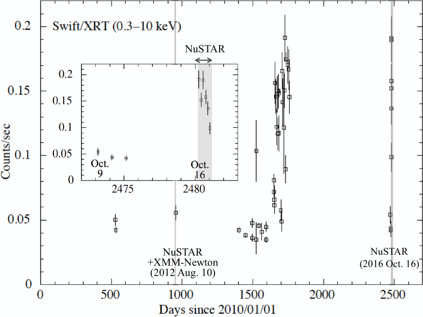
Figure 1.— Swift/XRT 3–10 keV light curve of IC 342 X-1 with one point per observation. The NuSTAR observation performed in 2016 October 16–17 and the coordinated XMM-Newton$+$NuSTAR observation on 2012 August 10 are also indicated as grey shaded regions. The inset is an enlarged view focusing on the period of our observing campaign in 2016.

Figure 2.— NuSTAR/FPMA light curves of IC 342 X-1 in the 3–10 keV (top) and 10–20 keV bands (middle) and the hardness ratios (bottom). The observation period is divided into two phases: MJD 57677.094–57677.847 (Phase 1) and MJD 57677.847–57678.347 (Phase 2), which are used to produce X-ray spectra separately for different hardness ratios.

For comparison, we also reduced the ASCA data taken in 1993, and the simulnatenous XMM-Newton and NuSTAR data in 2012 August 10 (ObsID$=$0693850601 and 30002032003, respectively; see Rana et al. 2015 for more details of the observations) and created the time-averaged broad-band X-ray spectra. The ASCA data were reduced in the same manner as Okada et al. (1998) by using the archival data and the ASCA CALDB downloaded from the HEASARC online CALDB page on 2016 December 10. For the XMM-Newton data, we utilized the Science Analysis System (SAS) version 15.0.0 and the latest Current Calibration File (CCF) as of 2016 October 23 to reprocess them and produce the spectrum. We excluded high background intervals following the XMM-Newton ABC Guide and selected events with FLAG==0 && PATTERN <= 4 for EPIC-pn and with FLAG==0 && PATTERN <= 12 for the two EPIC-MOS cameras. The source and background events were extracted from a circular region with a radius of 30” centered on the source position and with a radius of 60” in a nearby source-free region on the same detector, respectively. The RMF and ARF were generated with the SAS tools rmfgen, and arfgen, respectively. The NuSTAR data were reduced in the same manner with the same software as the 2016 data.

The NuSTAR FPMA and FPMB spectra were combined by using addascaspec to improve statistics and used throughout the following spectral modelling. We have confirmed that the results remain unchanged within the 90% confidence ranges if the two spectra are analyzed separately. Considering the low statistics and relatively large uncertainty of the Swift/XRT data, we fixed the cross normalizations between the Swift/XRT and NuSTAR data for the two phases at $1:1$. We confirmed that their normalizations for Phase 1 and for Phase 2 were consistent within uncertainties at $\lesssim 10$% and $\lesssim 20$% levels, respectively. For 2012 data, the normalizations of the XMM-Newton/EPIC-pn, EPIC-MOS1, and EPIC-MOS2 spectra were found to be consistent with each other at $\sim 3$% levels, while a $\sim 10$% difference was detected between those of the XMM-Newton and NuSTAR spectra. Thus we set the cross normalization among the cameras of XMM-Newton as $1:1:1$ and varied that between the XMM-Newton and NuSTAR.

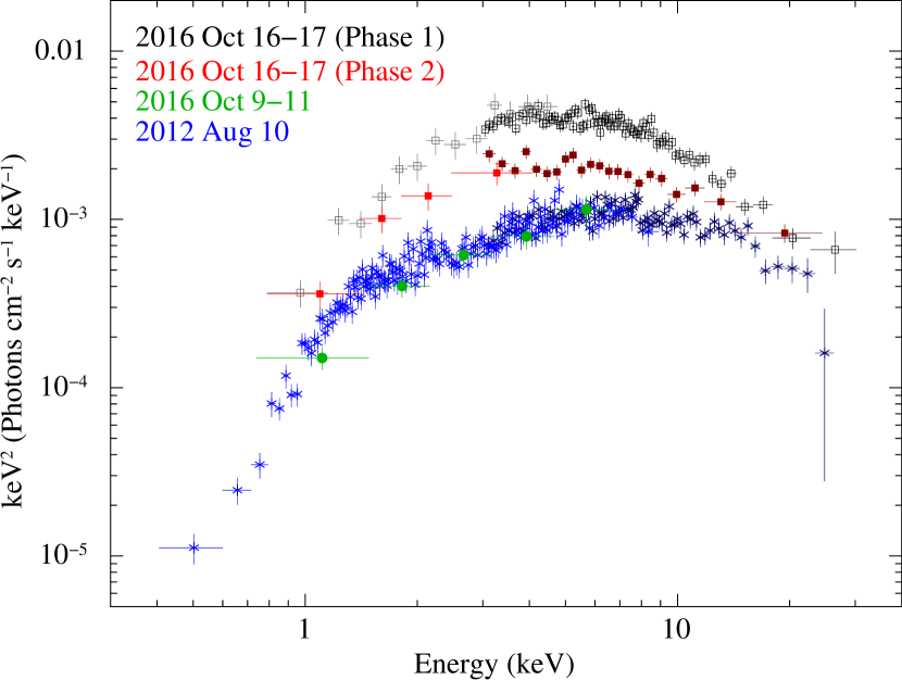
Figure 3.— Time-averaged spectra of IC 342 X-1 in different epochs. Black open squares and red filled squares present the simultaneous Swift/XRT and NuSTAR spectra in the two phases defined in Figure 2. The Swift/XRT spectrum in 2016 October 9–11 is plotted in green (filled circle), and the XMM-Newton$+$NuSTAR data taken in 2012 August 10 are shown in blue (cross). The darker colors indicate the NuSTAR data and the brighter colors correspond to the Swift or XMM-Newton data. Only EPIC-MOS1 data are shown for the XMM-Newton spectrum. FPMA and FPMB data are combined in all NuSTAR spectra.

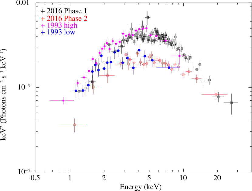
Figure 4.— Comparison of the spectra in Phase 1 (black open squares) and Phase 2 (red open circles), and the ASCA/GIS2 spectra obtained in 1993 during the high-flux periods (pink filled squares) and the low-flux periods (blue filled circles) defined in Mizuno et al. (2001).

III. Spectral Analysis and Results

III.1. Long-term Spectral Variation

In Figure 3, we present the time-averaged NuSTAR and Swift/XRT spectra on different occasions in 2016 October. For comparison, we also plot the simultaneous NuSTAR$+$XMM-Newton spectra obtained on 2012 August 10. The spectrum in 2016 October 9–11 is fully consistent with that obtained in 2012, suggesting that the source was in the same state during the two epochs.

About 1 week after the Swift/XRT observations, the source increased its luminosity and changed the profile of the continuum spectrum. In Phase 1, it marked the highest 3–20 keV flux in Figure 3. It showed a more round shaped spectrum, which start bending at a somewhat lower energy than the spectrum in 2012. The Phase-1 spectrum below $\approx$10 keV looks like that in the “soft state” observed with ASCA in 1993 (Kubota et al., 2001; Mizuno et al., 2001), which was well reproduced with a single multi-color disk blackbody model (MCD model; Mitsuda et al., 1984). In Figure 4, we compare the ASCA spectra and the NuSTAR$+$Swift spectra. We find that the Phase-1 spectrum has a similar continuum profile to that obtained during the high-flux periods (Mizuno et al., 2001) in the ASCA observation.

As the X-ray flux decreased from Phase 1 to Phase 2, the spectral shape became consistent with that in the low-flux periods of the ASCA observation in 1993 (see Fig. 4) and got closer to what was seen in 2012. The Phase-2 spectrum has a spectral turnover at a similar energy to the Phase-1 spectrum, but below that energy, it appears to have a somewhat flatter profile in the $\nu F\nu$ form, like the 2012 data (Fig. 3). In the following sections, we attempt to assess the differences/similarities in continuum profile among the two phases and the 2012 epoch more quantitatively.

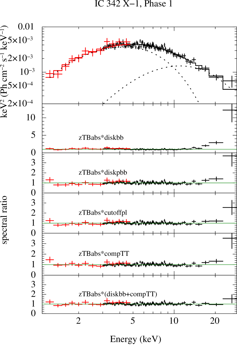
Figure 5.— Results of spectral fit for Phase 1 with various models. Swift and NuSTAR data are shown in red and black, respectively. The top panel presents the Phase-1 spectrum and the best-fit zTBabs*(diskbb+compTT) model. The dotted lines show the contributions of the diskbb component (with a lower peak energy) and the compTT component (higher peak energy). The rest panels plot the data-to-model ratios for the zTBabs*diskbb, zTBabs*diskpbb, zTBabs*cutoffpl, zTBabs*compTT, and zTBabs*(diskbb+compTT) models, from top to bottom.

Table 2Best-fit parameters of various spectral models for the NuSTAR$+$Swift data in Phase 1 and Phase 2 and the NuSTAR$+$XMM-Newton data in 2012

Parameter	Unit	Phase 1	Phase2	2012 August 10
Model: zTBabs*diskbb
$N_{\rm H}$	$10^{22}$ cm-2	$0.02^{+0.09}_{-0.02~{}{\rm(pegged)}}$	0.0 (fixed)	$2^{+9}_{-2~{}{\rm(pegged)}}\times 10^{-3}$
$kT_{\rm in}$	keV	$2.35\pm 0.05$	$2.51^{+0.13}_{-0.12}$	$2.40\pm 0.05$
$N_{\rm diskbb}$		$(2.0\pm 0.2)\times 10^{-2}$	$(8.4\pm 0.2)\times 10^{-3}$	$5.1^{+0.5}_{-0.4}\times 10^{-3}$
$\chi^{2}/$d.o.f.		$176/94=1.87$	$70/24=2.91$	$1965/716=2.74$
Flux	$10^{-11}$ erg cm-2 s-1	$1.3$	$0.71$	$0.37$
Luminosity	$10^{40}$ erg s-2	$2.4$	$1.3$	$0.68$
Model: zTBabs*diskpbb
$N_{\rm H}$	$10^{22}$ cm-2	$0.8^{+0.3}_{-0.2}$	$0.8$ (fixed)	$0.27\pm 0.02$
$kT_{\rm in}$	keV	$3.1\pm 0.2$	$4.0^{+0.4}_{-0.3}$	$4.6^{+0.3}_{-0.2}$
$p$		$0.52^{+0.02}_{-0.02~{}{\rm(pegged)}}$	$0.50^{+0.01}_{-0.00~{}{\rm(pegged)}}$	$0.544\pm 0.005$
$N_{\rm diskbb}$		$2.1^{+1.2}_{-0.7}\times 10^{-3}$	$3.5^{+1.9}_{-1.2}\times 10^{-4}$	$1.4^{+0.4}_{-0.3}\times 10^{-4}$
$\chi^{2}/$d.o.f.		$100/93=1.08$	$20/23=0.86$	$846/715=1.18$
Flux	$10^{-11}$ erg cm-2 s-1	$2.4$	$1.4$	$0.55$
Luminosity	$10^{40}$ erg s-2	$4.3$	$2.6$	$1.0$
Model: zTBabs*cutoffpl
$N_{\rm H}$	$10^{22}$ cm-2	$0.6\pm 0.2$	0.6 (fixed)	$0.24\pm 0.02$
$\Gamma$		$1.15\pm 0.20$	$1.65^{+0.19}_{-0.21}$	$1.46\pm 0.05$
$E_{\rm cut}$	keV	$4.9^{+0.7}_{-0.6}$	$9.0^{+3.3}_{-2.1}$	$11.8^{+1.4}_{-1.2}$
$N_{\rm cutoffpl}$	photon keV-1 cm-2 s-1	$2.9^{+0.6}_{-0.5}\times 10^{-3}$	$(2.1\pm 0.4)\times 10^{-3}$	$6.7^{+0.4}_{-0.3}\times 10^{-4}$
$\chi^{2}/$d.o.f.		$88/93=0.95$	$17/23=0.74$	$883/715=1.24$
Flux	$10^{-11}$ erg cm-2 s-1	$1.8$	$1.2$	$0.55$
Luminosity	$10^{40}$ erg s-2	$3.4$	$2.3$	$1.0$
Model: zTBabs*compTT
$N_{\rm H}$	$10^{22}$ cm-2	$0.0^{+0.1}_{-0.0~{}{\rm(pegged)}}$	0 (fixed)	$0.22\pm 0.03$
$kT_{\rm 0}$	keV	$0.63\pm 0.06$	$0.54^{+0.08}_{-0.07}$	$0.20\pm 0.02$
$kT_{\rm e}$	keV	$2.8^{+0.3}_{-0.2}$	$3.8^{+1.4}_{-0.7}$	$3.2^{+0.2}_{-0.1}$
$\tau$		$5.4\pm 0.6$	$4.4^{+1.1}_{-0.9}$	$6.4\pm 0.3$
$N_{\rm compTT}$		$1.1^{+0.1}_{-0.2}\times 10^{-3}$	$(4.8\pm 0.1)\times 10^{-4}$	$4.7^{+0.5}_{-0.4}\times 10^{-4}$
$\chi^{2}/$d.o.f.		$97/92=1.05$	$17/22=0.77$	$758/714=1.06$
Flux	$10^{-11}$ erg cm-2 s-1	$1.3$	$0.81$	$0.48$
Luminosity	$10^{40}$ erg s-2	$2.4$	$1.5$	$0.89$
Model: zTBabs*(diskbb+compTT)
$N_{\rm H}$	$10^{22}$ cm-2	$0.2\pm 0.1$	0.2 (fixed)	$0.56\pm 0.08$
$kT_{\rm in}$	keV	$1.75^{+0.09}_{-0.02}$	$0.6^{+1.2}_{-0.5}$	$0.20\pm 0.02$
$N_{\rm bb}$		$6^{+9}_{-2}\times 10^{-2}$	$0.5^{+0.5}_{-0.5~{}{\rm(pegged)}}$	$1.5^{+1.7}_{-0.8}\times 10^{2}$
$kT_{\rm e}$	keV	$>3.0~{}(3.9)$	$3.7^{+1.4}_{-1.1}$	$3.2\pm 0.2$
$\tau$		$>0.08~{}(5.8)$	$>3.4~{}(4.5)$	$6.3^{+0.4}_{-0.3}$
$N_{\rm compTT}$		$(1.0^{+9.9}_{-0.8})\times 10^{-4}$	$(4\pm 3)\times 10^{-4}$	$(4.9\pm 0.5)\times 10^{-4}$
$\chi^{2}/$d.o.f.		$81/91=0.89$	$17/21=0.81$	$709/713=0.995$
Flux	$10^{-11}$ erg cm-2 s-1	$1.5$	$0.89$	$0.82$
Luminosity	$10^{40}$ erg s-2	$2.7$	$1.6$	$1.5$

Note. — All the fluxes and luminosities listed above are unabsorbed values estimated in the 0.3–30 keV band. In all models, we included an additional TBabs component with $N_{\rm H}=3.0\times 10^{21}$ cm^-2 as the Galactic absorption, which is omitted in the table.

III.2. Modelling the Phase-1 Spectrum

To begin with, we focus on the Phase-1 data, which have much better statistics than the Phase-2 data. We perform spectral fitting using several models frequently adopted in previous studies of ULXs, and thereby describe the continuum profile in the high luminosity state of IC 342 X-1. The resultant parameters for each model are summarized in Table 2 and the residuals of the fit are presented in Figure 5. In all models, we consider the Galactic absorption with an equivalent hydrogen column density of $N_{\rm H}=3.0\times 10^{21}$ cm^-2 (which is estimated from the H_I all-sky map by Kalberla et al. (2005) via the ftool command nh), in addition to the neutral absorption in the binary system and the host galaxy with a redshift of $z=0.00095$. We use TBabs and zTBabs for the Galactic and local absorptions, respectively, and vary $N_{\rm H}$ of the latter as a free parameter.

We first investigate if a single MCD model can reproduce the observed spectrum as in the case of the ASCA data (Kubota et al., 2001). We find that this model does not produce an acceptable fit ($\chi^{2}/{\rm d.o.f.}=176/94$). As shown in Figure 5, there remains significant deviation between the data and the model at the highest energies, suggesting that the observed continuum profile is broader than the MCD spectrum.

A wider disk spectrum is realized in the case of the so-called “slim disk”, which is believed to form at super-Eddington accretion rates (Abramowicz et al., 1988). A slim disk has a smaller index $p$ of the radial dependence of the temperature than that for the standard accretion disks and thus produces a more broadened spectral profile. We replace the MCD component with diskpbb (Mineshige et al., 1994), where $p$ can vary, and fit the Phase-1 spectrum. The quality of fit is significantly improved from the result of the MCD model and become an acceptable level ($\chi^{2}/{\rm d.o.f.}=100/93$). Although the structures of residuals above 10 keV in Figure 5 are quite evident, it is much less so for those below $\approx 2$ keV.

The spectral turnover seen at $\sim 10$ keV in ULX spectra are often explained by an optically-thick thermal Comptonization in the corona above the accretion disks or in strong outflows suggested to be driven from supercritical accretion flows (e.g., Ohsuga et al., 2005). We next investigate the possibility that such a Comptonized spectrum can reproduce the data. We apply two different models individually: a cutoff power-law (cutoffpl) model as an approximation of a Comptonized spectrum, and the compTT model (Titarchuk, 1994) as a more physical model. The latter model produces thermal Comptonized spectrum employing the Wien profile as the energy distribution of the seed photons. We leave the optical depth and the seed photon temperature as free parameters. Both models yield acceptable fits, but the structure of residuals similar to the diskpbb model remain both in the cutoffpl and compTT models (see Fig. 5).

The single compTT model assumes that the inner disk region emitting X-rays is fully obscured by the surrounding corona or outflows. To account for the possibility that the direct emission from the disk is visible outside the Comptonizing gas, we add a diskbb component and link its inner disk temperature ($T_{\rm in}$) and the seed-photon temperature ($T_{\rm 0}$) of the compTT component. We find that this model can better reproduce the overall profile of the Phase-1 spectrum than the single compTT model. The $\chi^{2}$ value is reduced, and the discrepancies between the data and model are mitigated.

III.3. Modelling the spectra in Phase 2 and in 2012

Using the models employed above, we next analyze the Phase 2 spectrum to characterize its continuum shape. For comparison, we also apply the same models to the 2012 spectrum, which is one of the highest quality data with the widest energy coverage among the low-luminosity state spectra of IC 342 X-1. The resultant parameters for each model in each epoch are listed in Table 2. For Phase 2, the parameters of diskbb, the seed temperature of comptt, and $N_{\rm H}$ are found to degenerate strongly due to poor statistics of the XRT data below $\approx 3$ keV. We thus fix $N_{\rm H}$ at the best-fit value for Phase 1 obtained with the same model.

We find that the Phase 2 and 2012 spectra, as well as that of Phase 1, cannot be reproduced with the single diskbb model. Comparing the resultant parameters of the phenomenological cutoffpl model, a remarkable difference can be seen between Phase 1 and Phase 2: the photon index ($\Gamma$) and the cutoff energy ($E_{\rm cut}$) are significantly larger in the latter than the former. We note that these differences are significant even if we vary $N_{\rm H}$ in Phase 2. The values of $\Gamma$ and $E_{\rm cut}$ in Phase 2 are consistent with those estimated for the 2012 spectrum. This suggests that the spectral profile became closer to that of the 2012 spectrum as the X-ray flux decreased from Phase 1 to Phase 2. In the single compTT and diskbb+compTT models, however, we do not detect any significant differences in the values of $T_{\rm e}$ and $\tau$.

Figure 6.— Absorption corrected best-fit diskbb+compTTm models and data in 2012, Phase 1, and Phase 2 from top to bottom. The contributions of the diskbb and compTTm components are plotted in red dotted and blue dashed lines, respectively. Only the EPIC-MOS1 and NuSTAR data are shown in the top panel.

III.4. Comparison of the spectra in 2016 and 2012 using a modified compTT model

Table 3Best-fit parameters of diskbb+compTTm models for the 2012 data and the 2016 data in Phase 1 and Phase 2

Parameter	Unit	2012	2016, Phase 1	2016, Phase 2
$N_{\rm H}$	$10^{22}$ cm-2	$0.37^{+0.05}_{-0.04}$	$0.4^{+0.4}_{-0.4~{}{\rm(pegged)}}$	$0.4$ (fixed)
$kT_{\rm in}$	keV	$0.40\pm 0.05$	$0.40\pm 0.07$	$0.25^{+0.11}_{-0.7}$
$N_{\rm bb}$		$5^{+5}_{-2}$	$9^{+18}_{-7}$	$32^{+80}_{-32~{}{\rm(pegged)}}$
$kT_{\rm 0}/kT_{\rm in}$		$2.0\pm 0.1$	$2.0$ (fixed)	$2.0$ (fixed)
$kT_{\rm e}$	keV	$3.7^{+0.6}_{-0.4}$	$3.3^{+1.3}_{-0.5}$	$3.9^{+2.0}_{-0.7}$
$\tau$	keV	$5.1^{+0.7}_{-0.8}$	$4.2^{+1.0}_{-1.4}$	$4.2^{+1.0}_{-1.3}$
$N_{\rm compTT}$		$(1.6\pm 0.3)\times 10^{-4}$	$(8\pm 3)\times 10^{-4}$	$(5\pm 3)\times 10^{-4}$
$\chi^{2}/$d.o.f.		$699/712=0.98$	$89/91=0.97$	$17/21=0.79$
Flux	$10^{-11}$ erg cm-2 s-1	$0.57$	$1.7$	$1.1$
Luminosity	$10^{40}$ erg s-2	$1.0$	$3.1$	$2.0$

Note. — The flux and luminositys listed above are unabsorbed values estimated in the 0.3–30 keV band. In all models, we included an additional TBabs component with $N_{\rm H}=3.0\times 10^{21}$ cm^-2 as the Galactic absorption, which is omitted in the table.

In the previous sections, we assumed that the inner disk temperature of the diskbb component is the same as the temperature of seed photons for the compTT component. However, the seed temperature could be higher than the inner temperature determined from the direct MCD component, if the inner disk region is covered by optically-thick Comptonizing cloud and the pure MCD emission is only visible outside it. To investigate if the two temperatures can differ, we attempt to model the spectra in 2012 and 2016 varying $T_{0}$ and $T_{\rm in}$ independently. For this purpose, we modified the code of compTT so that $T_{0}$ is internally calculated from the two input parameters, $T_{\rm in}$ and $T_{\rm 0}/T_{\rm in}$. This model, that hereafter we call compTTm, enable to vary $T_{\rm 0}$ and $T_{\rm in}$ keeping the condition $T_{\rm in}<T_{\rm 0}$.

We first fit the 2012 spectrum with the diskbb+compTTm model, where we link $T_{\rm in}$ of the two components and set the lower limit of $T_{\rm 0}/T_{\rm in}$ to be 1. The model gives an acceptable fit with $T_{\rm 0}/T_{\rm in}=2.0\pm 0.1$. The resultant parameters are listed in Table 3. We note that the $\chi^{2}$ value is slightly improved from the diskbb+compTT model (where $T_{\rm 0}/T_{\rm in}=1$). The best-fit model and data are shown in Figure 6.

Next, we apply the same model to the spectra in 2016. For phase 1, we get an unreasonably large electron temperature and small optical depth when we vary $T_{\rm 0}/T_{\rm in}$. We thus fix it at the best-fit value for the 2012 data (2.0) to fit the spectra in two phases. As in Section III.3, we fixed $N_{\rm H}$ for Phase 2 at the value estimated from the Phase 1 data, to constrain the other parameters. The estimated parameters are given in Table 3 and the best-fit models and the spectra for the two phases are presented in Figure 6. The model with $T_{\rm 0}/T_{\rm in}=2$ well fit both spectra. Remarkably, they are described with similar parameters to those estimated from the 2012 data, except for the normalization of compTTm, which is largest in Phase 1.

IV. Discussion

Our X-ray observing campaign in 2016 gave an opportunity to study spectral evolution of IC 342 X-1. The coordinated NuSTAR and Swift observations performed in October 16–17 successfully captured the very moment that the ULX was changing its spectral shape, and provided the broad-band X-ray data during the spectral variation. In Phase 1, when the source marked the highest 3–20 keV flux in our campaign, the spectral shape appeared to be a more convex shaped than those observed with XMM-Newton and NuSTAR in 2012 (Rana et al., 2015) and with Swift in 2016 October 9–11. The Phase-1 spectrum looks like the “soft state” observed with ASCA (Kubota et al., 2001; Mizuno et al., 2001) and with Chandra (Marlowe et al., 2014). Our NuSTAR observation have provided, for the first time, the hard X-ray spectrum of IC 342 X-1 above 10 keV in this state. We found that the observed spectrum deviates significantly at high energies from the profile of the single MCD model, demonstrating the importance of hard X-ray data. Our observations indicate that the transition to the broad convex spectrum takes 1 week or less and the transition back to the flatter spectrum took several hours or more. These timescales are a similar order of magnitude to the state transitions in Galactic BHXBs.

As the X-ray luminosity decreased, the spectral profile became flatter and the location of the spectral turnover, which is most likely produced by thermal Comptonization, shifted to higher energies. Although this is clearly seen in Fig. 3, it is difficult to quantify the difference with the best-fit model. Referring the results from the phenomenological cutoff power-law model that roughly approximates the spectrum in each epoch, we find that the photon index and cutoff energy in Phase 2 are significantly larger than those estimated in Phase 1 but are consistent with those in the 2012 epoch. This suggests that the properties of the accretion flow (and outflows) approached what was observed in the 2012 observation. The cutoff energy estimated for Phase 1 is about a factor of two smaller than the values in 2012 and in Phase 2, when the source had a factor of 2–4 lower luminosity. Similar anti-correlations between the energy of the spectral turnover and the X-ray luminosity were found in previous observations of the same source (Yoshida et al., 2013) and other sources such as Holmberg IX X-1 (Walton et al., 2014), NGC 1313 X-2 (Pintore & Zampieri, 2012), and NGC 5204 X-1 (Pintore et al., 2014).

All the spectra in 2016 and 2012 are best reproduced with an MCD and a Comptonization model. We have investigated the difference between the inner disk temperature of the MCD component ($T_{\rm in}$) and the temperature of seed photons for the Comptonization component ($T_{\rm 0}$), which was often ignored in previous studies. We have found that the 2012 spectrum is best described with $T_{\rm 0}/T_{\rm in}=2.0$ and that the two spectra in 2016 are also well characterized with the same temperature ratio and similar values of the other parameters to those obtained from the 2012 spectrum. This may mean that what we have called as state transition between the soft state and the power-law state in IC 342 X-1 is, in reality, not a discrete change in the structure of the accretion flow but small variation in its properties caused by a smooth change in the mass accretion rate. Common characteristics of the Comptonization component in ULXs are evidently present in our results: a low electron temperature ($T_{\rm e}\lesssim 10$ keV) and a large optical depth ($\tau\gtrsim 3$).

The electron temperature estimated in IC 342 X-1 spectra, as well as those in many other ULXs (below $\approx 10$ keV; e.g., Gladstone et al., 2009; Bachetti et al., 2013; Walton et al., 2013), are much lower than the typical value of the low/hard state ($\sim$100 keV) seen in transient BHXBs in our galaxy when their luminosities are below 1–10 % of Eddington luminosity (see, e.g., McClintock & Remillard, 2006; Done et al., 2007, for details). An intermediate mass black hole above $\sim$1000 $M_{\sun}$ accreting at a sub-Eddington rate is thus unlikely as the central compact object in IC 342 X-1, with a typical luminosity of $\sim 10^{40}$ erg s^-1. Lower electron temperatures than in the low/hard state were obtained in Galactic BHXBs at higher luminosities. Comptonization components with $T_{\rm e}\approx$20 keV have been detected in several sources (e.g., Kubota & Makishima, 2004; Kubota & Done, 2004; Tamura et al., 2012; Hori et al., 2014), when they are in the ”very high state”, observed above a few ten percent of Eddington luminosity. Even smaller temperatures for the Comptonization component, similar to those of ULXs, are obtained in the anomalous ”ultrasoft state” of GRO J1655$-$40 (Uttley & Klein-Wolt, 2015; Shidatsu et al., 2016; Neilsen et al., 2016) and GRS 1915$+$105 (e.g., Ueda et al., 2010; Neilsen et al., 2011) at around Eddington luminosity.

One possible origin of the cool, optically thick Comptonization component is dense gas bound to the inner disk. Gladstone et al. (2009) argued that an extreme corona, with a low electron temperature and high optical depth, covers the inner disk region. Several recent works have suggested an alternative possibility that the observed spectral components are produced by emission from an inhomogeneous inner disk (Miller et al., 2013, 2014; Walton et al., 2013; Rana et al., 2015), which could form due to an instability caused by strong radiation pressure (Dexter & Quataert, 2012). A distorted thermal spectrum originating in such disk could describe the spectral profile in ULXs as well as that in the very high state of Galactic BHXBs. A power-law tail in addition to the thermal Comptonization component is detected previously with NuSTAR in IC 342 X-1 (Rana et al., 2015) and a few ULXs (Walton et al., 2013, 2014), which could be associated with the steep power-law component dominating the hard X-ray flux in the very high state. We note, however, that the absorption lines seen in GRS 1915$+$105 and GRO J1655$-$40 in the ultrasoft state have one of more order(s) of magnitude smaller values of the blueshifts (typically $\sim 0.001c$; e.g., Ueda et al. 2009, up to $\sim 0.01c$ Miller et al. 2015) than that recently discovered in a ULX ($\approx 0.2c$, Pinto et al., 2015; Walton et al., 2016, see below). This may suggest that the accretion flows of ULXs have different physical properties from those of Galactic BHXBs below or at around Eddington luminosity.

An alternative interpretation is that the Comptonization component is produced by a powerful radiation-driven outflow predicted to launch from super-Eddington accretion flows (Ohsuga et al., 2005; Ohsuga & Mineshige, 2011). Recent observations have provided evidence that such a wind does exist in ULXs. Absorption features have now been discovered at $\approx 1$ keV (Pinto et al., 2015) and $\approx 9$ keV (Walton et al., 2016) in the ULX NGC 1313 X-1, which confirmed the previous suggestion that the complex spectral structures often seen in ULXs may be linked to disk winds at a velocity of $\sim 0.1c$ (Middleton et al., 2014). Also, recent studies of ultraluminous soft X-ray sources (ULSs), dominated by thermal component at a temperature of $\sim 0.1$ keV, found an association between ULXs and ULSs and successfully described the X-ray spectra of both classes with a Compton-thick winds with different optical depths (Soria & Kong, 2016; Urquhart & Soria, 2016).

The Compton-thick outflow model naturally explains the behavior of the spectral turnover that we observed. Calculating spectra based on the results of radiation hydrodynamic simulations, Kawashima et al. (2012) showed that the turnover is seen at lower energies at higher luminosities. As shown in Figure 2 of Kawashima et al. (2012), the energy of the turnover increases by a factor of 2 from $\sim 5$ keV to $\sim 10$ keV and the overall spectral profile become somewhat flatter, when the mass accretion rate decreases from $\sim 5\times 10^{2}L_{\rm Edd}/c^{2}$ to $\sim 2\times 10^{2}L_{\rm Edd}/c^{2}$. This is consistent with the observed spectral variation. The electron temperature could decrease due to stronger Compton cooling at higher mass accretion rates. Although in our best-fit compTTm+diskbb results, its error ranges for the individual spectra overlap one another, future observations may give better constraints by providing data with better statistics in the hard X-ray band and enable us to discuss the variation of $T_{\rm e}$.

If the Comptonization component in IC 342 X-1 is produced by a Compton thick outflow, the soft component, which we modeled with diskbb, may originate in the accretion disk outside it or in the photosphere in the outer regions of the outflow itself (e.g., Poutanen et al., 2007). If the former is the case, the inner radius derived from the direct MCD component could be regarded as the boundary between the Compton thick and Compton thin regions of the outflow. The normalizations of the diskbb components obtained from the diskbb+compTTm model give $R_{\rm in}=9^{+4}_{-2}\times 10^{2}~{}(\cos i/\cos 0^{\circ})^{-1/2}$ km (for the 2012 observation, where $i$ is the inclination angle), $R_{\rm in}=1.2^{+0.9}_{-0.6}\times 10^{3}~{}(\cos i/\cos 0^{\circ})^{-1/2}$ km (Phase 1), and $R_{\rm in}<4.2\times 10^{3}~{}(\cos i/\cos 0^{\circ})^{-1/2}$ km (Phase 2), where the correction factor for the spectral hardening and the boundary condition is assumed as unity (Kubota et al., 1998). According to latest numerical simulation of super-Eddington accretion flows, the outflows are Compton thick only within $\approx$ 20 $R_{\rm g}$ (Kawashima et al. 2012; Kitaki et al. in preparation). If the black hole mass of IC 342 X-1 is $\sim 30M_{\sun}$, the radii that we estimated are consistent with the prediction of the simulation.

V. Conclusions

We performed an X-ray observing campaign of IC 342 X-1 with NuSTAR and Swift in 2016 October, which allowed us to study spectral evolution. We have found that the cool $T_{\rm e}\approx 4$ keV, optically-thick ($\tau\approx 5$) Comtonization exists not only in the low-luminosity state but also in the “soft state” seen at high luminosities, where the spectrum exhibits a broad convex shape. We have found that the spectral components and their variation can be interpreted in the context of the super-Eddington accretion flow with Compton-thick outflows around a stellar-mass black hole, and that the spectral variability in IC 342 X-1 can be explained by a continuous change in mass accretion rate.

References

- Abramowicz et al. (1988) Abramowicz, M. A., Czerny, B., Lasota, J. P., & Szuszkiewicz, E. 1988, ApJ, 332, 646
- Bachetti et al. (2013) Bachetti, M., Rana, V., Walton, D. J., et al. 2013, ApJ, 778, 163
- Bachetti et al. (2014) Bachetti, M., Harrison, F. A., Walton, D. J., et al. 2014, Nature, 514, 202
- Belczynski et al. (2010) Belczynski, K., Bulik, T., Fryer, C. L., et al. 2010, ApJ, 714, 1217
- Colbert & Mushotzky (1999) Colbert, E. J. M., & Mushotzky, R. F. 1999, ApJ, 519, 89
- Dexter & Quataert (2012) Dexter, J. & Quataert, E. 2012, MNRAS, 426, L71
- Done et al. (2007) Done, C., Gierliński, M., & Kubota, A. 2007, A&A Rev., 15, 1
- Ebisawa et al. (2003) Ebisawa, K., Życki, P., Kubota, A., Mizuno, T., & Watarai, K.-y. 2003, ApJ, 597, 780
- Fabbiano (1989) Fabbiano, G. 1989, ARA&A, 27, 87
- Fabrika & Mescheryakov (2001) Fabrika, S., & Mescheryakov, A. 2001, Galaxies and their Constituents at the Highest Angular Resolutions, 205, 268
- Fabrika et al. (2015) Fabrika, S., Ueda, Y., Vinokurov, A., Sholukhova, O., & Shidatsu, M. 2015, Nature Physics, 11, 551
- Farrell et al. (2009) Farrell, S. A., Webb, N. A., Barret, D., Godet, O.,& Rodrigues, J. M. 2009, Nature, 460, 73
- Feng & Kaaret (2009) Feng, H., & Kaaret, P. 2009, ApJ, 696, 1712
- Fürst et al. (2016) Fürst, F., Walton, D. J., Harrison, F. A. 2016, ApJ, 831, L14
- Gehrels et al. (2004) Gehrels, N., Chincarini, G., Giommi, P., et al. 2004, ApJ, 611, 1005
- Gladstone et al. (2009) Gladstone, J. C., Roberts, T. P., & Done, C. 2009, MNRAS, 397, 1836
- Harrison et al. (2013) Harrison, F. A., Craig, W. W., Christensen, F. E., et al. 2013, ApJ, 770, 103
- Hori et al. (2014) Hori, T., Ueda, Y., Shidatsu, M., et al. 2014, ApJ, 790, 20
- Israel et al. (2016) Israel, G. L., Belfiore, A., Stella, L., et al. 2016, arXiv:1609.07375
- Israel et al. (2017) Israel, G. L., Papitto, A., Esposito, P., et. al. 2017, MNRAS, 466, L48
- Kalberla et al. (2005) Kalberla, P. M. W., Burton, W. B., Hartmann, D., et al. 2005, A&A, 440, 775
- Kajava & Poutanen (2009) Kajava, J. J. E., & Poutanen, J. 2009, MNRAS, 398, 1450
- Kawashima et al. (2012) Kawashima, T., Ohsuga, K., Mineshige, S., et al. 2012, ApJ, 752, 18
- King et al. (2001) King, A. R., Davies, M. B., Ward, M. J., Fabbiano, G., & Elvis, M. 2001, ApJ, 552, L109
- Kubota & Done (2004) Kubota, A., & Done, C. 2004, MNRAS, 353, 980
- Kubota & Makishima (2004) Kubota, A., & Makishima, K. 2004, ApJ, 601, 428
- Kubota et al. (1998) Kubota, A., Tanaka, Y., Makishima, K., et al. 1998, PASJ, 50, 667
- Kubota et al. (2001) Kubota, A., Mizuno, T., Makishima, K., et al. 2001,PASJ, 119, L122
- Makishima et al. (2000) Makishima, K., Kubota, A., Mizuno, T., et al. 2000, ApJ, 535, 623
- Mapelli et al. (2009) Mapelli, M., Colpi, M., & Zampieri, L. 2009, MNRAS, 395, L71
- Marlowe et al. (2014) Marlowe, H., Kaaret, P., Lang, C. et al. 2014, MNRAS, 444, 642
- McClintock & Remillard (2006) McClintock, J. E., & Remillard, R. A. 2006, in Compact Stellar X-Ray Sources, ed. W. H. G., Lewin, & M. van der Klis (Cambridge: Cambridge Univ. Press), 157
- Middleton et al. (2014) Middleton, M. J., Walton, D. J., Roberts, T. P., & Heil, L. 2014, MNRAS, 438, L51
- Miller et al. (2003) Miller, J. M., Fabbiano, G., Miller, M. C., Fabian, A. C. 2003, ApJ, 585, L37
- Miller et al. (2013) Miller, J. M., Walton, D. J., King, A. L., et al. 2013, ApJ, 776, L36
- Miller et al. (2014) Miller, J. M., Bachetti, M., Barret, D., et al. 2014, ApJ, 785, L7
- Miller et al. (2015) Miller, J. M., Fabian, A. C., Kaastra, J. S., et al. 2015, ApJ, 814, 87
- Mineshige et al. (1994) Mineshige, S., Hirano, A., Kitamoto, S., Yamada, T. T., & Fukue, J. 1994, ApJ, 426, 308
- Mitsuda et al. (1984) Mitsuda, K., Inoue, H., Koyama, K., et al. 1984, PASJ, 36, 741
- Mizuno et al. (2001) Mizuno, T., Kubota A., & Makishima, K. 2001, ApJ, 554, 1282
- Neilsen et al. (2011) Neilsen, J., Remillard, R. A., & Lee, J. C. 2011, ApJ, 737, 69
- Neilsen et al. (2016) Neilsen, J., Rahoui, F., Homan, J., & Buxton, M. 2016, ApJ, 822, 20
- Ohsuga et al. (2005) Ohsuga, K., Mori, M., Nakamoto, T., & Mineshige, S. 2005, ApJ, 628, 368
- Ohsuga & Mineshige (2011) Ohsuga, K., & Mineshige, S. 2011, ApJ, 736, 2
- Okada et al. (1998) Okada, K., Dotani, T., Makishima, K., Mitsuda, K., & Mihara, T. 1998, PASJ, 50, 26
- Pinto et al. (2015) Pinto, C., Middleton, M. J., & Fabian, A. C. 2016, Nature, 533, 64
- Pintore & Zampieri (2012) Pintore, F., & Zampieri, L. 2012, MNRAS, 420, 1107
- Pintore et al. (2014) Pintore, F., Zampieri, L., Wolter, A., & Belloni, T. 2014, MNRAS, 439, 3461
- Poutanen et al. (2007) Poutanen, J., Lipunova, G., Fabrika, S., Butkevich, A. G., & Abolmasov, P. 2007, MNRAS, 377, 1187
- Rana et al. (2015) Rana, V., Harrison, F. A., Bachetti, M., et al. 2015, ApJ, 799, 121
- Shakura & Sunyaev (1973) Shakura, N. I., & Sunyaev, R. A. 1973, A&A, 24, 337
- Shidatsu et al. (2016) Shidatsu, M., Done, C., & Ueda, Y. 2016, ApJ, 823, 159
- Soria & Kong (2016) Soria, R., & Kong, A. 2016, MNRAS, 456, 1837
- Sutton et al. (2012) Sutton, A. D., Roberts, T. P., Walton, D. J., Gladstone, J. C., & Scott, A. E. 2012, MNRAS, 423, 1154
- Sutton et al. (2013) Sutton, A. D., Roberts, T. P., & Middleton, M. J. 2013, MNRAS, 435, 1758
- Swartz et al. (2011) Swartz, D. A., Soria, R., Tennant, A. F., & Yukita, M. 2011, ApJ, 741, 49
- Tamura et al. (2012) Tamura, M., Kubota, A., Yamada, S., et al. 2012, ApJ, 753, 65
- Tikhonov & Galazutdinova (2010) Tikhonov, N. A., & Galazutdinova, O. A. 2010, AstL, 36, 167
- Titarchuk (1994) Titarchuk, L. 1994, ApJ, 434, 570
- Ueda et al. (2009) Ueda, Y., Yamaoka, K., & Remillard, R. 2009 ApJ, 695, 888
- Ueda et al. (2010) Ueda, Y., Honda, K., Takahashi, H., et al. 2010, ApJ, 713, 257
- Urquhart & Soria (2016) Urquhart, R., & Soria, R. 2016, MNRAS, 456, 1859
- Uttley & Klein-Wolt (2015) Uttley, P., & Klein-Wolt, M. 2015, MNRAS, 451, 475
- Walton et al. (2011) Walton, D. J., Roberts, T. P., Mateos, S., & Heard, V. 2011, MNRAS, 416, 1844
- Walton et al. (2013) Walton, D. J., Miller, J. M., Harrison, F. A., et al. 2013, ApJ, 773, L9
- Walton et al. (2014) Walton, D. J., Harrison, F. A., Grefenstette, B. W., et al. 2014, ApJ, 793, 21
- Walton et al. (2016) Walton, D. J., Middleton, M. J., Pinto, C. et al. 2016, ApJ, 826, L26
- Watarai et al. (2001) Watarai, K.-y., Mizuno, T., Mineshige, S. 2001, ApJ, 549, L77
- Wilms et al. (2000) Wilms, J., Allen, A., & McCray, R. 2000, ApJ, 542, 914
- Yoshida et al. (2013) Yoshida, T., Isobe, N., Mineshige, S., et al. 2013, PASJ, 65, 48