The Coldest Place in the Universe: Probing the Ultra-Cold Outflow and Dusty Disk in the Boomerang Nebula

Abstract

Our Cycle 0 ALMA observations confirmed that the Boomerang Nebula is the coldest known object in the Universe, with a massive high-speed outflow that has cooled significantly below the cosmic background temperature. Our new CO 1–0 data reveal heretofore unseen distant regions of this ultra-cold outflow, out to $\gtrsim 120,000$ AU. We find that in the ultra-cold outflow, the mass-loss rate ($\dot{M}$) increases with radius, similar to its expansion velocity ($V$) – taking $V\propto r$, we find $\mbox{$\dot{M}$}\propto r^{0.9-2.2}$. The mass in the ultra-cold outflow is $\gtrsim 3.3$ $M_{\odot}$, and the Boomerang’s main-sequence progenitor mass is $\gtrsim 4$ $M_{\odot}$. Our high angular resolution ($\sim 0\farcs 3$) CO J=3–2 map shows the inner bipolar nebula’s precise, highly-collimated shape, and a dense central waist of size (FWHM) $\sim$1740 AU$\times 275$ AU. The molecular gas and the dust as seen in scattered light via optical HST imaging show a detailed correspondence. The waist shows a compact core in thermal dust emission at 0.87–3.3 mm, which harbors $(4-7)\times 10^{-4}$ $M_{\odot}$ of very large ($\sim$mm-to-cm sized), cold ($\sim 20-30$ K) grains. The central waist (assuming its outer regions to be expanding) and fast bipolar outflow have expansion ages of $\lesssim 1925$ yr and $\leq 1050$ yr: the “jet-lag” (i.e., torus age minus the fast-outflow age) in the Boomerang supports models in which the primary star interacts directly with a binary companion. We argue that this interaction resulted in a common-envelope configuration while the Boomerang’s primary was an RGB or early-AGB star, with the companion finally merging into the primary’s core, and ejecting the primary’s envelope that now forms the ultra-cold outflow.

1. Introduction

The Boomerang Nebula (Wegner & Glass 1979), is a bipolar pre-planetary Nebula (PPN). PPNe are generally believed to represent a short-lived ($\sim 1000$ yrs) transition phase during which Asymptotic Giant Branch (AGB) stars and their round circumstellar envelopes (CSEs) evolve into pre-planetary and planetary nebulae (PNe) with a breathtaking variety of aspherical geometrical shapes and symmetries (e.g., Sahai et al. 2007, Sahai, Morris & Villar 2011). The Boomerang holds the distinction of being the (naturally occurring) coldest known object in the Universe (Sahai & Nyman 1997: SN97). The Boomerang’s very large mass-loss rate ($\sim 0.001$ $M_{\odot}$ yr^-1) and low-luminosity (300$L_{\odot}$) are unprecedented, making it a key object for testing theoretical models (i) for mass-loss during post-main sequence evolution (e.g., Woitke 2006, Winters et al. 2000), and (ii) for producing the dazzling variety of bipolar and multipolar morphologies seen in PNe (Balick & Frank 2002).

Single dish CO J=1–0 observations showed an extended high-speed outflow in absorption against the microwave background, implying that the nebula has cooled to a temperature significantly below that of the cosmic background radiation ($T_{bb}=2.7$ K) due to adiabatic expansion, but the structure of the outflow was not properly resolved due to the large beam-size (45″). SN97 modeled the objects as consisting of two nested spherically symmetric shells: a warm inner shell extending 2.5″–6″ with an expansion velocity of about 35 km s^-1, and an ultra-cold, extended outer shell extending 6″–33″, with a velocity of about 164 km s^-1.

We mapped the Boomerang with ALMA in Cycle 0 in the CO J=1–0 and 2–1 lines using the compact configuration (i.e., with 4.3″  and 2.2″ resolution) to determine the morphologies of its molecular outflows and compare it with the optical images (Sahai et al. 2013: Setal13). We confirmed that the extended high-velocity envelope has ultra-cold temperatures below the CMB, and although patchy, shows no systematic departures from a roughly round shape, and the observed angular sizes of the inner and outer outflows were in reasonable agreement with the SN97 model. The inner outflow was found to have an hourglass shape with a dense central waist. The waist shapes the illumination of the nebula as a whole and provides a natural explanation for the overall hourglass optical morphology. We discovered patchy emission around the ultra-cold outflow, as expected from eventual heating of the gas due to grain photoelectric heating. Continuum emission at 1.3 and 2.6 mm indicated the presence of a substantial mass of mm-sized grains in the central dense waist.

Here, we report the highest-angular molecular-line observations of this object with ALMA at 0.88 mm, new CO 1–0 data that recover all of the flux from the very extended ultra-cold outflow, and continuum observations spanning the 0.88–3.3 mm wavelength range that robustly constrain the propertes of the central dust source. A preliminary version of some of the observational results from these data was given in Sahai et al. (2015).

The plan of the paper is as follows. In § 2 we describe the observational setups, and data reduction and calibration procedures. In § 3 we present our main observational results. These include: the molecular-gas morphology and kinematics of the central bipolar nebula and its dense waist, and a comparison with archival HST imaging in polarized light (§ 3.1), the physical properties of the ultra-cold outflow (§ 3.2), the unexpected discovery of SO emission (§ 3.3), the presence of very large grains in the central waist (§ 3.4), and the nebular polarization properties (§ 3.5). In § 4, we discuss the implications of important time-scales in the Boomerang derived from our data for theoretical models for the formation of jets and torii in AGB and post-AGB objects. We argue that the extreme properties of the ultra-cold outflow imply that a common-envelope event produced the Boomerang Nebula The main conclusions of our study are summarized in § 5.

Although we have adopted a distance of D=1.5 kpc for the Boomerang (as inferred by SN97) for most of our analysis in this paper, we discuss the distance uncertainty where relevant.

2. Observations

A summary of the continuum and spectral line observations of the Boomerang Nebula is given in Table LABEL:obslog. The continuum Band 3 and CO J=3–2 Band 7 observations were taken using a single pointing centered on R.A.$=12^{h}44^{m}45.978^{s}$ and $\delta=-54^{\circ}31^{\prime}13.043{{}^{\prime\prime}}$. The ¹²CO J=1–0 Band 3 observations consisted of a 7-point mosaic with the ALMA 12-m array and a 5-point mosaic using the Atacama Compact Array (ACA) centered on the same position. Additionally on-the-fly (OTF) mapping observations using three ALMA Total Power (TP) antennas, using a total of 160 min, was taken. The 12-m array observations were completed on December 17 2013, the ACA observations on March 20-21 2014 and the TP observations on April 25-26 2015. By combining the 12-m, ACA and TP data, the observations are sensitive to emission on all scales, with baselines ranging up to 1280 m. Flux calibration was done using Callisto (12-m Band 3 spectral line observations), Mars (ACA and 12-m continuum Band 3 observations), and Titan (12-m Band 7 observations). Bandpass and gain calibrations were performed using the quasars J1037-2934 and J1112-5703 for the 12-m Band 3 spectral line observations, and J1107-449 and J1303-5540 for all other observations. The data were calibrated using the Common Astronomy Software Application (CASA 4.2) and the observatory provided scripts with only a few additional flagging commands. The Band 3 data of the 12-m and ACA observations were combined in the visibility plane and imaged using natural weighting and a Gaussian taper radius of 100 $k\lambda$. Subsequently, the TP image, also obtained using the provided script, was combined with the interferometric image using the CASA task feather. The resulting beam sizes and position angles are provided in Table LABEL:obslog.

In order to assess possible flux loss in the interferometric ¹²CO J=3-2 observations, we obtained a spectrum of the line on October 8 2014 using the APEX telescope. The observations were done in beam-switching mode using the SHeFI-APEX2 receiver.

3. Results

3.1. CO (J=3-2) and Optical Imaging

3.1.1 Spatio-Kinematic Structure of the Lobes

The J=3–2 line of both ¹²CO and ¹³CO were observed with the 12m array with an angular resolution of about 0$\farcs$3 (Table LABEL:obslog). Our CO J=3–2 integrated-intensity image ($-21.5<V_{lsr}\,(kms)<7.0$) shows the precise, highly collimated shape of an inner bipolar structure and a dense central waist, with unprecedented angular resolution ($0.4{{}^{\prime\prime}}$ or 600 AU) (Fig. 1a).

For the first time, we have adequate angular resolution at millimeter-wavelengths to enable detailed matching between the molecular-line structure of the lobes in a PPN to the structure seen in scattered light in the optical. A comparison of the CO J=3–2 image with a 0.6 µm polarized-light image obtained using the ACS (Fig. 1b, Cracraft & Sparks 2007), confirms the common interpretation of these as expanding, thin-walled cavities. Since the absolute astrometry of the HST image is not sufficiently accurate, we have registered it relative to the ALMA images by forcing the 0.6 µm continuum peak to coincide with the 0.87µm continuum peak.

Both the CO J=3–2 and the optical images shows that the N-lobe has a much more complex geometrical structure than the S-lobe. In the optical percentage polarized image, at least 3 limb-brightened, bubble-like structures can be clearly seen in the N-lobe (N1, N2, N3), and additional, much fainter structures can be seen beyond these (f1, f2, f3, and f4). In contrast, the S-lobe shows a single, bright cylindrical-shaped structure (S1), within a conical structure (S2). The N1, N2, and N3 bubbles merge together in one large limb-brightened structure in the CO J=3–2 image. The f1 and f2 bubbles are seen much more clearly in the CO image than in the optical image. A more detailed discussion of the polarization in the Boomerang is provided in S 3.5.

The channel maps of the J=3–2 ¹²CO and ¹³CO emission are shown in (Figs. 2, 3), and reveal the 3-dimensional structure of the central bipolar nebula that was inferred from the lower angular-resolution J=2–1 ¹²CO map by Setal13. The ¹³CO map shows a similar structure as ¹²CO, but has a significantly lower S/N ratio, only the base and mid-latitude regions of the lobes are detected. The channels near the systemic velocity, $V_{lsr}\sim-11.5$ km s^-1 represent a cross-sectional cut through the lobes perpendicular to the line-of-sight ($los$). The spatial narrowing of the emission in the southern lobe (S-lobe) towards its axis as one approaches the blue- and red-shifted channels ($V_{lsr}\sim-20$ km s^-1 and $V_{lsr}\sim-6$ km s^-1) is expected, as these channels sample material in the lobe walls that is moving directly towards or away from us.

As noted by Setal13, the lobes are not symmetrical – first, the S-lobe is much more elongated than the northern one (N-lobe), and second the symmetry axes of these lobes are not colinear. The N-lobe has a significantly more complex spatio-kinematic structure than the S-lobe, as also seen in the HST image. The N-lobe’s axis is well-aligned with that of the S-lobe (at $PA\sim-8\arcdeg$) in the blue-shifted channels in the $V_{lsr}\sim-17.5$ to $-14.5$ km s^-1 range, and the progressive spatial narrowing of the emission towards the axis is similar to that seen for the sourthern lobe. However, in channels redwards of $V_{lsr}\sim-14.5$ km s^-1, the N-lobe’s axis tilts progressively towards large PA values ($29\arcdeg$), and is dominated by the change in orientation of its eastern wall. The western wall of the N-lobe is less affected in this manner, especially its low-latitude basal region towards the west, which corresponds to the western wall of the N3 optical lobe.

We derive an upper limit of 1050 yr to the expansion time-scale of the S-lobe by dividing its linear extent, 7$\farcs$9 or $1.8\times 10^{17}$ cm, by the deprojected expansion velocity, $\geq 14$ km s^-1/sin($\theta$), where $90\arcdeg>\theta\geq 75\arcdeg$ is the lobe’s inclination (Setal15). The expansion time-scale of the N-lobe is comparable or smaller, as its linear extent is somewhat smaller, but since its structure is significantly more complex, we cannot constrain it as well as for the S-lobe.

We obtained a single-dish spectrum of the CO J=3–2 emission from the Boomerang with the 17$\farcs$8 beam of the 12-m APEX (Atacama Pathfinder EXperiment) telescope (Fig. 5). The peak intensity is about 0.2 K, implying a total flux of about 8.2 Jy. The ALMA observations thus resolve out about 4 Jy of extended emission.

3.1.2 Spatio-Kinematic Structure of the Waist

The central waist, which is seen nearly edge-on in the ¹²CO and ¹³CO J=3–2 images (Fig. 4), is geometrically thin. We measure a width (FWHM) along its minor axis of 0$\farcs$36 in the less optically-thick ¹³CO J=3–2 line. Since the beam has a FWHM size $0\farcs 37\times 0\farcs 265$ ($PA=34.9\arcdeg$) and is oriented at about 40° relative to the waist, the latter is at best, marginally resolved in a direction perpendicular to its plane, and has a deconvolved minor axis of $\lesssim 0\farcs 18$ ($\lesssim 275$ AU).

In spectra extracted from a $0.3{{}^{\prime\prime}}\times 0.2{{}^{\prime\prime}}$ region in the waist-center as seen in the J=3–2 ¹²CO and ¹³CO images, the velocity width (FWHM$\sim 4.5$ kms) is significantly smaller than that in the bipolar outflow (Fig. 6a,b). A comparison of the waist J=3–2 ¹²CO line profile with that extracted from our lower angular-resolution J=2–1 ¹²CO data (Setal13, Fig. 3b) spectrum shows a very signficant improvement in the isolation of the waist emission from the lobes. A position-velocity cut of the ¹³CO J=3–2 intensity taken along the major axis of the waist has a morphology that is not a simple ellipse (as expected for expansion), and possibly includes a component due to Keplerian rotation (Fig. 6c). If true, then the central region of the Boomerang resembles the disk in the Red Rectangle and IW Car (dubbed disk-prominent post-AGB or dpAGB objects by Sahai et al. 2011), that show Keplerian rotation (expansion) in their inner (outer) regions (Bujarrabal et al. 2016, 2017). Higher angular-mapping with ALMA can easily test this possibility. We note that the velocity-width of the Boomerang’s waist is the smallest, compared with the velocity-widths of the central torii in a sample of PPNe compiled by Huggins (2012, 2007).

If some (or all) of the material in the Boomerang’s waist lies in a rotating disk, we cannot determine its age. If the disk results from a prolonged binary interaction, i.e., not a common-envelope event (but see § 4, where we argue that a common-envelope event is the most plausible scenario), then it is likely long-lived, like the disks in dpAGB objects, many of which have known central binary stars (de Ruyter et al. 2006, van Winckel et al. 2009, Bujarrabal et al. 2013). Assuming that outer regions of the Boomerang’s waist are in expansion, we roughly estimate an expansion age of 1925 yr, by dividing the half-power extent (deconvolved) of the ¹³CO J=3–2 waist emission ($1\farcs 16$ or 1740 AU) by its half-power velocity-width (FWHM=4.3 kms). Because the waist emission is not very clearly isolated from that arising in and near the base of the lobes, it is likely that the waist size (age) is somewhat smaller than 1740 AU (1925 yr).

The centroid of the ¹³CO line is blue-shifted from that of the ¹²CO line. This can be explained as the well-known radiative-transfer effect in an optically-thick expanding medium where the excitation temperature falls with radius (and may also require a velocity-gradient). The ¹²CO and ¹³CO line intensity ratio is quite low, implying that the ¹²CO J=3–2 is certainly optically thick. Simple modeling using RADEX (Van der Tak et al. 2007) suggest that the kinetic temperature is $\gtrsim$27K, and $N(CO)\sim 10^{17}$ cm^-2, resulting in an optical depth of the ¹²CO J=3–2 line of, $\tau$(3–2)=2.4. For $\tau$(3–2) half this value, the model ¹²CO J=3–2 brightness temperature is 11.5 K, significantly lower than the observed 16 K. The number density $n(H2)\gtrsim few\times 10^{4}$ cm^-3 in order for excitation to be not sub-thermal. If the excitation is sub-thermal, then T_kin is greater than 27 K. For these parameters, the ¹³CO/¹²CO ratio is 1/3.3 (the maximum value attained during equilibrium CNO nucleosynthesis), and the ¹³CO J=3–2 optical depth is 0.5. Of course, if ¹²CO J=3–2 is more optically thick, the ¹³CO/¹²CO ratio will be lower. Although in principle, our Cycle 0 ¹²CO J=2–1 data can help constrain the above more stringently, since the beam for the latter is much larger, the waist emission cannot be adequately isolated from the bipolar outflow emission.

3.2. CO (J=1–0) Imaging

The ¹²CO J=1–0 mapping (12m mosaic + ACA), together with total-power (TP) data recovers all of the flux lost in the Cycle 0 data and reveals previously unseen distant regions. Due to some ISM emission present in the reference OFF position in the TP data, there is an absorption spike at -16.7 km s^-1.

A moment 0 map of the CO J=1–0 absorption+emission, integrated over the velocity range $-171<V_{lsr}\,(\mbox{km~{}s${}^{-1}$})<144$, from this dataset (beam $4\farcs 1\times 1\farcs 8$), reveals a mild large-scale asymmetry in the envelope – the ultra-cold region (seen in magenta/dark blue) is slightly more extended N-S (Fig. 7). In spectra extracted from annuli with increasing average radii, the absorption signal can be detected out to the outermost edge of our map (Fig. 8). The line profile tends to get narrower as the average annulus radius increases.

The true envelope size in CO is difficult to determine. We can only determine a lower-limit from the data because of the rather pathological conditions in this object, specifically that the CO from the ultra-cold envelope is in absorption. This signal weakens at larger radii, which can result from a warming of the outermost layers and/or a decrease in optical depth such that it becomes optically thin in the CO J=1–0 line, causing line excitation temperature to equilibrate with the microwave background temperature. Even the decrease in velocity width that we observe at large radii is not necessarily an indicator that we are getting close to the edge of the CO envelope, because the above effects will also restrict the total velocity spread of material observed in absorption along the line-of-sight.

Using the TP map, that has the largest FOV, we extract spectra from a few annuli, with the outermost one having an outer radius close to the edge of the FOV (Fig. 9). A significant absorption signal can be detected in the $76\farcs 5-86\farcs 5$ annulus, i.e. at an average radius of about $80{{}^{\prime\prime}}$. The line profile tends to get narrower as the average annulus radius increases.

3.2.1 Physical Properties of the Ultra-Cold Outflow

Our new ALMA CO J=1–0 map of the Boomerang, combining the 12m mosaic with ACA mapping and TP data, shows the presence of the ultra-cold outflow out to a radius of at least $80{{}^{\prime\prime}}$, significantly larger than that inferred by SN97. This finding, together with the discovery of the radially increasing expansion velocity that we reported in Setal13, warrants a re-examination of the mass-loss rate and total mass in the ultra-cold outflow.

In the ultra-cold outflow, since the excitation temperature of the J=1–0 line, $T_{exc}$(1–0) is below the microwave background, $T_{bb}=2.725$ K, virtually all of the CO population is in the J=0 level, and the tangential optical depth in the J=1–0 line, $\tau_{1,0}$, at any impact parameter p, is relatively insensitive to the exact value of $T_{exc}$(1–0). We can therefore analytically express $\tau_{1,0}$ as a function of a radially-variable mass-loss rate, $\mbox{$\dot{M}$}_{0}[V(r)/V_{0}]^{a}$, and a linearly-increasing outflow velocity, $V_{r}=V_{0}(r/R_{0})$ (see Eqn. 12, Appendix). We set $V_{0}=164$ km s^-1 and $R_{0}=80{{}^{\prime\prime}}$. Since $\tau_{1,0}\geq 1$ if $T_{exc}$(1–0)$<T_{bb}$, then setting $\tau_{1,0}\geq 1$ at an angular radius, $r=80{{}^{\prime\prime}}$, and assuming a constant mass-loss rate (i.e., $a=0$), $dM/dt=\mbox{$\dot{M}$}_{0}$, we find that $\mbox{$\dot{M}$}_{0}\geq 2.1\times 10^{-3}$ $M_{\odot}$ yr^-1. Making conservative assumptions about the value of the outflow inner radius, $r_{in}=6{{}^{\prime\prime}}$, and the fractional CO abundance for a C-rich star (determined by the O abundance, assuming complete association of O into CO), $f_{CO}=1.3\times 10^{-3}$, the total mass in the ultra-cold outflow is $M_{cold}\sim 19$ $M_{\odot}$ ln$(6{{}^{\prime\prime}}/r_{in})$ $(1.3\times 10^{-3}/f_{CO}$) (Eqn. 13, Appendix). For an O-rich object, $f_{CO}$ is lower ($0.66\times 10^{-4}$: determined by the C abundance, assuming complete association of C into CO), requiring an even larger mass (by factor 2) for the slow outflow Thus, assuming that the Boomerang has evolved from an RGB or AGB star (which implies that its main-sequence mass is, $M_{ms}\lesssim 8$ $M_{\odot}$), the inferred values of $M_{cold}$ are unacceptably large.

We therefore conclude that the mass-loss rate in the ultra-cold outflow is not uniform. The value of $M_{cold}$ can be reduced if we assume that the mass-loss rate in the ultra-cold outflow increases with the outflow velocity, i.e., $a>0$, provided $\tau_{1,0}>1$ in its inner regions, $r\gtrsim\,r_{in}$. Using Eqn. 14 (Appendix), we find that $a\gtrsim\,0.9$, since the maximum mass that can be ejected in the ultra-fast outflow is $M_{cold}\lesssim 7.3$ $M_{\odot}$, assuming that the mass of the Boomerang’s central (post-AGB) is comparable to the typical masses for the central stars of planetary nebulae (which lie in a relatively narrow range peaking at $\sim 0.61$ $M_{\odot}$: Gesicki & Zijlstra 2007), and accounting for the (relatively small) mass ejected in the inner outflow ($\sim 0.13$ $M_{\odot}$: SN97).

We can set an upper limit on $a$ from the requirement that both the ¹²CO and ¹³CO J=1–0 lines must remain optically thick in the inner regions of the ultra-cold outflow in order to keep their excitation temperature there below $T_{bb}$. Specifically, as per the SN97 model, $\tau_{1,0}=5.2$ at $r=10{{}^{\prime\prime}}$, which implies, using $\tau_{1,0}\propto r^{a-3}$ (Eqn. 12, Appendix), that $a\lesssim 2.2$, $M_{cold}\gtrsim 3.3$ $M_{\odot}$, and $M_{ms}\gtrsim 4$ $M_{\odot}$. In order to maintain $\tau_{1,0}\geq 1$ at $r=80{{}^{\prime\prime}}$ (see above), Eqn. 12 (Appendix) implies that $\mbox{$\dot{M}$}_{0}$ must increase as $D^{3-a}=D^{(0.8-2.1)}$. Hence, in order to keep $M_{ms}\lesssim 8$ $M_{\odot}$, the distance must be $\lesssim 4$ kpc.

The Boomerang has an anomalously low luminosity, even at its maximum allowed distance of 4 kpc, of $<2130$ $L_{\odot}$. For example, for a post-AGB object that has evolved from a star with $M_{ms}\gtrsim 4$ $M_{\odot}$, post-AGB evolutionary tracks show that the luminosity in the early post-AGB phase is $\gtrsim 2\times 10^{4}$ $L_{\odot}$ (e.g., Vassiliadis & Wood’s 1994, Miller Bertolami 2016).

It is possible that the Boomerang is a post-RGB or post-EAGB object, similar to the class of low-luminosity ($L\sim 100-2500$ $L_{\odot}$), dusty evolved objects recently discovered in the Magellanic Clouds (Kamath et al. 2016). The Boomerang is not the only evolved star with an anomalously low luminosity; as noted by SN97, the very young PN, M 1-16, which is similar to the Boomerang in being a young bipolar PN and having a very low ¹²CO/¹³CO abundance ratio, shares the same low-luminosity issue as the Boomerang (Sahai et al. 1994).

3.3. Discovery of SO Emission

We find the unexpected presence of weak SO line (N,J=2,3-1,2 at 99.299 GHz) emission (Fig. 10) towards the central region of the Boomerang. Although the SO map is relatively noisy, the line emission is not centered on the 3 mm continuum source but appears to be associated with the base of each the N and S lobes. The intrinsic line-width is 79 km s^-1 (inset, Fig. 10), after deconvolving the limited spectral resolution of the continuum spectral window in which the line was found (15.625 MHz).

Our detection of SO in the Boomerang suggests that the nebula is O-rich, since SO is not expected to be present in the outflows of C-rich AGB stars, and has not been found so far in C-rich objects. Further support for this inference comes from the detection of a H₂O line in the Boomerang (Bujarrabal et al. 2012). But the SO and H₂O detections are not totally conclusive about the Boomerang’s O-rich nature, since H₂O has been found in C-rich post-AGB objects (e.g., CRL 618, CRL 2688, and NGC 7027: Bujarrabal et al. 2012). SO may be produced in the Boomerang as a result of shock-driven chemistry in the interaction beteween the inner bipolar outflow and the outer ultra-cold outflow, possibly involving dust sputtering that releases S locked up as solid MgS in grains (e.g., ISO observations show a strong 30 µm feature in C-rich evolved stars attributed to MgS: Hony et al. 2002).

In light of our discovery of SO, we have searched for the presence of additional weak lines. We imaged the entire band 3 SPWs. For the band 3 “high” SPW’s, that cover the 99.75–103.5 GHz and 111.75–115.5 GHz frequency ranges, we made images at 10 channel (4.8826 MHz) resolution for our 12m-mosaic data (we did not include the ACA, as it doesn’t add much additional sensitivity). We found no indication of any lines, apart from CO J=1–0. For the band 3 “low” SPW’s, that cover the 83.01–88.01 GHz and 96.01–98.01 GHz frequency ranges, we made images with single channel spectral resolution (15.6 MHz). We found no indication of any other lines, apart from the SO line mentioned above. The frequency region covered in these data, excluding bad channels, does not cover any additional SO line.

3.4. Continuum Imaging and Dust Mass in the Dense Waist

We observed the continuum emission at 3.3 mm and 0.88 mm towards the Boomerang. At 0.88 mm, the waist shows an unresolved core with a faint extension along the E-W direction; the beam is $0\farcs 43\,\times\,0\farcs 35$ at $PA=42.4$ (Fig. 11). The peak intensity is $2.7\pm 0.1$ mJy/beam, and the noise in the image is about 0.06 mJy/beam. At 3.3 mm (beam $2\farcs 60\times 1\farcs 97$ at $PA=-87.4$), there is a bright central source that is extended along the E-W direction, with a half-power size that is $3\farcs 9\times 2\farcs 5$ (Fig. 10, contour map). In addition, there is faint, structured, extended emission N and S of the central source, with peak intensities in the range $0.07-0.09$ mJy/beam. The noise in the 3.3 mm image is in the range $0.015-0.02$ mJy/beam.

We revise the Setal13 model of the radio-to-(sub)millimeter-wave SED (Table 2), using both cycle 0 and cycle 1 continuum measurements (Fig. 12), extending the wavelength coverage of the mm-submm SED over a much larger wavelength span, thus enabling a more robust estimation of dust properties. The fluxes were extracted from images convolved to the same beam as used in the lower-resolution Cycle 0 data ($4\farcs 1\,\times\,2\farcs 9$ at $PA=-33.9$°), using an aperture of size $6{{}^{\prime\prime}}\times 4{{}^{\prime\prime}}$ that encompasses most of the emission. The dust emission is optically-thin at all wavelengths: e.g., even with the dust temperature, $T_{d}$, as low as 5–10 K, the peak optical depth at 0.88 mm, estimated from its peak intensity, is about 0.09–0.015. Assuming a power-law dust emissivity $\kappa(\nu)\propto\nu^{\beta}$, and using the fluxes at the maximum and minimum frequencies of our observed range (i.e., 338.4 and 92.0 GHz), we find that $\beta\sim 0$ in the Rayleigh-Jeans (R–J) limit. However, $\beta$ may be higher if $T_{d}$, is low enough to make the R–J approximation inaccurate (Setal13). For example, if $T_{d}=15,20,25,30,35$ K, then $\beta=0.3,0.21,0.16,0.12,0.1$.

We follow Setal13’s reasoning to constrain $T_{d}$, using the deconvolved half-power size of the continuum source measured at 3.3 mm, $\sim 2\farcs 3$ (giving a characteristic radius of $\sim 2.6\times 10^{16}$ cm for the dust source). The dust radius at a given value $T_{d}$ is, $r_{d}=(L_{*}\,T_{*}^{\beta}/16\,\pi\,\sigma)^{1/2}\,T_{d}^{-(4+\beta)/2}$ (e.g., Herman et al. 1986), for heating by a central stellar source with luminosity and temperature of $L_{*}$ and $T_{*}$ ($\sigma$ is the Stefan-Boltzmann constant). If the dust grains in the Boomerang’s waist are heated directly by starlight, then $T_{d},\,\beta$=(32 K, 0.11). If, as is more likely, there is substantial extinction and reddening due to the inner parts of a central disk, and we conservatively assume that only 10% of the total stellar flux, reddened to 900 K is available for heating, then $T_{d},\,\beta$=(19 K, 0.22). We conclude that the continuum emission source in central region of the Boomerang has $T_{d}\sim 19-32$ K, $\beta=0.1-0.2$ with a dust mass $(4-7)\times 10^{-4}$ $M_{\odot}$. Comparable or larger masses of such grains have also been found in the central regions of other PPNe and disk-prominent post-AGB objects (e.g., Sahai et al. 2011).

The very low value of $\beta$ and the lack of observable steepening of the spectral index of the SED toward the largest wavelength observed with ALMA, 3.5 mm, suggests that the grains may have sizes in the cm range. For example, in an extensive laboratory study of grains by Pollack et al. (1994), the lowest values of $\beta$ are $0.23-0.87$ for composite grains of radius 3 cm at temperatures of $700-100$ K. Compared to composite grains, segregated grains give lower values of $\beta$ for the same grain-size and temperature, e.g., $\beta=0.31-1.08$ for 3 mm radius grains at temperatures $700-100$ K, compared to $\beta=0.86-1.34$ for composite grains. Taking into account the inverse relationship between $\beta$ and temperature for the laboratory grains, and the relatively low temperature derived for the dust grains in the Boomerang, even if the grains in the Boomerang are segregated, it appears likely that the grain sizes are $>$0.3 cm.

We now discuss and discard two alternative mechanisms for explaining the shallow mm-submm spectral index found above – spinning dust grains and ferromagnetic or ferrimagnetic nanoparticles. Spinning dust grains produce cm-wave emission, generally peaking around $\sim 40$ GHz (e.g., Draine & Lazarian 1998); however under special circumstances the emission peak can shift to higher frequencies (Silsbee et al. 2011), and thus could contribute at millimeter wavelengths. Silsbee et al. (2011) show plots of the SED due to spinning dust for 6 different astrophysical environments – amongst these, reflection nebulae (RN) and photodissociation regions (PDR) peak at millimeter wavelengths. However, in the RN model the emission peak is at $\sim$85 GHz and falls relatively sharply for higher frequencies (e.g., eqn. 9 of Draine & Hensley 2012: DH12), so it does not provide enough flux in the 1.3–0.87 mm range to explain the Boomerang’s observed shallow spectral index in this range. The PDR model peaks at a higher frequency ($\sim$170 GHz) but it is characterised by an ionizing radiation field that is a factor 3000 times the intensity of the ambient Galactic starlight, inconsistent with the relatively low radiation-intensity environment present in the Boomerang waist region. We conclude that spinning dust grains cannot explain the shallow spectral index of the mm-submm SED in the Boomerang.

Emission from ferromagnetic or ferrimagnetic nanoparticles in the cm-submm wavelength range, where these materials have enhanced absorptivity, has been proposed by Draine & Hensley (2013) to explain the observed strong mm-wave emission from a number of low-metallicity galaxies, including the Small Magellanic Cloud (DH12). From Fig. 12 of Draine & Hensley (2013), the spectral index for the mm-submm SED resulting from various types of Fe-bearing nanoplarticles is roughly consistent with that of the Boomerang’s mm-submm SED.

We scale the predictions for the emission from different kinds of Fe nanoparticles (radius $a=0.01$ µm) in models of the SMC SED by DH12, to obtain an estimate of the dust mass in Fe-nanoparticles, M_d,Fe, required to produce the observed (say) 100 GHz flux in the Boomerang ($\sim 0.6$ mJy). From Figs. 3-4 of DH12, we find that F_ν(100 GHz)$\sim 0.09$ mJy (D/62 kpc)² (M_d,Fe/1 $M_{\odot}$), implying that for the Boomerang, M_d,Fe=$3.9\times 10^{-3}$ $M_{\odot}$. Assuming a cosmic abundance of Fe (Fe/H=$4\times 10^{-5}$) and that 100% of all the available Fe is in these small grains, the associated gas mass of 1.8 $M_{\odot}$ is implausibly large for the waist region of the Boomerang.

3.5. Optical Polarization

The optical polarization pattern (Fig. 13a) is generally centro-symmetric around the location of the central star (i.e., polarization vectors have an azimuthal orientation) in most regions of the nebula except in the waist region, and the polarized light fraction is quite high, with values as high as $\sim 60$ % in the bright walls of the lobes – typical of a singly-scattering reflection nebula (e.g., Sahai et al. 1999) with small grains of size $\sim 0.1$µm (see Table 1 of Jura 1975). In the dense waist, the percentage polarized is significantly lower most likely due to multiple scattering in an optically-thick medium.

In the central region, a remarkable S-shaped structure can be seen in the polarized intensity image (Fig. 13b). The polarization vectors in this structure show a striking departure from the centro-symmetric pattern. For example, in the northern and southern spurs of this structure, the vectors are oriented along the position angle of the spurs, and the polarized fraction is quite high in these regions, about 50%. Such a high level of polarization can only be explained by single-scattering off dust grains. The orientation of the polarization vectors at an intermediate angle between the azimuthal direction and the radial direction suggests the presence of a radial polarization component, in addition to the expected azimuthal one.

Radial polarization has been observed by Woodward et al. (2011) in the optical and near-IR, at scattering angles of $\sim$0°-20°, from their observations of comet C/2007 N3 (Lulin) – these authors state that such “optical negative branch polarization” behavior is observed in most comets at small ($\lesssim$25°) phase angles. Canovas et al. (2015) show, using Mie theory (Mie 1908) that different types of grains can rotate the plane of polarization from perpendicular (producing an azimuthal polarization pattern) to parallel (producing a radial polarization pattern). They find negative polarizability (leading to radial polarization) for grains of different properties when the scattering angle lies in the ranges $\sim$15°–60°and 140°–160°(see Fig. 1b of Canovas et al. 2015).

Based on the results of these studies, we hypothesize that the polarization pattern observed in the spur structures in the Boomerang is a result of optical negative branch polarization due to a fortuitous location of the spurs within the lobes, such that some fraction of the material within them provides scattering angles for which the polarizability is negative. For example, if some sizable fraction of the southern and northern spurs lie along a common axis with inclination, $\theta_{spur}$ relative to the line-of-sight ($los$), then for (say) $\theta_{spur}=20\arcdeg-40\arcdeg$, the scattering angles of these regions in the southern (northern) spur are $20\arcdeg-40\arcdeg$ ($160\arcdeg-140\arcdeg$), i.e., within the negative polarizability angle ranges in the Canovas et al. (2015) models. Material in the spurs that subtend scattering angles outside these ranges would have positive polarizability, and the combination of radial and azimuthal polarization vectors could then produce the observed intermediate orientation. Note that for our hypothesis to work, it is essential that the spur material lie within a compact region along the $los$, implying that the S-shaped structure is filamentary. We speculate that this structure may be due to a precessing jet.

4. Ejection Time-Scales and Binary Interaction Models

We estimate a lower limit on the expansion age of the ultra-cold outflow of 3480 yr (from $R_{0}/V_{0}$). Comparing this with the ages of the bipolar lobes, and the central waist, we find that the ultra-cold outflow is the oldest, followed by the waist ($\sim 1925$ yr), and the youngest is the fast bipolar outflow(s) ($\leq 1050$ yr) that interacts with the ultra-cold outflow to produce the N- and S-lobes. Thus the temporal sequence of waist-formation followed by the ejection of a collimated fast outflow, in the Boomerang, is similar to that derived by Huggins (2007) for a small sample of similar objects (late AGB stars, PPNe and young PNe). Huggins shows that this sequence naturally favors the class of models in which a companion interacts directly with the central star. These include two subclasses of models: (A) the build-up of a torus enhances the accretion rate in a disk around a companion that then drives jet-like outflows, or (B) both spin-up and ejection of the stellar envelope of the primary occur during a common-envelope (CE) phase as the companion spirals in to the center of the AGB star.

We note that the time periods between the CSE ejection, torus ejection and high-velocity outflow formation in the Boomerang (1555 yr and $\geq 875$ yr) are much larger than the corresponding durations for the “water-fountain” PPN, IRAS 16342-3814, in which these are about $300$ yr and $50$ yr (Sahai et al. 2017). An inspection of the 9 objects in Huggin’s study (see his Table 1) reveal that only one has a similarly long “jet-lag” (i.e., torus age minus the fast outflow age) (KjPn 8: 1660 yr), as the Boomerang. Six of the remaining eight have significantly shorter jet-lags ($\sim 270-390$ yr), and two have intermediate jet-lags ($\sim 510-690$ yr). Quantitative models that can provide estimates of the “jet-lag” have the potential of discriminating between subclass A and B models, and constraining the relevant physics.

In the case of the Boomerang, we show that model B is needed, in order to explain the extreme properties of the ultra-cold outflow. The very high mass-loss rate, radially-increasing and high expansion velocity of the ultra-cold outflow, coupled with the low luminosity of the Boomerang, imply that the standard model for a dusty, molecular outflow from an evolved star, i.e., one driven by radiation pressure on dust, is not applicable. The ultra-cold outflow’s mass-loss rate of $>10^{-3}$ $M_{\odot}$ yr^-1 is orders of magnitude above typical values for the RGB or EAGB ($\lesssim 10^{-6}$ $M_{\odot}$ yr^-1 for $L\lesssim 2500$ $L_{\odot}$, Groenewegen 2012). The kinetic energy of the ultra-cold outflow is very high, $KE_{cold}>4.8\times 10^{47}$ erg (using Eqn. 15, Appendix).

We propose that the most likely source of this energy is the gravitational energy released via binary interaction in a common-envelope event (CEE). The latter is given by the difference in orbital energies of the binary before and after the interaction, i.e.,

$$E_{CEE}=\frac{G\,M_{2}\,M_{1,c}}{2\,a_{f}}-\frac{G\,M_{2}\,M_{1}}{2\,a_{i}}$$ (1)

which can be rewritten as,

$$E_{CEE}=\frac{G\,M_{2}\,M_{1,c}}{2\,a_{f}}\,\eta(M_{1},M_{1,c},a_{f},a_{i})$$ (2)

where $\eta(M_{1},M_{1,c},a_{f},a_{i})=1-(M_{1}/M_{1,c})(a_{f}/a_{i})$, $M_{1}$ ($M_{1,c}$) is the initial (final) mass of the primary, $M_{2}$ is the companion mass, and $a_{i}$ ($a_{f}$) is the initial (final) semi-major axis of the binary.

The released energy must be equal to or exceed the kinetic energy in the ultra-cold outflow plus the energy required to unbind the envelope, $\left|E_{bind}\right|-\Delta E_{therm}-\Delta E_{other}$, where $E_{bind}$ is the binding energy of the envelope, $\Delta E_{therm}$ is the thermal energy of the envelope, and $\Delta E_{other}$ can include contributions from recombination, nuclear fusion, and accretion (Ivanova et al. 2013). Since estimating the value of $\left|E_{bind}\right|-\Delta E_{therm}-\Delta E_{other}$ depends on several uncertain parameters (Ivanova et al. 2013), we first set it to equal to zero. Hence,

$$E_{CEE}>KE_{cold},$$ (3)

from which we can derive an upper limit on the separation of the final binary.

Taking $M_{1}=4$ $M_{\odot}$, and typical values for $M_{1,c}=0.6$ $M_{\odot}$, $M_{2}=1$ $M_{\odot}$, and setting $\eta\sim 1$ (since $a_{i}>>a_{f}$), we find that $2\,a_{f}<4.7$ $R_{\odot}$. However, because the radius of the Boomerang’s central star, estimated to be $\sim 16$ $R_{\odot}$, from its effective temperature, $T_{eff}=6000$ K and $L\sim 300$ $L_{\odot}$, is significantly larger than $2\,a_{f}$, it is likely that the companion merged with the primary after the in-spiral.

The Boomerang Nebula thus appears to have resulted from a strongly interacting binary system, in which a very significant fraction of the primary star’s envelope was ejected while it was on the RGB or EAGB, as the companion spiralled in towards the latter’s core. This ejection contains material covering a large range of velocities (upto a maximum of about 164 km s^-1), and produces the ultra-cold outflow. At the end of the in-spiralling event, the companion merges with the primary. During the in-spiral, a large disk is created around the central star. The disk powers a fast collimated outflow that interacts with the ultra-cold outflow to produce the central bipolar nebula. In this scenario, the age of the waist must be less than that of the ultra-cold outflow, i.e., $\lesssim 3480$ yr.

A potential difficulty with the ultra-cold outflow resulting from CEE is that the former’s morphology does not appear to be concentrated towards the equatorial plane, as has been found in numerical simulations of CEE (e.g., Iaconi et al. 2017, and references therein). However, a detailed inspection of the simulation in Iaconi et al. (2017), shows that the mass distribution of the ejecta appears to become more isotropic with time (see their Fig. 5, right-hand panel). In Fig. 8 of Iaconi et al. (2017), which shows the masses ejected in 3 pairs of pyramids centered at the centre of the computational cube and whose bases are the six faces of this cube, the masses in the x- and y-pyramids (these encompass the equatorial plane) appear to approach that in the z-pyramid (which encompasses the polar direction) at 2000 days after the onset of the interaction, with only a factor 3 difference between the mean mass in the x- and y- pyramids, compared to the z-pyramid.

Given that we are observing the Boomerang ultra-cold outflow at an age that is a factor $\sim 650$ larger than the 2000 day timespan of Iaconi et al.’s simulation, it is not implausible that the lower-density polar regions seen on small scales in the simulation get filled in with time (e.g., small perturbations in the velocity vectors away from radial would allow material to move towards the axis). Furthermore, the Iaconi et al. (2017) simulation assumes a much less massive primary (0.88 $M_{\odot}$ RGB primary) than the Boomerang’s; its possible that for a more massive RGB star, the CEE ejection is more isotropic.

New CEE simulations, with more massive primary stars, that can reproduce the relatively well-defined properties of the Boomerang Nebula, will be very useful in improving our understanding of an important channel for binary star evolution.

5. Conclusions

We have obtained ALMA maps of millmeter-wave line and continuum emission at the highest angular resolution to-date of the Boomerang Nebula, the coldest known object in the Universe.

1. The high-resolution ¹²CO J=3–2 imaging of the inner outflow of the Boomerang reveals a detailed correspondence between the molecular gas and the dust as seen in scattered light via optical HST imaging. Both the molecular-line and the optical images shows that the N-lobe has a complex multipolar structure, whereas the S-lobe has a relatively simple (largely cylindrical) geometry.

2. A dense central waist of size (FWHM) $\sim$1740 AU$\,\times 275$ AU, separates the N- and S-lobes, and is expanding much more slowly than the lobes. The velocity-width of the ¹²CO and ¹³CO J=3–2 line profiles is the smallest seen towards a sample of PPNe, and similar to that seen in the rotating disks of post-AGB objects like the Red Rectangle. A position-velocity cut of the ¹³CO J=3–2 taken along the major axis of the waist shows more complex kinematics than simple expansion, possibly due to the presence of a Keplerian rotational component.

3. The ultra-cold outflow in the Boomerang Nebula extends to a radius of at least $80{{}^{\prime\prime}}$ (120,000 AU). The mass-loss rate in the ultra-cold outflow ($\geq 2.1\times 10^{-3}$ $M_{\odot}$ yr^-1 at $r=80{{}^{\prime\prime}}$) is not uniform, but increases with radius, similar to its expansion velocity, which also increases with radius (Setal13). The mass in the ultra-cold outflow is $\gtrsim 3.3$ $M_{\odot}$, and the mass of the Boomerang’s main-sequence progenitor is $\gtrsim 4$ $M_{\odot}$.

4. The expansion age of the ultra-cold outflow is $>3480$ yr. The central waist (assuming its outer region is expanding) and fast bipolar outflow are younger, with expansion ages of $\sim 1925$ yr and $\leq 1050$ yr. The “jet-lag” (i.e., torus age minus the fast outflow age) in the Boomerang lies within (and near the upper end of) the range of values found for other AGB or post-AGB objects with jets and torii, and suppports models in which the primary star interacts directly with a binary companion.

5. The relatively shallow slope of the submm-mm SED for $\lambda=1.3-2.6$ mm found in our previous study, applies over a much broader wavelength window, $\lambda=0.87-3.5$ mm. We infer that the grains are cold ($19-32$ K), and that the dust absorption absorption power-law exponent ($\kappa\propto\nu^{\beta}$) is, $\beta=0.1-0.2$, implying the presence of very large (few mm to cm-sized) grains. Alternative models for producing the low value of $\beta$ such as spinning grains or Fe-containing nanoparticles are very unlikely.

6. The nebula is highly polarized at optical wavelengths, and the polarization pattern is generally centro-symmetric around the location of the central star in most regions of the nebula, typical of a singly-scattering reflection nebula with small grains ($\sim 0.1$µm). In the dense waist, the percentage polarized is significantly lower, most likely due to multiple scattering in an optically-thick medium.

7. In the central region, an S-shaped structure is seen in the polarized intensity image, and the polarization vectors in this structure show a striking departure from the centro-symmetric pattern. We hypothesize that this pattern results from the contribution of a radial polarization component due to scattering by dust grains at angles for which the polarizability is negative.

8. We find the presence of SO in the central region of the Boomerang. This result, taken together with a previous detection of H₂O, suggests that the Boomerang Nebula is O-rich.

9. The Boomerang Nebula was most likely produced by a common-envelope binary interaction, while the primary was an RGB or early-AGB star, with the companion spiralling into and finally merging with the primary’s core, and ejecting the primary’s envelope that now forms the ultra-cold outflow.

6. Acknowledgments

We thank an anonymous referee for his/her remarks that have helped improve our paper. We thank Orsola De Marco for reviewing and providing comments on our discussion of the in-spiral energetics, and Eric Blackman for his thoughts on the possibility of isotropic ejection during CEE. We thank Misty Cracraft (STScI) for providing us the calibrated HST polarization data on the Boomerang in digital form. This paper makes use of the following ALMA data: ADS/JAO.ALMA#2012.0.00510.S. ALMA is a partnership of ESO (representing its member states), NSF (USA) and NINS (Japan), together with NRC (Canada) and NSC and ASIAA (Taiwan), in cooperation with the Republic of Chile. The Joint ALMA Observatory is operated by ESO, AUI/NRAO and NAOJ. The National Radio Astronomy Observatory is a facility of the National Science Foundation operated under cooperative agreement by Associated Universities, Inc. RS’s contribution to the research described here was carried out at JPL, California Institute of Technology, under a contract with NASA. WV acknowledge supports from ERC consolidator grant 614264.

7. appendix

7.1. Analytic Formulation for CO J=1-0 Optical Depth in an Ultra-Cold Outflow

Using the formulation of Morris (1975), we derive the radiative-contact length, $\delta z(p,v_{p})$, which is the distance along any line of sight (at a given impact parameter, $p$, relative to the center of the ultra-cold outflow), over which molecules are in radiative contact for a given line-width (due to microtubulence and thermal-broadening), $\Delta V$. Thus,

$$\delta z=\Delta V/(dv_{p}/dz).$$ (4)

Assuming a linearly increasing expansion velocity,

$$V_{r}=V_{0}(r/R_{0}),$$ (5)

we find

$$\delta z=R_{0}(\Delta V/V_{0}).$$ (6)

The opacity per unit length, for a line between rotational energy levels J and J=1, is a product of an absorption coefficient, $\alpha_{J+1,J}(r)$, the fractional abundance of the molecule, $f_{mol}$, and the total particle density, $N(r)$. Hence the optical depth is

$$\tau_{J+1,J}=\alpha_{J+1,J}(r)f_{mol}N(r)\delta z.$$ (7)

Since

$$\alpha_{J+1,J}(r)=\frac{8\,\pi^{3}\,\mu{{}_{0}}^{2}}{3\,h\,\Delta V}(J+1)(n_{J}-n_{J+1}),$$ (8)

then using

$$N(r)=\frac{\mbox{$\dot{M}$}(r)}{4\,\pi\,m_{H_{2}}\,r^{2}\,V(r)},$$ (9)

and assuming a mass-loss rate that varies with the outflow velocity as

$$\mbox{$\dot{M}$}(r)=\mbox{$\dot{M}$}_{0}[V(r)/V_{0}]^{a},$$ (10)

we get

$$\tau_{J+1,J}=(\frac{8\,\pi^{3}\,\mu{{}_{0}}^{2}\,f_{mol}}{3\,h\,V_{0}})(\frac{\mbox{$\dot{M}$}_{0}}{4\,\pi\,m_{H_{2}}\,V_{0}})(J+1)(n_{J}-n_{J+1})(R_{0}/r)^{2-a}/r.$$ (11)

Setting $T_{exc}$(1–0)$<T_{bb}$ ($T_{bb}=2.725$ K, the microwave background temperature), $n_{1}=n_{0}\,{\rm exp}\frac{-5.53\,K}{T_{exc}(1-0)}$, hence $n_{1}<<n_{0}$, and $n_{0}=1$, (i.e., virtually all of the CO population is in the J=0 level), and $\tau_{1,0}$ is independent of $T_{exc}$, i.e.,

$$\tau_{1,0}=(\frac{8\,\pi^{3}\,\mu{{}_{0}}^{2}\,f_{mol}}{3\,h\,V_{0}})(\frac{\mbox{$\dot{M}$}_{0}}{4\,\pi\,m_{H_{2}}\,V_{0}})(R_{0}/r)^{2-a}n_{0}/r.$$ (12)

The total mass of the ultra-cold outflow is given by,

$$M_{cold}=\frac{\mbox{$\dot{M}$}_{0}\,R_{0}}{V_{0}}\,{\rm ln}(r_{ou}/r_{in}),\,\,\,\,a=0,$$ (13)

and

$$M_{cold}=\frac{\mbox{$\dot{M}$}_{0}\,R_{0}}{a\,V_{0}}\,[(r_{ou}/R_{0})^{a}-(r_{in}/R_{0})^{a}],\,\,\,\,\,a\neq 0,$$ (14)

where $r_{ou}$ ($r_{in}$) is the outer (inner) radius of the ultra-cold outflow. The kinetic energy in the ultra-cold outflow is,

$$KE_{cold}=\frac{\mbox{$\dot{M}$}_{0}\,R_{0}\,V_{0}}{2a+4}\,[1-(r_{in}/r_{ou})^{a+2}],$$ (15)

7.2. Common-Envelope Ejection and Binding Energy

We re-estimate the final binary separation, $2\,a_{f}$, accounting for the binding and thermal energy of the envelope, i.e.,

$$E_{CEE}=\left|E_{bind}\right|-\Delta E_{therm}-\Delta E_{other}+KE_{cold}.$$ (16)

We estimate $E_{bind}$ using Eqn. 13 of De Marco et al. 2011 (hereafter DeMetal11),

$$E_{bind}=-G\,M_{e}\,(M_{e}/2+M_{1,c})/(\lambda\,R),$$ (17)

where $\lambda$ is a parameter with a value of order unity, R is the radius of the primary’s Roche lobe at the start of the interaction, and $M_{e}$ is the mass of ejected envelope (which we assume ro be equal to the mass of the ultra-cold outflow). The thermal energy term, $\Delta E_{therm}$ is half the value of $E_{bind}$, but with the opposite sign (DeMetal11). We ignore the very uncertain term, $\Delta E_{other}$, which includes contributions from recombination, nuclear fusion, and accretion. The recombination contribution is about $E_{rec}\sim(1.5-3)\times 10^{46}$ erg for a RGB star of mass 1.6 $M_{\odot}$ (see tabulated values of $E_{rec}$ in Tables 1 & 2 in Ivanova et al. 2015), and would be larger for the more massive progenitor of the Boomerang.

As before, we take $M_{1,c}=0.6$ $M_{\odot}$, and $M_{e}=M_{cold}=3.3$ $M_{\odot}$. From Table 2 of DeMetal11, we find $\lambda\sim 0.22-0.12$ if the primary is on the RGB, and $\lambda\sim 0.33-0.39$ if it is on the AGB, for $M_{1}=3-5$ $M_{\odot}$. We take $R\sim 100$ $R_{\odot}$ for a post-RGB object (Table 3 of DeMetal11) and $R\sim 200$ $R_{\odot}$ for a post-AGB object (Eqn. 20 of DeMetal11, with $M_{1}=4$ $M_{\odot}$).

Hence, for a post-RGB (post-AGB) object, $\left|E_{bind}\right|-\Delta E_{therm}\sim(0.64-1.2)\times 10^{48}$ ($\sim(0.18-0.21)\times 10^{48}$) erg, and $E_{CEE}\sim(1.1-1.6)\times 10^{48}$ ($\sim(0.66-0.69)\times 10^{48}$) erg. Using Eqn 2 for $E_{CEE}$, we find that since $a_{f}<<a_{i}$, $\eta\sim 1$, and $2\,a_{f}\sim 1.4-2.0\,(3.3-3.4)$ $R_{\odot}$ for a post-RGB (post-AGB) object. We note that (i) $M_{cold}=3.3$ $M_{\odot}$ is the minimum value of the ejected mass; for larger values, $a_{f}$ will be smaller, and (ii) depending on the relative contribution of $\Delta E_{other}$ to the RHS in Eqn 16 above, the value of $a_{f}$ will be larger.

Table 1Log of Observations

Band	Lines	Freq	Width	$\delta\,V$/$\delta\,\nu$	Array	Beam	Date	Time
		GHz	GHz			${{}^{\prime\prime}}\times{{}^{\prime\prime}}$, (PA)$\arcdeg$	dd-mm-yyyy	min
3	12CO (1–0)	115.271	1.875	1.3	12m	$2.26\times 1.29$, 70.7	17-12-2013	52
	…	…	…	…	ACA	$12.7\times 8.4$, 84.6	20/21-03-2014	192
	…	…	…	…	TP	$57.4\times 57.4$	25/26-04-2015	160
	SO (2,3-1,2)	99.2999	2.0	47	12m	$2.38\times 1.81$, -87.4	01-12-2013	72
	cont	85.01	…	31.25	…	$2.60\times 1.97$, -89.1	…	…
	…	87.01	…	…	…	…	…	…
	…	97.01	…	…	…	…	…	…
	….	99.01	…	…	…	…	…	…
7	12CO (3–2)	345.796	1.875	0.5	…	$0.37\times 0.25$, 34.4	14/15-06-2014	96
	13CO (3–2)	330.588	…	…	…	$0.37\times 0.27$, 34.9	…	…
	cont	331.26	…	0.49	…	$0.43\times 0.35$, 42.4	…	…
	…	333.15	…	…	…	…	…	…
	…	343.35	…	…	…	…	…	…
	…	345.25	…	…	…	…	…	…

Table 2Boomerang Nebula Continuum Emission

$\nu$	Peak Intensity	rms	Flux Density	Comment
GHz	mJy beam-1	mJy beam-1	mJy
85.01	0.409	0.039	0.429	Individual SPW
87.01	0.425	0.036	0.417	Individual SPW
97.08	0.521	0.047	0.536	Individual SPW
99.01	0.615	0.050	0.599	Individual SPW
92.02	0.452	0.022	0.456	All SPW
107.47	0.640	0.041	0.686	Cycle 0
107.52	0.808	0.077	0.821	All SPW
236.40	3.650	0.334	3.351	Cycle 0
331.39	6.857	0.946	5.331	Individual SPW
333.13	5.911	0.732	5.232	Individual SPW
343.32	6.113	0.798	5.313	Individual SPW
345.23	5.925	0.878	4.970	Individual SPW
338.39	6.705	1.001	5.877	All SPW

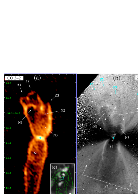
Figure 1.— The central bipolar nebula in the Boomerang (a) ALMA ¹²CO J=3–2 moment zero map (integrated over the velocity range of $-21.5<V_{lsr}\,\mbox{km~{}s${}^{-1}$}<6.5$, and (b) HST image of the 0.6µm percentage polarization. Inset (c) shows expanded view of the central region $0\farcs 65\times 0\farcs 95$ region, with contours showing the total 0.6µm intensity at 0.47, 0.87, 1.1, 3.3, and 32%, of the peak. Cyan circles in the panels mark the location of the 0.87µm continuum peak, at (J2000) RA=12:44:46.084, Dec=-54:31:13.35.

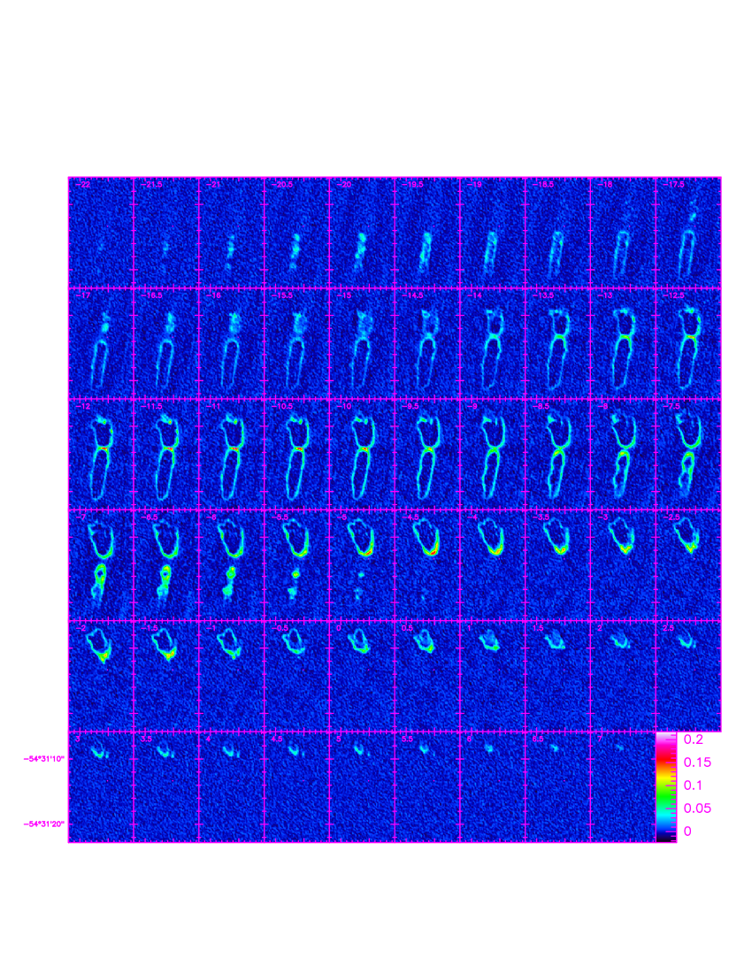
Figure 2.— CO J=3–2 channel map of the Boomerang. Intensity scale-bar units are Jy beam^-1. The 1$\sigma$ noise is $4.8\times 10^{-3}$ Jy beam^-1.

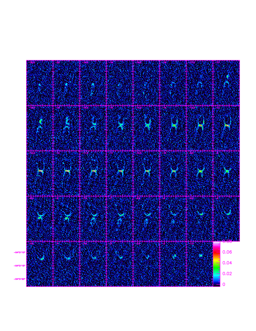
Figure 3.— ¹³CO J=3–2 channel map of the Boomerang. Intensity scale-bar units are Jy beam^-1. The 1$\sigma$ noise is $5.3\times 10^{-3}$ Jy beam^-1

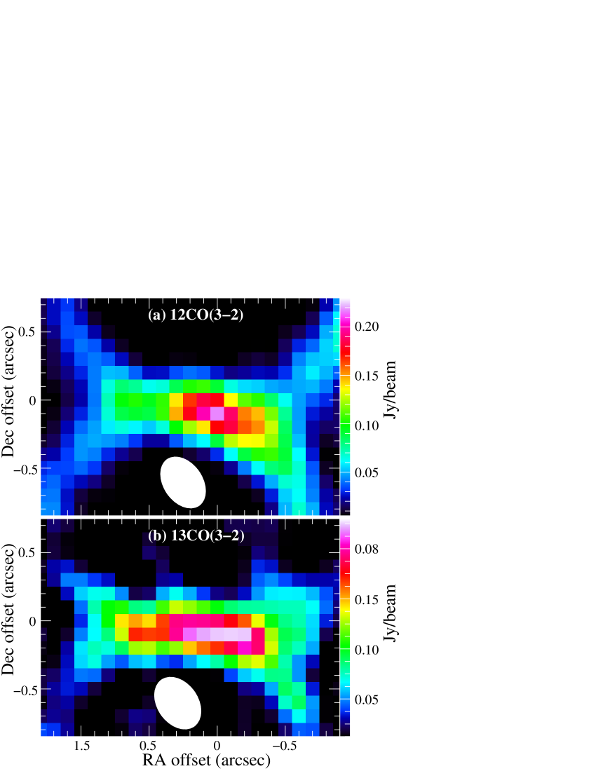
Figure 4.— The waist of the Boomerang Nebula, as seen in (a) ¹²CO J=3–2 (white ellipse: beam FWHM $0\farcs 37\times 0\farcs 25$, $PA=34.4$°), and (b) ¹³CO J=3–2 (white ellipse: beam FWHM $0\farcs 37\times 0\farcs 26$, $PA=34.4$°) images, at the central velocity of the waist emission profile, $V_{lsr}=-12$ kms.

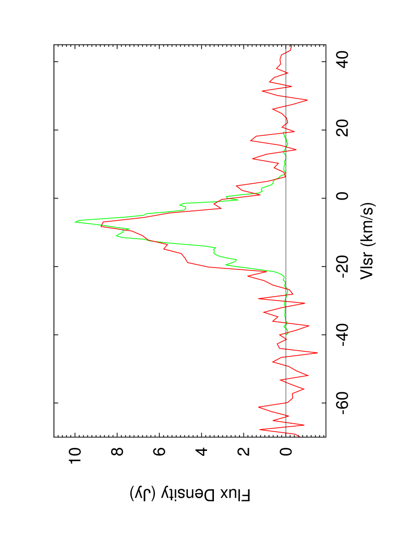
Figure 5.— Single-dish (APEX) CO J=3–2 spectrum of the Boomerang, compared to the spatially-integrated ALMA spectrum (scaled up by factor 2).

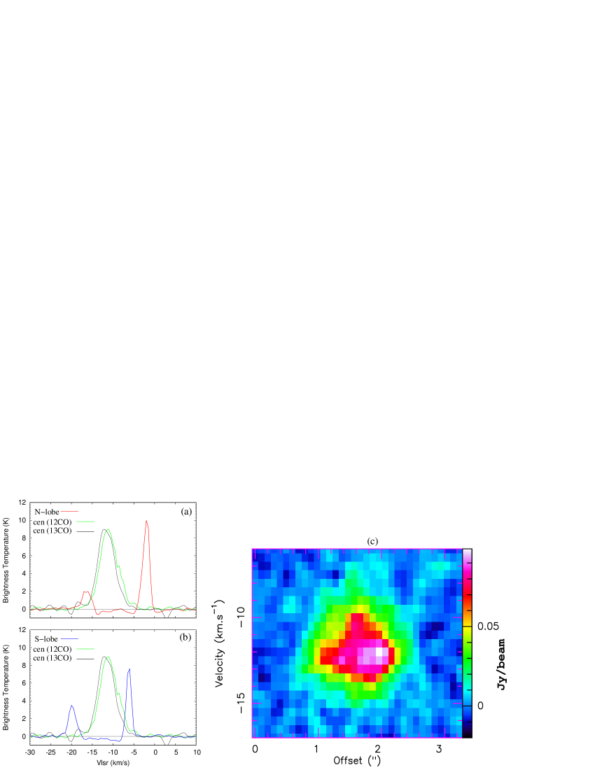
Figure 6.— (a, b) ¹²CO J=3–2 spectra extracted from the northern (red), and southern (blue) lobes of the Boomerang. The ¹²CO and ¹³CO 3–2 spectra from the central waist in green (scaled by 0.5) and black (scaled by 0.95) are shown in each panel for comparison. (c) Position-velocity cut of the ¹³CO J=3–2 intensity, taken along the major axis of the waist of the Boomerang.

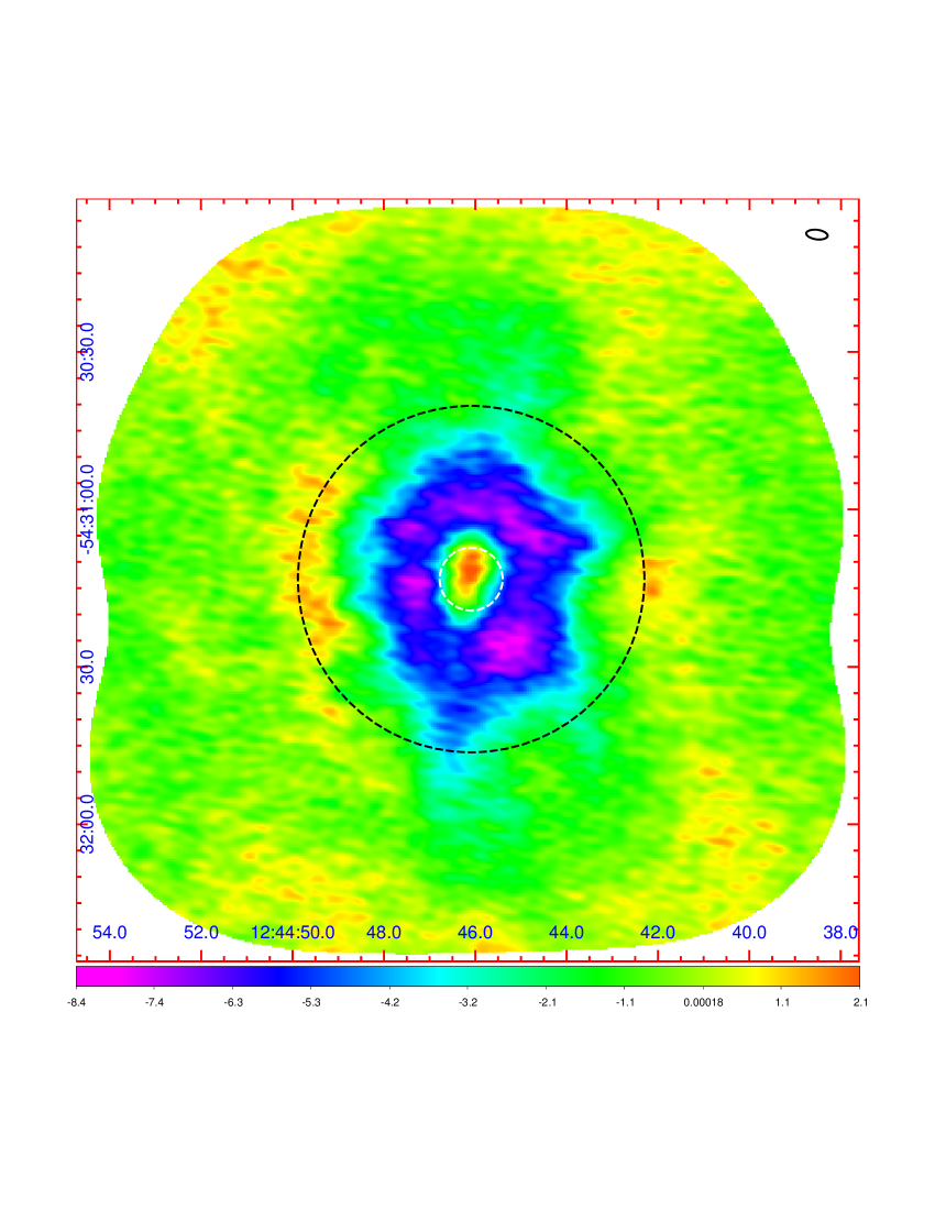
Figure 7.— CO J=1–0 moment 0 map of the Boomerang, covering the velocity range, $-171<V_{lsr}\,(\mbox{km~{}s${}^{-1}$})<144$. The black (white) dashed circle denotes the size of the SN97 model ultra-cold outflow (inner outflow). The color scale is in units of Jy-km/s beam^-1; the beam size (FWHM) is shown at the top right corner.

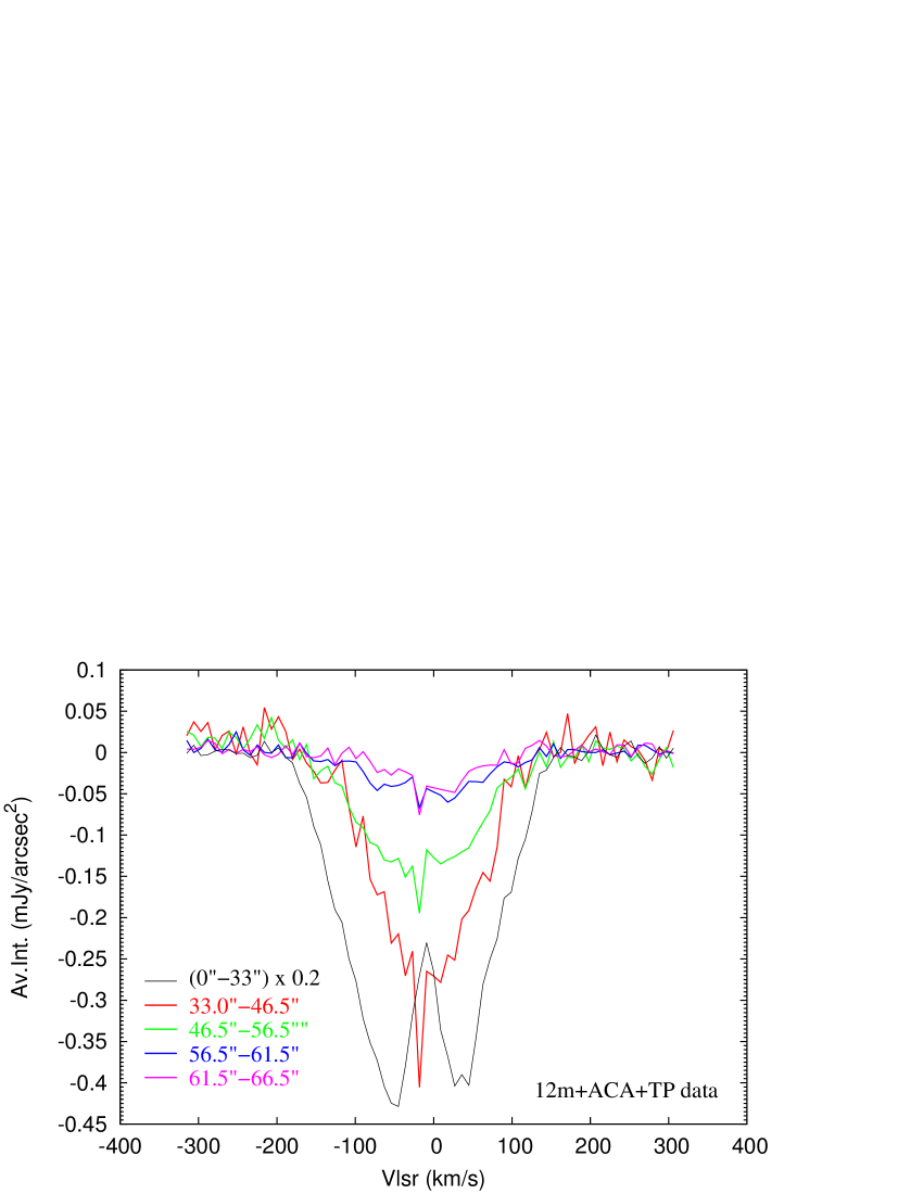
Figure 8.— CO J=1–0 spectra extracted from the combined datacube, using annular apertures of increasing average radius.

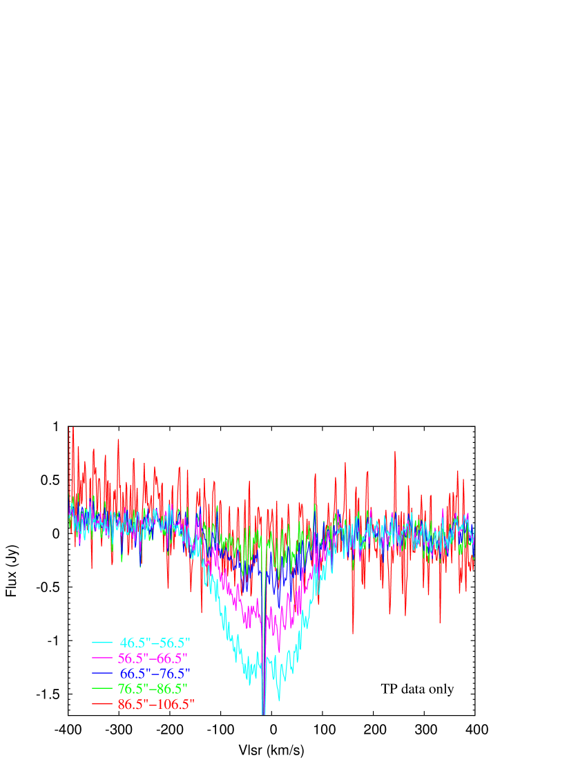
Figure 9.— CO J=1–0 spectra extracted from the TP datacube, using annular apertures of increasing average radius.

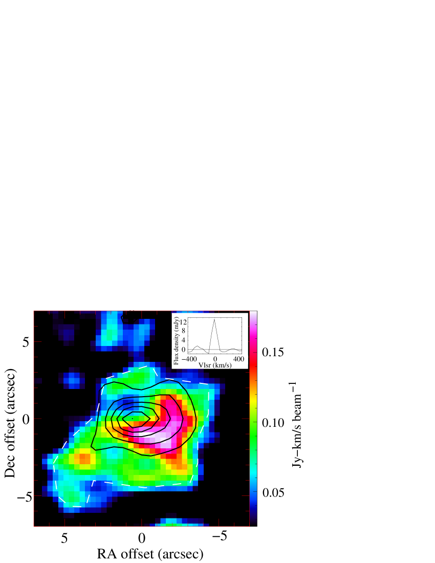
Figure 10.— Moment 0 map of the SO N,J=2,3-1,2 line emission (color-scale), overlaid with the 92 GHz continuum emission (contours) towards the Boomerang. The minimum contour (step) is 25% (15%) of the peak intensity, $3.37\times 10^{-4}$ Jy-km s^-1 beam^-1. The beam for the SO (continuum) data is $2\farcs 38\times 1\farcs 81$, $PA$=-87.4°($2\farcs 61\times 1\farcs 97$, $PA$=-89.1°). Inset shows the SO line profile, extracted from a polygonal aperture (dashed line).

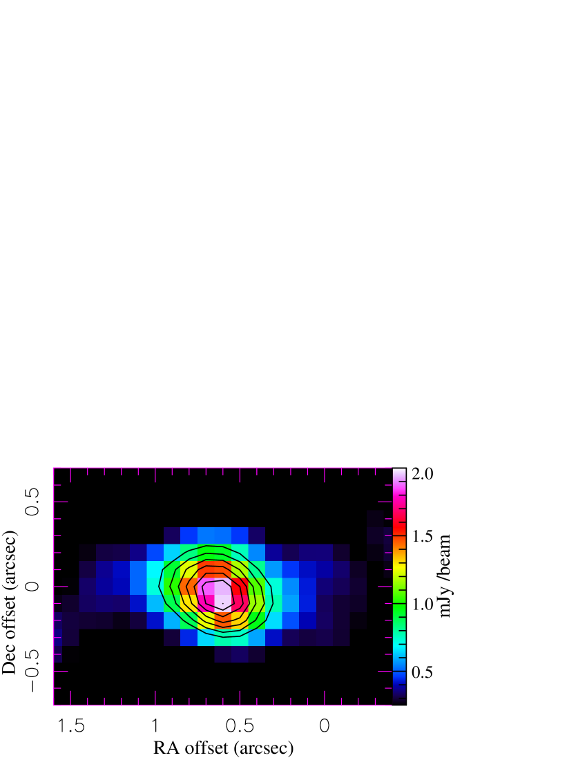
Figure 11.— The 0.87 mm continuum emission from the Boomerang. The continuum peak is located at (J2000) RA=12:44:46.081, Dec=-54:31:13.38, whereas the phase center (i.e., offset 0,0) is located at (J2000) RA=12:44:46.01, Dec=-54:31:13.32. Minimum contour level (step) is 40% (10%) of the peak, 1.96 mJy/beam. Beam (FWHM) is $0\farcs 43\,\times\,0\farcs 35$, at $PA=42.4\arcdeg$.

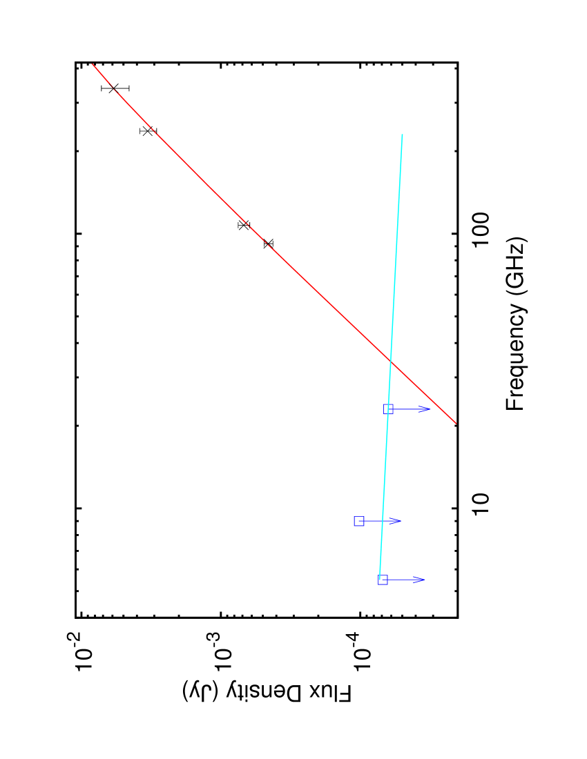
Figure 12.— The radio to millimeter-wave SED of the Boomerang. Error bars for the ALMA data (black crosses) are $\pm 1.5\sigma$. The ATCA data show (blue squares) $\pm 3\sigma$ upper limits. The ALMA data have been fitted with optically-thin dust emission from large grains with temperature 30 K and a power-law emissivity index, $\beta=0.11$ (red curve). The ATCA upper-limits have been fitted with optically-thin free-free emission (cyan curve).

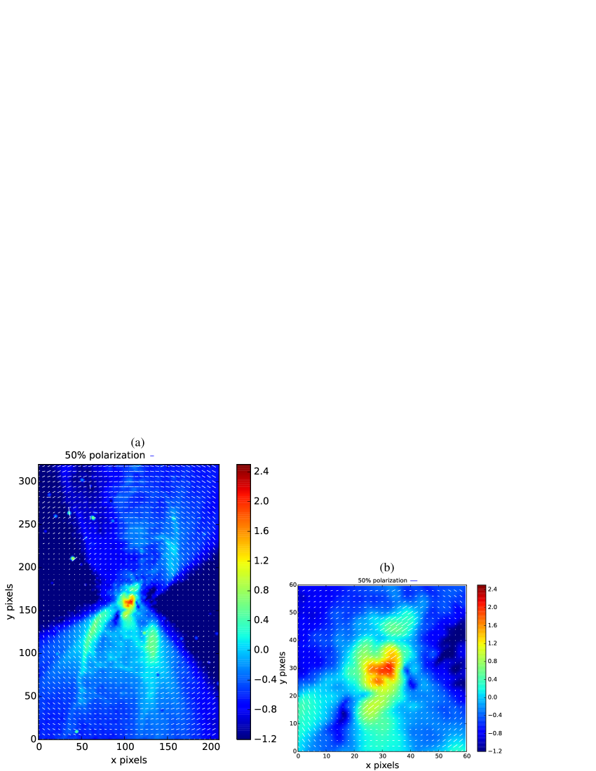
Figure 13.— Optical polarization in the Boomerang Nebula as observed with HST/ACS (a) The 0.6µm polarized light intensity image (log stretch) overlaid with vectors showing the polarization angle and percentage polarization (b) As in $a$, but for the central region. Color bars show the log of the intensity, i.e., log10(DN pixel^-1), where 1 DN $=5.016\times 10^{-19}$ erg s^-1 cm^-2 Å^-1. The angular scale is $0\farcs 025$ pixel^-1.

References

- Balick & Frank (2002) Balick, B., & Frank, A. 2002, ARA&A, 40, 439
- Bujarrabal et al. (2013) Bujarrabal, V., Alcolea, J., Van Winckel, H., Santander-García, M., & Castro-Carrizo, A. 2013, A&A, 557, A104
- Bujarrabal et al. (2012) Bujarrabal, V., Alcolea, J., Soria-Ruiz, R., et al. 2012, A&A, 537, A8
- Bujarrabal et al. (2016) Bujarrabal, V., Castro-Carrizo, A., Alcolea, J., et al. 2016, A&A, 593, A92
- Bujarrabal et al. (2017) Bujarrabal, V., Castro-Carrizo, A., Alcolea, J., et al. 2017, A&A, 597, L5
- Canovas et al. (2015) Canovas, H., Ménard, F., de Boer, J., et al. 2015, A&A, 582, L7
- Cracraft & Sparks (2007) Cracraft, M., & Sparks, W. B. 2007, Instrument Science Report ACS 2007-10
- De Marco et al. (2011) De Marco, O., Passy, J.-C., Moe, M., et al. 2011, MNRAS, 411, 2277
- de Ruyter et al. (2006) de Ruyter, S., van Winckel, H., Maas, T., et al. 2006, A&A, 448, 641
- Draine & Lazarian (1998) Draine, B. T., & Lazarian, A. 1998, ApJ, 508, 157
- Draine & Hensley (2012) Draine, B. T., & Hensley, B. 2012, ApJ, 757, 103
- Draine & Hensley (2013) Draine, B. T., & Hensley, B. 2013, ApJ, 765, 159
- Gesicki & Zijlstra (2007) Gesicki, K., & Zijlstra, A. A. 2007, A&A, 467, L29
- Groenewegen (2012) Groenewegen, M. A. T. 2012, A&A, 540, A32
- Herman, Burger & Penninx (1986) Herman, J., Burger, J.H., & Penninx, W.H. 1986, A&A, 167, 247
- Hony et al. (2002) Hony, S., Waters, L. B. F. M., & Tielens, A. G. G. M. 2002, A&A, 390, 533
- Huggins (2007) Huggins, P. J. 2007, ApJ, 663, 342
- Huggins (2012) Huggins, P. J. 2012, IAU Symposium, 283, 188
- Iaconi et al. (2017) Iaconi, R., Reichardt, T., Staff, J., et al. 2017, MNRAS, 464, 4028
- Ivanova et al. (2013) Ivanova, N., Justham, S., Chen, X., et al. 2013, A&A Rev., 21, 59
- Ivanova et al. (2015) Ivanova, N., Justham, S., & Podsiadlowski, P. 2015, MNRAS, 447, 2181
- Jura (1975) Jura, M. 1975, AJ, 80, 227
- Kamath et al. (2016) Kamath, D., Wood, P. R., Van Winckel, H., & Nie, J. D. 2016, A&A, 586, L5
- Mie (1908) Mie, G. 1908, Annalen der Physik, 330, 377
- Miller Bertolami (2016) Miller Bertolami, M. M. 2016, A&A, 588, A25
- Morris (1975) Morris, M. 1975, ApJ, 197, 603
- Pollack et al. (1994) Pollack, J. B. et al. 1994, ApJ, 421, 615
- Sahai et al. (1999) Sahai, R., Bujarrabal, V., & Zijlstra, A. 1999, ApJ, 518, L115
- Sahai et al. (2011) Sahai, R., Claussen, M. J., Schnee, S. et al. 2011, ApJ, 739, L3
- Sahai et al. (2007) Sahai, R., Morris, M., Sánchez Contreras, C., & Claussen, M. 2007, AJ, 134, 2200
- Sahai,Morris & Villar (2011) Sahai, R., Morris, M. R., & Villar, G. G. 2011, AJ, 141, 134
- Sahai et al. (1997) Sahai, R. & Nyman, L-Å., 1997, ApJ, 487, L155 (SN97)
- Sahai et al. (2013) Sahai, R., Vlemmings, W. H. T., Huggins, P. J., Nyman, L.-Å., & Gonidakis, I. 2013, ApJ, 777, 92
- Sahai et al. (2017) Sahai, R., Vlemmings, W. H. T., Gledhill, T., et al. 2017, ApJ, 835, L13
- Sahai et al. (2015) Sahai, R., Vlemmings, W., & Nyman, L.-Å. 2015, Revolution in Astronomy with ALMA: The Third Year, 499, 327
- Sahai et al. (1994) Sahai, R., Wootten, A., Schwarz, H. E., & Wild, W. 1994, ApJ, 428, 237
- Silsbee et al. (2011) Silsbee, K., Ali-Haïmoud, Y., & Hirata, C. M. 2011, MNRAS, 411, 2750
- Van der Tak et al. (2007) Van der Tak, F.F.S., Black, J.H., Schoier, F.L., Jansen, D.J., van Dishoeck, E.F., 2007, A&A 468, 627
- van Winckel et al. (2009) van Winckel, H., Lloyd Evans, T., Briquet, M., et al. 2009, A&A, 505, 1221
- Vassiliadis & Wood (1994) Vassiliadis, E., & Wood, P. R. 1994, ApJS, 92, 125
- Wegner & Glass (1979) Wegner, G. & Glass, I.S. 1979, MNRAS, 188, 327
- Winters et al. (2000) Winters, J. M., Le Bertre, T., Jeong, K. S., Helling, C., & Sedlmayr, E. 2000, A&A, 361, 641
- Woitke (2006) Woitke, P. 2006, A&A, 460, L9
- Woodward et al. (2011) Woodward, C. E., Jones, T. J., Brown, B., et al. 2011, AJ, 141, 181