Fast Spectral Ranking for Similarity Search

Abstract

Despite the success of deep learning on representing images for particular object retrieval, recent studies show that the learned representations still lie on manifolds in a high dimensional space. This makes the Euclidean nearest neighbor search biased for this task. Exploring the manifolds online remains expensive even if a nearest neighbor graph has been computed offline.

This work introduces an explicit embedding reducing manifold search to Euclidean search followed by dot product similarity search. This is equivalent to linear graph filtering of a sparse signal in the frequency domain. To speed up online search, we compute an approximate Fourier basis of the graph offline. We improve the state of art on particular object retrieval datasets including the challenging Instre dataset containing small objects. At a scale of $10^{5}$ images, the offline cost is only a few hours, while query time is comparable to standard similarity search.

1 Introduction

Image retrieval based on deep learned features has recently achieved near perfect performance on all standard datasets [45, 14, 15]. It requires fine-tuning on a properly designed image matching task involving little or no human supervision. Yet, retrieving particular small objects is a common failure case. Representing an image with several regions rather than a global descriptor is indispensable in this respect [46, 60]. A recent study [24] uses a particularly challenging dataset [67] to investigate graph-based query expansion and re-ranking on regional search.

Query expansion [7] explores the image manifold by recursive Euclidean or similarity search on the nearest neighbors (NN) at increased online cost. Graph-based methods [44, 53] help reducing this cost by computing a $k$-NN graph offline. Given this graph, random walk processes [39, 70] provide a principled means of ranking. Iscen et al. [24] transform the problem into finding a solution $\mathbf{x}$ of a linear system $A\mathbf{x}=\mathbf{y}$ for a large sparse dataset-dependent matrix $A$ and a sparse query-dependent vector $\mathbf{y}$. Such a solution can be found efficiently on-the-fly with conjugate gradients (CG). Even for an efficient solver, the query times are still in the order of one second at large scale.

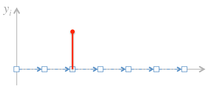
(a) Input signal $\mathbf{y}$

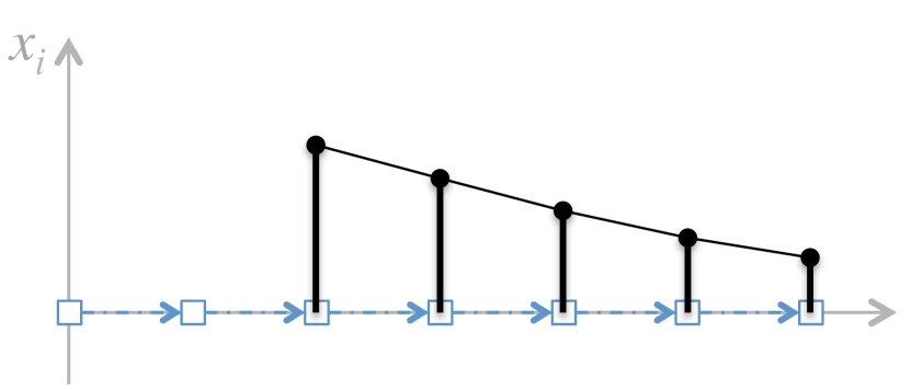
(b) Output signal $\mathbf{x}$

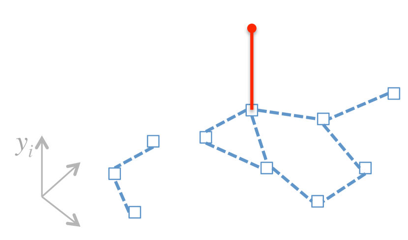
(c) Input signal $\mathbf{y}$

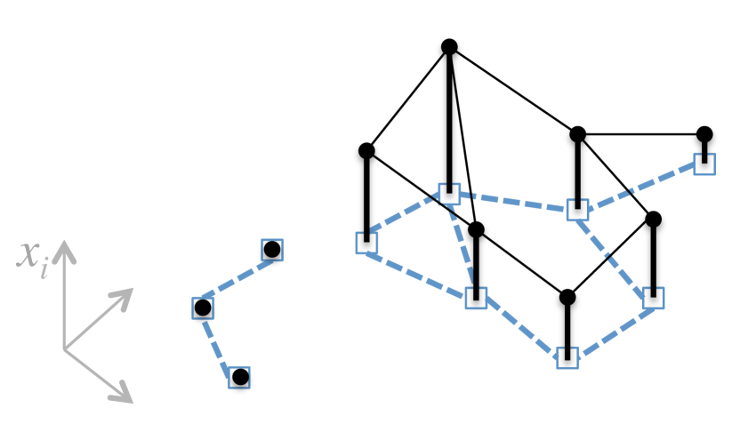
(d) Output signal $\mathbf{x}$

Figure 1: The low-pass filtering of an impulse over the real line (top) and a graph (bottom). In a weighted undirected graph the information “flows” in all directions, controlled by edge weights. In retrieval, the impulse in red is the query, and the output $\mathbf{x}$ is its similarity to all samples.

In this work, we shift more computation offline: we exploit a low-rank spectral decomposition $A\approx U\Lambda U^{\!\top}$ and express the solution in closed form as $\mathbf{x}=U\Lambda^{-1}U^{\!\top}\mathbf{y}$. We thus treat the query as a signal $\mathbf{y}$ to be smoothed over the graph, connecting query expansion to graph signal processing [50]. Figure 1 depicts 1d and graph miniatures of this interpretation. We then generalize, improve and interpret this spectral ranking idea on large-scale image retrieval. In particular, we make the following contributions:

1. We cast image retrieval as linear filtering over a graph, efficiently performed in the frequency domain.

2. We provide a truly scalable solution to computing an approximate Fourier basis of the graph offline, accompanied by performance bounds.

3. We reduce manifold search to a two-stage similarity search thanks to an explicit embedding.

4. A rich set of interpretations connects to different fields.

The text is structured as follows. Section 2 describes the addressed problem while Sections 3 and 4 present a description and an analysis of our method respectively. Section 5 gives a number of interpretations and connections to different fields. Section 6 discusses our contributions against related work. We report experimental findings in Section 8 and draw conclusions in Section 9.

2 Problem

In this section we state the problem addressed by this paper in detail. We closely follow the formulation of [24].

2.1 Representation

A set of $n$ descriptor vectors $\mathcal{V}=\{\mathbf{v}_{1},\dots,\mathbf{v}_{n}\}$, with each $\mathbf{v}_{i}$ associated to vertex $v_{i}$ of a weighted undirected graph $G$ is given as an input. The graph $G$ with $n$ vertices $V=\{v_{1},\dots,v_{n}\}$ and $\ell$ edges is represented by its $n\times n$ symmetric nonnegative adjacency matrix $W$. Graph $G$ contains no self-loops, i.e. $W$ has zero diagonal. We assume $W$ is sparse with $2\ell\ll n(n-1)$ nonzero elements.

We define the $n\times n$ degree matrix $D\mathrel{\operatorname{:=}}\operatorname{diag}(W\mathbf{1})$ where $\mathbf{1}$ is the all-ones vector, and the symmetrically normalized adjacency matrix $\mathcal{W}\mathrel{\operatorname{:=}}D^{-1/2}WD^{-1/2}$ with the convention $0/0=0$. We also define the Laplacian and normalized Laplacian of $G$ as $L\mathrel{\operatorname{:=}}D-W$ and $\mathcal{L}\mathrel{\operatorname{:=}}D^{-1/2}LD^{-1/2}=I-\mathcal{W}$, respectively. Both are singular and positive-semidefinite; the eigenvalues of $\mathcal{L}$ are in the interval $[0,2]$ [8]. Hence, if $\lambda_{1},\dots,\lambda_{n}$ are the eigenvalues of $\mathcal{W}$, its spectral radius $\varrho(\mathcal{W})\mathrel{\operatorname{:=}}\max_{i}|\lambda_{i}|$ is $1$. Each eigenvector $\mathbf{u}$ of $L$ associated to eigenvalue $0$ is constant within connected components (e.g., $L\mathbf{1}=D\mathbf{1}-W\mathbf{1}=\mathbf{0}$), while the corresponding eigenvector of $\mathcal{L}$ is $D^{1/2}\mathbf{u}$.

2.2 Transfer function

We define the $n\times n$ matrices $L_{\alpha}\mathrel{\operatorname{:=}}\beta^{-1}(D-\alpha W)$ and $\mathcal{L}_{\alpha}\mathrel{\operatorname{:=}}D^{-1/2}L_{\alpha}D^{-1/2}=\beta^{-1}(I-\alpha\mathcal{W})$, where $\alpha\in[0,1)$ and $\beta:=1-\alpha$. Both are positive-definite. Given the $n\times 1$ sparse observation vector $\mathbf{y}$ online, [24] computes the $n\times 1$ ranking vector $\mathbf{x}$ as the solution of the linear system

$$\mathcal{L}_{\alpha}\mathbf{x}=\mathbf{y}.$$ (1)

We can write the solution as $h_{\alpha}(\mathcal{W})\mathbf{y}$, where

$$h_{\alpha}(\mathcal{W})\mathrel{\operatorname{:=}}(1-\alpha)(I-\alpha\mathcal{W})^{-1}$$ (2)

for a matrix $\mathcal{W}$ such that $I-\alpha\mathcal{W}$ is nonsingular; indeed, $\mathcal{L}_{\alpha}^{-1}=h_{\alpha}(\mathcal{W})$. Here we generalize this problem by considering any given transfer function $h:\mathcal{S}\to\mathcal{S}$, where $\mathcal{S}$ is the set of real symmetric matrices including scalars, . The general problem is then to compute

$$\mathbf{x}^{*}\mathrel{\operatorname{:=}}h(\mathcal{W})\mathbf{y}$$ (3)

efficiently, in the sense that $h(\mathcal{W})$ is never explicitly computed or stored: $\mathcal{W}$ is given in advance and we are allowed to pre-process it offline, while both $\mathbf{y}$ and $h$ are given online. For $h_{\alpha}$ in particular, we look for a more efficient solution than solving linear system (1).

2.3 Retrieval application

The descriptors $\mathcal{V}$ are generated by extracting image descriptors from either whole images, or from multiple sampled rectangular image regions, which can be optionally reduced by a Gaussian mixture model as in [24]. Note that the global descriptor is a special case of the regional one, using a single region per image. In the paper, we use CNN-based descriptors [45].

The undirected graph $G$ is a $k$-NN similarity graph constructed as follows. Given two descriptors $\mathbf{v},\mathbf{z}$ in ^d, their similarity is measured as $s(\mathbf{v},\mathbf{z})=[\mathbf{v}^{\!\top}\mathbf{z}]_{+}^{\gamma}$, where exponent $\gamma>0$ is a parameter. We denote by $s(\mathbf{v}_{i}|\mathbf{z})$ the similarity $s(\mathbf{v}_{i},\mathbf{z})$ if $\mathbf{v}_{i}$ is a $k$-NN of $\mathbf{z}$ in $\mathcal{V}$ and zero otherwise. The symmetric adjacency matrix $W$ is defined as $w_{ij}\mathrel{\operatorname{:=}}\min(s(\mathbf{v}_{i}|\mathbf{v}_{j}),s(\mathbf{v}_{j}|\mathbf{v}_{i}))$, representing mutual neighborhoods. Online, given a query image represented by descriptors $\{\mathbf{q}_{1},\dots,\mathbf{q}_{m}\}\subset^{d}$, the observation vector $\mathbf{y}\in^{n}$ is formed with elements $y_{i}\mathrel{\operatorname{:=}}\sum_{j=1}^{m}s(\mathbf{v}_{i}|\mathbf{q}_{j})$ by pooling over query regions. We make $\mathbf{y}$ sparse by keeping the $k$ largest entries and dropping the rest.

3 Method

This section presents our fast spectral ranking ($\mathrm{{FSR}}$) algorithm in abstract form first, then with concrete choices.

3.1 Algorithm

We describe our algorithm given an arbitrary $n\times n$ matrix $A\in\mathcal{S}$ instead of $\mathcal{W}$. Our solution is based on a sparse low-rank approximation of $A$ computed offline such that online, $\mathbf{x}\approx h(A)\mathbf{y}$ is reduced to a sequence of sparse matrix-vector multiplications. The approximation is based on a randomized algorithm [47] that is similar to Nyström sampling [12] but comes with performance guarantees [18, 68]. In the following, $r\ll n$, $p<r$, $q$ and $\tau$ are given parameters, and $\hat{r}=r+p$.

1. (Offline) Using simultaneous iteration [62, §28], compute an $n\times\hat{r}$ matrix $Q$ with orthonormal columns that represents an approximate basis for the range of $A$, i.e. $QQ^{\!\top}A\approx A$. In particular, this is done as follows [18, §4.5]: randomly draw an $n\times\hat{r}$ standard Gaussian matrix $B^{(0)}$ and repeat for $t=0,\dots,q-1$:

   1. Compute QR factorization $Q^{(t)}R^{(t)}=B^{(t)}$.

   2. Define the $n\times\hat{r}$ matrix $B^{(t+1)}\mathrel{\operatorname{:=}}AQ^{(t)}$.

   Finally, set $Q\mathrel{\operatorname{:=}}Q^{(q-1)}$, $B\mathrel{\operatorname{:=}}B^{(q)}=AQ$.

2. (Offline–Fourier basis) Compute a rank-$r$ eigenvalue decomposition $U\Lambda U^{\!\top}\approx A$, where $n\times r$ matrix $U$ has orthonormal columns and $r\times r$ matrix $\Lambda$ is diagonal. In particular, roughly following [18, §5.3]:

   1. Form the $\hat{r}\times\hat{r}$ matrix $C\mathrel{\operatorname{:=}}Q^{\!\top}B=Q^{\!\top}AQ$.

   2. Compute its eigendecomposition $\hat{V}\hat{\Lambda}\hat{V}^{\!\top}=C$.

   3. Form $(V,\Lambda)$ by keeping from $(\hat{V},\hat{\Lambda}$) the slices (rows/columns) corresponding to the $r$ largest eigenvalues.

   4. Define the matrix $U\mathrel{\operatorname{:=}}QV$.

3. (Offline) Make $U$ sparse by keeping its $\tau$ largest entries and dropping the rest.

4. (Online) Given $\mathbf{y}$ and $h$, compute

   $$\mathbf{x}\mathrel{\operatorname{:=}}Uh(\Lambda)U^{\!\top}\mathbf{y}.$$ (4)

Observe that $U^{\!\top}$ projects $\mathbf{y}$ onto ^r. With $\Lambda$ being diagonal, $h(\Lambda)$ is computed element-wise. Finally, multiplying by $U$ and ranking $\mathbf{x}$ amounts to dot product similarity search in ^r. The online stage is very fast, provided $U$ only contains few leading eigenvectors and $\mathbf{y}$ is sparse. We consider the following variants:

• $\mathrm{{FSR}}$.sparse: This is the complete algorithm.

• $\mathrm{{FSR}}$.approx: Drop sparsification stage 3.

• $\mathrm{{FSR}}$.rank-${r}$: Drop approximation stage 1 and sparsification stage 3. Set $\hat{r}=n$, $Q=I$, $B=A$ in stage 2.

• $\mathrm{{FSR}}$.exact: same as $\mathrm{{FSR}}$.rank-${r}$ for $r=n$.

To see why $\mathrm{{FSR}}$.exact works, consider the case of $h_{\alpha}(\mathcal{W})$. Let $\mathcal{W}\simeq U\Lambda U^{\!\top}$. It follows that $h_{\alpha}(\mathcal{W})/\beta=(I-\alpha\mathcal{W})^{-1}\simeq U(I-\alpha\Lambda)^{-1}U^{\!\top}$, where $(I-\alpha\Lambda)^{-1}$ is computed element-wise. Then, $\mathbf{x}^{*}\simeq\beta U(I-\alpha\Lambda)^{-1}U^{\!\top}\mathbf{y}$. The general case is discussed in section 4.

3.2 Retrieval application

Returning to the retrieval problem, we compute the ranking vector $\mathbf{x}\in^{n}$ by (4), containing the ranking score $x_{i}$ of each dataset region $\mathbf{v}_{i}$. To obtain a score per image, we perform a linear pooling operation [24] represented as $\overline{\mathbf{x}}\mathrel{\operatorname{:=}}\Sigma\mathbf{x}$ where $\Sigma$ is a sparse $N\times n$ pooling matrix. The $N\times r$ matrix $\overline{U}\mathrel{\operatorname{:=}}\Sigma U$ is indeed computed offline so that we directly compute $\overline{\mathbf{x}}=\overline{U}h(\Lambda)U^{\!\top}\mathbf{y}$ online.

Computing $\mathbf{y}$ involves Euclidean search in ^d, which happens to be dot product because vectors are $\ell^{2}$-normalized. Applying $\overline{U}$ and ranking $\mathbf{x}$ amounts to a dot product similarity search in ^r. We thus reduce manifold search to Euclidean followed by dot product search. The number of nonzero elements of $\mathbf{y}$ and rows of $\overline{U}$, whence the cost, are the same for global or regional search.

4 Analysis

We derive the asymptotic space and time complexity of different algorithm variants and derive necessary condition for correctness and error bounds of approximate variants.

4.1 Complexity

The offline complexity is mainly determined by the number of columns $\hat{r}$ of matrix $Q$: Stage 1 reduces the size of the problem from $n^{2}$ down to $n\hat{r}$. The online complexity is determined by the number of nonzero entries in matrix $U$. A straightforward analysis leads to the following:

• $\mathrm{{FSR}}$.approx: The offline complexity is $O(qn(k+\hat{r})\hat{r})$ time and $O(n\hat{r})$ space; its online (time and space) complexity is $O(nr)$.

• $\mathrm{{FSR}}$.sparse: The offline complexity is $O(qn(k+\hat{r})\hat{r}+\tau\log\tau)$ time and $O(n\hat{r})$ space; its online complexity is $O(\tau)$.

Stage 1 is “embarrassingly parallelizable” meaning that it is dramatically accelerated on parallel and distributed platforms. Since the online stage 4 amounts to NN search, any approximate method applies, making it sublinear in $n$.

4.2 Correctness

We derive here the conditions on $h$ and $A$ under which our algorithm is correct under no truncation, i.e., $\mathrm{{FSR}}.\textsc{exact}(\mathbf{y}|A,h)=h(A)\mathbf{y}$. We also show, that $h_{\alpha}$ and $\mathcal{W}$ satisfy these conditions, which is an alternative proof of correctness to the one in Section 3.1.

Starting from the fact a real symmetric matrix $A$ is diagonalizable, there exists an exact eigenvalue decomposition $U\Lambda U^{\!\top}=A$, where $U$ is orthogonal. According to [1, §9.14,9.2], we have $h(A)=Uh(\Lambda)U^{\!\top}=U\operatorname{diag}(h(\lambda_{1}),\dots,h(\lambda_{n}))U^{\!\top}$ if and only if there exists a series expansion of $h$ converging for this specific $A$:

$$h(A)=\sum_{t=0}^{\infty}c_{t}A^{t}.$$ (5)

This holds in particular for $h_{\alpha}$ admitting the geometric progression expansion

$$h_{\alpha}(A)\mathrel{\operatorname{:=}}\beta(I-\alpha A)^{-1}=\beta\sum_{t=0}^{\infty}(\alpha A)^{t},$$ (6)

which converges absolutely if $\varrho(\alpha A)<1$ [1, §9.6,9.19]. This holds for $A=\mathcal{W}$ because $\alpha<1$ and $\varrho(\mathcal{W})=1$.

4.3 Error bound

We present main ideas for bounding the approximation error of $\mathrm{{FSR}}$.rank-${r}$ and $\mathrm{{FSR}}$.approx coming from literature, and we derive another condition on $h$ under which our algorithm is valid under truncation. The approximation $QQ^{\!\top}A\approx A$ of stage 1 is studied in [18, §9.3,10.4]: an average-case bound on $\left\|{A-QQ^{\!\top}A}\right\|$ decays exponentially fast in the number of iterations $q$ to $|\lambda_{r+1}|$. Stage 2 yields an approximate eigenvalue decomposition of $A$: Since $A$ is symmetric, $A\approx QQ^{\!\top}AQQ^{\!\top}=QCQ^{\!\top}\approx QV\Lambda V^{\!\top}Q^{\!\top}=U\Lambda U^{\!\top}$. The latter approximation $C\approx V\Lambda V^{\!\top}$ is essentially a best rank-$r$ approximation of $C=Q^{\!\top}AQ$. This is also studied in [18, §9.4] for the truncated SVD case of a non-symmetric matrix. It involves an additional term of $|\lambda_{r+1}|$ in the error.

We are actually approximating $h(A)$ by $Uh(\Lambda)U^{\!\top}$, so that $|h(\lambda_{r+1})|$ governs the error instead of $|\lambda_{r+1}|$. A similar situation appears in [61, §3.3]. Therefore, our method makes sense only when the restriction of $h$ to scalars is nondecreasing. This is the case for $h_{\alpha}$.

5 Interpretation

Our work is connected to studies in different fields with a long history. Here we give a number of interpretations both in general and in the particular case $h=h_{\alpha}$.

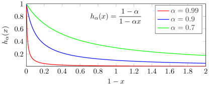
Figure 2: Function $h_{\alpha}$ (2) is a ‘low-pass filter’; $1-x$ represents eigenvalues of $\mathcal{L}$, where $0$ is the DC component.

5.1 Graph signal processing

In signal processing [38], a discrete-time signal of period $n$ is a vector $\mathbf{s}\in^{n}$ where indices are represented by integers modulo $n$, that is, $s_{\bar{i}}\mathrel{\operatorname{:=}}s_{(i\bmod n)+1}$ for $i\in\mathbb{Z}$. A shift (or translation, or delay) of $\mathbf{s}$ by one sample is the mapping $s_{\bar{i}}\mapsto s_{\overline{i-1}}$. If we define the $n\times n$ circulant matrix $C_{n}\mathrel{\operatorname{:=}}(\mathbf{e}_{2}\ \mathbf{e}_{3}\dots\mathbf{e}_{n}\ \mathbf{e}_{1})$, a shift can be represented by $\mathbf{s}\mapsto C_{n}\mathbf{s}$ [50]. A linear, time (or shift) invariant filter is the mapping $\mathbf{s}\mapsto H\mathbf{s}$ where $H$ is an $n\times n$ matrix with a series representation $H\mathrel{\operatorname{:=}}h(C_{n})=\sum_{t=0}^{\infty}h_{t}C_{n}^{t}$. Matrix $C_{n}$ has the eigenvalue decomposition $U\Lambda U^{\!\top}$ where $U^{\!\top}$ is the $n\times n$ discrete Fourier transform matrix $\mathcal{F}$. If the series $h(C_{n})$ converges, filtering $\mathbf{s}\mapsto H\mathbf{s}$ is written as

$$\mathbf{s}\mapsto\mathcal{F}^{-1}h(\Lambda)\mathcal{F}\mathbf{s}.$$ (7)

That is, $\mathbf{s}$ is mapped to the frequency domain, scaled element-wise, and mapped back to the time domain.

Graph signal processing [50, 54] generalizes the above concepts to graphs by replacing $C_{n}$ by $\mathcal{W}$, an appropriately normalized adjacency matrix of an arbitrary graph. If $U\Lambda U^{\!\top}$ is the eigenvalue decomposition of $\mathcal{W}$, we realize that (4) treats $\mathbf{y}$ as a (sparse) signal and filters it in the frequency domain via transfer function $h$ to obtain $\mathbf{x}$. Function $h_{\alpha}$ in particular is a low-pass filter, as illustrated in Figure 2. By varying $\alpha$ from $0$ to $1$, the frequency response varies from all-pass to sharp low-pass.

5.2 Random walks

Consider the iterating process: for $t=1,2,\dots$

$$\mathbf{x}^{(t)}\mathrel{\operatorname{:=}}\alpha A\mathbf{x}^{(t-1)}+(1-\alpha)\mathbf{y}.$$ (8)

If $A$ is a stochastic transition matrix and $\mathbf{x}^{(0)},\mathbf{y}$ are distributions over vertices, this specifies a random walk on a (directed) graph: at each iteration a particle moves to a neighboring vertex with probability $\alpha$ or jumps to a vertex according to distribution $\mathbf{y}$ with probability $1-\alpha$. This is called a Markov chain with restart [2] or random walk with restart [40]. State $\mathbf{x}^{(t)}$ converges to $\mathbf{x}^{*}=h_{\alpha}(A)\mathbf{y}$ as $t\to\infty$ provided $\varrho(\alpha A)<1$ [69]. In fact, (8) is equivalent to Jacobi solver [17] on linear system (1) [24].

If $\mathbf{y}=\mathbf{e}_{i}$, the $i$-th canonical vector, then $\mathbf{x}^{*}$ is used to rank the vertices of $G$, expressing a measure of “similarity” to $v_{i}$ [70]. Parameter $\alpha$ controls how much $\mathbf{x}^{*}$ is affected by boundary condition $\mathbf{y}$ [64]: $\mathbf{x}^{*}$ equals $\mathbf{y}$ for $\alpha=0$, while in the limit $\alpha\to 1$, $\mathbf{x}^{*}$ tends to a dominant eigenvector of $A$. Indeed, for $\alpha=1$, (8) becomes a power iteration.

5.3 Random fields

Given a positive-definite $n\times n$ precision matrix $A\in\mathcal{S}$ and a mean vector $\boldsymbol{\mu}\in^{n}$, a Gaussian Markov random field (GMRF) [49] with respect to an undirected graph $G$ is a random vector $\mathbf{x}\in^{n}$ with normal density $p(\mathbf{x})\mathrel{\operatorname{:=}}\mathcal{N}(\mathbf{x}|\boldsymbol{\mu},A^{-1})$ iff $A$ has the same nonzero off-diagonal entries as the adjacency matrix of $G$. Its canonical parametrization $p(\mathbf{x})\propto e^{-E(\mathbf{x}|\mathbf{b},A)}$ where $E(\mathbf{x}|\mathbf{b},A)\mathrel{\operatorname{:=}}\frac{1}{2}\mathbf{x}^{\!\top}A\mathbf{x}-\mathbf{b}^{\!\top}\mathbf{x}$ is a quadratic energy. Its expectation $\boldsymbol{\mu}=A^{-1}\mathbf{b}$ is the minimizer of this energy. Now, $\mathbf{x}^{*}=\mathcal{L}_{\alpha}^{-1}\mathbf{y}$ (1) is the expectation of a GMRF with energy

$$f_{\alpha}(\mathbf{x})\mathrel{\operatorname{:=}}E(\mathbf{x}|\mathbf{y},\mathcal{L}_{\alpha})=\frac{1}{2}\mathbf{x}^{\!\top}\mathcal{L}_{\alpha}\mathbf{x}-\mathbf{y}^{\!\top}\mathbf{x}.$$ (9)

A mean field method on this GMRF is equivalent to Jacobi or Gauss-Seidel solvers on (1) [66]. Yet, conjugate gradients (CG) [37] is minimizing $f_{\alpha}(\mathbf{x})$ more efficiently [24, 5].

If we expand $f_{\alpha}(\mathbf{x})$ using $\beta\mathcal{L}_{\alpha}=\alpha\mathcal{L}+(1-\alpha)I$, we find that it has the same minimizer as

$$\alpha\sum_{i,j}w_{ij}\left\|{\hat{x}_{i}-\hat{x}_{j}}\right\|^{2}+(1-\alpha)\left\|{\mathbf{x}-\mathbf{y}}\right\|^{2},$$ (10)

where $\hat{\mathbf{x}}\mathrel{\operatorname{:=}}D^{-1/2}\mathbf{x}$. The pairwise smoothness term encourages $\mathbf{x}$ to vary little across edges with large weight whereas the unary fitness term to stay close to observation $\mathbf{y}$ [69]. Again, $\alpha$ controls the trade-off: $\mathbf{x}^{*}$ equals $\mathbf{y}$ for $\alpha=0$, while for $\alpha\to 1$, $\mathbf{x}^{*}$ tends to be constant over connected components like dominant eigenvectors of $\mathcal{W}$.

5.4 Regularization and kernels

The first term of (9) is interpreted as a regularization operator related to a kernel $K=\mathcal{L}_{\alpha}^{-1}$ [58, 57, 31]. In a finite graph, a kernel can be seen either as an $n\times n$ matrix $K$ or a function $\kappa:V^{2}\to$ operating on pairs of vertices. More generally, if $h(x)>0$ for $x\in$, which holds for $h_{\alpha}$, then $K\mathrel{\operatorname{:=}}h(\mathcal{W})$ is positive-definite and there is an $n\times n$ matrix $\Phi$ such that $K=\Phi^{\!\top}\Phi$, or $\kappa(v_{i},v_{j})=\phi(v_{i})^{\!\top}\phi(v_{j})$ where feature map $\phi:V\to^{n}$ is given by $\phi(v_{i})\mathrel{\operatorname{:=}}\Phi\mathbf{e}_{i}$. A particular choice for $\Phi$ is

$$\Phi\mathrel{\operatorname{:=}}h(\Lambda)^{1/2}U^{\!\top}$$ (11)

where $U\Lambda U^{\!\top}$ is the eigenvalue decomposition of $\mathcal{W}$. If we choose a rank-$r$ approximation instead, then $\Phi$ is an $r\times n$ matrix and $\phi$ is a low-dimensional embedding onto ^r.

The goal of out-of-sample extension is to compute a “similarity” $\hat{\kappa}(\mathbf{z}_{1},\mathbf{z}_{2})$ between two unseen vectors $\mathbf{z}_{1},\mathbf{z}_{2}\in^{d}$ not pertaining to the graph. Here we define

$$\hat{\kappa}(\mathbf{z}_{1},\mathbf{z}_{2})\mathrel{\operatorname{:=}}\psi(\mathbf{z}_{1})^{\!\top}\Phi^{\!\top}\Phi\psi(\mathbf{z}_{2})$$ (12)

given any mapping $\psi:^{d}\to^{n}$, e.g. $\psi(\mathbf{z})_{i}\mathrel{\operatorname{:=}}s(\mathbf{v}_{i}|\mathbf{z})$ discussed in section 2. This extended kernel is also positive-definite and its embedding $\hat{\phi}(\mathbf{z})=\Phi\psi(\mathbf{z})$ is a linear combination of the dataset embeddings. For $r\ll n$, our method allows rapid computation of $\kappa$ or $\hat{\kappa}$ for any given function $h$, without any dense $n\times n$ matrix involved.

5.5 Paths on graphs

Many nonlinear dimension reduction methods replace Euclidean distance with an approximate geodesic distance, assuming the data lie on a manifold [33]. This involves the all-pairs shortest path (APSP) problem and Dijkstra’s algorithm is a common choice. Yet, it is instructive to consider a naïve algorithm [9, §25.1]. We are given a distance matrix where missing edges are represented by $\infty$ and define similarity weight $w_{ij}=e^{-d_{ij}}$. A path weight is a now a product of similarities and “shortest” means “of maximum weight”. Defining matrix power $A^{\otimes t}$ as $A^{t}$ with $+$ replaced by $\max$, the algorithm is reduced to computing $\max_{t}W^{\otimes t}$ (element-wise). Element $i,j$ of $W^{\otimes t}$ is the weight of the shortest path of length $t$ between $v_{i},v_{j}$.

Besides their complexity, shortest paths are sensitive to changes in the graph. An alternative is the sum of weights over paths of length $t$, recovering the ordinary matrix power $\mathcal{W}^{t}$, and the weighted sum over all lengths $\sum_{t=0}^{\infty}c_{t}\mathcal{W}^{t}$, where coefficients $(c_{t})_{t\in\mathbb{N}}$ allow for convergence [64], [52, §9.4]. This justifies (5) and reveals that coefficients control the contribution of paths depending on length. A common choice is $c_{t}=\beta\alpha^{t}$ with $\beta=1-\alpha$ and $\alpha\in[0,1)$ being a damping factor [64], which justifies function $h_{\alpha}$ (6).

6 Related work

The history of the particular case $h=h_{\alpha}$ is the subject of the excellent study of spectral ranking [64]. The fundamental contributions originate in the social sciences and include the eigenvector formulation by Seeley [51], damping by $\alpha$ (6) by Katz [29] and the boundary condition $\mathbf{y}$ (1) by Hubbell [22]. The most well-known follower is PageRank [39]. In machine learning, $h_{\alpha}$ has been referred to as the von Neumann [27, 52] or regularized Laplacian kernel [57]. Along with the diffusion kernel [32, 31], it has been studied in connection to regularization [58, 57].

Random fields are routinely used for low-level vision tasks where one is promoting smoothness while respecting a noisy observation, like in denoising or segmentation, where both the graph and the observation originate from a single image [59, 5]. A similar mechanism appears in semi-supervised learning [69, 73, 71, 6] or interactive segmentation [16, 30] where the observation is composed of labels over a number of samples or pixels. In our retrieval scenario, the observation is formed by the neighbors in the graph of an external query image (or its regions).

The random walk or random walk with restart (RWR) formulation [70, 69, 40] is an alternative interpretation to retrieval [11]. Yet, directly solving a linear system is superior [24]. Offline matrix decomposition has been studied for RWR [61, 13, 26]. All three methods are limited to $h_{\alpha}$ while sparse LU decomposition [13, 26] assumes an uneven distribution of vertex degrees [28], which is not the case for $k$-NN graphs. In addition, we reduce manifold search to two-stage Euclidean search via an explicit embedding, which is data dependent through the kernel $K=\mathcal{L}_{\alpha}^{-1}$.

In the general case, the spectral formulation (4) has been known in machine learning [6, 52, 36, 72, 65] and in graph signal processing [50, 54, 19]. The latter is becoming popular in the form of graph-based convolution in deep learning [4, 21, 10, 3, 34, 43]. However, with few exceptions [4, 21], which rely on an expensive decomposition, there is nothing spectral when it comes to actual computation. It is rather preferred to work with finite polynomial approximations of the graph filter [10, 3] using Chebyshev polynomials [19, 55] or translation-invariant neighborhood templates in the spatial domain [34, 43].

We cast retrieval as graph filtering by constructing an appropriate observation vector. We actually perform the computation in the frequency domain via a scalable solution. Comparing to other applications, retrieval conveniently allows offline computation of the graph Fourier basis and online reuse to embed query vectors. An alternative is to use random projections [63, 48]. This roughly corresponds to a single iteration of our step 1. Our solution is thus more accurate, while $h$ is specified online.

7 Practical considerations

Block diagonal case. Each connected component of $G$ has a maximal eigenvalue $1$. These maxima of small components dominate the eigenvalues of the few (or one) “giant” component that contain the vast majority of data [28]. For this reason we find the connected components with the union-find algorithm [9] and reorder vertices such that $A$ is block diagonal: $A=\operatorname{diag}(A_{1},\ldots,A_{c})$. For each $n_{l}\times n_{l}$ matrix $A_{l}$, we apply offline stages 1-3 to obtain an approximate rank-$r_{l}$ eigenvalue decomposition $\hat{U}_{l}\hat{\Lambda}_{l}\hat{U}_{l}^{\!\top}\approx A_{l}$ with $r_{l}=\max(\rho,\left\lceil{rn_{l}/n}\right\rceil)$ if $n_{l}>\rho$, otherwise we compute an exact decomposition. Integer $\rho$ is a given parameter. We form $(U_{l},\Lambda_{l})$ by keeping up to $\rho$ slices from each pair $(\hat{U}_{l},\hat{\Lambda}_{l})$ and complete with up to $r$ slices in total, associated to the largest eigenvalues of the entire set $\operatorname{diag}(\hat{\Lambda}_{1},\dots,\hat{\Lambda}_{c})$. Online, we partition $(\mathbf{y}_{1};\dots;\mathbf{y}_{c})=\mathbf{y}$, compute each $\mathbf{x}_{l}$ from $\mathbf{y}_{l}$ by (4) and form back vector $\mathbf{x}=(\mathbf{x}_{1};\dots;\mathbf{x}_{c})$.

Sparse neighborhoods. Denote by $\eta_{i}$ the $\ell_{2}$-norm of the $i$-th row of $U$. $\mathrm{{FSR}}$.exact yields $\boldsymbol{\eta}=\mathbf{1}$ but this is not the case for $\mathrm{{FSR}}.\textsc{rank-}{r}$. Larger (smaller) values appear to correspond to densely (sparsely) populated parts of the graph. For small rank $r$, norms $\eta_{i}$ are more severely affected for uncommon vectors in the dataset. We propose replacing each element $x_{i}$ of (4) by

$$x^{\prime}_{i}=x_{i}+(1-\eta_{i})\mathbf{v}_{i}^{\top}\mathbf{q},$$ (13)

for global descriptors, with a straightforward extension for regional ones. This is referred to as $\mathrm{{FSRw}}$ and is a weighted combination of manifold search and Euclidean search. It approaches the former for common elements and to the latter for uncommon ones. Our experiments show that this is essential at large scale.

8 Experiments

This section introduces our experimental setup, investigates the performance and behavior of the proposed method and its application to large-scale image retrieval.

8.1 Experimental Setup

Datasets. We use three image retrieval benchmarks: Oxford Buildings (Oxford5k) [41], Paris (Paris6k) [42] and Instre [67], with the evaluation protocol introduced in [24] for the latter. We conduct large-scale experiments by following a standard protocol of adding 100k distractor images from Flickr [41] to Oxford5k and Paris6k, forming the so called Oxford105k and Paris106k. Mean average precision (mAP) evaluates the retrieval performance in all datasets.

Image Descriptors. We apply our method on the same global and regional image descriptors as in [24]. In particular, we work with $d$-dimensional vectors extracted from VGG [56] ($d=512$) and ResNet101 [20] ($d=2,048$) networks fine-tuned specifically for image retrieval [45, 15]. Global description is R-MAC with 3 different scales [60], including the full image as a separate region. Regional descriptors consist of the same regions as those involved in R-MAC but without sum pooling, resulting in 21 vectors per image on average. Global and regional descriptors are processed by supervised whitening [45].

Implementation. We adopt the same parameters for graph construction and search as in [24]. The pairwise descriptor similarity is defined as $s(\mathbf{v},\mathbf{z})=[\mathbf{v}^{\!\top}\mathbf{z}]_{+}^{3}$. We use $\alpha=0.99$, and keep the top $k=50$ and $k=200$ mutual neighbors in the graph for global and regional vectors, respectively. These choices make our experiments directly comparable to prior results on manifold search for image retrieval with CNN-based descriptors [24]. In all our $\mathrm{{FSR}}$.approx experiments, we limit the algorithm within the largest connected component only, while each element $x_{i}$ for vertex $v_{i}$ in any other component is just copied from $y_{i}$. This choice works well because the largest component holds nearly all data in practice. Following [24], generalized max-pooling [35, 23] is used to pool regional diffusion scores per image. Reported search times exclude the construction of the observation vector $\mathbf{y}$, since this task is common to all baseline and our methods. Time measurements are reported with a 4-core Intel Xeon 2.00GHz CPU.

8.2 Retrieval Performance

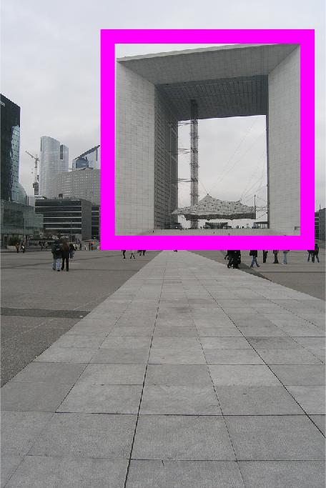
(La Défense, AP: 92.1)	#5	#32	#51	#70	#71	#76	#79	#126
(Pyramide du Louvre, AP: 92.7)	#2	#4	#8	#61	#68	#72	#75	#108

Figure 3: Two queries with the lowest AP from Paris6k (left) and the corresponding top-ranked negative images based on the ground-truth, with their rank underneath. Ranks are marked in blue for incorrectly labeled images, and red otherwise.

Figure 4: Performance of regional search with $\mathrm{{FSR}}$.rank-${r}$. Runtimes are reported in text labels. $\diamond$ refers to $\mathrm{{FSR}}$.exact performed with conjugate gradients as in [24]

Rank-$r$. We evaluate the performance of $\mathrm{{FSR}}$.rank-${r}$ for varying rank $r$, which affects the quality of the approximation and defines the dimensionality of the embedding space. As shown in Figure 4, the effect of $r$ depends on the dataset. In all cases the optimal performance is already reached at $r=1$k. On Paris6k in particular, this happens as soon as $r=100$. Compared to $\mathrm{{FSR}}$.exact as implemented in [24], it achieves the same mAP but 150 times faster on Oxford5k and Paris6k and 300 times faster on Instre. Global search demonstrates a similar behavior.

We achieve $97.0$ mAP on Paris6k, which is near-perfect. Figure 3 shows the two queries with the lowest AP and their top-ranked negative images. In most cases the ground-truth is incorrect, as these images have visual overlap with the query bounding box. The first correct negative image for “La Défense” appears at rank $126$, where buildings from the surroundings are retrieved due to “topic drift”. The same happens with “Pyramide du Louvre”, where the first correct negative image is at rank $108$.

Regional search performs better than global [24] at the cost of more memory and slower query. We unlock this bottleneck thanks to the offline pooling $\overline{U}=\Sigma U$. Indeed, global and regional search on Instre take $0.040s$ and $0.042s$ respectively with our method, while the corresponding times for $\mathrm{{FSR}}$.exact are $0.055s$ and $3s$.

Approximate eigendecomposition keeps the off-line stage tractable at large scale. With 570k regional descriptors on Instre, $\mathrm{{FSR}}$.rank-${5000}$ and $\mathrm{{FSR}}$.approx yield a mAP of $89.5$ and $89.2$ respectively, with offline cost 60 and 3 hours respectively, using 16-core Intel Xeon 2.00GHz CPU. This is important at large scale because the off-line complexity of $\mathrm{{FSR}}$.rank-${r}$ is polynomial.

When new images are added, one can express them according to existing ones, as in (12). We evaluate such extension by constructing the graph on a random subset of $100\%$, $90\%$, $70\%$, $50\%$, $30\%$ and $10\%$ of Instre, yielding $80.5$, $80.1$, $78.3$, $75.8$, $70.2$ and $40.6$ mAP respectively on the entire dataset, with global search. The drop is graceful until $30\%$; beyond that, the graph needs to be updated.

8.3 Large-scale experiments

We now apply our approach to a larger scale by using only $5$ descriptors per image using GMM reduction [24]. This choice improves scalability while minimizing the accuracy loss.

Figure 5: mAP vs. $r$ on Oxford105k with $\mathrm{{FSR}}$.approx and $\mathrm{{FSRw}}$.approx, using Resnet101(R) and VGG(V).

Figure 6: mAP vs. rank $r$ separately per landmark in Oxford105k with $\mathrm{{FSR}}$.approx (left) and $\mathrm{{FSRw}}$.approx (right). Number of positive images per landmark is shown in the legend.

$\mathrm{{FSRw}}$.approx becomes crucial, especially at large scale, because vectors of sparsely populated parts of the graph are not well represented. Figure 5 shows the comparison between $\mathrm{{FSRw}}$.approx and $\mathrm{{FSR}}$.approx. We achieve $90.2$ and $94.2$ with $\mathrm{{FSR}}$.approx and $\mathrm{{FSRw}}$.approx respectively, with $r=10$k and Resnet101 descriptors.

We further report the performance separately for each of the 11 queries of Oxford105k dataset. Results are shown in Figure 6. Low values of $r$ penalize sparsely populated parts of the graph, i.e. landmarks with less similar instances in the dataset. $\mathrm{{FSRw}}$.approx partially solves this issue.

The search time is $0.14$s and $0.3$s per query for $r=5$k and $r=10$k respectively on Oxford105k. It is two orders of magnitude faster than $\mathrm{{FSR}}$.exact: The implementation of [24] requires about $14$s per query, which is reduced to $1$s with dataset truncation: manifold search is a re-ranking only applied to top-ranked images. We do not use any truncation. This improves the mAP by $3\%$ and our method is still one order of magnitude faster.

Figure 7: mAP vs. sparsity of $U$ by keeping its $\tau$ largest values and varying $\tau$ with $\mathrm{{FSRw}}$.sparse on Oxford105k, Resnet101 descriptors and rank $r=10$k.

Sparse embeddings. Most descriptors belong only to few manifolds and each embedding vector has high energy in the corresponding components. Setting $r=10$k, large enough to avoid compromising accuracy, Figure 7 shows the effect of sparsifying the embeddings with $\mathrm{{FSRw}}$.sparse on Oxford105k. Remarkably, we can make up to $90\%$ memory savings with only $\%2$ drop of mAP.

Quantized descriptors. Construction of the observation vector requires storing the initial descriptors. We further use product quantization (PQ) [25] to compress them. Using $\mathrm{{FSRw}}$.approx on Oxford105k, mAP drops from $94.4$ with uncompressed descriptors to $94.2$ and $91.1$ with 256- and 64-byte PQ codes, respectively.

Method	$m\times d$	INSTRE	Oxf5k	Oxf105k	Par6k	Par106k
Global descriptors - Euclidean search
R-MAC [45]	512	47.7	77.7	70.1	84.1	76.8
R-MAC [15]	2,048	62.6	83.9	80.8	93.8	89.9
Global descriptors - Manifold search
Diffusion [24]	512	70.3	85.7	82.7	94.1	92.5
$\mathrm{{FSR}}$.rank-${r}$	512	70.3	85.8	85.0	93.8	92.4
Diffusion [24]	2,048	80.5	87.1	87.4	96.5	95.4
$\mathrm{{FSR}}$.rank-${r}$	2,048	80.5	87.5	87.9	96.4	95.3
Regional descriptors - Euclidean search
R-match [46]	21$\times$512	55.5	81.5	76.5	86.1	79.9
R-match [46]	21$\times$2,048	71.0	88.1	85.7	94.9	91.3
Regional descriptors - Manifold search
Diffusion [24]	5$\times$512	77.5	91.5	84.7	95.6	93.0
$\mathrm{{FSR}}$.approx	5$\times$512	78.4	91.6	86.5	95.6	92.4
Diffusion [24]	21$\times$512	80.0	93.2	90.3	96.5	92.6
$\mathrm{{FSR}}$.approx	21$\times$512	80.4	93.0	-	96.5	-
Diffusion [24]	5$\times$2,048	88.4	95.0	90.0	96.4	95.8
$\mathrm{{FSR}}$.approx	5$\times$2,048	88.5	95.1	93.0	96.5	95.2
Diffusion [24]	21$\times$2,048	89.6	95.8	94.2	96.9	95.3
$\mathrm{{FSR}}$.approx	21$\times$2,048	89.2	95.8	-	97.0	-

Table 1: Performance comparison to the baseline methods and to the state of the art on manifold search [24]. Points at 512D are extracted with VGG [45] and at 2048D with ResNet101 [15]. Regional representation with $m=5$ descriptors per image uses GMM. Large-scale regional experiments use the $\mathrm{{FSRw}}$.approx variant. Dataset truncation is used in [24] at large scale.

8.4 Comparison to other methods

Table 1 compares our method with the state-of-the-art. We report results for $r=5$k, $\mathrm{{FSR}}$.rank-${r}$ for global description, $\mathrm{{FSR}}$.approx for regional description, and $\mathrm{{FSRw}}$.approx in large-scale (with 100k distractors) and regional experiments. GMM reduces the number of regions per image from 21 to 5 [24]. We do not experiment at large-scale without GMM since there is not much improvement and it is less scalable. Our method reaches performance similar to that of $\mathrm{{FSR}}$.exact as evaluated with CG [24]. Our benefit comes from the dramatic speed-up. For the first time, manifold search runs almost as fast as Euclidean search. Consequently, dataset truncation is no longer needed and this improves the mAP.

9 Discussion

This work reproduces the excellent results of online linear system solution [24] at fraction of query time. We even improve performance by avoiding to truncate the graph online. The offline stage is linear in the dataset size, embarrassingly parallelizable and takes a few hours in practice for the large scale datasets of our experiments. The approximation quality is arbitrarily close to the optimal one at a given embedding dimensionality. The required dimensionality for good performance is large but in practice the embedded vectors are very sparse. This resembles an encoding based on a large vocabulary, searched via an inverted index. Our method is generic and may be used for problems other than search, including clustering and unsupervised or semi-supervised learning.

Acknowledgments The authors were supported by the MSMT LL1303 ERC-CZ grant. The Tesla K40 used for this research was donated by the NVIDIA Corporation. The authors would like to thank James Pritts for fruitful discussions during this work.

References

- [1] K. M. Abadir and J. R. Magnus. Matrix algebra. Cambridge University Press, 2005.
- [2] P. Boldi, V. Lonati, M. Santini, and S. Vigna. Graph fibrations, graph isomorphism, and PageRank. RAIRO-Theoretical Informatics and Applications, 40(2):227–253, 2006.
- [3] M. M. Bronstein, J. Bruna, Y. LeCun, A. Szlam, and P. Vandergheynst. Geometric deep learning: going beyond euclidean data. arXiv preprint arXiv:1611.08097, 2016.
- [4] J. Bruna, W. Zaremba, A. Szlam, and Y. LeCun. Spectral networks and locally connected networks on graphs. arXiv preprint arXiv:1312.6203, 2013.
- [5] S. Chandra and I. Kokkinos. Fast, exact and multi-scale inference for semantic image segmentation with deep Gaussian CRFs. In ECCV, pages 402–418, 2016.
- [6] O. Chapelle, J. Weston, and B. Scholkopf. Cluster kernels for semi-supervised learning. NIPS, pages 601–608, 2003.
- [7] O. Chum, J. Philbin, J. Sivic, M. Isard, and A. Zisserman. Total recall: Automatic query expansion with a generative feature model for object retrieval. In ICCV, October 2007.
- [8] F. R. Chung. Spectral graph theory, volume 92. American Mathematical Soc., 1997.
- [9] T. H. Cormen, C. E. Leiserson, R. L. Rivest, and C. Stein. Introduction to algorithms. Massachusetts Institute of Technology, 2009.
- [10] M. Defferrard, X. Bresson, and P. Vandergheynst. Convolutional neural networks on graphs with fast localized spectral filtering. In NIPS, pages 3837–3845, 2016.
- [11] M. Donoser and H. Bischof. Diffusion processes for retrieval revisited. In CVPR, 2013.
- [12] P. Drineas and M. W. Mahoney. On the Nyström method for approximating a gram matrix for improved kernel-based learning. Journal of Machine Learning Research, 6(Dec):2153–2175, 2005.
- [13] Y. Fujiwara, M. Nakatsuji, M. Onizuka, and M. Kitsuregawa. Fast and exact top-k search for random walk with restart. Proceedings of the VLDB Endowment, 5(5):442–453, 2012.
- [14] A. Gordo, J. Almazan, J. Revaud, and D. Larlus. Deep image retrieval: Learning global representations for image search. ECCV, 2016.
- [15] A. Gordo, J. Almazan, J. Revaud, and D. Larlus. End-to-end learning of deep visual representations for image retrieval. arXiv preprint arXiv:1610.07940, 2016.
- [16] L. Grady. Random walks for image segmentation. IEEE Trans. PAMI, 28(11):1768–1783, 2006.
- [17] W. Hackbusch. Iterative solution of large sparse systems of equations. Springer Verlag, 1994.
- [18] N. Halko, P.-G. Martinsson, and J. A. Tropp. Finding structure with randomness: Probabilistic algorithms for constructing approximate matrix decompositions. SIAM Review, 53(2):217–288, 2011.
- [19] D. K. Hammond, P. Vandergheynst, and R. Gribonval. Wavelets on graphs via spectral graph theory. Applied and Computational Harmonic Analysis, 30(2):129–150, 2011.
- [20] K. He, X. Zhang, S. Ren, and J. Sun. Deep residual learning for image recognition. In CVPR, 2016.
- [21] M. Henaff, J. Bruna, and Y. LeCun. Deep convolutional networks on graph-structured data. arXiv preprint arXiv:1506.05163, 2015.
- [22] C. H. Hubbell. An input-output approach to clique identification. Sociometry, 1965.
- [23] A. Iscen, T. Furon, V. Gripon, M. Rabbat, and H. Jégou. Memory vectors for similarity search in high-dimensional spaces. IEEE Trans. Big Data, 4(1), 2018.
- [24] A. Iscen, G. Tolias, Y. Avrithis, T. Furon, and O. Chum. Efficient diffusion on region manifolds: Recovering small objects with compact cnn representations. In CVPR, 2017.
- [25] H. Jégou, M. Douze, and C. Schmid. Product quantization for nearest neighbor search. IEEE Trans. PAMI, 33(1):117–128, January 2011.
- [26] J. Jung, K. Shin, L. Sael, and U. Kang. Random walk with restart on large graphs using block elimination. ACM Transactions on Database Systems, 41(2):12, 2016.
- [27] J. Kandola, J. Shawe-Taylor, and N. Cristianini. Learning semantic similarity. In NIPS, 2002.
- [28] U. Kang and C. Faloutsos. Beyond ’caveman communities’: Hubs and spokes for graph compression and mining. In Proceedings of the IEEE International Conference on Data Mining, pages 300–309. IEEE, 2011.
- [29] L. Katz. A new status index derived from sociometric analysis. Psychometrika, 18(1):39–43, 1953.
- [30] T. H. Kim, K. M. Lee, and S. U. Lee. Generative image segmentation using random walks with restart. In ECCV, pages 264–275. Springer, 2008.
- [31] R. Kondor and J.-P. Vert. Diffusion kernels. Kernel Methods in Computational Biology, pages 171–192, 2004.
- [32] R. I. Kondor and J. Lafferty. Diffusion kernels on graphs and other discrete structures. In ICML, 2002.
- [33] J. A. Lee and M. Verleysen. Nonlinear dimensionality reduction. Springer Science & Business Media, 2007.
- [34] F. Monti, D. Boscaini, J. Masci, E. Rodolà, J. Svoboda, and M. M. Bronstein. Geometric deep learning on graphs and manifolds using mixture model cnns. arXiv preprint arXiv:1611.08402, 2016.
- [35] N. Murray and F. Perronnin. Generalized max-pooling. In CVPR, June 2014.
- [36] B. Nadler, S. Lafon, R. R. Coifman, and I. G. Kevrekidis. Diffusion maps, spectral clustering and eigenfunctions of fokker-planck operators. NIPS, 2005.
- [37] J. Nocedal and S. Wright. Numerical optimization. Springer, 2006.
- [38] A. V. Oppenheim and R. W. Schafer. Discrete-Time Signal Processing: Pearson New International Edition. Pearson Higher Ed, 2010.
- [39] L. Page, S. Brin, R. Motwani, and T. Winograd. The PageRank citation ranking: bringing order to the web. 1999.
- [40] J.-Y. Pan, H.-J. Yang, C. Faloutsos, and P. Duygulu. Automatic multimedia cross-modal correlation discovery. In International Conference on Knowledge Discovery and Data Mining. ACM, 2004.
- [41] J. Philbin, O. Chum, M. Isard, J. Sivic, and A. Zisserman. Object retrieval with large vocabularies and fast spatial matching. In CVPR, June 2007.
- [42] J. Philbin, O. Chum, M. Isard, J. Sivic, and A. Zisserman. Lost in quantization: Improving particular object retrieval in large scale image databases. In CVPR, June 2008.
- [43] G. Puy, S. Kitic, and P. Pérez. Unifying local and non-local signal processing with graph cnns. arXiv preprint arXiv:1702.07759, 2017.
- [44] D. Qin, S. Gammeter, L. Bossard, T. Quack, and L. Van Gool. Hello neighbor: Accurate object retrieval with k-reciprocal nearest neighbors. In CVPR, 2011.
- [45] F. Radenović, G. Tolias, and O. Chum. CNN image retrieval learns from bow: Unsupervised fine-tuning with hard examples. ECCV, 2016.
- [46] A. S. Razavian, J. Sullivan, S. Carlsson, and A. Maki. Visual instance retrieval with deep convolutional networks. ITE Transactions on Media Technology and Applications, 4:251–258, 2016.
- [47] V. Rokhlin, A. Szlam, and M. Tygert. A randomized algorithm for principal component analysis. SIAM Journal on Matrix Analysis and Applications, 31(3):1100–1124, 2009.
- [48] S. Roux, N. Tremblay, P. Borgnat, P. Abry, H. Wendt, and P. Messier. Multiscale anisotropic texture unsupervised clustering for photographic paper. In IEEE International Workshop on Information Forensics and Security, pages 1–6, 2015.
- [49] H. Rue and L. Held. Gaussian Markov random fields: theory and applications. CRC Press, 2005.
- [50] A. Sandryhaila and J. M. Moura. Discrete signal processing on graphs. IEEE Transactions on Signal Processing, 61(7):1644–1656, 2013.
- [51] J. R. Seeley. The net of reciprocal influence. a problem in treating sociometric data. Canadian Journal of Experimental Psychology, 3:234, 1949.
- [52] J. Shawe-Taylor and N. Cristianini. Kernel methods for pattern analysis. Cambridge university press, 2004.
- [53] X. Shen, Z. Lin, J. Brandt, and Y. Wu. Spatially-constrained similarity measure for large-scale object retrieval. IEEE Trans. PAMI, 36(6):1229–1241, 2014.
- [54] D. I. Shuman, S. K. Narang, P. Frossard, A. Ortega, and P. Vandergheynst. The emerging field of signal processing on graphs: Extending high-dimensional data analysis to networks and other irregular domains. IEEE Signal Processing Magazine, 30(3):83–98, 2013.
- [55] D. I. Shuman, P. Vandergheynst, and P. Frossard. Chebyshev polynomial approximation for distributed signal processing. In International Conference on Distributed Computing in Sensor Systems and Workshops, pages 1–8. IEEE, 2011.
- [56] K. Simonyan and A. Zisserman. Very deep convolutional networks for large-scale image recognition. ICLR, 2014.
- [57] A. J. Smola and R. Kondor. Kernels and regularization on graphs. In Learning Theory and Kernel Machines, pages 144–158. Springer, 2003.
- [58] A. J. Smola, B. Scholkopf, and K.-R. Muller. The connection between regularization operators and support vector kernels. Neural Networks, 11(4):637–649, 1998.
- [59] M. F. Tappen, C. Liu, E. H. Adelson, and W. T. Freeman. Learning Gaussian conditional random fields for low-level vision. In CVPR, pages 1–8. IEEE, 2007.
- [60] G. Tolias, R. Sicre, and H. Jégou. Particular object retrieval with integral max-pooling of cnn activations. ICLR, 2016.
- [61] H. Tong, C. Faloutsos, and J. Y. Pan. Fast random walk with restart and its applications. In Proceedings of the IEEE International Conference on Data Mining, pages 613–622, 2006.
- [62] L. N. Trefethen and D. Bau III. Numerical linear algebra. SIAM, 1997.
- [63] N. Tremblay and P. Borgnat. Graph wavelets for multiscale community mining. IEEE Transactions on Signal Processing, 62(20):5227–5239, 2014.
- [64] S. Vigna. Spectral ranking. arXiv preprint arXiv:0912.0238, 2009.
- [65] S. V. N. Vishwanathan, N. N. Schraudolph, R. Kondor, and K. M. Borgwardt. Graph kernels. Journal of Machine Learning Research, 11(Apr):1201–1242, 2010.
- [66] M. Wainwright and M. Jordan. Graphical models, exponential families, and variational inference. Foundations and Trends in Machine Learning, 649, 2008.
- [67] S. Wang and S. Jiang. Instre: a new benchmark for instance-level object retrieval and recognition. ACM Transactions on Multimedia Computing, Communications, and Applications (TOMM), 11:37, 2015.
- [68] R. Witten and E. Candes. Randomized algorithms for low-rank matrix factorizations: Sharp performance bounds. arXiv preprint arXiv:1308.5697, 2013.
- [69] D. Zhou, O. Bousquet, T. N. Lal, J. Weston, and B. Schölkopf. Learning with local and global consistency. In NIPS, 2003.
- [70] D. Zhou, J. Weston, A. Gretton, O. Bousquet, and B. Schölkopf. Ranking on data manifolds. In NIPS, 2003.
- [71] X. Zhu, Z. Ghahramani, and J. Lafferty. Semi-supervised learning using Gaussian fields and harmonic functions. In ICML, 2003.
- [72] X. Zhu, J. Kandola, J. Lafferty, and Z. Ghahramani. Graph kernels by spectral transforms. Semi-Supervised Learning, pages 277–291, 2006.
- [73] X. Zhu, J. D. Lafferty, and Z. Ghahramani. Semi-supervised learning: From Gaussian fields to Gaussian processes. Technical report, 2003.