Sensitive detection of level anti-crossing spectra of nitrogen-vacancy centers in diamond

Abstract

We report a study of the magnetic field dependence of photoluminescence of NV^- centers (negatively charged nitrogen-vacancy centers) in diamond single crystals. In such a magnetic field dependence characteristic sharp features are observed, which are coming from Level Anti-Crossings (LACs) in a coupled electron-nuclear spin system. For sensitive detection of such LAC-lines we use lock-in detection to measure the photoluminescence intensity. This experimental technique allows us to obtain new LAC lines. Additionally, a remarkably strong dependence of the LAC-lines on the modulation frequency is found. Specifically, upon decrease of the modulation frequency from 12 kHz to 17 Hz the amplitude of the LAC-lines increases by approximately two orders of magnitude. To take a quantitative account for such effects, we present a theoretical model, which describes the spin dynamics in a coupled electron-nuclear spin system under the action of an oscillating external magnetic field. Good agreement between experiments and theory allows us to conclude that the observed effects are originating from coherent spin polarization exchange in a coupled spin system comprising the spin-polarized NV^- center. Our results are of great practical importance allowing one to optimize the experimental conditions for probing LAC-derived lines in diamond crystals comprising NV^- centers and for indirect detection and identification of other paramagnetic defect centers.

I Introduction

The negatively charged nitrogen-vacancy defect center (NV^- center) in diamond is of great interest due to its unique properties Doherty et al. (2013). NV^- centers are promising systems for numerous applications, in particular, for quantum information processing Gruber et al. (1997); Wrachtrup et al. (2001); Jelezko and Wrachtrup (2004); Childress et al. (2006); Wrachtrup and Jelezko (2006); Hanson et al. (2006a); Gaebel et al. (2006); Santori et al. (2006); Waldermann et al. (2007); Maurer et al. (2012); van der Sar et al. (2012); Dolde et al. (2013, 2014); Pfaff et al. (2014) and nanoscale magnetometry Taylor et al. (2008); Balasubramanian et al. (2008); Maze et al. (2008); Rittweger et al. (2009); Acosta et al. (2009); Fang et al. (2013). It is well-known that upon optical excitation the triplet ground state of the NV^- center acquires strong electron spin polarization. Due to magnetic dipole-dipole interactions between NV^- centers and other paramagnetic defects in the crystal spin polarization exchange can occur. Such a polarization transfer is of relevance for many applications Maurer et al. (2012); Jarmola et al. (2015); Mrózek et al. (2015); Chen et al. (2016). An informative method for studying such polarization transfer processes is given by the Level Anti-Crossing (LAC) spectroscopy. At LACs there is no energy barrier for polarization transfer; consequently, coupled spins can efficiently exchange polarization. As usual, by an LAC we mean the following situation: at a particular field strength a pair of levels, corresponding to quantum states $|K\rangle$ and $|L\rangle$, tends to cross but a perturbation $V_{KL}\neq 0$ lifts the degeneracy of the levels so that the crossing is avoided. It is well-known that at an LAC efficient coherent exchange of populations of the $|K\rangle$ and $|L\rangle$ states occurs Colegrove et al. (1959); Ivanov et al. (2014); Pravdivtsev et al. (2014); Clevenson et al. (2016).

LACs give rise to sharp lines in the magnetic field dependence of the photoluminescence intensity of the NV^- center. The most pronounced line Epstein et al. (2005) is observed at 1024 G, which comes from an LAC of the triplet levels in the NV^- center. Other lines are termed, perhaps, misleadingly, cross-relaxation lines van Oort and Glasbeek (1989). In reality, all these lines are due to the coherent spin dynamics caused by spin polarization exchange at LACs of the entire spin system of interacting defect centers. Thus, it is reasonable to term the observed magnetic field dependences “LAC spectra”.

In this work, we report a study of LAC-lines in diamond single crystals by using modulation of the external magnetic field. Generally, LAC-lines are observed by monitoring photoluminescence as a function of the external magnetic field; a prerequisite for such experiments van Oort and Glasbeek (1989); Epstein et al. (2005); Hanson et al. (2006b); Rogers et al. (2008, 2009); Lai et al. (2009); Armstrong et al. (2010); Anishchik et al. (2015); Zheng et al. (2017) is precise orientation of the diamond crystal (so that the magnetic field is parallel to [111] crystal axis with a precision of better than one tenth of a degree). Typically, the LAC-line at 1024 G is relatively easy to detect; however, observation of weaker satellite lines coming from interaction with other paramagnetic centers is technically more demanding. Generally, the experimental method using low-amplitude modulation of the external magnetic field and lock-in detection provides much better sensitivity to weaker sharp lines. In such experiments the external field strength is modulated at a frequency $f_{m}$; the output luminescence signal is multiplied by the reference signal given by $\cos(2\pi f_{m}t)$ or $\sin(2\pi f_{m}t)$ and integrated over time to provide an increased sensitivity to weak signals. In experiments using lock-in detection Anishchik et al. (2015, 2016) a new LAC line at zero magnetic field has been found recently; additionally, groups of LAC-lines around 5–250 G, 490–540 G, 590 G and 1024 G have become visible. Some of these lines have been observed Anishchik et al. (2016) for the first time; they originate from the interaction of the NV^- center with other paramagnetic defect centers in the crystal. Detailed analysis of these lines and discussion of the defect centers detected by investigating LAC-lines can be found elsewhere. In this work we focus on the spin dynamics behind the detection method using field modulation. It is common that the shape of the lines (“dispersive” lineshape) obtained with field modulation is different from that fund without modulation: each line has a positive and a negative component, at the center of each line the signal intensity is zero. At first glance, such an appearance of the LAC-lines (“derivative” spectrum) is standard for experiments using lock-in detection. However, here we demonstrate an unexpected behavior of the LAC-lines, namely, a substantial increase of the line amplitude upon decrease of the modulation frequency. Such an increases is crucial for the detection of weak LAC-lines coming from the interaction of the NV^- center with other defect centers present only in very small concentration.

II Methods

II.1 Experimental

The experimental method is described in detail in a previous publication Anishchik et al. (2015).

Experiments were carried out using single crystals of a synthetic diamond grown at high temperature and high pressure in a Fe-Ni-C system. As-grown crystals were irradiated by fast electrons of an energy of 3 MeV; the irradiation dose was $10^{18}$ el/cm². After that the samples were annealed for two hours in vacuum at a temperature of 800^o . The average concentration of NV^- centers was $9.3\times 10^{17}$ cm^-3.

The samples were placed in a magnetic field, which is a superposition of the permanent field, $B_{0}$, and a weak field modulated at the frequency $f_{m}$:

$$B=B_{0}+B_{m}\cos(2\pi f_{m}t),$$ (1)

and irradiated by the laser light at a wavelength of 532 nm (irradiation power was 400 mW). The beam direction was perpendicular to the magnetic field vector $\bm{B}_{0}$. The laser light was linearly polarized and the electric field vector $\bm{E}$ was perpendicular to $\bm{B}_{0}$. The luminescence intensity was measured by a photo-multiplier. The resulting signal was send to the input of the lock-in detector. The modulation frequency $f_{m}$ was varied from 17 Hz to 12.5 kHz.

II.2 Theory

Generally, field modulation is a method providing better sensitivity to weak and sharp lines; by using modulation one typically obtains “derivative” spectra. Indeed, when the field dependence of the measured signal is given by a function $S(B)$ for the field given by expression (1) we obtain the following signal:

$$S(B)\approx S(B_{0})+B_{m}\cos(2\pi f_{m}t)\frac{dS}{dB}.$$ (2)

This expression is valid for $B_{m}\ll B_{0}$. Hence, the time-dependent contribution to the signal oscillates at the $f_{m}$ frequency and its amplitude is given by the $dS/dB$. Furthermore, there is no phase shift between the field modulation and the signal. However, this simple consideration contradicts to our experimental data, necessitating development of a more consistent approach to the problem under study. Specifically, we need to treat the spin dynamics induced by the modulated magnetic field.

In order to understand the spin dynamics behind our experiments we perform numerical simulations. To model polarization transfer in the electron-nuclear spin system we make the following simplifications. First, we do not treat the entire three-level electron spin system but restrict ourselves to only two levels. Such a simplification is reasonable owing to the sizable zero-field splitting in the NV^- center. Consequently, only two triplet sublevels can closely approach each other (at particular matching conditions) whereas the third level stays far apart from them. In such a situation the electronic spin subsystem can be modeled by a fictitiousFeynman et al. (1957); Vega and Pines (1977) spin $S=1/2$. We also assume that the luminescence intensity is proportional to the population of the $S_{z}=1/2$ state, hereafter, the $\alpha$-state: i.e., the system has a “bright” state, which provides fluorescence, and the “dark” $S_{z}=-1/2$ state, hereafter, the $\beta$-state. This is a reasonable assumption because only one of the three triplet states of the NV^- center gives rise to intense luminescence. Hereafter, we assume that the $z$-axis is parallel to the external magnetic field. The $S$ spin interacts with the permanent external $B_{0}$ field and with the oscillating $B_{m}$ field. In this situation, the Hamiltonian of the spin system is of the form (in $\hbar$ units):

$$\hat{H}(t)=\gamma B_{0}\hat{S}_{z}+V\hat{S}_{x}+\gamma B_{m}\cos(2\pi f_{m}t)\hat{S}_{z},$$ (3)

where $\hat{\bm{S}}$ is the spin operator of the electron, $\gamma$ is the electronic gyromagnetic ratio, $V$ is an external perturbation (coming, e.g., from a small misalignment of the crystal). Hereafter we use notations $\gamma B_{0}=\omega_{0}$, $\gamma B_{m}=\Omega_{1}$. Considering only the main part of the Hamiltonian, $H_{0}=\omega_{0}\hat{S}_{z}$ we obtain that there is a level crossing at $B_{0}=0$; however, the perturbation given by $V$ mixes the crossing levels and turn this crossing into an LAC (See Fig. 1a). By turning on the modulation we introduce repeated passages through the LAC; upon these passages spin evolution is taking place resulting in redistribution of polarization.

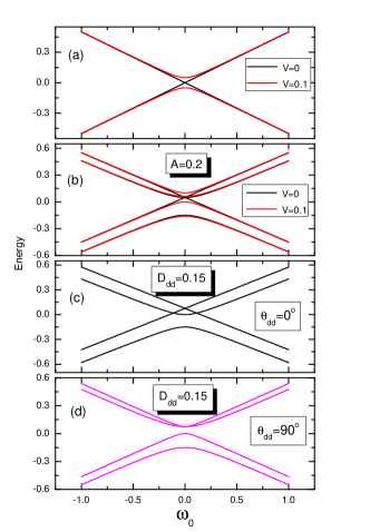
Figure 1: Energy levels of a single-spin (a) and two-spin (b–d) model systems. (a) Energy levels of the spin in the magnetic field directed along the $z$-axis in the absence of an external perturbation ($V=0$) and in its presence ($V=0.1$). (b) Energy levels of an electron-nuclear spin system coupled by isotropic HFC with $A=0.2$ assuming $V=0$ and $V=0.1$. Energy levels of an electron-nuclear spin system coupled by dipolar HFC assuming (c) $\bm{n}~{}||~{}z$ ($\theta_{dd}=0$) and (d) $\bm{n}\perp z$ ($\theta_{dd}=90^{o}$). In subplots (c, d) we have taken $A=V=0$.

Here we also extend the treatment to electron-nuclear spin systems, i.e., we consider interaction of the electron spin with surrounding nuclear spins by hyperfine coupling (HFC). For the sake of simplicity, we reduce the nuclear spin subsystem to only one spin $I=1/2$. Then the Hamiltonian of the spin system under consideration takes the form (in $\hbar$ units):

$$\hat{H}(t)=\omega_{0}\hat{S}_{z}+V\hat{S}_{x}+A(\hat{\bm{S}}\cdot\hat{\bm{I}})+\Omega_{1}\cos(2\pi f_{m}t)\hat{S}_{z},$$ (4)

where $\hat{\bm{I}}$ is the spin operator of the nucleus, $A$ is the isotropic HFC constant. The energy levels of a two-spin system are shown in Fig. 1b taking account for the isotropic HFC and the $V$-term. Additionally, we consider a model where dipolar HFC is used instead of isotropic HFC:

$$\hat{H}(t)=\omega_{0}\hat{S}_{z}+D_{dd}[3(\hat{\bm{S}},\bm{n})(\hat{\bm{I}},\bm{n})-(\hat{\bm{S}},\hat{\bm{I}})]+$$

$$+\Omega_{1}\cos(2\pi f_{m}t)\hat{S}_{z},$$ (5)

where $D_{dd}$ is the dipolar interaction strength depending on the distance between the spins and $\bm{n}$ is the vector pointing from one spin to the other with unity length, $|\bm{n}|=1$. In Fig. 1c,d we show the energy levels of such a system for different directions of $\bm{n}$. Here $\theta_{dd}$ is the angle between $\bm{n}$ and the $z$-axis, which is parallel to the external magnetic field. Hereafter, for the sake of simplicity, all parameters of the spin Hamiltonian as well as spin relaxation parameters are given in dimensionless units.

In our model, the observable signal is given by the population of one of the states of the $S$-spin, for clarity, the bright state is the $\alpha$-state. To make comparison with the experiments we multiply the population of the $\alpha$-state, $\rho_{\alpha\alpha}$, by the $\cos(2\pi f_{m}t)$ function and integrate it over the modulation period, see below.

Qualitatively, we expect different regimes for spin dynamics at $f_{m}\ll V$ and $f_{m}\gg V$ as demonstrated in Fig. 2 for a two-level system. At $f_{m}\ll V$ each passage through the LAC results in adiabatic inversion of populations of the $S$-spin states. Consequently, the luminescence signal is expected to be modulated at the $f_{m}$ frequency having the maximal possible amplitude and the same phase as the modulated external field. During a fast passage through the LAC, i.e., at $f_{m}\gg V$, the populations are mixed only slightly in each passage and the amplitude and frequency of modulation of the luminescence signal is expected to drop down. In addition, modulation of the signal is no longer in-phase with the reference signal of the lock-in amplifier, resulting in both considerable phase shifts and reduction of the signal. As we show below, the calculation results are in good agreement with this simple consideration.

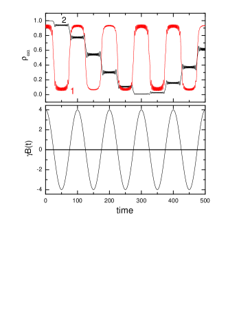
Figure 2: Spin dynamics resulting from passage through the LAC in a two-level system described by the Hamiltonian $\hat{H}(t)$ given by eq. (3). Top: population of the $\alpha$-state for adiabatic (curve 1) and non-adiabatic (curve 2) variation of the Hamiltonian. Bottom: magnetic field $\gamma B(t)=\Omega_{1}\cos(2\pi f_{m}t)$. Calculation parameters: $\omega_{0}=0$, $\Omega_{1}=4$, $f_{m}=0.01$, $V=1$ (curve 1) and 0.1 (curve 2); at $t=0$ the system is in the “bright” state; relaxation effects are neglected.

For systematic analysis we also take spin relaxation into account. To do so, we treat the spin evolution as described by the Liouville-von Neumann equation:

$$\frac{d\rho_{ij}}{dt}=L_{ij;kl}(t)\rho_{kl},$$ (6)

where $\rho$ is the density matrix of the two-spin electron-nuclear system in the Liouville representation (column vector with 16 elements), while the elements of the $\hat{\hat{L}}$ super-operator are as follows:

$$L_{ij;kl}=i(\delta_{ik}H_{lj}-\delta_{jl}H_{ik})+R_{ij;kl},$$ (7)

where $R_{ij;kl}$ is the relaxation matrix. To specify the $R$ super-operator we make the following simplifying assumptions. We treat two contributions to the electron spin relaxation, the longitudinal relaxation (relaxation of populations having the rate $R_{1}$) and transverse relaxation (relaxation of coherences having the rate $R_{2}$). We consider two different cases: $R_{1}=R_{2}$ and $R_{1}\ll R_{2}$, see below. In addition, we take into account photo-excitation of the NV^- center, which produces the electron spin polarization, i.e., the population difference for the states of the $S$-spin. This process is considered in a simplified manner as a transition from the $\beta$-state to the $\alpha$-state at a rate $J$ (pumping rate for the electron spin polarization). Thus, for the sake of simplicity, we do not consider the complete excitation cycle in the NV^- center, which gives rise to the electron spin polarization. Relaxation of the nuclear spin is completely neglected because it is usually much slower than that for the electron spin.

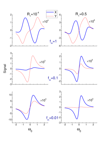
Figure 3: Theoretical LAC-spectra of a single-spin system for three different $f_{m}$ frequencies equal to 1 (top), 0.1 (middle) and 0.01 (bottom) and longitudinal relaxation rate $R_{1}$ equal to $10^{-4}$ (left) and $0.5$ (right). Here both components of the signal, $X$ (thick lines) and $Y$ (thin lines), are shown, calculated according to eqs. (10) and (11), respectively. Other calculation parameters are: $R_{2}=0.5$, $J=0.01$, $V=0.1$, $\Omega_{1}=0.1$.

To perform numerical calculations we split the modulation period $T=1/f_{m}$ into $N$ equal intervals of a duration $\Delta t=T/N$. In each step, the density matrix $\rho$ was propagated by using a matrix exponent:

$$\rho(t+\Delta t)=\exp[\hat{\hat{L}}(t)\Delta t]\rho(t).$$ (8)

Generally, the solution depends on the initial conditions. However, in the present case we are interested in the “steady-state” solution, which is reached after many modulation periods. Indeed, in experiments transient effects are not important because signal averaging is performed over many $T$ periods (only the steady-state of the system is probed). To obtain such a solution of eq. (6) we assume that the density matrix before a period of modulation, $\rho(0)$, is the same as that after the period:

$$\rho(0)=\rho(T) = \exp[\hat{\hat{L}}(t=T-\Delta t)\Delta t]\times\ldots$$

$$\times\exp[\hat{\hat{L}}(t=0)\Delta t]\rho(0)=\hat{\hat{U}}\rho(0).$$ (9)

Here $\hat{\hat{U}}$ is the super-matrix, which describes the evolution over a single modulation period. This equation is a linear equation for the $\rho(0)$ vector. To find a non-trivial solution of such a matrix equation, we need to exclude one equation from the system (the one, which linearly depends on other equations) and to replace it by the expression $\sum_{i}\rho_{ii}(0)=1$, which describes nothing else but conservation of the trace of the density matrix. This new system can be solved by using linear algebra methods. The $\hat{\hat{U}}$ matrix is computed numerically; to do so we set the value of $N$ such that further increase of $N$ changed the final result by less than 1%. Of course, it is necessary to increase $N$ substantially at small $f_{m}$. At the lowest modulation frequency we typically use $N=2\times 10^{6}$.

To compare theoretical results to the experimental data we numerically compute the sine and cosine Fourier components of the element of interest of the density matrix, namely, the population of the $\alpha$-state, $\rho_{\alpha\alpha}$. This element can be computed when $\rho(t)$ is known:

$$X=\frac{1}{T}\int_{0}^{T}\rho_{\alpha\alpha}\cos(2\pi f_{m}t)dt,$$ (10)

$$Y=\frac{1}{T}\int_{0}^{T}\rho_{\alpha\alpha}\sin(2\pi f_{m}t)dt.$$ (11)

Knowing $X$ and $Y$ we can completely characterize the signal. An analogue of the lock-in detector phase variation by an angle $\phi$ is the rotation of axes in the functional space:

$$X^{\prime}=X\cos\phi+Y\sin\phi.$$ (12)

Typical calculated LAC-spectra are presented in Fig. 3 for three different $f_{m}$ frequencies; both components of the signal, $X$ and $Y$, are shown. Calculation of the two signal components is performed using eqs. (10) and (11). When the modulation frequency is low and relaxation of populations is relatively fast the $X$-component of the signal is strong whereas the $Y$-component is negligible, i.e., the signal is cosine-modulated and there is virtually no phase shift with respect to the modulated input signal $\Omega_{1}\cos(2\pi f_{m}t)$. At higher modulation frequency both components of the signal are significant, i.e., there is a strong phase shift with respect to the input signal. The appearance of the spectra changes upon variation of the $R_{1}$ rate. Upon decrease of the $f_{m}$ frequency not only the $Y$-component is reduced but also the signal intensity grows. As we demonstrate below, such a behavior of the LAC-lines is consistent with experimental findings.

III Results and Discussion

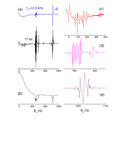
Figure 4: Experimental LAC spectra of NV^- centers in a diamond single crystal. (a) LAC spectra in the range $-50$-$1200$ G obtained using the modulation frequency $f_{m}$ of 12.5 kHz and 17 Hz; the upper trace is multiplied by 5. (b) Integrated LAC spectrum obtained with $f_{m}=17$ Hz. Subplots (c), (d) and (e) show enlarged different regions of the LAC spectrum. In all cases the modulation amplitude was $\Omega_{1}=0.5$ G. Except for the upper trace in (a) the modulation frequency was 17 Hz. The lock-in detector phase was chosen such that the LAC-line at 1024 G has maximal amplitude.

III.1 Experimental LAC-spectra

In Fig. 4 we show the transformation of the LAC-spectra upon variation of the modulation frequency. In subplot (a) we show the results for two different frequencies, 12.5 kHz and 17 Hz. One can readily see that the amplitude of all lines is much higher at the low $f_{m}$ value. For better presentation we compare the original spectra with integrated LAC spectra: in the integrated spectra all LAC-lines show up as dips in the $B_{0}$ dependence. One can readily see that LAC-lines are much better visible in the spectra obtained with field modulation. LAC-lines that show up only at low modulation frequency are analyzed in our previous work Anishchik et al. (2016) and originate from polarization transfer between paramagnetic defect centers. Here we only briefly mention the main peculiarities of the detected LAC-lines, see Fig. 4c,d,e. Polarization transfer between defect centers occurs when the level splittings in the two centers become equal to each other (causing a level crossing): under such conditions electronic dipole-dipole interaction turns a level crossing into an LAC and enables coherent polarization exchange. Such a polarization transfer is usually termed (perhaps, erroneously because polarization transfer is due to a coherent mechanism) cross-relaxation van Oort and Glasbeek (1989).

The line at zero fieldAnishchik et al. (2015) comes from polarization transfer between two NV^- centers; for symmetry reasons at zero field energy matching for two NV^- centers always occurs, consequently, the zero-field line has been found in all samples we studied so far. Other lines emerging in the field range 50–400 G, which are visible only at low modulation frequencies, are due to interaction of the NV^- center with other paramagnetic defect centers in the crystal; quantitative analysis of the positions and amplitudes of these lines thus provides valuable information about the Electron Paramagnetic Resonance (EPR) parameters (spin value, zero-field splitting, hyperfine couplings) of these centers. The LAC-lines found around 500 G and at 590 G become considerably stronger at $f_{m}=17$ Hz; the former are coming from interaction of the NV^- center with the P1-center (neutral nitrogen atom, replacing carbon in the diamond lattice) while the latter comes from interaction of two NV^- centers having different orientations with respect to the external magnetic field. Additionally, the line at 1024 G corresponds to the LAC in the NV^- in its ground state. Finally, the satellite lines at 1007 G and 1037 G are seen in the LAC-spectrum. These lines are originating from polarization exchange between the spin-polarized NV^- center and the P1-centerArmstrong et al. (2010). The low amplitude of the satellite lines is due to the weak interaction between different defect centers.

Hence, one can see that the amplitude of all LAC-lines is very sensitive to the $f_{m}$ value, so that some lines can be found only using very low modulation frequency. For this reason, we find it important to analyze the $f_{m}$ dependence of LAC-lines and elucidate the parameters that determine this dependence.

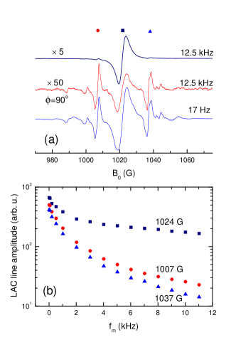
Figure 5: (a) Experimental LAC spectra of NV^- centers in a diamond single crystal in the magnetic field range 970-1075 G. For each curve the $f_{m}$ value used in experiments is specified. For the upper curve the phase of the lock-in detector is chosen such that the signal for the central LAC-line is maximal. For the middle trace the phase is shifted by $90^{\circ}$ with respect to that for the upper curve. The amplitude of the upper curve is increased by a factor of 5, for the middle curve – by a factor of 50. The LAC-lines are indicated by circle, square and triangle. (b) $f_{m}$ dependence of the amplitude of the three LAC-lines (symbols correspond to the LAC-lines in subplot a). For each curve the magnetic field strength $B_{0}$ corresponding to the center of the corresponding line is specified. For each experimental point the lock-in detector phase is set such that the amplitude of the corresponding line was maximal. In all cases the modulation amplitude was $B_{m}=0.5$ G.

Fig. 5a shows the LAC-spectra of the NV^- center in the field range 970-1075 G. The spectra shown for two different modulation frequencies, 12.5 kHz and 17 Hz, are remarkably different. As it is seen from the Figure, when $f_{m}=12.5$ kHz and the lock-in detector phase is set such that the central line at 1024 G has the maximal amplitude, the satellite lines at 1007 G and 1037 G are barely visible. When the modulation frequency is reduced to 17 Hz the amplitude of the central line increases by a factor of 7, whereas the satellite lines become 50 times stronger. Additionally, at low frequency the phase shift for all lines is negligible in contrast to that at the high modulation frequency. As it is seen from the LAC-spectrum there are no new lines appearing in the spectrum in this field range but the signal-to-noise ratio is substantially increased.

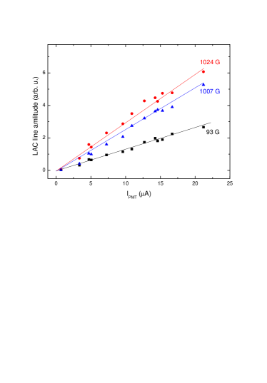
Figure 6: Dependence of the LAC-line at 95 G, 1007 G and 1024 G amplitudes on the luminescence intensity of the sample, which is proportional to the current, $I_{PMT}$, in the photo-multiplier. The modulation frequency $f_{m}$ is 17 Hz; the modulation amplitude is 0.5 G.

In Fig. 5b we present the experimental dependence of the line amplitudes, as determined for the three different LAC-lines, on the modulation frequency. Here the total peak-to-peak amplitude is presented; the lock-in detector phase is set such that for each experiment the amplitude of the corresponding line is maximal. It is clearly seen that by varying the modulation frequency we obtain a strong variation of the LAC-line amplitudes, by roughly two orders of magnitude. In the frequency range under study the dependence is concave, i.e., the slope of the curve increases at lower modulation frequencies. Hence, by using modulation we not only obtain the “derivative” spectrum: modulation strongly affects the line amplitudes and shapes. We attribute this dependence to the spin dynamics caused by modulation. The most unexpected effect is that the increase of the line amplitude is occurring at modulation frequencies, which are much smaller than the electron spin phase relaxation rates of the NV^- center (when measured in the same units). In samples like the one we use the phase relaxation times are typically about several microseconds Kennedy et al. (2003); Rondin et al. (2014). Our estimates for the phase relaxation times (as determined from the widths of the EPR and optically detected magnetic resonance spectra) in our samples agree with these values. Such relaxation times correspond to the frequencies of the order of several 100 kHz to several MHz. For this reason the growth of the LAC-line amplitude upon the decrease of $f_{m}$ from some 10 kHz to several Hz (in particular, the sharp increase of the line amplitude at very low frequencies) is perplexing.

In Fig. 6 we show the experimental dependence of the LAC-line amplitudes on the luminescence intensity of the studied sample (the current of the photo-multiplier is proportional to this intensity). Since the luminescence intensity is directly proportional to the intensity of the excitation light these data present the dependence of the LAC-line amplitudes on the intensity of incident light. One can clearly see that the dependence is almost perfectly linear (in contrast to the quadratic dependence reported for the zero-field LAC-line Anishchik et al. (2015)). Hence, the increase of the LAC-line amplitude at low $f_{m}$ frequencies cannot be attributed to any two-photon processes.

III.2 Theoretical calculations

To rationalize the behavior of the LAC-lines upon variation of $f_{m}$ we perform simulations of the spin dynamics of single-spin and two-spin systems at LACs. Simulations for the single $S$-spin model properly reproduce the $f_{m}$-dependence at high frequencies: the signal decays roughly as $1/f_{m}^{2}$. Assuming $R_{1}=R_{2}$ we are not able to reproduce the experimental dependence: at low $f_{m}$ the theoretical curve flattens and the line amplitude does not increase further.

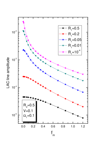
Figure 7: Calculated amplitude of the LAC-line (peak-to-peak) for the single $S$-spin model as a function of $f_{m}$. The calculation parameters are given in the graph.

The experimentally observed growth at low frequency is clearly an indication of a slow dynamic process in the system. We attribute this process to $T_{1}$-relaxation (longitudinal relaxation): in solids $T_{1}$-relaxation is usually much slower than $T_{2}$-relaxation, i.e., $R_{1}\ll R_{2}$. This is correct for the NV^- centers in diamond as wellJarmola et al. (2012, 2015). Under the assumption $R_{1}\ll R_{2}$ we obtain an $f_{m}$-dependence, which is much closer to the experimental one: while the behavior at high $f_{m}$ remains the same, the LAC-line amplitude continues to grow at low frequency. It is worth noting that in the logarithmic-linear coordinates at small $R_{1}$ the $f_{m}$ dependence has the same shape (concave shape, i.e., the second derivative of the curve is positive; there is an inflexion point at low $f_{m}$) as the experimentally observed dependence. However, such a model predicts a smaller effect of $f_{m}$ than that found experimentally. Specifically, at small $f_{m}$ the calculated curve levels off (the slope of the curve tends to zero at $f_{m}\to 0$).

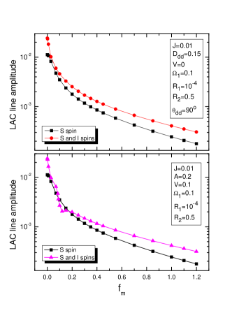
Figure 8: Calculated amplitude of the LAC-line (peak-to-peak) for the electron-nuclear two-spin system as a function of $f_{m}$. In the upper graph we present the calculation result for dipolar HFC and in the lower graph - for isotropic HFC. The calculation parameters are given in the graph.

The observed strong $f_{m}$ dependence can be explained by polarization transfer from the electronic spin system to nuclear spins having even longer relaxation times than $T_{1}$. The calculation performed for the electron-nuclear spin system confirms this expectation: while at high $f_{m}$ frequencies the calculation result is almost the same for the single-spin system and two-spin system, at low $f_{m}$ values a sharper increase of the LAC-line amplitude is found for the electron-nuclear spin system. We attribute this sharper increase to the effect of the long nuclear $T_{1}$-relaxation time.

In Fig. 8 we present the calculated $f_{m}$ dependence of the LAC-line amplitude for the electron-nuclear spin system assuming dipolar (upper graph) and isotropic (upper graph) HFC and compare it to the same dependence for the two-level system. One can see that in the two-spin system the LAC-line continues to grow even at low $f_{m}$; this is due to polarization transfer between the electron and nucleus. The only difference between the two cases, dipolar vs. isotropic HFC, is that the curve is monotonous for the dipolar HFC (similar to the experimental observation), whereas for the isotropic HFC there is a feature seen at $f_{m}$ close to the $A$ value. It is also worth noting that assuming isotropic HFC we can obtain the LAC-line only when $V\neq 0$ while for the dipolar HFC the LAC-line amplitude is non-zero even when $V=0$ (except for the case $\bm{n}~{}||~{}z$).

IV Conclusions

We report a study of LAC-lines in the NV^- defect centers in diamond crystals by using lock-in detection of the signal. Such a method allows one to obtain sharp LAC-lines with excellent signal-to-noise ratio. A strong and unexpected effect of the modulation frequency on the LAC-line amplitude is demonstrated. Importantly, the LAC-lines are the strongest at low modulation frequencies. Thus, measurements at low $f_{m}$ are advantageous, even despite the technical issues concerning experiments at low frequencies (namely, the instrumental noise). Moreover, LAC-spectra obtained at low modulation frequencies are free from distortions and phase shifts of the signal with respect to the reference signal of the lock-in amplifier.

To rationalize the observed effect of the modulation frequency we performed a theoretical study and computed numerically the evolution of the spin system under the action of the modulation field. In the theoretical model, we introduced a single electron spin 1/2 (modeling the electron spin degrees of freedom of the NV^- center) coupled to a nuclear spin 1/2. Such a model can reproduce the main features found in experiments suggesting that field modulation strongly modifies the dynamics of the spin system at LACs. Specifically, at low modulation frequency we obtained adiabatic exchange of populations of the states having an LAC, whereas non-adiabatic population exchange at high $f_{m}$ values leads to decrease of the LAC-line amplitude accompanied by the phase shift. In order to reproduce the further increase of the LAC-line amplitude at low $f_{m}$ frequencies we considered slow dynamic processes, such as electronic $T_{1}$-relaxation (which is, in solids, commonly much slower than $T_{2}$-relaxation) and nuclear spin relaxation. Account of these relaxation processes allowed us to reproduce the experimentally observed $f_{m}$ dependences.

Our work provides useful practical recommendations on how to conduct experimental studies of LAC-lines. As we show in a subsequent publication, the experimental method used here indeed enables sensitive detection of LAC-lines. Furthermore, for the first time we demonstrate that modulation (used in lock-in detection) is not only a prerequisite for sensitive detection of weak signals but also a method to affect spin dynamics of the NV^- centers in diamonds. Last but not least, our experimental method allows one to detect new LAC-lines. Such LAC-lines can be used for indirect detection of otherwise “invisible” paramagnetic defect centers in diamond crystals; their analysis has been in part performed in Ref. Anishchik et al. (2016). A more detailed analysis will be elsewhere.