Laplace-transformed multi-reference second-order perturbation theories in the atomic and active molecular orbital basis

Abstract

In the present article, we show how to formulate the partially contracted n-electron valence second order perturbation theory (NEVPT2) energies in the atomic and active molecular orbital basis by employing the Laplace transformation of orbital-energy denominators (OED). As atomic-orbital (AO) basis functions are inherently localized and the number of active orbitals is comparatively small, our formulation is particularly suited for a linearly-scaling NEVPT2 implementation. Some of the NEVPT2 energy contributions can be formulated completely in the AO basis as single-reference second-order Møller–Plesset perturbation theory and benefit from sparse active-pseudo density matrices — particularly if the active molecular orbitals are localized only in parts of a molecule. Furthermore, we show that for multi-reference perturbation theories it is particularly challenging to find optimal parameters of the numerical Laplace transformation as the fit range may vary among the 8 different OEDs by many orders of magnitude. Selecting the number of quadrature points for each OED separately according to an accuracy-based criterion allows us to control the errors in the NEVPT2 energies reliably.

I Introduction

Many applications of quantum chemical simulations require a multi-reference (MR) wave function to provide an at least qualitatively correct description of the atomic or molecular system. Even the simplest molecule — the hydrogen molecule — becomes a MR case in the process of separating the two hydrogen atoms. MR theories are also indispensable when two potential energy surfaces of the same symmetry come close in energy, which is frequently encountered when studying the time evolution of excited electrons in molecules — in particular by surface-hopping excited-state dynamics.Martínez (2006); *Subotnik2016 Beyond a reliable treatment of bond breaking and potential energy surfaces, MR theories are often considered in quantum chemical studies that involve transition metals, lanthanides, and actinides to cope with open shells in the electronic structure calculation. Alternatively, Kohn-Sham density functional theory (DFT) can often provide meaningful energies and properties for transition metal complexes with low computational costs even when standard exchange correlation functionals are employed. However, DFT still lacks an ansatz that can improve systematically on either static or dynamic correlation effects in a computationally affordable manner.

In comparison to their single-reference (SR) analogues, wave function-based MR electronic structure methods are conceptually and computationally much more demanding. At the multi-configurational (MC) self-consistent field (SCF) level, the energy needs to be minimized with respect to orbital rotations and configuration coefficients, which in many situations requires sophisticated optimizers with quadraticLengsfield (1980) or higherWerner and Meyer (1980); *Werner1981; *Werner1985 convergence rates. On the one hand, such algorithms can be incredibly efficient in terms of number of iterations; on the other hand, a transformation of the two-electron integrals from the atomic (AO) to the molecular orbital (MO) basis is necessary, which scales $\mathcal{O}(N^{5})$ with the system size $N$. Moreover, the MCSCF wave function is expanded in configuration state functions (CSF) that can be generated by a complete active spaceRoos, Taylor, and Siegbahn (1980) (CAS). The latter includes all possible occupations of $N_{\text{act}}$ active MOs by $N_{\text{el}}$ active electrons usually denoted by CAS ($N_{\text{el}}$,$N_{\text{act}}$). With conventional determinant-based full configuration interaction (FCI) implementationsKnowles and Handy (1984); Olsen, Jørgensen, and Simons (1990) the computational costs grow exponentially and becomes soon a bottleneck in the MCSCF calculation. Usually, one is restricted to active spaces in the ballpark of a CAS (10,30) if no restrictedOlsen et al. (1988) (RAS) or generalized active spacesFleig, Olsen, and Marian (2001) (GAS) are desired.

There are recent developments in MCSCF that improve on both computational bottlenecks of the algorithms: the two-electron integral transformation and the size limit of the active space. The latter can be lifted if the CAS CI secular equations are solved by modern quantum Monte CarloBooth, Thom, and Alavi (2009); Thomas et al. (2015) or density matrix renormalization groupWhite (1992); *whit93 (DMRG) algorithms. This facilitates CASSCF calculations with much larger active spaces, e. g. $N_{\text{el}}\times N_{\text{act}}\approx 2000$.Zgid and Nooijen (2008a); *zgid08b; *ghos08; *yana09a; *kurashige2011; *wouters2014; *wout15; *mayi16c; *LiManni2016; Knecht et al. (2016); Sun, Yang, and Chan (2017) As shown lately by Hohenstein et al.Hohenstein et al. (2015)  for an approximate second-order optimizerChaban, Schmidt, and Gordon (1997), the costly integral transformations can be avoided by initially computing Coulomb- and exchange-like matrices in the sparse AO basis with $\mathcal{O}(N^{2})$ costs and later transforming to Fock-like intermediates and orbital gradients in the MO basis. Just recently, a truly second-order optimizer that is also AO-driven and can handle a large number of AOs and active MOs was proposed in Ref. 26

The computationally simplest approach to account for dynamic correlation in molecules that demand for multiple reference determinants is second-order multi-reference perturbation theory (MRPT2). MRPT2 methods made substantial progress over the last 25 years and are frequently used in quantum chemical investigations. In particular, the CASPT2 methodAndersson et al. (1990); *Andersson1992 initially developed by Andersson et al. has evolved into a reliable tool for the investiagation of molecules with a complicated electronic structure. Geometries can be conveniently optimized due to availability of analytic CASPT2 gradients,Celani and Werner (2003); *Shiozaki2011; *Gyoerffy2013 which were developed by Werner and his co-workers. Accurate CASPT2 energies and gradients near the complete basis set limit can be obtained with an explicitly correlated F12 variant proposed by Shiozaki et al.Shiozaki and Werner (2010); *Shiozaki2013 For calculations involving heavy elements, spin-orbit coupling (SOC) can be treated either within a SOC-CI formalismRoos and Malmqvist (2004) or by using the four-component Dirac-Coulomb Hamiltonian.Abe, Nakajima, and Hirao (2006) Concerning studies of excited states, the erratic mixing of valence and Rydberg states at the CASSCF level can be cured by using quasi-degenerate MRPT2.Finley et al. (1998); Angeli et al. (2004)

Despite its popularity and success in numerous application, CASPT2 has two major drawbacks: (i) It is not size-consistent; (ii) It is often plagued by intruder states, which complicates the iterative determination of the first-order wavefunction coefficients. In practice, the size-inconsistency errors are rather decent — even for larger moleculesMenezes, Kats, and Werner (2016) — and the intruder-state problem can be cured partially by level shifts.Roos and Andersson (1995); *Forsberg1997 However, since level shifts alter the second-order energy unpredictably, CASPT2 should then be considered as a rather empirical method.

The remedies of CASPT2 are cured altogether within a different formulation of MRPT: the n-electron valence (NEV) PT of Angeli, Cimiraglia, Malrieu and their co-workers.Angeli, Cimiraglia, and Malrieu (2000); Angeli et al. (2001); Angeli, Cimiraglia, and Malrieu (2001, 2002) NEVPT2 differs from CASPT2 mainly in the definition in the zeroth-order Hamiltonian. In NEVPT the Fock operator is replaced by the Dyall HamiltonianDyall (1995), which also accounts for explicit two-electron interactions within the active orbitals. Initially, two variants of NEVPT were introduced that differ in the level of so-called outer-space contraction:Angeli et al. (2001) the partially contracted (PC) and strongly contracted (SC) NEVPT2. Both variants are fully internally contracted (IC) and require the computation of the four-particle reduced density matrix (RDM), which scales with $\mathcal{O}(N_{\text{act}}^{8})$. With the rise of DMRG and FCIQMC algorithms in the last two decades, relatively large active spaces are now feasible for CASSCF, but become prohibitive in the subsequent IC-MRPT calculation. A rigorous approach to this dilemma would be to use completely uncontracted first-order wavefunctions, which was initially considered as computationally not feasible. Recent developmentsSharma and Chan (2014); Sokolov and Chan (2016); Giner et al. (2017) reveal, however, the clear potential of fully uncontracted MRPT for calculations that demand large active spaces.

Most systems with MR character that have a practical relevance, e. g. metal-organic complexes, enzymes, or organic radicals, have a rather small number of active orbitals compared to the total number of MOs. In such situations, the computational costs of MRPT2 are dominated by the $\mathcal{O}(N^{5})$ scaling integral transformations as for SR second-order Møller–Plesset PT (MP2). A substantial reduction of the timings can be achieved by employing a CD of two-electron integralsAquilante et al. (2008); *Freitag2017, in particular, if such an integral decomposition technique is combined with a truncated or frozen natural orbital (FNO) virtuals basis.Aquilante et al. (2009) However, for FNO- or CD-MRPT2 only the pre-factor of the computational costs is reduced but the scaling is still $\mathcal{O}(N^{5})$ as for conventional implementations. Thus, calculation that exploit those approximations are still limited to medium-sized molecules in the ballpark of 100 atoms. Much larger systems can be calculated if the first-order wave function is expanded in a truncated set of pair natural orbitals (PNO), which was explored recently by the NeeseGuo et al. (2016) and Werner groupsMenezes, Kats, and Werner (2016) for PNO-NEVPT2 and PNO-CASPT2, respectively. Both implementations scale linearly with the system size and allow to perform MRPT2 calculations of molecules with up to 300 atoms.

In the present article, we pursue an alternative approach to reach linearly scaling MRPT2 implementations eventually. It is based on the Laplace transformation of orbital-energy denominators,Almlöf (1991) which was introduced initially by Almlöf in the context of MP PT.Häser and Almlöf (1992); Häser (1993) In our formulation, all intermediates are given solely in the AO and active MO basis, which is in line with recent algorithmic developments in MCSCFHohenstein et al. (2015); Sun, Yang, and Chan (2017). On the one hand, the number of active MOs $N_{\text{act}}$ can still be considered as small in MR calculations because even with modern DMRG and FCIQMC implementations solving the CAS CI secular equations may easily become a computational bottleneck due to the formal exponential cost scaling with $N_{\text{act}}$. On the other hand, localized AO basis functions are inherently suited for effective screening. It was shown by Ayala and ScuseriaAyala and Scuseria (1999) that SR Laplace-transformed AO-MP2 energies show the physically correct $R^{-6}$ decay with the distance $R$ between charge distributions. This was exploited later by Ochsenfeld and his co-workers,Lambrecht, Doser, and Ochsenfeld (2005); Doser et al. (2009); *Maurer2013b who introduced integral estimates with the proper $R$ dependence to develop linearly scaling MP2 implementations. With those AO-based implementations MP2 calculations on molecules with more than 1000 atoms and more than 10000 basis functions were reported.Doser et al. (2009) However, since the initial AO-MP2 implementation of HäserHäser (1993), AO-based wave function methods were criticized for their large computational overhead that increases substantially for larger basis sets. This problems can be solved now by a Cholesky decomposition (CD) of (pseudo-)densitiesZienau et al. (2009), which leads to intermediates that have the same dimension as the occupied or virtual MO coefficients but retain the sparsity of AO (pseudo-)density matrices.Kussmann et al. (2015); Luenser, Schurkus, and Ochsenfeld An extension of Laplace-transformed AO-based MP2 for relativistic all-electron calculations was introduced recently by one of the present authors for two-component Hamiltonians and the Kramers-restricted formalism.Helmich-Paris, Repisky, and Visscher (2016)

In this work, we show how to formulate NEVPT2 in the atomic and active molecular orbital basis by means of the numerical Laplace transformation. We start in Sec. II with a résúme of present state-of-the-art IC-MRPT2 theories and argue why only the partially-contracted NEVPT2 is suitable for such a re-formulation. Moreover, we outline how to obtain PC-NEVPT2 energies in the AO and active MO basis in the spin-free formalism and provide working equations for each energy contribution. In Sec. IV, the working equations are discussed in context of a potentially efficient implementation. Furthermore, we focus on how to control the error of the numerical quadrature of the Laplace transformation for each of the individual energy contributions. Finally, our procedure is validated for some typical applications of MRPT methods that involve bond dissociation and excited valence and Rydberg states.

II Theory

II.1 Résúme of CASPT2 and NEVPT2

The zeroth-order wavefunction is given by a linear combination

$$|0\rangle\equiv|\Psi^{(0)}\rangle=\sum_{K}c_{K}|K\rangle$$ (1)

of all configuration state functions $|K\rangle$. The wavefunction parameters, that is orbital rotations and CI coefficients $c_{K}$, can be optimized either in a MCSCF or open-shell HF and subsequent CI calculation. The first-order correction to the wave function

$$|\Psi^{(1)}\rangle=\sum_{\mu_{2}}C_{\mu_{2}}|\Phi_{\mu_{2}}\rangle=\sum_{\mu_{2}}C_{\mu_{2}}\hat{\tau}_{\mu_{2}}|0\rangle$$ (2)

is expanded through all possible determinants that are generated by two-electron excitations from the complete zeroth-order wavefunction. This approximation is termed internal contraction (IC) and $|\Phi_{\mu_{2}}\rangle$ is referred to as internally contracted configurationsCelani and Werner (2000) (ICC). To determine the PT energy through second order,

$$E^{(2)}=\langle 0|\hat{H}|\Psi^{(1)}\rangle=\langle 0|\hat{H}\hat{\tau}_{\mu_{2}}|0\rangle C^{(1)}_{\mu_{2}}\text{,}$$ (3)

the expansion coefficients of the first-order wave function $C^{(1)}_{\mu_{2}}$ are determined by solving the linear system of equations

$$\langle\widetilde{\Phi_{\mu_{2}}}|\hat{H}^{(0)}-E^{(0)}|\Psi^{(1)}\rangle =\sum_{\nu_{2}}\langle\widetilde{\Phi_{\mu_{2}}}|[\hat{H}^{(0)},\hat{\tau}_{\nu_{2}}]|0\rangle C_{\nu_{2}}$$

$$=-\langle\widetilde{\Phi_{\mu_{2}}}|\hat{H}|0\rangle\text{.}$$ (4)

In Eq. (II.1) we assume that diagonalization of the zeroth-order Hamiltonian,

$$\hat{H}^{(0)}|0\rangle=E^{(0)}|0\rangle\text{,}$$ (5)

gives the MCSCF or CI eigenvalues $E^{(0)}$ and zeroth-order wave function $|\Psi^{(0)}\rangle$. As projection manifold $\{\langle\widetilde{\Phi_{\mu_{2}}}|\}$ we choose bra ICCs in Eq. (II.1) such that they keep the core and virtual part of the ICC overlaps $\langle\widetilde{\Phi_{\mu_{2}}}|\Phi_{\nu_{2}}\rangle$ orthogonalPulay, Sæbø, and Meyer (1984); *Helgaker2000-biortho because simplified arithmetic expressions are obtained.

To build $|\Psi^{(1)}\rangle$, the mutually orthogonal ICCs are generated by exciting two electrons out of the core or active into the virtual or active molecular orbitals (MO) of the zeroth-order wavefunction $|\Psi^{(0)}\rangle$. There are 8 different classes of ICCs if the reference determinants $|K\rangle$ were built from a complete active space (CAS), which are compiled in Tab. 3. In the present work, we use spin-free operators that are composed of singlet one-particle excitation operators

$$\hat{E}_{pq}=\sum_{\sigma}\hat{a}^{{\dagger}}_{p\sigma}\hat{a}_{q\sigma}\,\text{,}\quad\sigma=\{\alpha,\beta\}$$ (6)

We follow the convention that core orbitals are denoted by $i,j,k,l$, active orbitals by $t,u,v,w$, virtual orbitals by $a,b,c,d$, and general orbitals by $p,q,r,s$. The different classes of ICCs in Tab. 3 are labeled by symbols that became standard notation in NEVPT: $+n$ denotes attachment of $n$ electron(s) into the active space while $-n$ means ionization of $n$ electron(s) from the active space; a prime designates a single-particle excitation within the active orbital space. In contrast to other ICCs, the one of the $\left[0\right]^{\prime}$ class are composed of two kinds of excited determinants, $|\Phi_{it}^{au}\rangle$ and $|\Phi_{it}^{ua}\rangle$, that are mutually non-orthogonal. If RAS or GAS were employed in the underlying MCSCF calculation, the expansion of $|\Psi^{(1)}\rangle$ in terms of ICCs needs to be augmented with a subset of the CAS space determinants, i. e. $|\Phi_{tv}^{uw}\rangle=\hat{E}_{ut}\hat{E}_{wv}|0\rangle$, to keep the zeroth- $|\Psi^{(0)}\rangle$ and first-order wavefunction $|\Psi^{(1)}\rangle$ mutually orthogonal.Celani and Werner (2000) In the present work, we only consider CAS reference wavefunctions.

In MRPT the definition of the zeroth-order Hamiltonian $\hat{H}^{(0)}$ is not unique and it is the choice of $\hat{H}^{(0)}$ in which CASPT2 and PC-NEVPT2 mainly differ. In CASPT2 the zeroth-order Hamiltonian

$$\hat{H}^{(0)} =\hat{P}\hat{F}\hat{P}+\hat{Q}\hat{F}\hat{Q}$$ (7)

is defined by projection of the Fock operator

$$\hat{F} =\sum_{pq}f_{pq}\hat{E}_{pq}\text{,}$$ (8)

$$f_{pq} =f^{\text{I}}_{pq}+{{}^{A}}f_{pq}\text{,}$$ (9)

$$f^{\text{I}}_{pq} =h_{pq}+\sum_{i}\left[2(pq|ii)-(pi|iq)\right]\text{,}$$ (10)

$$f^{\text{A}}_{pq} =\frac{1}{2}\sum_{tu}\left[2(pq|tu)-(pu|tq)\right]\gamma_{tu}\text{,}$$ (11)

onto the space of reference determinants $\hat{P}=|0\rangle\langle 0|$ and its complement $\hat{Q}=\hat{1}-\hat{P}$.Celani and Werner (2000) The inactive $f^{\text{I}}_{pq}$ and active $f^{\text{A}}_{pq}$ Fock matrixHelgaker, Jørgensen, and Olsen (2000b) are built from the one- $h_{pq}$ and two-electron integrals $g_{pqrs}$, as they appear in the electronic Hamiltonian

$$\hat{H} =\sum_{pq}h_{pq}\hat{E}_{pq}+\frac{1}{2}\sum_{pqrs}g_{pqrs}(\hat{E}_{pq}\hat{E}_{rs}-\delta_{qr}\hat{E}_{ps})\text{,}$$ (12)

$$h_{pq} =\sum_{\mu\nu}C_{\mu p}C_{\nu q}h_{\mu\nu}\text{,}$$ (13)

$$g_{pqrs} \equiv(pq|rs)=\sum_{\mu\nu\kappa\lambda}C_{\mu p}C_{\nu q}C_{\kappa r}C_{\lambda s}(\mu\nu|\kappa\lambda)\text{,}$$ (14)

and the singlet one-particle reduced density matrix (1-RDM) $\gamma_{tu}$ (see Tab. 2). The integrals in the AO basis $h_{\mu\nu}$ and $(\mu\nu|\kappa\lambda)$ are transformed to the corresponding MO integrals $h_{pq}$ and $g_{pqrs}$ by MO coefficients $C_{\mu p}$ that are available from the preceding MCSCF or open-shell HF calculation. The CI coefficients appear only in the n-RDMs, as given in Tab. 2, for IC PTs, which are our focus here.

Due to the non-diagonal block structure of $\hat{Q}\hat{f}\hat{Q}$ in CASPT2, $\hat{H}^{(0)}$ can couple different classes of ICCs in $\langle\widetilde{\Phi_{\mu_{2}}}|[\hat{H}^{(0)},\hat{\tau}_{\nu_{2}}]|0\rangle$. This has two unpleasant implications: first, Eq. (II.1) must be determined iteratively and a larger computational overhead compared to a direct method like single-reference MP2 is expected; second, CASPT2 may not be size extensivevan Dam, van Lenthe, and Pulay (1998); *VanDam1999 what, in principle, disqualifies the method to be applied to large molecular systems. Furthermore, the usage of the Fock operator not only for core and virtual but also for the active orbitals may lead to (near) singularities in Eq. (II.1). In particular, ICC blocks in $\langle\widetilde{\Phi_{\mu_{2}}}|[\hat{H}^{(0)},\hat{\tau}_{\nu_{2}}]|0\rangle$ that involve three active orbitals, $[-1]^{\prime}$ and $[+1]^{\prime}$, are most likely to become zero.Dyall (1995); Angeli, Cimiraglia, and Malrieu (2000) This is the root of the notorious CASPT2 intruder state problem, which can be cured either by including more orbitals into the active space or in an empirical fashion by introducing level shifts in the zeroth-order HamiltonianRoos and Andersson (1995); *Forsberg1997. Furthermore, near singularities in $\langle\widetilde{\Phi_{\mu}}|[\hat{H}^{(0)},\hat{\tau}_{\nu}]|0\rangle$ would impede its Laplace transform as many quadrature points in the numerical integration procedure would be required then.

The NEVPT2 zeroth-order Hamiltonian features only diagonal ICC blocks,Dyall (1995)

$$\hat{H}^{(0)} =\hat{P}\hat{H}^{\text{D}}\hat{P}+\hat{P}^{\left[0\right]}\hat{H}^{\text{D}}\hat{P}^{\left[0\right]}+\ldots+\hat{P}^{\left[0\right]^{\prime}}\hat{H}^{\text{D}}\hat{P}^{\left[0\right]^{\prime}}\text{,}$$ (15)

which can guarantee size extensivity.van Dam, van Lenthe, and Pulay (1998); *VanDam1999 Furthermore, Dyall’s Hamiltonian $\hat{H}^{\text{D}}$ is employed in Eq. (15) that chooses the core $\hat{H}_{\text{c}}$ and valence part $\hat{H}_{\text{v}}$ differently,

$$\hat{H}^{\text{D}} =\hat{H}_{\text{c}}+\hat{H}_{\text{v}}+C\text{,}$$ (16)

$$\hat{H}_{\text{c}} =\sum_{ij}f_{ij}\hat{E}_{ij}+\sum_{ab}f_{ab}\hat{E}_{ab}\text{,}$$ (17)

$$\hat{H}_{\text{v}} =\sum_{tu}f^{\text{I}}_{tu}\hat{E}_{tu}+\frac{1}{2}\sum_{tuvw}(tu|vw)(\hat{E}_{tu}\hat{E}_{vw}-\delta_{uv}\hat{E}_{tw})\text{,}$$ (18)

and accounts for two-electron interactions among the active electrons.Dyall (1995); Angeli, Cimiraglia, and Malrieu (2000, 2002) The constant $C$ is chosen such that Eq. (5) is fulfilled.

The bi-electronic valence part of Dyall’s Hamiltonian $\hat{H}_{\text{v}}$ in the commutator of Eq. (II.1) $\langle\widetilde{\Phi_{\mu_{2}}}|[\hat{H}_{\text{v}},\hat{\tau}_{\nu_{2}}]|0\rangle$ leads to the so-called Koopmans matrices. For example, the $\left[-1\right]$ Koopmans matrix is given as

$$K^{\left[-1\right]}_{t^{\prime}t} =\frac{1}{2}\langle 0|E_{t^{\prime}b}E_{ia}[\hat{H}_{\text{v}},E_{ai}E_{bt}]|0\rangle$$ (19)

$$=-\sum_{tu}f^{\text{I}}_{tu}\gamma_{tu}-\sum_{uvw}(tu|vw)\Gamma_{t^{\prime}v,uw}$$ (20)

and represents a single-ionization potential.Morrell, Parr, and Levy (1975); Smith and Day (1975); Angeli et al. (2001) In Eq. (20) $\Gamma_{t^{\prime}v,uw}$ is the singlet 2-RDM, which is defined in Tab. 2. The term Koopmans matrices for classes denoted with a prime is chosen for reasons of notational convenience rather than physical rationality. Explicit expressions for all 7 kinds of Koopmans matrices are presented in the spin-free formalism in Ref. Angeli, Cimiraglia, and Malrieu, 2002 and not repeated here. For large active spaces the computation of the $\left[-1\right]^{\prime}$ and $\left[+1\right]^{\prime}$ Koopmans matrices can be demanding since it requires prior calculation of the 4-RDM (see Tab. 2).

The iterative solution of the linear system of equations (II.1) can be avoided in the partially contracted (PC) NEVPT2 variant by solving a generalized eigenvalue problem (GEP),

$$\mathbf{K}\,\mathbf{c}=\mathbf{M}\,\mathbf{c}\,\boldsymbol{\epsilon}\text{,}$$ (21)

for each excitation class separately. Eq. (21) involves the Koopmans matrices $\mathbf{K}$ and the active part of the ICC overlap $\langle\widetilde{\Phi_{\mu_{2}}}|\Phi_{\nu_{2}}\rangle$, which is denoted here as metric matrix. The metric matrices $\mathbf{M}$ for all excitation classes are compiled in Tab. 2 and formulated in terms of singlet RDMs. If a CAS zeroth-order wave function is employed, both $\mathbf{K}$ and $\mathbf{M}$ are Hermitian and, thus, the eigenvalues $\boldsymbol{\epsilon}$ are necessarily real for each of the 7 classes.Angeli, Cimiraglia, and Malrieu (2002) Furthermore, the Koopmans matrices $\mathbf{K}$ are either positive definite for those classes representing active space electron attachment or excitation or negative definite for the active electron ionization classes. Consequently, in the first-order equation (II.1), $\langle\widetilde{\Phi_{\mu_{2}}}|[\hat{H}^{(0)},\hat{\tau}_{\nu_{2}}]|0\rangle$ can never become singular, that is, there are no intruder states in NEVPT2. This facilitates a direct calculation of the PC-NEVPT2 energy with a formulation that is suited for a Laplace transformation of denominators involving Fock and Koopmans matrix eigenvalues, as we elaborate on in Sec. II.2.

Apart from choosing a IC first-order wave function in Eq. (2), as done in CASPT2 and PC-NEVPT2, a further level of contraction can be introduced by choosing an alternative excitation operator basis for the ICCs. For the strongly contracted (SC) NEVPT2, the active orbitals of the two particle excitations operators are contracted with parts of the perturbation operatorAngeli et al. (2001) as shown in Tab. 3 for the bra ICCs. This leads to intermediates $\boldsymbol{\epsilon}$ in denominators of the energy expressions that have the same dimension as the SC ICCs, e. g. one obtains an effective quasi-hole energy

$$\epsilon_{ab,i}^{\left[-1\right]}=\frac{\langle\widetilde{\Phi_{i}^{ab}}|\sum_{t}[\hat{H}_{\text{v}},\hat{E}_{ai}\hat{E}_{bt}]|0\rangle g_{aibt}}{\langle\widetilde{\Phi_{i}^{ab}}|\Phi_{i}^{ab}\rangle}$$ (22)

for the $\left[-1\right]$ class. Such effective energies, as in Eq. (22), are highly unsuited for a Laplace transformation of the denominators since, unlike the MP denominators, they cannot be partitioned into individual orbital contributions. Thus, it is not worth to pursue SC-NEVPT2 further in the present work.

II.2 Re-formulation of PC-NEVPT2 in the atomic and active orbital basis

In the following we will present a re-formulation of PC-NEVPT2 energies in the atomic and active molecular orbital basis. Only a few working equations of PC-NEVPT2 in the MO basis are presented to discuss the re-formulation in sufficient detail. A complete presentation of the conventional MO-based NEVPT2 can be found in Ref. Angeli, Cimiraglia, and Malrieu, 2002.

The $\left[0\right]$ energy term is identical to the MP2 energy that depends only on the core and virtual orbitals:

$$E^{[0]} =-\sum_{aibj}\frac{[2(ai|bj)-(aj|bi)](ia|jb)}{\epsilon_{a}-\epsilon_{i}+\epsilon_{b}-\epsilon_{j}}\text{.}$$ (23)

It can be expressed in terms of orbital-energy denominators (OED) if a canonical MO basis is employed, which keeps the the core-core and virtual-virtual block of the Fock matrix in Eq. (9) diagonal,

$$\sum_{k}f_{ik}\,U_{kj} =U_{ij}\,\epsilon_{j}\text{,}$$ (24)

$$\sum_{c}f_{ac}\,V_{cb} =V_{ab}\,\epsilon_{b}\text{.}$$ (25)

Such kind of canonical core and virtual MOs are used in the remainder of this article.

The Laplace transformation of OEDs $\Delta=\epsilon_{a}-\epsilon_{i}+\epsilon_{b}-\epsilon_{j}$,

$$\frac{1}{\Delta} =\int_{0}^{\infty}\exp(-\Delta\,t)dt\approx\sum_{\alpha=1}^{n_{\alpha}}\omega_{\alpha}\,\exp(-\Delta\,t_{\alpha})\text{,}$$ (26)

is employed to factorize the $\left[0\right]$ energy term.Almlöf (1991); Häser and Almlöf (1992) The parameters of the numerical quadrature $\{\omega_{\alpha},t_{\alpha}\}$ in (26) are usually obtained either by least-square minimizationHäser and Almlöf (1992) or by using the minimax approximation.Takatsuka, Ten-no, and Hackbusch (2008); Helmich-Paris and Visscher (2016) Eq. (26) is the foundation of a re-formulation of $\left[0\right]$ (or MP2) energies

$$E^{\left[0\right]} =-\sum_{\alpha}\,\sum_{\mu\nu\kappa\lambda}(\underline{\mu}\bar{\nu}|\kappa\lambda)^{(\alpha)}\Big{[}2(\mu\nu|\underline{\kappa}\bar{\lambda})^{(\alpha)}-(\mu\bar{\lambda}|\underline{\kappa}\nu)^{(\alpha)}\Big{]}$$ (27)

in terms of intermediates in the AO basis that are obtained from two consecutive one-index transformation of the two-electron integrals

$$(\underline{\mu}\bar{\nu}|\kappa\lambda)^{(\alpha)} =\sum_{\mu^{\prime}}\underline{P}_{\mu^{\prime}\mu}^{(\alpha)}\sum_{\nu^{\prime}}\overline{P}_{\nu\nu^{\prime}}^{(\alpha)}\,(\mu^{\prime}\nu^{\prime}|\kappa\lambda)\text{,}$$ (28)

$$(\mu\bar{\lambda}|\underline{\kappa}\nu)^{(\alpha)} =\sum_{\kappa^{\prime}}\underline{P}_{\kappa^{\prime}\kappa}^{(\alpha)}\sum_{\lambda^{\prime}}\overline{P}_{\lambda\lambda^{\prime}}^{(\alpha)}\,(\mu\lambda^{\prime}|\kappa^{\prime}\nu)$$ (29)

with the core and virtual pseudo-density matrices

$$\underline{P}_{\mu\mu^{\prime}}^{(\alpha)} =|\omega_{\alpha}|^{1/4}\,\sum_{i}C_{\mu i}\,\sum_{k}U_{ik}\,e^{+\epsilon_{k}t_{\alpha}}\,\sum_{i^{\prime}}U_{i^{\prime}k}\,C_{\mu^{\prime}i^{\prime}}\text{,}$$ (30)

$$\overline{P}_{\mu\mu^{\prime}}^{(\alpha)} =|\omega_{\alpha}|^{1/4}\,\sum_{a}C_{\mu a}\,\sum_{c}V_{ac}\,e^{-\epsilon_{c}t_{\alpha}}\,\sum_{a^{\prime}}V_{a^{\prime}c}\,C_{\mu^{\prime}a^{\prime}}\text{.}$$ (31)

The energy and wavefunction coefficients of the $\left[-1\right]$ contribution in the MO basis is given by

$$E^{\left[-1\right]}=\sum_{aibt}C_{it}^{ab}\sum_{u}\gamma_{tu}[2(ia|ub)-(ib|ua)]\text{,}$$ (32)

$$\sum_{u}\left[(\epsilon_{a}-\epsilon_{i}+\epsilon_{b})\gamma_{tu}-K^{\left[-1\right]}_{ut}\right]C_{iu}^{ab}=-\sum_{u}(ai|bu)\gamma_{tu}$$ (33)

Solving the linear system of equations (33) is avoided if the $\left[-1\right]$ Koopmans and metric matrix are diagonalized in the GEP

$$\sum_{t^{\prime}}K^{\left[-1\right]}_{tt^{\prime}}c^{\left[-1\right]}_{t^{\prime}\tau}=\sum_{t^{\prime}}\gamma_{tt^{\prime}}c^{\left[-1\right]}_{t^{\prime}\tau}\epsilon_{\tau}^{\left[-1\right]}\text{.}$$ (34)

This leads to a direct expression for the $\left[-1\right]$ energy contribution

$$E^{\left[-1\right]}=-\sum_{aib\tau}\frac{(ai|b\tau)[2(ia|\tau b)-(ib|\tau a)]}{\epsilon_{a}-\epsilon_{i}+\epsilon_{b}-\epsilon_{\tau}^{\left[-1\right]}}\text{,}$$ (35)

$$(ai|b\tau)=\sum_{u}(ai|bu)\sum_{u^{\prime}}\gamma_{u^{\prime}u}c^{\left[-1\right]}_{u^{\prime}\tau}\text{,}$$ (36)

with an OED that contains $\left[-1\right]$ Koopmans matrix eigenvalues. The number of eigenvalues $\tau$ in the equations above may be smaller than the number of active orbitals if $\boldsymbol{\gamma}$ becomes singular and some pairs of singular values and vectors of $\boldsymbol{\gamma}$ need to be removed for reasons of numerical stability (vide infra). To obtain an energy expressions solely in the AO and active MO basis, like for the $\left[0\right]$ (or MP2) term, core and virtual MO coefficients and Fock matrix eigenvalues in Eqs. (24) and (25) can be incorporated into core (Eq. (30)) and virtual (Eq. (31)) pseudo-density matrices. Concerning the active-orbital part in Eq. (35), it is convenient to summarize all those quantities that appear in GEP (34) into a single intermediate

$$\mathcal{K}^{(\alpha),\left[-1\right]}_{tu} =|\omega_{\alpha}|^{1/4}\sum_{t^{\prime}}\gamma_{tt^{\prime}}\sum_{\tau}c^{\left[-1\right]}_{t^{\prime},\tau}\,e^{+\epsilon_{\tau}^{\left[-1\right]}t_{\alpha}}\sum_{u^{\prime}}c^{\left[-1\right]}_{u^{\prime},\tau}\,\gamma_{uu^{\prime}}\text{,}$$ (37)

which we refer to as Koopmans matrix pseudo-exponential. By means of $\mathcal{K}^{(\alpha),\left[-1\right]}_{tu}$, the $\left[-1\right]$ energy can be formulated in terms of intermediates that depend only on the AOs and active MOs:

$$E^{\left[-1\right]} =-\sum_{\alpha}\sum_{\begin{subarray}{c}\mu\nu\lambda\\ uu^{\prime}\end{subarray}}\,(\underline{\mu}\bar{\nu}|u\lambda)^{(\alpha)}\mathcal{K}^{(\alpha),\left[-1\right]}_{uu^{\prime}}\Big{[}2(\mu\nu|u^{\prime}\bar{\lambda})^{(\alpha)}-(\mu\bar{\lambda}|u^{\prime}\nu)^{(\alpha)}\Big{]}\text{.}$$ (38)

Alternatively, a pure AO-based formulation, which is more in-line with standard AO-MP2 formulations,

$$E^{\left[-1\right]}=-\sum_{\alpha}\,(\underline{\mu}\bar{\nu}|\kappa\lambda)^{(\alpha)}\Big{[}2(\mu\nu|\tilde{\kappa}^{\left[-1\right]}\bar{\lambda})^{(\alpha)}-(\mu\bar{\lambda}|\tilde{\kappa}^{\left[-1\right]}\nu)^{(\alpha)}\Big{]}\text{,}$$ (39)

$$(\mu\nu|\tilde{\kappa}^{\left[-1\right]}\bar{\lambda})^{(\alpha)}=\sum_{\kappa^{\prime}}\widetilde{P}_{\kappa\kappa^{\prime}}^{(\alpha),\left[-1\right]}\sum_{\lambda^{\prime}}\overline{P}_{\lambda\lambda^{\prime}}^{(\alpha)}\,\,(\mu\nu|\kappa^{\prime}\lambda^{\prime})\text{,}$$ (40)

can be chosen by incorporating the Koopmans matrix pseudo-exponential into an active pseudo-density matrix

$$\widetilde{P}_{\mu\mu^{\prime}}^{(\alpha),\left[-1\right]} =\sum_{u}C_{\mu u}\sum_{u^{\prime}}\mathcal{K}^{(\alpha),\left[-1\right]}_{uu^{\prime}}\,C_{\mu^{\prime}u^{\prime}}\text{.}$$ (41)

Likewise, the energy term $E^{\left[+1\right]}$ (Tab. 1) can be formulated completely in the AO basis by replacing the virtual pseudo-density matrix in one of the half-transformed integrals with an active pseudo-density matrix $\widetilde{P}_{\mu\mu^{\prime}}^{(\alpha),\left[+1\right]}$ (Tab. 1) that includes the Koopmans matrix eigenvalues describing single-electron attachment into the active space.

The remaining $E^{(2)}$ energy contributions are compiled in Tab. 1 along with their intermediates. For each class, Koopmans matrix pseudo-exponentials of the form

$$\boldsymbol{\mathcal{K}}^{\alpha}=|\omega_{\alpha}|^{n/4}\,\mathbf{M}\,\mathbf{c}\,e^{-\beta\,t_{\alpha}\,\boldsymbol{\epsilon}}\,\mathbf{c}^{T}\,\mathbf{M}^{T}$$ (42)

$$\beta=\left\{\begin{array}[]{rl}+1&\text{if attachment and/or excitation}\\ -1&\text{if ionization}\end{array}\right.$$ (45)

are computed. In Eq. (42) $n$ is the number of active orbital pairs in metric $\mathbf{M}$ and $\beta$ the sign with that the Koopmans matrix eigenvalues $\boldsymbol{\epsilon}$ enter the OEDs. In analogy to AO-MP2, where the core and virtual pseudo-density matrices can be computed without a preceding diagonalization of the Fock matrix in the SCF procedure,Surján (2005) one could consider a formulation of the Koopmans matrix pseudo-exponential where solving the GEP (21) is avoided,

$$\boldsymbol{\mathcal{K}}^{\alpha} =|\omega_{\alpha}|^{n/4}\,\mathbf{M}e^{-\beta\,t_{\alpha}\,\mathbf{M}^{-1}\,\mathbf{K}}\text{.}$$ (46)

However, in case of the pseudo-density matrices in AO-MP2, the inverse of the metric matrix, that is the AO overlap $\mathbf{S}$, is readily available in form of the core $\mathbf{P}$ and virtual density matrix $\mathbf{Q}$:Ayala and Scuseria (1999); Surján (2005)

$$\mathbf{S}^{-1}=\mathbf{P}+\mathbf{Q}\text{.}$$ (47)

In Eq. (46) the inverted metric matrix is initially unknown and must be determined by diagonalization and subsequent removal of linearly dependent eigenvectors. Consequently, it seems that there is no gain in computational performance if one tries to circumvent solving the GEP (21).

The explicit expressions for the second-order energy contributions in Tab. 2 show a rather surprising resemblance with the recently proposed time-dependent (t) NEVPT2 of Sokolov and Chan.Sokolov and Chan (2016) Apart from an AO-based formulation for the core and virtual orbitals, the two formulations merely differ in the active orbital-based intermediates. To obtain explicit expressions for our Laplace-transformed PC-NEVPT2 formulation from those of t-NEVPT2, the time-ordered m-particle 1-time Green’s functions with (m=1-3),Sokolov and Chan (2016) e. g. for the $\left[-2\right]$ space

$$G_{tv,uw}(t) =\sum_{\sigma\sigma^{\prime}}\langle 0|a^{{\dagger}}_{t\sigma}(t)\,a^{{\dagger}}_{v\sigma^{\prime}}(t)\,a_{w\sigma^{\prime}}\,a_{u\sigma}|0\rangle\text{,}$$ (48)

needs to be replaced by the corresponding time-dependent Koopmans matrix pseudo exponentials

$$\boldsymbol{\mathcal{K}}(t)=\mathbf{M}\,\mathbf{c}\,e^{-\beta\,t\,\boldsymbol{\epsilon}}\,\mathbf{c}^{T}\,\mathbf{M}^{T}\text{;}$$ (49)

if we consider the analytic form of the Laplace transformation in Eq. (26).

III Computational details

We used the CASSCF procedure as implemented in the MOLCAS packageAquilante et al. (2016) to obtain the zeroth-order MOs. Subsequently, Koopmans matrices were generated by the relmrpt2 module, a locally modified version of a DMRG-NEVPT2 module Freitag et al. (2017), from n-RDMs obtained by means of DMRG calculations with the QCMaquis packageKeller et al. (2015); Keller and Reiher (2016); Knecht et al. (2016).

A pilot-implementation of the Laplace-transformed PC-NEVPT2 in the atomic and active molecular orbital basis was integrated into the Kramers-restricted two-component AO-MP2Helmich-Paris, Repisky, and Visscher (2016) implementation, which is part of a development version of the DIRAC package.DIR The parameters of the numerical quadrature were obtained by using an implementation of the minimax approximationTakatsuka, Ten-no, and Hackbusch (2008); Helmich-Paris and Visscher (2016), which is provided as external open-source libraryHelmich-Paris . The two-electron integrals needed for NEVPT2 were calculated with the InteRest library.Repisky (2013)

Except for the $\left[-1\right]$ and $\left[+1\right]$ class, the GEP (21) is plagued by numerically instabilities caused by singularities in the metric matrix $\mathbf{M}$. To guarantee numerical stability when solving the GEP (21), the eigenvalues of $\mathbf{M}$ are computed first and then compared to a threshold to remove singular value-vector pairs by a canonical orthogonalization procedure.Szabo and Ostlund (1996) The linear dependency threshold is set to $10^{-6}$ for all classes as in the implementation described in Ref. Angeli, Cimiraglia, and Malrieu, 2001; Aidas et al., 2014. Point-group (PG) symmetry cannot be exploited for our NEVPT2 implementation at the current stage. Consequently, C${}_{\text{1}}$ PG symmetry was enforced for all CASSCF and DMRG calculations, though all molecules investigated in the this work have at least two symmetry elements.

All results presented here were obtained by employing the full Fock matrix in the definition of the core part of the Dyall HamiltonianAngeli, Borini, and Cimiraglia (2004); Havenith et al. (2004) rather than only the diagonal elementsAngeli et al. (2001) to guarantee rotational invariance within all three orbital spaces. However, we omitted the off-diagonal elements in the Fock matrix when validating the correctness of the working equations in Tab. 1 and our implementation by comparing our results with the ones from the NEVPT2 implementation in DALTON.Angeli, Cimiraglia, and Malrieu (2001); Aidas et al. (2014)

IV Results and discussion

IV.1 Discussion of the working equations

In the previous section, we outlined the derivation of the Laplace-transformed PC-NEVPT2 equations formulated in the AO and active MO basis and presented explicit expressions in Tab. 2. We proposed that the energy contributions that depend on integrals with either no or a single active MO, that is the $\left[0\right]$, $\left[-1\right]$, and $\left[+1\right]$ term, can be formulated completely in the AO basis similar to the SR AO-based MP2Häser (1993). Those three energy terms differ merely in the pseudo-density matrices; the MP2-like $\left[0\right]$ term requires only the core and virtual pseudo-density matrices, one active pseudo-density matrix replaces one core and one virtual for the $\left[-1\right]$ and $\left[+1\right]$ energy term, respectively.

A Laplace-transformed AO-driven implementation of the $\left[0\right]$, $\left[-1\right]$, and $\left[+1\right]$ $E^{(2)}$ terms increases the computational costs noticeably because, first, the number of basis functions is much larger than the number of core and active orbitals and, second, the time-determining steps have to be repeated for every quadrature point of Laplace transformed OEDs. However, all intermediates are formulated in the AO basis and become sparse for sufficiently large systems. Furthermore, it was shown for SR AO-MP2 that linearly scaling implementations with an early onsetDoser et al. (2009); *Maurer2013b can be obtained as the contributions of the AO quadruple to the direct or Coulomb MP2 energy decay as $R^{-4}$ with respect to the separation of electronic charge distributions $R$.Ayala and Scuseria (1999) This rapid decay could be attributed to the vanishing overlap of core and virtual pseudo-density matrices,

$$\boldsymbol{\underline{P}}^{\alpha}\,\boldsymbol{S}\,\boldsymbol{\overline{P}}^{\alpha}=\boldsymbol{0}\text{,}$$ (50)

in the multipole expansion of the integrals in orders of $R$ This leads to a leading $R^{-6}$ dipole-dipole integral term for the direct MP2 energy. Since the overlap of core and active respectively virtual and active pseudo-density matrices vanishes as well,

$$\begin{array}[]{ccc}\boldsymbol{\overline{P}}^{\alpha}\,\boldsymbol{S}\,\boldsymbol{\widetilde{P}}^{\alpha,\left[-1\right]}=\boldsymbol{0}&\text{ and }&\boldsymbol{\underline{P}}^{\alpha}\,\boldsymbol{S}\,\boldsymbol{\widetilde{P}}^{\alpha,\left[+1\right]}=\boldsymbol{0}\end{array}\text{,}$$ (52)

due to the mutual orthogonality of the three separate orbital spaces, the $\left[-1\right]$ and $\left[+1\right]$ terms reveal the same $R^{-6}$ decay of the direct energy contributions as AO-MP2. This beneficial long-range behavior of the $E^{(2)}$ contributions has been exploited already by Guo et al. in their linearly scaling PNO-NEVPT2 implementation at the level of electron pair pre-screening.Guo et al. (2016); Pinski et al. (2015)

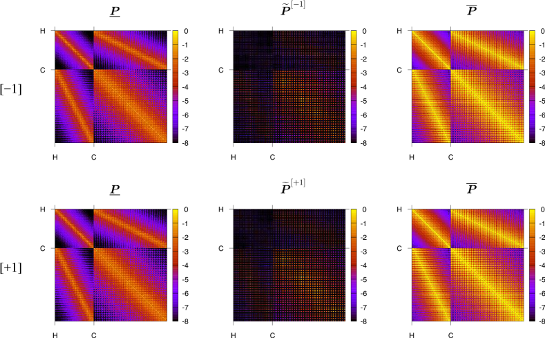
Figure 2: Maximum norm for each shell pair of core $\boldsymbol{\underline{P}}$, active $\boldsymbol{\widetilde{P}}$, and virtual pseudo-density matrices $\boldsymbol{\overline{P}}$ of the $\left[-1\right]$ and $\left[+1\right]$ contribution in the linear polyene chains $\text{C}_{32}\text{H}_{34}$. A CAS (8,8) space, SVP basis set,Schäfer, Horn, and Ahlrichs (1992) and a single quadrature point ($n_{\alpha}=1$) were used.

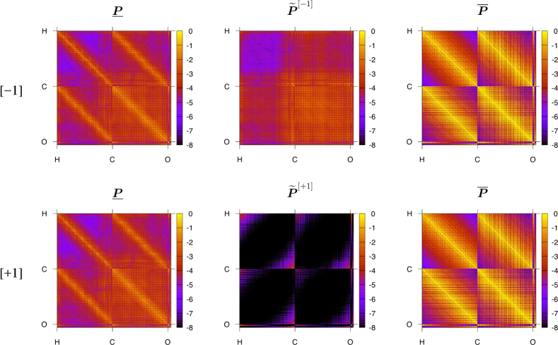
Figure 3: Maximum norm for each shell pair of core $\boldsymbol{\underline{P}}$, active $\boldsymbol{\widetilde{P}}$, and virtual pseudo-density matrices $\boldsymbol{\overline{P}}$ of the $\left[-1\right]$ and $\left[+1\right]$ contribution in the linear all-trans polyethylene glycol $\dot{\text{O}}-\text{C}_{32}\text{H}_{64}-\dot{\text{O}}$ biradical. A CAS (10,6) space, SVP basis set,Schäfer, Horn, and Ahlrichs (1992) and a single quadrature point ($n_{\alpha}=1$) were used.

Though the $\left[0\right]$, $\left[-1\right]$ and $\left[+1\right]$ energy terms show the same inter-electronic decay behavior, their magnitude may differ substantially and is sensitive to the number of electrons and orbitals in the active space. As $E^{\left[-1\right]}$ and $E^{\left[+1\right]}$ depend linearly on their respective active pseudo-density matrix, we show contour plots of $\boldsymbol{\widetilde{P}}^{\left[-1\right]}$ and $\boldsymbol{\widetilde{P}}^{\left[+1\right]}$ along with $\boldsymbol{\underline{P}}$ and $\boldsymbol{\overline{P}}$ for the polyene C${}_{\text{32}}$H${}_{\text{34}}$ (PE-32) and polyene glycol biradical $\dot{\text{O}}-\text{C}_{32}\text{H}_{64}-\dot{\text{O}}$ (PEG-32) in Figs. 2 and 3, respectively.si- The calculations were performed with the SVP basis setSchäfer, Horn, and Ahlrichs (1992) and the $1s$ orbitals of the C and O atoms were kept frozen. For PE-32 the CAS is composed of 8 electrons that are distributed amongst 8 active valence MOs. The latter are delocalized over the entire conjugated pi-system of the polyene. As can be see from Fig. 2, the active pseudo-density matrices $\boldsymbol{\widetilde{P}}^{\left[-1\right]}$ and $\boldsymbol{\widetilde{P}}^{\left[+1\right]}$ of the polyene are very similar and have their maxima along the diagonal of the C-C blocks. The elements of the H-H and H-C blocks of are much smaller in $\boldsymbol{\widetilde{P}}$. All $s$-type basis function do not contribute to the pi-orbitals in the CAS for symmetry reasons and, therefore, $\boldsymbol{\widetilde{P}}$ is much sparser than $\boldsymbol{\underline{P}}$ and $\boldsymbol{\overline{P}}$. For the PEG-32 biradical we build a CAS from the 10 electrons and 6 $2p$ orbitals of the two O atoms. Those active orbitals are localized at the ends of PEG-32 and have natural occupation numbers of $n_{\text{NO}}=(2.00,2.00,2.00,2.00,1.00,1.00)$. As can be seen from Fig. 3, the core and virtual pseudo-density matrices $\boldsymbol{\underline{P}}$ and $\boldsymbol{\overline{P}}$ have their largest elements at the diagonal shell pairs and their nearest neighbors whereas the largest elements of the active pseudo-densities $\boldsymbol{\widetilde{P}}$ are located at the O atoms. As expected from $n_{\text{NO}}$, $\boldsymbol{\widetilde{P}}^{\left[-1\right]}$ has much more significant elements than $\boldsymbol{\widetilde{P}}^{\left[+1\right]}$. Concerning $\boldsymbol{\widetilde{P}}^{\left[+1\right]}$, only those basis functions are important that have sizable coefficients for the two active MOs with $n_{\text{NO}}=1.00$.

The test molecules that we investigated have different physical characteristics of their valence orbitals in the active space. While for polyene the valence MOs are delocalized over nearly the whole molecule, for the polyethylene glycol biradical the valence MO are localized at the ends of the linear molecule. For both systems, we observed that the number of significant elements in the active pseudo-density matrix is much smaller than in the core and virtual pseudo-density matrix. In combination with the discussed $R^{-6}$ decay, this should pave the way for a reduced or even linearly scaling implementation where the ${\left[-1\right]}$ and ${\left[+1\right]}$ energies are formulated completely in the AO-basis. The computational overhead of an entirely AO-based formulation of the ${\left[-1\right]}$ and ${\left[+1\right]}$ energies can be reduced drastically when performing a CDZienau et al. (2009); Kussmann et al. (2015); Luenser, Schurkus, and Ochsenfeld of the active pseudo-density matrices. Such a CDD-based algorithm would combine successfully the sparsity with the low rank of active pseudo-density matrices.

IV.2 Accuracy of the numerical quadrature

The presence of three different orbital spaces results in eight different contributions to the IC first-order wavefunction contribution with eight different OEDs. Each of the 8 OEDs is approximated by its own numerical quadrature of its Laplace transform, which is determined by minimization the maximum absolute error (MAE) of the error distribution functionTakatsuka, Ten-no, and Hackbusch (2008)

$$\eta(\Delta) =\frac{1}{\Delta}-\sum_{\alpha=1}^{n_{\alpha}}\omega_{{\alpha}}\,\exp(-\Delta\,t_{{\alpha}})\text{.}$$ (53)

This procedure is known as the minimax algorithmTakatsuka, Ten-no, and Hackbusch (2008); Helmich-Paris and Visscher (2016) and can be performed in interval $[1,R]$ with $R=\Delta_{\text{max}}/\Delta_{\text{min}}$ by scaling the parameters $\{\omega_{\alpha},t_{\alpha}\}$. This facilitates pre-tabulation of $\{\omega_{\alpha},t_{\alpha}\}$ along with their MAEs $\delta_{n_{\alpha},[1,R^{\prime}]}$ for some discrete $R^{\prime}$. These $2n_{\alpha}+1$ parameters can be used as start values in the iterative optimization procedure.Hackbusch (2007) We choose $n_{\alpha}$ such that

$$\delta_{n_{\alpha},[1,R^{\prime}]}\leq T_{\text{lap}}\text{ with }R\leq R^{\prime}$$ (54)

where $R^{\prime}$ is the pre-tabulated range closest to $R$. The accuracy of the numerical quadrature depends on a single user-given threshold $T_{\text{lap}}$ that should correlate with the resultant error in each correlation energy contribution. Alternatively, one could simply set $n_{\alpha}$ to the same value for each of the 8 OEDs based on experience. However, by doing so, the errors in $E^{(2)}$ cannot be easily controlled for each class. This can be clearly seen from Fig. 1 where the 8 different $E^{(2)}$ errors differ from each other even by more than 4 orders of magnitude for some $n_{\alpha}$. Conversely, the same $E^{(2)}$ errors converge much more uniformly with respect to the MAE $\delta_{n_{\alpha},[1,R]}$, as shown in Fig. 1.

In the following, we investigate the $E^{(2)}$ errors when $n_{\alpha}$ is selected according to (54) for the ground state ${{}^{1}}\Sigma_{g}^{+}$ of the fluorine and chlorine dimer. The results for different computational setups are compiled in Tab. 4. For F${}_{\text{2}}$ and Cl${}_{\text{2}}$ (a multiple of) the equilibrium bond distances $(n\times)r_{eq}$ were taken from experimental data.Huber and Herzberg (2015) For F the cc-pVTZDunning (1989) and aug-cc-pVTZKendall, Dunning, and Harrison (1992) basis sets were employed; for Cl we used the cc-pwCVTZWoon and Jr. (1993) basis set. The Laplace accuracy threshold $T_{\text{lap}}$ was set to $10^{-7}$. We note that for all calculations in Tab. 4 the $\left[+1\right]^{\prime}$ part of the $E^{(2)}$ is zero and is not shown.

For the first two $E^{(2)}$ calculation of F${}_{\text{2}}$ in Tab. 4 we chose a CAS (10,6) that includes all $2p$ orbitals and electrons of F. The first calculation differs from the second only in correlation of the 1s core orbitals. The 8 OED ranges $R$ of the all-electron (AE) calculation varies roughly by a factor of two only and similar $n_{\alpha}$, i. e. 7 and 8, are selected by our procedure. The absolute errors in $E^{(2)}$ are all below $10^{-9}$. By freezing the $1s$ orbitals the OED ranges of those classes that involve core orbitals are decreased significantly while the $\left[-2\right]$ and $\left[-1\right]^{\prime}$ contributions remain unchanged. The latter require the least $n_{\alpha}$ (7) in the AE calculation but the most in the frozen-core (FC) calculation. For the FC calculation the OED ranges differ by almost 1 order of magnitude. Nevertheless, all absolute errors in $E^{(2)}$ are smaller than $10^{-8}$. Augmenting the cc-pVTZ basis by one diffuse basis function for each angular momentumKendall, Dunning, and Harrison (1992) lowers the eigenvalues of the virtual-virtual block of the Fock matrix. We can observe for the third calculation in Tab. 4 that the OED ranges of those classes that involve virtual orbitals are increased approximately by a factor of 2 while those of the $\left[+2\right]$ space are almost unaffected when adding the diffuse “aug-” functions to the basis set. The absolute errors in $E^{(2)}$ are still reliably below $10^{-9}$.

For Cl atom in Cl${}_{\text{2}}$ we correlate the $2s2p3s3p$ orbitals and keep the $1s$ frozen. For the fourth calculation in Tab. 4 we put the all $3p$ orbitals and electrons of Cl into the active space, that is CAS (10,6). For this calculation the OED ranges become much larger than those of the FC F${}_{\text{2}}$ calculations, which can be attributed to the additional core electrons and the larger basis set for Cl. The largest OED range in the fourth calculation is 114.76, while the largest in F${}_{\text{2}}$ calculation with the aug-cc-pVTZ basis set is 24.32. Though the OED ranges vary by more than 1 order of magnitude for the Cl${}_{\text{2}}$ calculation, all absolute errors in $E^{(2)}$ are less than $10^{-8}$ and $n_{\alpha}$ seems to be selected properly. In the fifth calculation in Tab. 4 the $3s$ orbitals and electrons of the Cl atoms are included in the valence space, i. e. CAS (14,8). This lowers substantially the OED ranges of all those classes that excite from core electrons. The smallest ($\left[+2\right]$) and the largest OED range ($\left[-1\right]^{\prime}$) differ by almost 2 orders of magnitude but $n_{\alpha}$ is selected properly as the absolute error in $E^{(2)}$ is always smaller $10^{-8}$. The convergence of the absolute $E^{(2)}$ error with respect to $n_{\alpha}$ and the MAE $\delta_{n_{\alpha},[1,R]}$ is shown in Fig. 1 and has been discussed already in the beginning of this section.

The previous example calculations of F${}_{\text{2}}$ and Cl${}_{\text{2}}$ had clearly single-reference character as deduced from their natural occupation numbers ($n_{\text{NO}}>1.85$ or $n_{\text{NO}}<0.15$) and could have been performed more easily with closed-shell single-reference MP2 or coupled cluster. Therefore, we performed the CAS (14,8) calculation also on a stretched Cl${}_{\text{2}}$ with $3\times r_{eq}$ bond distance. Now there are 2 open shells with $n_{\text{NO}}=1.00$ and 6 closed shells with $n_{\text{NO}}=2.00$. As we investigate the ${{}^{1}}\Sigma^{+}_{g}$ state of Cl${}_{\text{2}}$, at least 2 CSF are required to describe the system at least qualitatively correct. Thus, he have a MR case by definition. The MR character does not seem to change the OEDs much and we obtain absolute errors in $E^{(2)}$ that are all smaller than $10^{-8}$. It is noteworthy that the $\left[+2\right]$ contribution to the correlation energy almost vanishes since Cl${}_{\text{2}}$ can be considered as nearly dissociated at $3\times r_{eq}$ and it is impossible to attach 2 electrons into a CAS (5,3) or (7,4) valence space of a single Cl atom.

A further field of application of MRPT methods are excited states. With our state-specific (SS) Laplace-transformed PC-NEVPT2 method we investigate the OED ranges and absolute errors in $E^{(2)}$ of the ground state 1 ${}^{\text{1}}$A${}_{\text{1}}$ and two lowest vertically excited singlet states 1 ${}^{\text{1}}$A${}_{\text{2}}$ ($n_{y}\to\pi^{*}$) and 1 ${}^{\text{1}}$B${}_{\text{2}}$ ($n_{y}\to 3s$) in formaldehyde, which are shown in Tab. 5. Those and other valence and Rydberg excited states have been investigated rigorously by Merchán and RoosMerchán and Roos (1995) with SS-CASPT2 and by Angeli et al. with SS-NEVPT2Angeli, Borini, and Cimiraglia (2004). The geometry and the ANO(S)-Ryd(S) basis set were taken from their works. To describe also Rydberg states, a contracted s, p, and d function, denoted by Ryd(S), were located altogether in the geometric center of H${}_{\text{2}}$CO. In contrast to Refs. Merchán and Roos, 1995 and Angeli, Borini, and Cimiraglia, 2004 we chose a CAS (4,4) that includes the $(1b_{1},2b_{2},6a_{1},2b_{1})$ orbitals to optimize the orbitals and CI coefficients of the 1 ${}^{\text{1}}$A${}_{\text{1}}$, 1 ${}^{\text{1}}$A${}_{\text{2}}$, and 1 ${}^{\text{1}}$B${}_{\text{2}}$ states simultaneously in the SA-CASSCF procedure because, currently, we cannot exploit PG symmetry for the NEVPT2 calculations with our pilot implementation. Nevertheless, the excitation energies to the 1 ${}^{\text{1}}$A${}_{\text{2}}$ (4.10 eV) and 1 ${}^{\text{1}}$B${}_{\text{2}}$ state (7.18 eV) differ only by -0.07 and +0.10 eV, respectively, though an active space was employed that differs from the ones of Ref. Angeli, Borini, and Cimiraglia, 2004.

As observed already for the halogen dimers, those classes that attach electrons into the active space have the smallest OED ranges and demand the least $n_{\alpha}$ to reach a desired accuracy for all 3 states in Tab. 5; while active space electron ionization classes have larger OED ranges and need the most $n_{\alpha}$. The combined single electron ionization and excitation class $\left[-1\right]^{\prime}$ has the largest OED range for each of the 3 states but does not contribute with more than 7 % to the total $E^{(2)}$ energy. For the Rydberg excited state 1 ${}^{\text{1}}$B${}_{\text{2}}$ the OED range of the $\left[-1\right]^{\prime}$ class is only a factor of two larger than for both the ground state 1 ${}^{\text{1}}$A${}_{\text{1}}$ and first valence excited state 1 ${}^{\text{1}}$A${}_{\text{2}}$. Furthermore, only 1 additional quadrature point is required for $\left[-1\right]^{\prime}$ in 1 ${}^{\text{1}}$B${}_{\text{2}}$ to reach the requested target accuracy. Therefore, OED ranges of $E^{(2)}$ contributions to Rydberg excited states are larger than for valence excited states; but even if diffuse basis functions are included in the basis set, the additional number of quadrature points is still rather decent. In fact, it is the less effective screening of shell contributions in the AO basis rather than the additional number of quadrature points that makes an AO-based formulation less powerful for basis sets with diffuse basis functions in a production-level implementation. This we will study in future work.

V Conclusions

In the present article we showed how to formulate the partially contracted n-electron valence second order perturbation theory (PC-NEVPT2) energies in the atomic and active molecular orbital basis by employing the Laplace transformation of orbital-energy denominators (OED). As the number of active orbitals is comparatively small and AO basis functions are inherently localized, our formulation is particularly suited for a linearly-scaling NEVPT2 implementation. Some of the NEVPT2 energy contributions can be formulated completely in the AO basis as single-reference second-order Møller–Plesset perturbation theory and benefit from sparse active-pseudo density matrices — particularly if the active molecular orbitals are localized only in parts of a molecule. Furthermore, we could show that finding optimal parameters of the numerical Laplace transformation is particularly challenging for multi-reference perturbation theories as the fit range may vary among the 8 different OEDs by many orders of magnitude. Selecting the number of quadrature points for each OED separately according to an accuracy-based criterion allows us to control the errors in the NEVPT2 energies reliably. Currently, we work on efficient low-order scaling implementations of NEVPT2 and relativistic two-component MP2. The extension of our formalism to quasi-degenerate NEVPT2Angeli et al. (2004) or the uncontracted time-dependent NEVPT2Sokolov and Chan (2016) will be presented in the future.

VI Acknowledgments

This work was supported by the the German research foundation DFG through a research fellowship (Grant No. HE 7427/1-1) and the Dutch science foundation NWO through a VENI fellowship (Grant No. 722.016.011). B. H.-P. would like to thank Markus Reiher for granting access to the local computing facilities at ETH Zürich and the NWO for computer time at the Dutch national supercomputers. The authors also thank Hans Jørgen Aa. Jensen for sharing his experiences in multi-reference electronic structure methods.

Figure 1: Numerical integration errors in Laplace-transformed AO-NEVPT2 energies for Cl₂ (r${}_{\text{eq}}$ = 1.9879 Å, CAS (14,8), cc-pwCVTZ basis set, 1s orbitals frozen) with respect to the number of quadrature points 1 and the maximum absolute error of Eq. (53) in 1.

Table 1: Explicit expressions for the Laplace-transformed PC-NEVPT2 energies and their intermediates in the atomic and active molecular orbital basis.

$$E^{\left[0\right]}=-\sum_{\alpha}\,\sum_{\mu\nu\kappa\lambda}(\underline{\mu}\bar{\nu}|\kappa\lambda)^{(\alpha)}\Big{[}2(\mu\nu|\underline{\kappa}\bar{\lambda})^{(\alpha)}-(\mu\bar{\lambda}|\underline{\kappa}\nu)^{(\alpha)}\Big{]}$$

$$E^{\left[-1\right]}=-\sum_{\alpha}\sum_{\mu\nu\kappa\lambda}(\underline{\mu}\bar{\nu}|\kappa\lambda)^{(\alpha)}\Big{[}2(\mu\nu|\tilde{\kappa}^{\left[-1\right]}\bar{\lambda})^{(\alpha)}-(\mu\bar{\lambda}|\tilde{\kappa}^{\left[-1\right]}\nu)^{(\alpha)}\Big{]}$$

$$E^{\left[+1\right]}=-\sum_{\alpha}\sum_{\mu\nu\kappa\lambda}(\underline{\mu}\bar{\nu}|\kappa\lambda)^{(\alpha)}\Big{[}2(\mu\nu|\underline{\kappa}\tilde{\lambda}^{[+1]})^{(\alpha)}-(\mu\tilde{\lambda}^{[+1]}|\underline{\kappa}\nu)^{(\alpha)}\Big{]}$$

$$E^{\left[-2\right]}=-\frac{1}{2}\sum_{\alpha}\sum_{\begin{subarray}{c}\nu\lambda\\ tut^{\prime}u^{\prime}\end{subarray}}(t\nu|u\lambda)\,\mathcal{K}^{(\alpha),\left[-2\right]}_{tu,t^{\prime}u^{\prime}}\,(t^{\prime}\bar{\nu}|u^{\prime}\bar{\lambda})^{(\alpha)}$$

$$E^{\left[+2\right]}=-\frac{1}{2}\sum_{\alpha}\sum_{\begin{subarray}{c}\mu\kappa\\ tut^{\prime}u^{\prime}\end{subarray}}(\mu t|\kappa u)\,\mathcal{K}^{(\alpha),\left[+2\right]}_{tu,t^{\prime}u^{\prime}}\,(\underline{\mu}t^{\prime}|\underline{\kappa}u^{\prime})^{(\alpha)}$$

$$E^{\left[-1\right]^{\prime}}=-\sum_{\alpha}\sum_{\begin{subarray}{c}\mu\\ tuvt^{\prime}u^{\prime}v^{\prime}\end{subarray}}\widetilde{(\mu u|tv)}^{\left[-1\right]^{\prime}}\,\mathcal{K}^{(\alpha),\left[-1\right]^{\prime}}_{tuv,t^{\prime}u^{\prime}v^{\prime}}\widetilde{({\bar{\mu}}u^{\prime}|t^{\prime}v^{\prime})}^{(\alpha),\left[-1\right]^{\prime}}$$

$$E^{\left[+1\right]^{\prime}}=-\sum_{\alpha}\sum_{\begin{subarray}{c}\mu\\ tuvt^{\prime}u^{\prime}v^{\prime}\end{subarray}}\widetilde{(\mu u|tv)}^{\left[+1\right]^{\prime}}\,\mathcal{K}^{(\alpha),\left[+1\right]^{\prime}}_{tuv,t^{\prime}u^{\prime}v^{\prime}}\,\widetilde{(\underline{\mu}u^{\prime}|t^{\prime}v^{\prime})}^{(\alpha),\left[+1\right]^{\prime}}$$

$$E^{\left[0\right]^{\prime}}=-\sum_{\alpha}\sum_{\begin{subarray}{c}\mu\nu\\ tut^{\prime}u^{\prime}\end{subarray}}\Big{[}\widetilde{(\mu\nu|tu)}^{\left[0\right]^{\prime}}\,\mathcal{K}^{(\alpha),\left[0\right]^{\prime},AA}_{tu,t^{\prime}u^{\prime}}\,\widetilde{(\underline{\mu}\bar{\nu}|t^{\prime}u^{\prime})}^{(\alpha),\left[0\right]^{\prime}}$$

$$\phantom{E^{\left[0\right]^{\prime}}=-\sum_{\alpha}\sum_{\begin{subarray}{c}\mu\nu\\ tut^{\prime}u^{\prime}\end{subarray}}}+2\widetilde{(\mu\nu|tu)}^{\left[0\right]^{\prime}}\,\mathcal{K}^{(\alpha),\left[0\right]^{\prime},AB}_{tu,t^{\prime}u^{\prime}}\,(\underline{\mu}u^{\prime}|t^{\prime}\bar{\nu})^{(\alpha)}$$

$$\phantom{E^{\left[0\right]^{\prime}}=-\sum_{\alpha}\sum_{\begin{subarray}{c}\mu\nu\\ tut^{\prime}u^{\prime}\end{subarray}}}+(\mu u|t\nu)\,\mathcal{K}^{(\alpha),\left[0\right]^{\prime},BB}_{tu,t^{\prime}u^{\prime}}\,(\underline{\mu}u^{\prime}|t^{\prime}\bar{\nu})^{(\alpha)}\Big{]}$$

$$(\mu\nu|\underline{\kappa}\tilde{\lambda}^{[+1]})^{(\alpha)}=\sum_{\kappa^{\prime}}\underline{P}_{\kappa\kappa^{\prime}}^{(\alpha)}\sum_{\lambda^{\prime}}\widetilde{P}_{\lambda\lambda^{\prime}}^{(\alpha),\left[+1\right]}\,(\mu\nu|\kappa^{\prime}\lambda^{\prime})$$

$$\widetilde{(\mu\nu|tu)}^{\left[0\right]^{\prime}}=(\mu\nu|tu)+f_{\mu\nu}^{\text{I}}\sum_{vw}\gamma_{vw}[(\mathbf{M}^{\left[0\right]^{\prime}})^{-1}]_{tu,vw}$$

$$\widetilde{(\mu t|uv)}^{\left[-1\right]^{\prime}}=(\mu t|uv)+\sum_{w}f^{\prime I}_{\mu w}\sum_{tuv}(\Gamma_{vu,tw}+\delta_{tu}\,\gamma_{vw})\,\sum_{\tau}c_{tuv,\tau}^{\left[-1\right]^{\prime}}\,c_{tuv,\tau}^{\left[-1\right]^{\prime}}$$

$$\widetilde{(\mu t|uv)}^{\left[+1\right]^{\prime}}=(\mu t|uv)+\sum_{w}f^{I}_{\mu w}\sum_{tuv}(2\delta_{uw}\gamma_{vt}-\delta_{tw}\gamma_{vu}-\Gamma_{vw,tu})\,\sum_{\tau}c_{tuv,\tau}^{\left[+1\right]^{\prime}}\,c_{tuv,\tau}^{\left[+1\right]^{\prime}}$$

$$f^{\prime\text{I}}_{\mu t}=f^{\text{I}}_{\mu t}-(\mu u|ut)$$

$$\widetilde{P}_{\mu\mu^{\prime}}^{(\alpha),\left[+1\right]}=\sum_{t}C_{\mu t}\,\sum_{t^{\prime}}\mathcal{K}^{(\alpha),\left[+1\right]}_{tt^{\prime}}\,C_{\mu^{\prime}u^{\prime}}$$

Table 2: Metric matrices for each class (top) formulated in terms of singlet reduced density matrices (bottom)

$$M^{\left[-1\right]}_{tt^{\prime}}=\gamma_{tt^{\prime}}$$

$$M^{\left[+1\right]}_{tt^{\prime}}=2\delta_{tt^{\prime}}-\gamma_{t^{\prime}t}$$

$$M^{\left[-2\right]}_{tu,t^{\prime}u^{\prime}}=\Gamma_{tu,t^{\prime}u^{\prime}}$$

$$M^{\left[+2\right]}_{tu,t^{\prime}u^{\prime}}=\Gamma_{tu,t^{\prime}u^{\prime}}+4\,\delta_{tt^{\prime}}\,\delta_{uu^{\prime}}-2\,\delta_{tu^{\prime}}\,\delta_{ut^{\prime}}$$

$$\phantom{M^{\left[+2\right]}_{tu,t^{\prime}u^{\prime}}=}-2\,\delta_{tt^{\prime}}\,\gamma_{uu^{\prime}}+\delta_{tu^{\prime}}\,\gamma_{ut^{\prime}}-2\,\delta_{uu^{\prime}}\,\gamma_{tt^{\prime}}+\delta_{ut^{\prime}}\,\gamma_{tu^{\prime}}$$

$$M^{\left[-1\right]^{\prime}}_{tuv,t^{\prime}u^{\prime}v^{\prime}}=\delta_{tu}\,\delta_{t^{\prime}u^{\prime}}\,\gamma_{vv^{\prime}}+\delta_{t^{\prime}u^{\prime}}\,\Gamma_{vu,tv^{\prime}}+\delta_{tu}\,\Gamma_{vt^{\prime},u^{\prime}v^{\prime}}$$

$$\phantom{M^{\left[-1\right]^{\prime}}_{tuv,t^{\prime}u^{\prime}v^{\prime}}=}+\delta_{tt^{\prime}}\,\Gamma_{vu,v^{\prime}u^{\prime}}+\Gamma_{vut^{\prime},tu^{\prime}v^{\prime}}$$

$$M^{\left[+1\right]^{\prime}}_{tuv,t^{\prime}u^{\prime}v^{\prime}}=2\,\delta_{tt^{\prime}}\,\delta_{uu^{\prime}}\,\gamma_{vv^{\prime}}+2\,\delta_{uu^{\prime}}\,\Gamma_{vt^{\prime},tv^{\prime}}-M^{\left[-1\right]^{\prime}}_{tu^{\prime}v,t^{\prime}uv^{\prime}}$$

$$\mathbf{M}^{\left[0\right]^{\prime}}=\left[\begin{array}[]{cc}2\mathbf{M}^{AA}&-\mathbf{M}^{AB}\\ -\mathbf{M}^{BA}&\mathbf{M}^{BB}\end{array}\right]$$

$$\mathbf{M}^{AA}=\mathbf{M}^{AB}=\mathbf{M}^{BA}=M^{\left[0\right]^{\prime}}_{tu,t^{\prime}u^{\prime}}=\delta_{uu^{\prime}}\,\gamma_{tt^{\prime}}+\Gamma_{tu^{\prime},ut^{\prime}}$$

$$\mathbf{M}^{BB}=M^{\prime\left[0\right]^{\prime}}_{tu,t^{\prime}u^{\prime}}=2\,\delta_{uu^{\prime}}\,\gamma_{tt^{\prime}}-\Gamma_{u^{\prime}t,ut^{\prime}}$$

$$\gamma_{tt^{\prime}}=\sum_{\sigma}\langle 0|a^{{\dagger}}_{t\sigma}a_{t^{\prime}\sigma}|0\rangle$$

$$\Gamma_{tu,t^{\prime}u^{\prime}}=\sum_{\sigma\sigma^{\prime}}\langle 0|a^{{\dagger}}_{t\sigma}a^{{\dagger}}_{u\sigma^{\prime}}a_{u^{\prime}\sigma^{\prime}}a_{t^{\prime}\sigma}|0\rangle$$

$$\Gamma_{tuv,t^{\prime}u^{\prime}v^{\prime}}=\sum_{\sigma\sigma^{\prime}\sigma^{\prime\prime}}\langle 0|a^{{\dagger}}_{t\sigma}a^{{\dagger}}_{u\sigma^{\prime}}a^{{\dagger}}_{v\sigma^{\prime\prime}}a_{v^{\prime}\sigma^{\prime\prime}}a_{u^{\prime}\sigma^{\prime}}a_{t^{\prime}\sigma}|0\rangle$$

$$\Gamma_{tuvw,t^{\prime}u^{\prime}v^{\prime}w^{\prime}}=\sum_{\sigma\sigma^{\prime}\sigma^{\prime\prime}\sigma^{\prime\prime\prime}}\langle 0|a^{{\dagger}}_{t\sigma}a^{{\dagger}}_{u\sigma^{\prime}}a^{{\dagger}}_{v\sigma^{\prime\prime}}a^{{\dagger}}_{w\sigma^{\prime\prime\prime}}a_{w^{\prime}\sigma^{\prime\prime\prime}}a_{v^{\prime}\sigma^{\prime\prime}}a_{u^{\prime}\sigma^{\prime}}a_{t^{\prime}\sigma}|0\rangle$$

Table 3: Definition of the internally contracted configurations (ICC) for the 8 excitation classes. For CASPT2 and PC-NEVPT2 the projection manifold is built from a bi-orthogonal ICC basis while for SC-NEVPT2 a special basis is chosen with contraction over all active orbitals.

label	$|\text{ICC}\rangle$	$\langle\text{ICC}|$	SC $\langle\text{ICC}|$
$\left[0\right]$	$|\Phi_{ij}^{ab}\rangle=\hat{E}_{ai}\hat{E}_{bj}|0\rangle$	$\langle\widetilde{\Phi_{ij}^{ab}}|=\frac{1}{6}\langle 0|\Big{(}2\,\hat{E}_{jb}\hat{E}_{ia}+\hat{E}_{ib}\hat{E}_{ja}\Big{)}$
$\left[-1\right]$	$|\Phi_{it}^{ab}\rangle=\hat{E}_{ai}\hat{E}_{bt}|0\rangle$	$\langle\widetilde{\Phi_{it}^{ab}}|=\frac{1}{3}\langle 0|\Big{(}2\,\hat{E}_{tb}\hat{E}_{ia}+\hat{E}_{ib}\hat{E}_{ta}\Big{)}$	$\langle\widetilde{\Phi_{i}^{ab}}|=\frac{1}{3}\sum_{t}g_{tbia}\langle 0|\Big{(}2\,\hat{E}_{tb}\hat{E}_{ia}+\hat{E}_{ib}\hat{E}_{ta}\Big{)}$
$\left[+1\right]$	$|\Phi_{ij}^{at}\rangle=\hat{E}_{ai}\hat{E}_{tj}|0\rangle$	$\langle\widetilde{\Phi_{ij}^{at}}|=\frac{1}{3}\langle 0|\Big{(}2\,\hat{E}_{jt}\hat{E}_{ia}+\hat{E}_{it}\hat{E}_{ja}\Big{)}$	$\langle\widetilde{\Phi_{ij}^{a}}|=\frac{1}{3}\sum_{t}g_{jtia}\langle 0|\Big{(}2\,\hat{E}_{jt}\hat{E}_{ia}+\hat{E}_{it}\hat{E}_{ja}\Big{)}$
$\left[-2\right]$	$|\Phi_{tu}^{ab}\rangle=\hat{E}_{at}\hat{E}_{bu}|0\rangle$	$\langle\widetilde{\Phi_{tu}^{ab}}|=\langle 0|\hat{E}_{ub}\hat{E}_{ta}$	$\langle\widetilde{\Phi^{ab}}|=\sum_{tu}g_{ubta}\langle 0|\hat{E}_{ub}\hat{E}_{ta}$
$\left[+2\right]$	$|\Phi_{ij}^{tu}\rangle=\hat{E}_{ti}\hat{E}_{uj}|0\rangle$	$\langle\widetilde{\Phi_{ij}^{tu}}|=\langle 0|\hat{E}_{ju}\hat{E}_{ti}$	$\langle\widetilde{\Phi_{ij}}|=\sum_{tu}g_{juti}\langle 0|\hat{E}_{ju}\hat{E}_{ti}$
$\left[-1\right]^{\prime}$	$|\Phi_{tu}^{av}\rangle=\hat{E}_{at}\hat{E}_{vu}|0\rangle$	$\langle\widetilde{\Phi_{tu}^{av}}|=\langle 0|\hat{E}_{uv}\hat{E}_{ta}$	$\langle\widetilde{\Phi^{a}}|=\sum_{tuv}g_{uvta}\langle 0|\hat{E}_{uv}\hat{E}_{ta}+\sum_{t}f^{\prime\text{I}}_{ta}\langle 0|\hat{E}_{ta}$
$\left[+1\right]^{\prime}$	$|\Phi_{it}^{uv}\rangle=\hat{E}_{ui}\hat{E}_{vt}|0\rangle$	$\langle\widetilde{\Phi_{it}^{uv}}|=\langle 0|\hat{E}_{tv}\hat{E}_{iu}$	$\langle\widetilde{\Phi_{i}}|=\sum_{tuv}g_{tviu}\langle 0|\hat{E}_{tv}\hat{E}_{iu}+\sum_{t}f^{\text{I}}_{it}\langle 0|\hat{E}_{it}$
$\left[0\right]^{\prime}$	$|\Phi_{it}^{au}\rangle=\hat{E}_{ai}\hat{E}_{ut}|0\rangle$,	$\langle\widetilde{\Phi_{it}^{au}}|=\langle 0|\hat{E}_{tu}\hat{E}_{ia}$,	$\langle\widetilde{\Phi_{i}^{a}}|=\sum_{tu}\Big{(}g_{tuia}\langle 0|\hat{E}_{tu}\hat{E}_{ia}+g_{taiu}\hat{E}_{ta}\hat{E}_{iu}\Big{)}$
	$|\Phi_{it}^{ua}\rangle=\hat{E}_{ui}\hat{E}_{at}|0\rangle$	$\langle\widetilde{\Phi_{it}^{ua}}|=\langle 0|\hat{E}_{ta}\hat{E}_{iu}$	$\phantom{\langle\widetilde{\Phi_{i}^{a}}|=}+f^{\text{I}}_{ia}\langle 0|\hat{E}_{ia}$

Table 4: Errors ($\Delta E$) of the numerical quadrature and reference ($E_{\text{ref}}$) for each PC-NEVPT2 energy contribution of Cl${}_{\text{2}}$ and F${}_{\text{2}}$ in the ground state ${{}^{1}}\Sigma_{g}^{+}$. The target accuracy for the determination of the number of quadrature points $n_{\alpha}$ was set to $T_{\text{lap}}=10^{-7}$.

class	$E_{\text{ref}}$ / a. u.	$\Delta E$ / a. u.	$R$	$n_{\alpha}$
F${}_{\text{2}}$ (r${}_{\text{eq}}$), cc-pVTZ, CAS (10,6), AE
$\left[0\right]$	-0.030025488553	$3.17\times 10^{-10}$	16.37	8
$\left[-1\right]$	-0.111943993847	$7.13\times 10^{-10}$	13.29	8
$\left[+1\right]$	-0.002340179047	$3.00\times 10^{-11}$	16.13	8
$\left[-2\right]$	-0.212848549931	$-8.08\times 10^{-10}$	7.47	7
$\left[+2\right]$	-0.001439019119	$1.00\times 10^{-11}$	12.99	8
$\left[0\right]^{\prime}$	-0.047509476974	$-6.97\times 10^{-10}$	16.90	8
$\left[-1\right]^{\prime}$	-0.043202501004	$6.10\times 10^{-10}$	9.44	7
sum	-0.449309208510	$1.75\times 10^{-10}$
F${}_{\text{2}}$ (r${}_{\text{eq}}$), cc-pVTZ, CAS (10,6), 1s frozen
$\left[0\right]$	-0.018579052395	$-1.00\times 10^{-11}$	5.53	6
$\left[-1\right]$	-0.100501783485	$-3.87\times 10^{-09}$	6.65	6
$\left[+1\right]$	-0.001394951164	$4.80\times 10^{-11}$	3.78	5
$\left[-2\right]$	-0.212848549931	$-8.08\times 10^{-10}$	7.47	7
$\left[+2\right]$	-0.001368251581	$<10^{-12}$	1.12	3
$\left[0\right]^{\prime}$	-0.046541048840	$-2.84\times 10^{-10}$	6.05	6
$\left[-1\right]^{\prime}$	-0.043202501004	$6.10\times 10^{-10}$	9.44	7
sum	-0.424436138435	$-4.31\times 10^{-09}$
F${}_{\text{2}}$ (r${}_{\text{eq}}$), aug-cc-pVTZ, CAS (10,6), 1s frozen
$\left[0\right]$	-0.018942769474	$4.80\times 10^{-11}$	10.65	8
$\left[-1\right]$	-0.104717284874	$9.60\times 10^{-10}$	14.15	8
$\left[+1\right]$	-0.001432889156	$2.00\times 10^{-12}$	5.93	6
$\left[-2\right]$	-0.218661812847	$5.58\times 10^{-09}$	16.88	8
$\left[+2\right]$	-0.001372612217	$<10^{-12}$	1.12	3
$\left[0\right]^{\prime}$	-0.046967568913	$5.60\times 10^{-11}$	11.39	8
$\left[-1\right]^{\prime}$	-0.044436625063	$3.16\times 10^{-10}$	24.32	9
sum	-0.436531562544	$6.96\times 10^{-09}$
Cl${}_{\text{2}}$ (r${}_{\text{eq}}$), cc-pwCVTZ, CAS (10,6), 1s frozen
$\left[0\right]$	-0.471288060730	$5.03\times 10^{-09}$	72.20	10
$\left[-1\right]$	-0.156827410078	$-5.59\times 10^{-09}$	86.56	10
$\left[+1\right]$	-0.015084015071	$1.26\times 10^{-09}$	43.77	9
$\left[-2\right]$	-0.178487055950	$-8.42\times 10^{-09}$	93.65	10
$\left[+2\right]$	-0.001461454900	$7.00\times 10^{-12}$	7.93	7
$\left[0\right]^{\prime}$	-0.042764807405	$4.76\times 10^{-10}$	72.86	10
$\left[-1\right]^{\prime}$	-0.028430997436	$-2.44\times 10^{-10}$	114.76	11
sum	-0.894343801571	$-7.47\times 10^{-09}$
Cl${}_{\text{2}}$ (r${}_{\text{eq}}$), cc-pwCVTZ, CAS (14,8), 1s frozen
$\left[0\right]$	-0.423057258482	$4.96\times 10^{-10}$	11.86	8
$\left[-1\right]$	-0.108905246973	$1.01\times 10^{-10}$	20.62	9
$\left[+1\right]$	-0.009006319960	$2.42\times 10^{-10}$	6.71	6
$\left[-2\right]$	-0.261212365274	$-4.11\times 10^{-09}$	94.37	10
$\left[+2\right]$	-0.000139138179	$1.00\times 10^{-12}$	1.30	3
$\left[0\right]^{\prime}$	-0.007634923746	$5.00\times 10^{-12}$	12.10	8
$\left[-1\right]^{\prime}$	-0.067654717180	$-1.35\times 10^{-10}$	117.33	11
sum	-0.877609969794	$-3.40\times 10^{-09}$
Cl${}_{\text{2}}$ (3$\times$r${}_{\text{eq}}$), cc-pwCVTZ, CAS (14,8), 1s frozen
$\left[0\right]$	-0.424002208658	$4.54\times 10^{-10}$	11.64	8
$\left[-1\right]$	-0.113366194595	$-7.23\times 10^{-10}$	19.93	8
$\left[+1\right]$	-0.005732731250	$1.91\times 10^{-10}$	6.66	6
$\left[-2\right]$	-0.250053179564	$-7.97\times 10^{-09}$	90.82	10
$\left[+2\right]$	-0.000000000704	$<10^{-12}$	1.31	3
$\left[0\right]^{\prime}$	-0.005920160948	$-7.00\times 10^{-12}$	11.83	8
$\left[-1\right]^{\prime}$	-0.049804208204	$-3.75\times 10^{-09}$	97.24	10
sum	-0.848878684178	$-1.18\times 10^{-08}$

Table 5: Errors ($\Delta E$) of the numerical quadrature and reference ($E_{\text{ref}}$) for each PC-NEVPT2 energy contribution to the three lowest singlet states of formaldehyde. The natural occupation numbers in the CAS (4,4) are provide as $(1b_{1},2b_{2},6a_{1},2b_{1})$. The target accuracy for the determination of the number of quadrature points $n_{\alpha}$ was set to $T_{\text{lap}}=10^{-7}$. The ANO(S)-Ryd(S) basis set of Ref. Angeli, Borini, and Cimiraglia, 2004 was employed. The $1s$ orbitals of the C and O atom were kept frozen in the PT calculation.

class	$E_{\text{ref}}$ / a. u.	$\Delta E$ / a. u.	$R$	$n_{\alpha}$
1${}^{\text{1}}$A${}_{\text{1}}$, (1.90,2.00,0.00,0.10)
$\left[0\right]$	-0.100574701804	$-9.00\times 10^{-12}$	10.33	8
$\left[-1\right]$	-0.101361528657	$-7.00\times 10^{-12}$	11.86	8
$\left[+1\right]$	-0.012154365169	$3.10\times 10^{-11}$	6.51	6
$\left[-2\right]$	-0.035050155679	$-4.55\times 10^{-10}$	9.80	7
$\left[+2\right]$	-0.001562160519	$2.00\times 10^{-12}$	2.39	5
$\left[0\right]^{\prime}$	-0.045498719711	$-7.10\times 10^{-11}$	12.00	8
$\left[-1\right]^{\prime}$	-0.021615019596	$3.90\times 10^{-11}$	20.34	9
$\left[+1\right]^{\prime}$	-0.000839589656	$4.00\times 10^{-12}$	4.24	6
sum	-0.318656240791	$-4.66\times 10^{-10}$
1 ${}^{\text{1}}$A${}_{\text{2}}$ (n${}_{\text{y}}$ $\to$ $\pi^{*}$), (2.00,1.00,0.00,1.00)
$\left[0\right]$	-0.100706612983	$-5.00\times 10^{-12}$	10.48	8
$\left[-1\right]$	-0.101295292993	$-8.40\times 10^{-11}$	14.04	8
$\left[+1\right]$	-0.019711077239	$-8.20\times 10^{-11}$	6.44	6
$\left[-2\right]$	-0.030702543569	$3.00\times 10^{-12}$	10.37	8
$\left[+2\right]$	-0.000285995858	$<10^{-12}$	2.40	5
$\left[0\right]^{\prime}$	-0.046347363745	$-1.24\times 10^{-10}$	16.16	8
$\left[-1\right]^{\prime}$	-0.009305654325	$-4.70\times 10^{-11}$	29.98	9
$\left[+1\right]^{\prime}$	-0.003273183806	$-6.90\times 10^{-11}$	5.19	6
tot	-0.311627724518	$-4.08\times 10^{-10}$
1 ${}^{\text{1}}$B${}_{\text{2}}$ (n${}_{\text{y}}$ $\to$ 3s), (1.98,1.00,1.00,0.02)
$\left[0\right]$	-0.100183219144	$3.10\times 10^{-11}$	8.11	7
$\left[-1\right]$	-0.079052324949	$-1.07\times 10^{-10}$	13.61	8
$\left[+1\right]$	-0.021486582338	$-2.70\times 10^{-11}$	5.80	6
$\left[-2\right]$	-0.021022831398	$-6.20\times 10^{-11}$	11.90	8
$\left[+2\right]$	-0.001895119491	$<10^{-12}$	2.39	5
$\left[0\right]^{\prime}$	-0.064191826500	$-1.25\times 10^{-10}$	12.50	8
$\left[-1\right]^{\prime}$	-0.020109659755	$-7.89\times 10^{-10}$	57.01	10
$\left[+1\right]^{\prime}$	-0.007188062195	$-1.90\times 10^{-11}$	4.71	6
tot	-0.315129625770	$-1.10\times 10^{-09}$

References

- Martínez (2006) T. J. Martínez, Acc. Chem. Res. 39, 119 (2006).
- Subotnik et al. (2016) J. E. Subotnik, A. Jain, B. Landry, A. Petit, W. Ouyang, and N. Bellonzi, Annu. Rev. Phys. Chem. 67, 387 (2016).
- Lengsfield (1980) B. H. Lengsfield, III., J. Chem. Phys. 73, 382 (1980).
- Werner and Meyer (1980) H. Werner and W. Meyer, J. Chem. Phys. 73, 2342 (1980).
- Werner and Meyer (1981) H. Werner and W. Meyer, J. Chem. Phys. 74, 5794 (1981).
- Werner and Knowles (1985) H. Werner and P. J. Knowles, J. Chem. Phys. 82, 5053 (1985).
- Roos, Taylor, and Siegbahn (1980) B. O. Roos, P. R. Taylor, and P. E. Siegbahn, Chem. Phys. 48, 157 (1980).
- Knowles and Handy (1984) P. Knowles and N. Handy, Chem. Phys. Lett. 111, 315 (1984).
- Olsen, Jørgensen, and Simons (1990) J. Olsen, P. Jørgensen, and J. Simons, Chem. Phys. Lett. 169, 463 (1990).
- Olsen et al. (1988) J. Olsen, B. O. Roos, P. Jørgensen, and H. J. A. Jensen, J. Chem. Phys. 89, 2185 (1988).
- Fleig, Olsen, and Marian (2001) T. Fleig, J. Olsen, and C. M. Marian, J. Chem. Phys. 114, 4775 (2001).
- Booth, Thom, and Alavi (2009) G. H. Booth, A. J. W. Thom, and A. Alavi, J. Chem. Phys. 131, 054106 (2009).
- Thomas et al. (2015) R. E. Thomas, Q. Sun, A. Alavi, and G. H. Booth, J. Chem. Theory Comput. 11, 5316 (2015).
- White (1992) S. R. White, Phys. Rev. Lett. 69, 2863 (1992).
- White (1993) S. R. White, Phys. Rev. B 48, 10345 (1993).
- Zgid and Nooijen (2008a) D. Zgid and M. Nooijen, J. Chem. Phys. 128, 144116 (2008a).
- Zgid and Nooijen (2008b) D. Zgid and M. Nooijen, J. Chem. Phys. 128, 144115 (2008b).
- Ghosh et al. (2008) D. Ghosh, J. Hachmann, T. Yanai, and G. K.-L. Chan, J. Chem. Phys. 128, 144117 (2008).
- Yanai et al. (2009) T. Yanai, Y. Kurashige, D. Ghosh, and G. K.-L. Chan, Int. J. Quantum Chem. 109, 2178 (2009).
- Kurashige and Yanai (2011) Y. Kurashige and T. Yanai, J. Chem. Phys. 135, 094104 (2011).
- Wouters et al. (2014) S. Wouters, W. Poelmans, P. W. Ayers, and D. van Neck, Comput. Phys. Commun. 185, 1501 (2014).
- Wouters et al. (2015) S. Wouters, W. Poelmans, S. De Baerdemacker, P. W. Ayers, and D. Van Neck, Comput. Phys. Commun. 191, 235 (2015).
- Ma et al. (2016) Y. Ma, S. Knecht, S. Keller, and M. Reiher, ArXiv e-prints (2016), preprint: arXiv:1611.05972.
- Li Manni, Smart, and Alavi (2016) G. Li Manni, S. D. Smart, and A. Alavi, J. Chem. Theory Comput. 12, 1245 (2016).
- Knecht et al. (2016) S. Knecht, E. D. Hedegård, S. Keller, A. Kovyrshin, Y. Ma, A. Muolo, C. J. Stein, and M. Reiher, Chimia 70, 244 (2016).
- Sun, Yang, and Chan (2017) Q. Sun, J. Yang, and G. K.-L. Chan, Chem. Phys. Lett. (2017), in press.
- Hohenstein et al. (2015) E. G. Hohenstein, N. Luehr, I. S. Ufimtsev, and T. J. Martínez, J. Chem. Phys. 142, 224103 (2015).
- Chaban, Schmidt, and Gordon (1997) G. Chaban, M. W. Schmidt, and M. S. Gordon, Theor. Chem. Acc. 97, 88 (1997).
- Andersson et al. (1990) K. Andersson, P. Å. Malmqvist, B. O. Roos, A. J. Sadlej, and K. Wolinski, J. Phys. Chem. 94, 5483 (1990).
- Andersson, Malmqvist, and Roos (1992) K. Andersson, P.-Å. Malmqvist, and B. O. Roos, J. Chem. Phys. 96, 1218 (1992).
- Celani and Werner (2003) P. Celani and H.-J. Werner, J. Chem. Phys. 119, 5044 (2003).
- Shiozaki et al. (2011) T. Shiozaki, W. Győrffy, P. Celani, and H.-J. Werner, J. Chem. Phys. 135, 081106 (2011).
- Győrffy et al. (2013) W. Győrffy, T. Shiozaki, G. Knizia, and H.-J. Werner, J. Chem. Phys. 138, 104104 (2013).
- Shiozaki and Werner (2010) T. Shiozaki and H.-J. Werner, J. Chem. Phys. 133, 141103 (2010).
- Shiozaki and Werner (2013) T. Shiozaki and H.-J. Werner, Mol. Phys. 111, 607 (2013).
- Roos and Malmqvist (2004) B. O. Roos and P.-Å. Malmqvist, Phys. Chem. Chem. Phys. 6, 2919 (2004).
- Abe, Nakajima, and Hirao (2006) M. Abe, T. Nakajima, and K. Hirao, J. Chem. Phys. 125, 234110 (2006).
- Finley et al. (1998) J. Finley, P.-Å. Malmqvist, B. O. Roos, and L. Serrano-Andrés, Chem. Phys. Lett. 288, 299 (1998).
- Angeli et al. (2004) C. Angeli, S. Borini, M. Cestari, and R. Cimiraglia, J. Chem. Phys. 121, 4043 (2004).
- Menezes, Kats, and Werner (2016) F. Menezes, D. Kats, and H.-J. Werner, J. Chem. Phys. 145, 124115 (2016).
- Roos and Andersson (1995) B. O. Roos and K. Andersson, Chem. Phys. Lett. 245, 215 (1995).
- Forsberg and Malmqvist (1997) N. Forsberg and P.-Å. Malmqvist, Chem. Phys. Lett. 274, 196 (1997).
- Angeli, Cimiraglia, and Malrieu (2000) C. Angeli, R. Cimiraglia, and J.-P. Malrieu, Chem. Phys. Lett. 317, 472 (2000).
- Angeli et al. (2001) C. Angeli, R. Cimiraglia, S. Evangelisti, T. Leininger, and J.-P. Malrieu, J. Chem. Phys. 114, 10252 (2001).
- Angeli, Cimiraglia, and Malrieu (2001) C. Angeli, R. Cimiraglia, and J.-P. Malrieu, Chem. Phys. Lett. 350, 297 (2001).
- Angeli, Cimiraglia, and Malrieu (2002) C. Angeli, R. Cimiraglia, and J.-P. Malrieu, J. Chem. Phys. 117, 9138 (2002).
- Dyall (1995) K. G. Dyall, J. Chem. Phys. 102, 4909 (1995).
- Sharma and Chan (2014) S. Sharma and G. K.-L. Chan, J. Chem. Phys. 141, 111101 (2014).
- Sokolov and Chan (2016) A. Y. Sokolov and G. K.-L. Chan, J. Chem. Phys. 144, 064102 (2016).
- Giner et al. (2017) E. Giner, C. Angeli, Y. Garniron, A. Scemama, and J.-P. Malrieu, ArXiv e-prints (2017), arXiv:1702.03133 [physics.chem-ph] .
- Aquilante et al. (2008) F. Aquilante, P.-Å. Malmqvist, T. B. Pedersen, A. Ghosh, and B. O. Roos, J. Chem. Theory Comput. 4, 694 (2008).
- Freitag et al. (2017) L. Freitag, S. Knecht, C. Angeli, and M. Reiher, J. Chem. Theory Comput. 13, 451 (2017).
- Aquilante et al. (2009) F. Aquilante, T. K. Todorova, L. Gagliardi, T. B. Pedersen, and B. O. Roos, J. Chem. Phys. 131, 034113 (2009).
- Guo et al. (2016) Y. Guo, K. Sivalingam, E. F. Valeev, and F. Neese, J. Chem. Phys. 144, 094111 (2016).
- Almlöf (1991) J. Almlöf, Chem. Phys. Lett. 181, 319 (1991).
- Häser and Almlöf (1992) M. Häser and J. Almlöf, J. Chem. Phys. 96, 489 (1992).
- Häser (1993) M. Häser, Theor. Chem. Acc. 87, 147 (1993).
- Ayala and Scuseria (1999) P. Y. Ayala and G. E. Scuseria, J. Chem. Phys. 110, 3660 (1999).
- Lambrecht, Doser, and Ochsenfeld (2005) D. S. Lambrecht, B. Doser, and C. Ochsenfeld, J. Chem. Phys. 123, 184102 (2005).
- Doser et al. (2009) B. Doser, D. Lambrecht, J. Kussmann, and C. Ochsenfeld, J. Chem. Phys. 130, 064107 (2009).
- Maurer et al. (2013) S. A. Maurer, D. S. Lambrecht, J. Kussmann, and C. Ochsenfeld, J. Chem. Phys. 138, 014101 (2013).
- Zienau et al. (2009) J. Zienau, L. Clin, B. Doser, and C. Ochsenfeld, J. Chem. Phys. 130, 204112 (2009).
- Kussmann et al. (2015) J. Kussmann, A. Luenser, M. Beer, and C. Ochsenfeld, J. Chem. Phys. 142, 094101 (2015).
- (64) A. Luenser, H. F. Schurkus, and C. Ochsenfeld, J. Chem. Theory Comput. http://dx.doi.org/10.1021/acs.jctc.6b01235 .
- Helmich-Paris, Repisky, and Visscher (2016) B. Helmich-Paris, M. Repisky, and L. Visscher, J. Chem. Phys. 145, 014107 (2016).
- Celani and Werner (2000) P. Celani and H.-J. Werner, J. Chem. Phys. 112, 5546 (2000).
- Pulay, Sæbø, and Meyer (1984) P. Pulay, S. Sæbø, and W. Meyer, J. Chem. Phys. 81, 1901 (1984).
- Helgaker, Jørgensen, and Olsen (2000a) T. Helgaker, P. Jørgensen, and J. Olsen, “Molecular electronic-structure theory,” (Wiley, New York, 2000) Chap. 13, p. 692.
- Helgaker, Jørgensen, and Olsen (2000b) T. Helgaker, P. Jørgensen, and J. Olsen, “Molecular electronic-structure theory,” (Wiley, New York, 2000) Chap. 10, p. 483.
- van Dam, van Lenthe, and Pulay (1998) H. J. J. van Dam, J. H. van Lenthe, and P. Pulay, Mol. Phys. 93, 431 (1998).
- van Dam, van Lenthe, and Ruttink (1999) H. J. J. van Dam, J. H. van Lenthe, and P. J. A. Ruttink, Int. J. Quantum Chem. 72, 549 (1999).
- Morrell, Parr, and Levy (1975) M. M. Morrell, R. G. Parr, and M. Levy, J. Chem. Phys. 62, 549 (1975).
- Smith and Day (1975) D. W. Smith and O. W. Day, J. Chem. Phys. 62, 113 (1975).
- Takatsuka, Ten-no, and Hackbusch (2008) A. Takatsuka, S. Ten-no, and W. Hackbusch, J. Chem. Phys. 129, 044112 (2008).
- Helmich-Paris and Visscher (2016) B. Helmich-Paris and L. Visscher, J. Comput. Phys. 321, 927 (2016).
- Surján (2005) P. R. Surján, Chem. Phys. Lett. 406, 318 (2005).
- Aquilante et al. (2016) F. Aquilante, J. Autschbach, R. K. Carlson, L. F. Chibotaru, M. G. Delcey, L. De Vico, I. Fdez. Galván, N. Ferré, L. M. Frutos, L. Gagliardi, M. Garavelli, A. Giussani, C. E. Hoyer, G. Li Manni, H. Lischka, D. Ma, P. Å. Malmqvist, T. Müller, A. Nenov, M. Olivucci, T. B. Pedersen, D. Peng, F. Plasser, B. Pritchard, M. Reiher, I. Rivalta, I. Schapiro, J. Segarra-Martí, M. Stenrup, D. G. Truhlar, L. Ungur, A. Valentini, S. Vancoillie, V. Veryazov, V. P. Vysotskiy, O. Weingart, F. Zapata, and R. Lindh, J. Comput. Chem. 37, 506 (2016).
- Keller et al. (2015) S. Keller, M. Dolfi, M. Troyer, and M. Reiher, J. Chem. Phys. 143, 244118 (2015).
- Keller and Reiher (2016) S. Keller and M. Reiher, J. Chem. Phys. 144, 134101 (2016).
- (80) DIRAC, a relativistic ab initio electronic structure program, Release DIRAC16 (2016), written by H. J. Aa. Jensen, R. Bast, T. Saue, and L. Visscher, with contributions from V. Bakken, K. G. Dyall, S. Dubillard, U. Ekström, E. Eliav, T. Enevoldsen, E. Faßhauer, T. Fleig, O. Fossgaard, A. S. P. Gomes, T. Helgaker, J. Henriksson, M. Iliaš, Ch. R. Jacob, S. Knecht, S. Komorovský, O. Kullie, J. K. Lærdahl, C. V. Larsen, Y. S. Lee, H. S. Nataraj, M. K. Nayak, P. Norman, G. Olejniczak, J. Olsen, Y. C. Park, J. K. Pedersen, M. Pernpointner, R. di Remigio, K. Ruud, P. Sałek, B. Schimmelpfennig, J. Sikkema, A. J. Thorvaldsen, J. Thyssen, J. van Stralen, S. Villaume, O. Visser, T. Winther, and S. Yamamoto (see http://www.diracprogram.org).
- (81) B. Helmich-Paris, laplace-minimax library release v1.5 available from https://github.com/bhelmichparis/laplace-minimax.git.
- Repisky (2013) M. Repisky, (2013), InteRest 2.0, An integral program for relativistic quantum chemistry.
- Szabo and Ostlund (1996) A. Szabo and N. S. Ostlund, “Modern quantum chemistry: Introduction to advanced electronic structure theory,” (Dover Publications, New York, USA, 1996) Chap. 3, p. 144.
- Aidas et al. (2014) K. Aidas, C. Angeli, K. L. Bak, V. Bakken, R. Bast, L. Boman, O. Christiansen, R. Cimiraglia, S. Coriani, P. Dahle, E. K. Dalskov, U. Ekström, T. Enevoldsen, J. J. Eriksen, P. Ettenhuber, B. Fernández, L. Ferrighi, H. Fliegl, L. Frediani, K. Hald, A. Halkier, C. Hättig, H. Heiberg, T. Helgaker, A. C. Hennum, H. Hettema, E. Hjertenæs, S. Høst, I.-M. Høyvik, M. F. Iozzi, B. Jansík, H. J. A. Jensen, D. Jonsson, P. Jørgensen, J. Kauczor, S. Kirpekar, T. Kjærgaard, W. Klopper, S. Knecht, R. Kobayashi, H. Koch, J. Kongsted, A. Krapp, K. Kristensen, A. Ligabue, O. B. Lutnæs, J. I. Melo, K. V. Mikkelsen, R. H. Myhre, C. Neiss, C. B. Nielsen, P. Norman, J. Olsen, J. M. H. Olsen, A. Osted, M. J. Packer, F. Pawlowski, T. B. Pedersen, P. F. Provasi, S. Reine, Z. Rinkevicius, T. A. Ruden, K. Ruud, V. V. Rybkin, P. Sałek, C. C. M. Samson, A. S. de Merás, T. Saue, S. P. A. Sauer, B. Schimmelpfennig, K. Sneskov, A. H. Steindal, K. O. Sylvester-Hvid, P. R. Taylor, A. M. Teale, E. I. Tellgren, D. P. Tew, A. J. Thorvaldsen, L. Thøgersen, O. Vahtras, M. A. Watson, D. J. D. Wilson, M. Ziolkowski, and H. Ågren, WIREs Comput. Mol. Sci. 4, 269 (2014).
- Angeli, Borini, and Cimiraglia (2004) C. Angeli, S. Borini, and R. Cimiraglia, Theor. Chem. Acc. 111, 352 (2004).
- Havenith et al. (2004) R. W. A. Havenith, P. R. Taylor, C. Angeli, R. Cimiraglia, and K. Ruud, J. Chem. Phys. 120, 4619 (2004).
- Pinski et al. (2015) P. Pinski, C. Riplinger, E. F. Valeev, and F. Neese, J. Chem. Phys. 143, 034108 (2015).
- (88) Molecular structures of and are provided in the Supporting Information.
- Schäfer, Horn, and Ahlrichs (1992) A. Schäfer, H. Horn, and R. Ahlrichs, J. Chem. Phys. 97, 2571 (1992).
-
Hackbusch (2007)
W. Hackbusch, “
Pre-tabulated Laplace exponents from http://www.mis.mpg.de/scicomp/EXP_SUM/1_x/,” (2007). - Huber and Herzberg (2015) K. Huber and G. Herzberg, in NIST Chemistry WebBook, NIST Standard Reference Database Number 69, edited by P. Linstrom and W. Mallard (National Institute of Standards and Technology, Gaithersburg MD, 20899, 2015) data prepared by J.W. Gallagher and R.D. Johnson, III.
- Dunning (1989) T. H. Dunning, J. Chem. Phys. 90, 1007 (1989).
- Kendall, Dunning, and Harrison (1992) R. A. Kendall, T. H. Dunning, and R. J. Harrison, J. Chem. Phys. 96, 6796 (1992).
- Woon and Jr. (1993) D. E. Woon and T. H. D. Jr., J. Chem. Phys. 98, 1358 (1993).
- Merchán and Roos (1995) M. Merchán and B. O. Roos, Theor. Chem. Acc. 92, 227 (1995).