LaraDB: A Minimalist Kernel for
Linear and Relational Algebra Computation

Abstract

Analytics tasks manipulate structured data with variants of relational algebra (RA) and quantitative data with variants of linear algebra (LA). The two computational models have overlapping expressiveness, motivating a common programming model that affords unified reasoning and algorithm design. At the logical level we propose Lara, a lean algebra of three operators, that expresses RA and LA as well as relevant optimization rules. We show a series of proofs that position Lara at just the right level of expressiveness for a middleware algebra: more explicit than MapReduce but more general than RA or LA. At the physical level we find that the Lara operators afford efficient implementations using a single primitive that is available in a variety of backend engines: range scans over partitioned sorted maps.

To evaluate these ideas, we implemented the Lara operators as range iterators in Apache Accumulo, a popular implementation of Google’s BigTable. First we show how Lara expresses a sensor quality control task, and we measure the performance impact of optimizations Lara admits on this task. Second we show that the LaraDB implementation outperforms Accumulo’s native MapReduce integration on a core task involving join and aggregation in the form of matrix multiply, especially at smaller scales that are typically a poor fit for scale-out approaches. We find that LaraDB offers a conceptually lean framework for optimizing mixed-abstraction analytics tasks, without giving up fast record-level updates and scans.

1 Introduction

Analytics tasks involve preprocessing (ETL, restructuring, cleaning) that are typically expressed using relational algebra-based languages as well as numerical tasks (machine learning, optimization, signal processing) that are typically expressed using linear algebra operations [16]. The distinction between these two programming styles is increasingly blurred: machine learning applications are implemented using RA-oriented interfaces using, for example, Spark, sometimes with extensions for special cases [25, 18, 27, 5].

The relevant tasks involve both programming styles, but systems tend to favor one or the other. An LA-oriented system may emphasize matrix operations in the programming interface but require awkward gymnastics with column and row indices to implement even simple SPJ queries. A relational system, in contrast, obscures matrix properties suitable for optimization and algorithm selection. Some systems allow explicit transformation of relations into matrices and vice versa, exposing a different set of programming idioms for each data type [24]. A common programming environment where both styles can be used interchangeably is desirable, as is being explored by a number of systems and libraries, including Myria [32], Spark [34], and more.

These systems emphasize mixed-programming syntax but assume more conventional internal computational models, many based on RA. The benefit of this approach is that conventional RA properties and rewrites are easy to exploit for optimization. The problem with this approach is that LA properties and rewrites are obscured, or entirely inexpressible. We find it desirable to use theorems from both LA and RA when reasoning about queries. For example, the fact that the inner product $U^{\intercal}U$ is symmetric suggests an immediate optimization: only produce its upper triangle rather than also computing its lower triangle redundantly. Although this optimization is possible to implement (and prove) using RA, it is far from obvious, and no RDBMS applies this optimization. We seek a new set of abstractions to facilitate the use of similar theorem-oriented optimizations.

We propose a lean algebra of three operators, Lara, that subsumes the operators and rules of both LA and RA. We keep the number of operators to a minimum to simplify an initial implementation on a number of backend systems, and to simplify reasoning during optimization by avoiding large numbers of special cases for relatively simple concepts (pushing selections, etc.). As with other systems for big data processing [11, 14, 2, 8], Lara operators are parameterized by rich user-defined functions, and the properties of these functions are involved in optimization. However, Lara emphasizes a more restricted semiring structure to capture the properties of vector space algebra as opposed to emphasizing the “free-for-all” UDF approach other systems emphasize.

We also propose a physical algebra, PLara, that allows reasoning about low-level optimizations such as operator fusion, elimination of unnecessary writes, and shared scans.

Finally we show how the physical algebra can be implemented efficiently in a distributed system using only a single efficient primitive: range scans over partitioned sorted maps. We find this primitive to be nearly universally supported across RDBMS, NoSQL systems, linear algebra libraries, file-based systems, and others.

The object of Lara is the Associative Table, a data structure capturing core properties of relations, tensors, and key-values. The operators of Lara are ext (flatmap), join (horizontal concatenation), and union (vertical concatenation).

Our contributions are:

1. A minimal logical algebra, Lara, to unify LA and RA.

2. A physical algebra over sorted partitioned maps that exposes low-level optimization opportunities.

3. A system, LaraDB, implementing the Lara abstractions on the Apache Accumulo database.

4. An evaluation showing that on representative tasks, LaraDB is competitive with a hand-coded MR implementation at scale, and far faster at small scales.

5. An evaluation of LaraDB on a more complex sensor validation task that demonstrates the kinds of optimizations exposed by the Lara abstractions.

2 Related Work

MapReduce promoted a minimalist approach to distributed programming, but had no real capabilities for reasoning over and optimizing the resulting programs. As a result, a spate of SQL-on-Hadoop projects emerged in the first few years. Since that early period, a number of projects have proposed more refined approaches that balance flexibility for the programmer and optimizability by the system.

Fegaras et al. superimpose three operations atop MapReduce: cmap (abbreviation of concat-map, which implements flatmap), groupBy, and join [13]. These operators expose optimization opportunities, but the authors do not explore the relationship between these operations and linear algebra.

Elgama et al proposed a variety of sum-product optimizations and operator fusion techniques for SystemML called SPOOF by representing matrix equivalences in RA and applying relational optimizations [12]. This approach is similar to our own but focuses on developing a single, tightly coupled system involving heavy use of code generation, as opposed to our goal of providing a general abstraction that can be naturally implemented in many contexts.

Kunft et al described a vision for optimization involving both linear and relational algebra equivalences, but did not describe an implementation of the ideas [24]. Our paper was inspired in part by this work; we use an adaptation of their running example in our experiments.

Palkar et al proposed Weld, a common runtime that replaces the runtime of libraries like Spark, Pandas, and NumPy in order to optimize within and across them [28]. Weld’s algebraic basis is an adaptation of map and reduce termed “loops and builders”. We designed Lara with one step more structure by differentiating “horizontal” from “vertical” group-by, in order to obtain greater reasoning capability.

Marker et al built a cost-based optimizer, DxTer, and applied it to the task of tensor contractions in MPI environments [26]. Though DxTer lays a foundation for RA-style reasoning, they focused solely on the domain of dense LA.

Crotty et al developed Tupleware, a cluster programming environment emphasizing code generation and stateful analytics, but the emphasis is on low-level programming idioms rather than marrying logical and physical abstractions [11].

Rheinlander et al proposed a logical optimizer for UDF-centric dataflows called SOFA [29]. SOFA emphasizes properties of UDFs to facilitate optimizations. Our approach is complementary, but we focus on properties that allow reasoning about LA, specifically semiring structures.

Semirings are the main focus of Associative Arrays, a data structure generalizing LA’s sparse matrices whose operations were shown to subsume RA [23]. Lara and associative arrays share design choices such as sparsity and pluggable $\oplus$ and $\otimes$. Ultimately, Lara compromises between associative arrays (heavily LA-based) and relations (heavily RA-based).

Lattices were also posed as a basis for RA via two operators: natural join and inner union [31]. The relational lattice is a special case of Lara, especially w.r.t. Section 3.3’s distributive laws, when Lara is relaxed to allow tables with infinite support and restricted to only use key attributes.

3 Logical Algebra

Our hypothesis underlying Lara is that the objects of RA and LA—relations, scalars, vectors, matrices, and tensors—can be recast into a rectangular representation of multidimensional key-value data. RA and LA operate on “rectangular blocks” of key-value records by either applying a function “record-wise” (think selection, projection, flatmap, function application), by combining blocks “horizontally” (think Cartesian product, tensor product, relational joins), or by combining blocks “vertically” (think relational union, aggregation, tensor contraction). These operations are composable; matrix multiply, for example, is a horizontal operation followed by a vertical one. By expressing these kernels directly, rather than their particular instantiation in RA or LA, we aim to reason about RA and LA tasks uniformly. We call our new representation an associative table.

Figure 1 shows an example table consisting of environmental sensor data. It has two keys—time and measurement class—that map to measurement values. The table can be thought of as a lookup function: given a key, return the value it maps to, or the default value ($\bot$, in this table) if the key has no mapping. Default values allow us to model sparse and dense matrices uniformly, for example, in which case we would use numeric 0 as the default value.

$t$	$c$	$v$ $[\bot]$
440	hum	38.6
466	temp	55.2
466	hum	40.1
492	temp	56.3
492	hum	35.0
528	temp	56.5

Figure 1: Table $A$ with (time, class, value) sensor measurements. The default value $\bot$ identifies non-measured values.

Pseudocode	Lara Logical Plan
1 $A,B$ = Load ‘s1’, ‘s2’	$A$ = Load ‘s1’
2 // RA-style (SQL) bin, filter	$A_{1}$ = Map $A$ by [$v$: if($460\leq t\leq 860$) $v$ else $\bot$]
3 $A^{\prime}$ = select bin($t$) as $t^{\prime},c,$ avg($v$) 13 $A^{\prime}$ = from $A$ where $460\leq t\leq 860$	$A_{2}$ = Ext $A_{1}$ by $t^{\prime}$ $v$ $cnt$ bin($t$) $v$ $v\neq\bot$
4 $A^{\prime}$ = group by $t^{\prime},c$	$A_{3}$ = Agg $A_{2}$ on $t^{\prime},c$ by [$v$: +, $cnt$: +]
5	$A^{\prime}$ = Map $A_{3}$ by [$v$: $v/cnt$]
6 $B^{\prime}$ = select bin($t$) as $t^{\prime},c,$ avg($v$) 13 $B^{\prime}$ = from $B$ where $460\leq t\leq 860$ 13 $B^{\prime}$ = group by $t^{\prime},c$	$B^{\prime}=\dots$ // repeat above for second sensor
// LA-style (MATLAB) mean, covariance of residuals $A^{\prime}-B^{\prime}$,​ viewed as dense matrices:
7 $X=A^{\prime}-B^{\prime}$   // residuals; $|t^{\prime}|{\times}|c|$ matrix	$X$ = Join $A^{\prime},B^{\prime}$ by [$v$: $-$]
8 $N$ = size($X$, 1)  // # unique t’s; scalar 19 10	$X_{1}$ = Map $X$ by [$v$: $v\neq\bot$] $X_{2}$ = Agg $X_{1}$ on $t^{\prime}$ by [$v$: any] $N$ = Agg $X_{2}$ by [$v$: +]
11 $M$ = mean($X$, 1) //$c$ means; $1{\times}|c|$ vector 12 Store $M$ 13	$X_{3}$ = Map $X$ by [$v$: $v$, $cnt$: $v\neq\bot$] $X_{4}$ = Agg $X_{3}$ on $c$ by [$v$: +, $cnt$: +] $M$ = Map $X_{4}$ by [$v$: $v/cnt$]
14 $U=X{-}\operatorname{repmat}(M,N,1)$//subtract mean	$U$ = Join $X,M$ by [$v$: $-$]
15 $C=U^{\intercal}U/(N-1)$    // $c$ covariances; 16 Store $C$        // $|c|{\times}|c|$ matrix 17 18	$U_{1}$ = Rename $U$ from $c$ to $c^{\prime}$ $U_{2}$ = Join $U_{1},U$ by [$v$: $\times$] $U_{3}$ = Agg $U_{2}$ on $c,c^{\prime}$ by [$v$: +] $C$ = Join $U_{3},N$ by [$v$: $v/(v^{\prime}-1)$]

			$[\bot]$	[0]
$t$	$c$	$t^{\prime}$	$v$	$cnt$
466	temp	460	55.2	1
466	hum	460	40.1	1
492	temp	520	56.3	1
492	hum	520	35.0	1
528	temp	520	56.5	1

(a) Table $A_{2}$

		$[\bot]$
$t^{\prime}$	$c$	$v$
460	temp	55.2
460	hum	40.1
520	temp	56.4
520	hum	35.0

(b) Table $A^{\prime}$

		$[\bot]$
$t^{\prime}$	$c$	$v$
460	temp	-3.1
460	hum	1.6
520	temp	-4.0
520	hum	-0.8

(c) Table $X$

	$v$
()	2

(d) $N$

	$[\bot]$
$c$	$v$
temp	0.4
hum	-3.5

(e) Table $M$

		$[\bot]$
$t^{\prime}$	$c$	$v$
460	temp	0.4
460	hum	1.2
520	temp	-0.4
520	hum	-1.2

(f) Table $U$

		$[\bot]$
$c_{1}$	$c_{2}$	$v$
temp	temp	$0.32$
temp	hum	$0.96$
hum	temp	$0.96$
hum	hum	$2.88$

(g) Table $C$

Figure 2: Example to compute the mean $M$ and covariance $C$ of sensor residual differences $X$ after filtering and aligning their measurements $A,B$. The example is given in pseudocode in the left panel involving RA and LA operations. The bin function is defined as bin($t$) = $t-\operatorname{mod}(t,60)+60\lfloor\frac{\operatorname{mod}(t,60)}{60}+.5\rfloor$. The right panel shows a translation into the Lara algebra. Figure 1 presents sample data for sensor $A$; sensor $B$ is omitted. The bottom panel displays results calculated from the sample data.

3.1 Running Example: Sensor Quality

To illustrate the Lara algebra, consider the example task and its translation into Lara in Figure 2. We adapted this example from Kunft et al [24, Listing 1], in which the authors motivated an RA-LA hybrid query language like Lara.

In this example, a manufacturer seeks to calibrate newly produced sensors to a “gold standard” sensor. Each sensor records temperature, humidity, and other environmental data, albeit at different rates and times. The goal is to compute means and covariances of the residual difference between new sensors’ and the trusted sensor’s measurements.

Pseudocode

In line 1, we load two sensors’ measurements into associative tables $A$ and $B$. In lines 3 and 6, the two sensor streams are filtered to a region of interest and binned to minute intervals. This task is naturally expressed as a SQL query over a set of records. In line 7, $A^{\prime}$ and $B^{\prime}$ are interpreted as matrices, such that the residuals can be computed directly using element-wise subtraction. This task is possible to express in SQL, but it would involve a multi-attribute join condition and a new column alias.

In line 8, we assume a MATLAB-style function size that computes the number of unique time bins. We use this function to illustrate a different programming style; a simple SQL count distinct query would also suffice. In line 11, the mean of each attribute $c$ across all $t$ is computed. Here, the MATLAB-style syntax is quite useful; it is tedious and error-prone in SQL to aggregate many columns in one query.

Finally, calculating covariance consists of subtracting the mean from each measurement into $U$ (using the MATLAB function repmat, which repeats the row vector $M$ to the same matrix shape as $X$), then computing $C=U^{\intercal}U$ and dividing by the time count $N-1$.

Lara Logical Plan

The right of Figure 2 presents a translation of the pseudocode into a logical plan expressed in the Lara algebra. Each line in the Lara plan consists of a single operator.

Figure 3 lists the three core operators of Lara, defined in Section 3.2. Here we provide intuition using our running example. The operators we use in Figure 2 are Ext (apply a function to each record, possibly adding new keys), Map (apply a function to each record without changing keys), Agg (relational group by), Join (relational join on keys), and Rename (relabel an attribute). Map and Rename are special cases of the core operator Ext. Agg is a special case of the core operator Union. Join is itself a core operator.

Each line generally takes the form <op> <table> by <expressions>, where <expressions> is akin to a select clause in SQL with aggregate and arithmetic expressions. In this example functions handle the default value $\bot$ the same as null, but a crucial concept in Lara is that value attributes may have different default values. Table $A_{2}$ in Figure 2LABEL:sub@fpA2 has a 0 default value, for example. Line 3 uses a tableau notation for the table-valued output of its user-defined function; Equation 3 shows an example of this function in action.

We encourage the reader to trace through the algorithm with the example tables at the bottom of Figure 2, which stem from the first sensor $A$’s data in Figure 1 and a second sensor $B$’s data which is not shown.

3.2 Lara Defined

In this section we define associative tables and the three core Lara operators. Figure 3 summarizes the Lara operators and their effect on associative table structure.

Lara Operator	output $\mkern 1.5mu\overline{\mkern-1.5muk\mkern-1.5mu}\mkern 1.5mu$	output $\mkern 1.5mu\overline{\mkern-1.5muv\mkern-1.5mu}\mkern 1.5mu$
Union $A,B$ by $\oplus$	$\mkern 1.5mu\overline{\mkern-1.5muk\mkern-1.5mu}\mkern 1.5mu_{A}\cap\mkern 1.5mu\overline{\mkern-1.5muk\mkern-1.5mu}\mkern 1.5mu_{B}$	$\mkern 1.5mu\overline{\mkern-1.5muv\mkern-1.5mu}\mkern 1.5mu_{A}\cup\mkern 1.5mu\overline{\mkern-1.5muv\mkern-1.5mu}\mkern 1.5mu_{B}$
Join $A,B$ by $\otimes$	$\mkern 1.5mu\overline{\mkern-1.5muk\mkern-1.5mu}\mkern 1.5mu_{A}\cup\mkern 1.5mu\overline{\mkern-1.5muk\mkern-1.5mu}\mkern 1.5mu_{B}$	$\mkern 1.5mu\overline{\mkern-1.5muv\mkern-1.5mu}\mkern 1.5mu_{A}\cap\mkern 1.5mu\overline{\mkern-1.5muv\mkern-1.5mu}\mkern 1.5mu_{B}$
Ext $A$ by $f$	$\mkern 1.5mu\overline{\mkern-1.5muk\mkern-1.5mu}\mkern 1.5mu_{A}$ extended by $f$	set by $f$

Figure 3: Summary of Lara’s operators and their effect on table schema, i.e., the names of key and value attributes. For example, union’s key names are the intersection of $A$ and $B$’s key names. Union and join are dual in this respect.

Tuples and Associative Tables

The notation $\mkern 1.5mu\overline{\mkern-1.5mua\mkern-1.5mu}\mkern 1.5mu=[t\colon 135,c\colon\text{temp},v\colon 55.2]$ defines $\mkern 1.5mu\overline{\mkern-1.5mua\mkern-1.5mu}\mkern 1.5mu$ as a tuple of three elements named $t$, $c$, and $v$. All tuples have names associated with their values. Writing tuples $\mkern 1.5mu\overline{\mkern-1.5mua\mkern-1.5mu}\mkern 1.5mu,\mkern 1.5mu\overline{\mkern-1.5mub\mkern-1.5mu}\mkern 1.5mu$ side-by-side denotes their concatenation. We use $\pi_{X}$ to denote tuple projection onto names $X$; for example, $\pi_{t}\,\mkern 1.5mu\overline{\mkern-1.5mua\mkern-1.5mu}\mkern 1.5mu=[t\colon 135]$.

An associative table $A:\mkern 1.5mu\overline{\mkern-1.5muk\mkern-1.5mu}\mkern 1.5mu\rightarrow\mkern 1.5mu\overline{\mkern-1.5muv\mkern-1.5mu}\mkern 1.5mu:\mkern 1.5mu\overline{\mkern-1.5mu0\mkern-1.5mu}\mkern 1.5mu$ is a total function from key attributes $\mkern 1.5mu\overline{\mkern-1.5muk\mkern-1.5mu}\mkern 1.5mu$ to value attributes $\mkern 1.5mu\overline{\mkern-1.5muv\mkern-1.5mu}\mkern 1.5mu$ with default values $\mkern 1.5mu\overline{\mkern-1.5mu0\mkern-1.5mu}\mkern 1.5mu$.

The support of $A$ is the set of keys that map to non-default values. Associative tables always have finite support. The expression $A(\mkern 1.5mu\overline{\mkern-1.5muk\mkern-1.5mu}\mkern 1.5mu)$ retrieves the $\mkern 1.5mu\overline{\mkern-1.5muv\mkern-1.5mu}\mkern 1.5mu$ associated with $\mkern 1.5mu\overline{\mkern-1.5muk\mkern-1.5mu}\mkern 1.5mu$ if $\mkern 1.5mu\overline{\mkern-1.5muk\mkern-1.5mu}\mkern 1.5mu$ is in $A$’s support, or default values $\mkern 1.5mu\overline{\mkern-1.5mu0\mkern-1.5mu}\mkern 1.5mu$ if $k$ is not in $A$’s support.

Union

As the “vertical concatenation” of tables, the expression

Union $A,B$ by $\mkern 1.5mu\overline{\mkern-1.5mu\oplus\mkern-1.5mu}\mkern 1.5mu$

creates an associative table over the shared key attributes of $A$ and $B$, aggregating values that map to the same key.

Union takes a tuple of user-defined $\oplus$ functions, one for each value attribute in $A$ and $B$, to sum colliding values. Collisions are keys from $A$ and $B$’s support that match on their common key attributes. The collisions are summed via structural recursion [7], a strategy to sum values pair-wise until a single value is obtained. For this paper we assume each $\oplus$ is associative and commutative, which implies that we can sum values in any order. In general we can relax this assumption when $A$ and $B$’s keys have a total order.

We require that each $\oplus$ have $A$ and $B$’s default value as its identity: $0\oplus v=v\oplus 0=v$, which forces $A$ and $B$ to have the same 0. This requirement ensures that union has the same result independent of whether default values are stored in $A$ or $B$; extra default values merely add extra 0s.

Often a Lara expression takes the union of a table $A$ with an empty table $E_{\mkern 1.5mu\overline{\mkern-1.5muk\mkern-1.5mu}\mkern 1.5mu}$, i.e., a table with key attributes $\mkern 1.5mu\overline{\mkern-1.5muk\mkern-1.5mu}\mkern 1.5mu$ and empty support. Such a union aggregates $A$ onto the key attributes $\mkern 1.5mu\overline{\mkern-1.5muk\mkern-1.5mu}\mkern 1.5mu$. For this common case we use the shorthand

Agg $A$ on $\mkern 1.5mu\overline{\mkern-1.5muk\mkern-1.5mu}\mkern 1.5mu$ by $\operatorname{\mkern 1.5mu\overline{\mkern-1.5mu\oplus\mkern-1.5mu}\mkern 1.5mu}$

Join

As the “horizontal concatenation” of tables, the expression

Join $A,B$ by $\mkern 1.5mu\overline{\mkern-1.5mu\otimes\mkern-1.5mu}\mkern 1.5mu$

creates an associative table over the union of $A$ and $B$’s keys. Join forms the Cartesian product of $A$ and $B$’s values that match on their keys in common, and multiplies them.

A tuple of $\otimes$ functions, one for each value attribute present in both $A$ and $B$, multiply their values. The default value of join is the multiplication of $A$ and $B$’s default values.

We require that each $\otimes$ have $A$ and $B$’s default values as its annihilators: $0_{A}\otimes v=v\otimes 0_{B}=0_{A}\otimes 0_{B}$. As with union, this requirement ensures that join is independent of whether default values are stored in $A$ or $B$; extra default values merely multiply extra 0s.

Ext

Also known as “flatmap”, ext is the extension of a function $f$ on tuples to a Lara operator on tables written

Ext $A$ by $f$

The $f$ in ext is a user-defined function that returns a new associative table for every tuple. The keys in the table returned by $f$ append to $A$’s keys in the result. The values returned by $f$ replace $A$’s values in the result.

We demonstrate this process with an example from our running sensor example. Take the ext from Figure 2 line 3. The action of this ext’s $f$ on the second row of Table $A$ is

$$f([t\colon 466,c\colon\text{temp},v\colon 55.2])=\text{ \begin{tabular}[]{c|cc}$t^{\prime}$&$v$&$cnt$\\ \hline\cr 460&55.2&1\end{tabular}}$$ (3)

We require that $f$ satisfy two properties to be used in an ext. The tables produced by $f$ must be valid tables with finite support, and specifically when passed default values, $f$ must produce a table with empty support. These requirements guarantee that the result of ext has finite support, and they offer independence from storing default values in $A$; default values do not produce support in Ext’s result.

A common special case of ext produces no additional key attributes. We call out this behavior with the expression

Map $A$ by $f$

To illustrate how Map relates to Ext, we show how the Map in Figure 2 line 2 would be written as an Ext:

$$\textsc{Map}{}\;A\;\textsc{by}{}\;[{}v\colon\text{if }(460\leq t\leq 860)\;v\text{ else }\bot]{}$$

$$\equiv\quad \textsc{Ext}{}\;A\;\textsc{by}{}\;\text{ \begin{tabular}[]{c|c}&$v$\\ \hline\cr()&if ($460\leq t\leq 860$) $v$ else $\bot$\end{tabular}}$$

Another common special case renames keys or values. Renaming is crucial for the correct application of join and union, whose semantics depend on the common and distinct names of their input’s keys and values. We write rename as

Rename $A$ from $x$ to $y$

When $x$ is a value attribute, renaming is straightforward; a map function $f([x\colon v])=[y\colon v]$ (holding other value attributes constant) performs the renaming. When $x$ is a key, the expression is shorthand for an Ext that adds a new $y$ key and an Agg that removes the old $x$ key. The union does not incur aggregation because collisions cannot occur.

Promoting a value to a key is a simple Ext, and demoting a key to a value is an Agg that may incur aggregation.

Formal Definitions

We now present a more concise algebraic syntax for the Lara operators that is useful for writing identities and proving theorems. We encourage the reader to use the COBOL-style syntax when writing scripts.

Suppose we have associative tables $A$ and $B$ with types

$$A:a,c\to x,z:0^{x},0^{z}\qquad B:c,b\to z,y:0^{z},0^{y}$$

i.e., where $c$ and $z$ are keys and values common to $A$ and $B$, and $a,b,x,$ and $y$ are keys and values unique to $A$ or $B$. Though we write these as individual attributes, the definitions hold when these are tuples (e.g. $\mkern 1.5mu\overline{\mkern-1.5mua\mkern-1.5mu}\mkern 1.5mu,\mkern 1.5mu\overline{\mkern-1.5muc\mkern-1.5mu}\mkern 1.5mu,\mkern 1.5mu\overline{\mkern-1.5mub\mkern-1.5mu}\mkern 1.5mu,\mkern 1.5mu\overline{\mkern-1.5mux\mkern-1.5mu}\mkern 1.5mu,\mkern 1.5mu\overline{\mkern-1.5muz\mkern-1.5mu}\mkern 1.5mu,\mkern 1.5mu\overline{\mkern-1.5muy\mkern-1.5mu}\mkern 1.5mu,\mkern 1.5mu\overline{\mkern-1.5mu0\mkern-1.5mu}\mkern 1.5mu^{x}\!\!,\,\dots$).

In the case of $\otimes$ and join, the common value attribute $z$ is allowed to differ in type and default value between $A$ and $B$. We omit this case to maintain clarity.

Suppose we have the user-defined functions

$$\oplus :i\times i\to i\;\;\,\text{ for }i\in\{x,y,z\}$$

$$\otimes :z\times z\to z^{\prime}$$

$$f :a,c\times x,z\to(k^{\prime}\to v^{\prime}:0^{\prime})$$

In the case of $\oplus$, the definition holds when there is a different $\oplus$ for each attribute $x,y,z$. However, we only write the case when all the $\oplus$ are the same for clarity.

We require that $\oplus,\otimes,$ and $f$ obey the equations

$$\forall i,\; i\oplus 0^{i}=0^{i}\oplus i=0^{i}\text{ for }i\in\{x,y,z\}$$

$$\forall z,\; 0^{z}\otimes z=z\otimes 0^{z}=0^{z}\otimes 0^{z}$$

$$\forall a,c,k^{\prime},\; f(a,c,0^{x},0^{z})(k^{\prime})=0^{\prime}$$

$$\forall a,c,x,z,\; f(a,c,x,z)\text{ has finite support}$$

We also have a technical consistency requirement that $f$ produce tables of the same schema (attribute names) $\forall a,c,x,z$.

Given the above, we define the Lara operators as

$$A\operatorname{\bowtie_{\otimes}}\!{}B:a,c,b\to z:0^{z}\otimes 0^{z}$$

$$( A\operatorname{\bowtie_{\otimes}}\!{}B)(a,c,b):=[z\colon\pi_{z}A(a,c)\otimes\pi_{z}B(c,b)]$$

$$A\operatorname{\mathchoice{\mathbin{\;\rotatebox{90.0}{$\Bowtie$}}}{\mathbin{\;\rotatebox{90.0}{$\Bowtie$}}}{\mathbin{\;\rotatebox{90.0}{\scalebox{0.65}{$\Bowtie$}}}}{\mathbin{\;\rotatebox{90.0}{\scalebox{0.65}{$\Bowtie$}}}}_{\oplus}}\!{}B:c\to x,z,y:0^{x},0^{z},0^{y}$$

$$( A\operatorname{\mathchoice{\mathbin{\;\rotatebox{90.0}{$\Bowtie$}}}{\mathbin{\;\rotatebox{90.0}{$\Bowtie$}}}{\mathbin{\;\rotatebox{90.0}{\scalebox{0.65}{$\Bowtie$}}}}{\mathbin{\;\rotatebox{90.0}{\scalebox{0.65}{$\Bowtie$}}}}_{\oplus}}\!{}B)(c):=\big{[}x\colon\bigoplus_{a}\pi_{x}A(a,c),$$

$$\qquad z\colon\bigoplus_{a}\pi_{z}A(a,c)\oplus\bigoplus_{b}\pi_{z}B(c,y),\,y\colon\bigoplus_{b}\pi_{x}B(c,y)\big{]}$$

$$\operatorname{ext}_{f}A:a,c,k^{\prime}\to v^{\prime}:0^{\prime}$$

$$( \operatorname{ext}_{f}A)(a,c,k^{\prime}):=f(a,c,A(a,c))(k^{\prime})$$

The “big $\bigoplus_{a}$” denotes summation over all values of key attribute $a$; the sum is always finite since we sum over associative tables which have finite support. The ext definition can be seen as un-currying the function given by $f(a,c,A(a,c))$.

We use one shorthand notation. When taking a union with an empty table (one with no support), as in the previous Agg syntax, we adopt a unary version of union written $\operatorname{\mathchoice{\mathbin{\;\rotatebox{90.0}{$\Bowtie$}}}{\mathbin{\;\rotatebox{90.0}{$\Bowtie$}}}{\mathbin{\;\rotatebox{90.0}{\scalebox{0.65}{$\Bowtie$}}}}{\mathbin{\;\rotatebox{90.0}{\scalebox{0.65}{$\Bowtie$}}}}_{\oplus}^{x}}\!A$, where $x$ are the key attributes of the empty table. We also use $\operatorname{map}_{f}$ for cases of $\operatorname{ext}_{f}$ that add no new keys.

3.3 Properties and Rewrites

Lifted Properties

Some properties from the user-defined functions $\oplus$ and $\otimes$ automatically apply to union and join. If $\oplus$ or $\otimes$ are associative, commutative, or idempotent, then so are $\operatorname{\mathchoice{\mathbin{\;\rotatebox{90.0}{$\Bowtie$}}}{\mathbin{\;\rotatebox{90.0}{$\Bowtie$}}}{\mathbin{\;\rotatebox{90.0}{\scalebox{0.65}{$\Bowtie$}}}}{\mathbin{\;\rotatebox{90.0}{\scalebox{0.65}{$\Bowtie$}}}}_{\oplus}}\!$ or $\operatorname{\bowtie_{\otimes}}\!$ respectfully. These follow directly from the definitions.

Distributive Laws

First we examine the conditions for distributing join over union. If $\otimes$ distributes over $\oplus$ such that $a\otimes(b\oplus c)=(a\otimes b)\oplus(a\otimes c)$, then the same law applies to distribute $\operatorname{\bowtie_{\otimes}}\!$ over $\operatorname{\mathchoice{\mathbin{\;\rotatebox{90.0}{$\Bowtie$}}}{\mathbin{\;\rotatebox{90.0}{$\Bowtie$}}}{\mathbin{\;\rotatebox{90.0}{\scalebox{0.65}{$\Bowtie$}}}}{\mathbin{\;\rotatebox{90.0}{\scalebox{0.65}{$\Bowtie$}}}}_{\oplus}}\!$ such that $A\operatorname{\bowtie_{\otimes}}\!\,(B\operatorname{\mathchoice{\mathbin{\;\rotatebox{90.0}{$\Bowtie$}}}{\mathbin{\;\rotatebox{90.0}{$\Bowtie$}}}{\mathbin{\;\rotatebox{90.0}{\scalebox{0.65}{$\Bowtie$}}}}{\mathbin{\;\rotatebox{90.0}{\scalebox{0.65}{$\Bowtie$}}}}_{\oplus}}\!C)=(A\operatorname{\bowtie_{\otimes}}\!B)\operatorname{\mathchoice{\mathbin{\;\rotatebox{90.0}{$\Bowtie$}}}{\mathbin{\;\rotatebox{90.0}{$\Bowtie$}}}{\mathbin{\;\rotatebox{90.0}{\scalebox{0.65}{$\Bowtie$}}}}{\mathbin{\;\rotatebox{90.0}{\scalebox{0.65}{$\Bowtie$}}}}_{\oplus}}\!\,(A\operatorname{\bowtie_{\otimes}}\!C)$ under two conditions: $A$ and $B$ must have no keys in common not also present in $C$, and $A$ and $C$ must have no keys in common not also present in $B$. Put more simply, the distributive law requires $(k_{B}\Delta k_{C})\cap k_{A}=\emptyset$, where $\Delta$ is symmetric difference.

Next we examine how to push union through join. The following result follows from the Generalized Distributive Law [1]. Assuming that $\otimes$ distributes over $\oplus$,

$$(A\operatorname{\bowtie_{\otimes}}\!\, B)\operatorname{\mathchoice{\mathbin{\;\rotatebox{90.0}{$\Bowtie$}}}{\mathbin{\;\rotatebox{90.0}{$\Bowtie$}}}{\mathbin{\;\rotatebox{90.0}{\scalebox{0.65}{$\Bowtie$}}}}{\mathbin{\;\rotatebox{90.0}{\scalebox{0.65}{$\Bowtie$}}}}_{\oplus}}\!C=$$

$$((\operatorname{\mathchoice{\mathbin{\;\rotatebox{90.0}{$\Bowtie$}}}{\mathbin{\;\rotatebox{90.0}{$\Bowtie$}}}{\mathbin{\;\rotatebox{90.0}{\scalebox{0.65}{$\Bowtie$}}}}{\mathbin{\;\rotatebox{90.0}{\scalebox{0.65}{$\Bowtie$}}}}_{\oplus}^{k_{B}\cup k_{C}}}\!A)\operatorname{\bowtie_{\otimes}}\!\,(\operatorname{\mathchoice{\mathbin{\;\rotatebox{90.0}{$\Bowtie$}}}{\mathbin{\;\rotatebox{90.0}{$\Bowtie$}}}{\mathbin{\;\rotatebox{90.0}{\scalebox{0.65}{$\Bowtie$}}}}{\mathbin{\;\rotatebox{90.0}{\scalebox{0.65}{$\Bowtie$}}}}_{\oplus}^{k_{A}\cup k_{C}}}\!B))\operatorname{\mathchoice{\mathbin{\;\rotatebox{90.0}{$\Bowtie$}}}{\mathbin{\;\rotatebox{90.0}{$\Bowtie$}}}{\mathbin{\;\rotatebox{90.0}{\scalebox{0.65}{$\Bowtie$}}}}{\mathbin{\;\rotatebox{90.0}{\scalebox{0.65}{$\Bowtie$}}}}_{\oplus}}\!\,(\operatorname{\mathchoice{\mathbin{\;\rotatebox{90.0}{$\Bowtie$}}}{\mathbin{\;\rotatebox{90.0}{$\Bowtie$}}}{\mathbin{\;\rotatebox{90.0}{\scalebox{0.65}{$\Bowtie$}}}}{\mathbin{\;\rotatebox{90.0}{\scalebox{0.65}{$\Bowtie$}}}}_{\oplus}^{k_{A}\cup k_{B}}}\!C)$$

We refer the reader to a previous technical report for proof of the above two laws [19].

Matrix Equations

To illustrate the ability to reason about non-trivial equivalences in Lara, consider the rotation invariance of matrix multiplication inside a matrix trace: $\operatorname{tr}(ABC)=\operatorname{tr}(BCA)$. The trace of a matrix, $\operatorname{tr}(A)$, sums its diagonal entries. We prove the equation’s Lara analogue on tables

$$A:i,j\to v:0\qquad B:j,k\to v:0\qquad C:k,l\to v:0$$

To reduce notation, we use subscript $A_{ij}$ in place of $A(i,j)$.

$$\operatorname{tr}(ABC)$$

$$=\; \operatorname{\mathchoice{\mathbin{\;\rotatebox{90.0}{$\Bowtie$}}}{\mathbin{\;\rotatebox{90.0}{$\Bowtie$}}}{\mathbin{\;\rotatebox{90.0}{\scalebox{0.65}{$\Bowtie$}}}}{\mathbin{\;\rotatebox{90.0}{\scalebox{0.65}{$\Bowtie$}}}}_{+}}\!\operatorname{ext}_{i=l}(A_{ij}B_{jk}C_{kl}) \operatorname{tr}$$ defn.

$$=\; \operatorname{\mathchoice{\mathbin{\;\rotatebox{90.0}{$\Bowtie$}}}{\mathbin{\;\rotatebox{90.0}{$\Bowtie$}}}{\mathbin{\;\rotatebox{90.0}{\scalebox{0.65}{$\Bowtie$}}}}{\mathbin{\;\rotatebox{90.0}{\scalebox{0.65}{$\Bowtie$}}}}_{+}}\!\operatorname{ext}_{i=l}\operatorname{\mathchoice{\mathbin{\;\rotatebox{90.0}{$\Bowtie$}}}{\mathbin{\;\rotatebox{90.0}{$\Bowtie$}}}{\mathbin{\;\rotatebox{90.0}{\scalebox{0.65}{$\Bowtie$}}}}{\mathbin{\;\rotatebox{90.0}{\scalebox{0.65}{$\Bowtie$}}}}_{+}^{i,l}}\!(\operatorname{\mathchoice{\mathbin{\;\rotatebox{90.0}{$\Bowtie$}}}{\mathbin{\;\rotatebox{90.0}{$\Bowtie$}}}{\mathbin{\;\rotatebox{90.0}{\scalebox{0.65}{$\Bowtie$}}}}{\mathbin{\;\rotatebox{90.0}{\scalebox{0.65}{$\Bowtie$}}}}_{+}^{i,k}}\!\,(A_{ij}\operatorname{\bowtie_{\otimes}}\!B_{jk})\operatorname{\bowtie_{\otimes}}\!C_{kl}) ABC$$ defn.

$$=\; \operatorname{\mathchoice{\mathbin{\;\rotatebox{90.0}{$\Bowtie$}}}{\mathbin{\;\rotatebox{90.0}{$\Bowtie$}}}{\mathbin{\;\rotatebox{90.0}{\scalebox{0.65}{$\Bowtie$}}}}{\mathbin{\;\rotatebox{90.0}{\scalebox{0.65}{$\Bowtie$}}}}_{+}}\!\operatorname{\mathchoice{\mathbin{\;\rotatebox{90.0}{$\Bowtie$}}}{\mathbin{\;\rotatebox{90.0}{$\Bowtie$}}}{\mathbin{\;\rotatebox{90.0}{\scalebox{0.65}{$\Bowtie$}}}}{\mathbin{\;\rotatebox{90.0}{\scalebox{0.65}{$\Bowtie$}}}}_{+}^{i,l}}\!\operatorname{ext}_{i=l}(\operatorname{\mathchoice{\mathbin{\;\rotatebox{90.0}{$\Bowtie$}}}{\mathbin{\;\rotatebox{90.0}{$\Bowtie$}}}{\mathbin{\;\rotatebox{90.0}{\scalebox{0.65}{$\Bowtie$}}}}{\mathbin{\;\rotatebox{90.0}{\scalebox{0.65}{$\Bowtie$}}}}_{+}^{i,k}}\!\,(A_{ij}\operatorname{\bowtie_{\otimes}}\!B_{jk})\operatorname{\bowtie_{\otimes}}\!C_{kl}) \operatorname{ext} \operatorname{\mathchoice{\mathbin{\;\rotatebox{90.0}{$\Bowtie$}}}{\mathbin{\;\rotatebox{90.0}{$\Bowtie$}}}{\mathbin{\;\rotatebox{90.0}{\scalebox{0.65}{$\Bowtie$}}}}{\mathbin{\;\rotatebox{90.0}{\scalebox{0.65}{$\Bowtie$}}}}}\!$$ push into

$$=\; \operatorname{\mathchoice{\mathbin{\;\rotatebox{90.0}{$\Bowtie$}}}{\mathbin{\;\rotatebox{90.0}{$\Bowtie$}}}{\mathbin{\;\rotatebox{90.0}{\scalebox{0.65}{$\Bowtie$}}}}{\mathbin{\;\rotatebox{90.0}{\scalebox{0.65}{$\Bowtie$}}}}_{+}}\!\operatorname{ext}_{i=l}(\operatorname{\mathchoice{\mathbin{\;\rotatebox{90.0}{$\Bowtie$}}}{\mathbin{\;\rotatebox{90.0}{$\Bowtie$}}}{\mathbin{\;\rotatebox{90.0}{\scalebox{0.65}{$\Bowtie$}}}}{\mathbin{\;\rotatebox{90.0}{\scalebox{0.65}{$\Bowtie$}}}}_{+}^{i,k}}\!\,(A_{ij}\operatorname{\bowtie_{\otimes}}\!B_{jk})\operatorname{\bowtie_{\otimes}}\!C_{kl}) \operatorname{\mathchoice{\mathbin{\;\rotatebox{90.0}{$\Bowtie$}}}{\mathbin{\;\rotatebox{90.0}{$\Bowtie$}}}{\mathbin{\;\rotatebox{90.0}{\scalebox{0.65}{$\Bowtie$}}}}{\mathbin{\;\rotatebox{90.0}{\scalebox{0.65}{$\Bowtie$}}}}}\!$$ combine

$$=\; \operatorname{\mathchoice{\mathbin{\;\rotatebox{90.0}{$\Bowtie$}}}{\mathbin{\;\rotatebox{90.0}{$\Bowtie$}}}{\mathbin{\;\rotatebox{90.0}{\scalebox{0.65}{$\Bowtie$}}}}{\mathbin{\;\rotatebox{90.0}{\scalebox{0.65}{$\Bowtie$}}}}_{+}}\!\,(\operatorname{\mathchoice{\mathbin{\;\rotatebox{90.0}{$\Bowtie$}}}{\mathbin{\;\rotatebox{90.0}{$\Bowtie$}}}{\mathbin{\;\rotatebox{90.0}{\scalebox{0.65}{$\Bowtie$}}}}{\mathbin{\;\rotatebox{90.0}{\scalebox{0.65}{$\Bowtie$}}}}_{+}^{i,k}}\!\,(A_{ij}\operatorname{\bowtie_{\otimes}}\!B_{jk})\operatorname{\bowtie_{\otimes}}\!C_{ki})$$ apply ext

$$=\; \operatorname{\mathchoice{\mathbin{\;\rotatebox{90.0}{$\Bowtie$}}}{\mathbin{\;\rotatebox{90.0}{$\Bowtie$}}}{\mathbin{\;\rotatebox{90.0}{\scalebox{0.65}{$\Bowtie$}}}}{\mathbin{\;\rotatebox{90.0}{\scalebox{0.65}{$\Bowtie$}}}}_{+}}\!\operatorname{\mathchoice{\mathbin{\;\rotatebox{90.0}{$\Bowtie$}}}{\mathbin{\;\rotatebox{90.0}{$\Bowtie$}}}{\mathbin{\;\rotatebox{90.0}{\scalebox{0.65}{$\Bowtie$}}}}{\mathbin{\;\rotatebox{90.0}{\scalebox{0.65}{$\Bowtie$}}}}_{+}^{i,k}}\!\,(A_{ij}\operatorname{\bowtie_{\otimes}}\!B_{jk}\operatorname{\bowtie_{\otimes}}\!C_{ki}) \operatorname{\bowtie}\!\, \operatorname{\mathchoice{\mathbin{\;\rotatebox{90.0}{$\Bowtie$}}}{\mathbin{\;\rotatebox{90.0}{$\Bowtie$}}}{\mathbin{\;\rotatebox{90.0}{\scalebox{0.65}{$\Bowtie$}}}}{\mathbin{\;\rotatebox{90.0}{\scalebox{0.65}{$\Bowtie$}}}}}\!$$ distr. into

$$=\; \operatorname{\mathchoice{\mathbin{\;\rotatebox{90.0}{$\Bowtie$}}}{\mathbin{\;\rotatebox{90.0}{$\Bowtie$}}}{\mathbin{\;\rotatebox{90.0}{\scalebox{0.65}{$\Bowtie$}}}}{\mathbin{\;\rotatebox{90.0}{\scalebox{0.65}{$\Bowtie$}}}}_{+}}\!\,(A_{ij}\operatorname{\bowtie_{\otimes}}\!B_{jk}\operatorname{\bowtie_{\otimes}}\!C_{ki}) \operatorname{\mathchoice{\mathbin{\;\rotatebox{90.0}{$\Bowtie$}}}{\mathbin{\;\rotatebox{90.0}{$\Bowtie$}}}{\mathbin{\;\rotatebox{90.0}{\scalebox{0.65}{$\Bowtie$}}}}{\mathbin{\;\rotatebox{90.0}{\scalebox{0.65}{$\Bowtie$}}}}}\!$$ combine

$$=\; \operatorname{\mathchoice{\mathbin{\;\rotatebox{90.0}{$\Bowtie$}}}{\mathbin{\;\rotatebox{90.0}{$\Bowtie$}}}{\mathbin{\;\rotatebox{90.0}{\scalebox{0.65}{$\Bowtie$}}}}{\mathbin{\;\rotatebox{90.0}{\scalebox{0.65}{$\Bowtie$}}}}_{+}}\!\,(B_{jk}\operatorname{\bowtie_{\otimes}}\!C_{ki}\operatorname{\bowtie_{\otimes}}\!A_{ij}) \operatorname{\bowtie_{\otimes}}\!$$ commute

$$=\; \dots\textit{ // reversing the above steps}$$

$$=\; \operatorname{tr}(BCA)$$

Due to space considerations, we do not include additional proofs of this form, but we have also sketched proofs of all of the simple rules considered in the context of SystemML [12], including $\operatorname{tr}(AB)=\operatorname{sum}(A\otimes B^{\intercal})$, $\operatorname{sum}(\lambda\otimes A)=\lambda\otimes\operatorname{sum}(A)$, $\operatorname{sum}(A+B)=\operatorname{sum}(A)+\operatorname{sum}(B)$, and others.

3.4 Relationship to RA and LA

Figure 4 summarizes how each RA and LA operator can be written as a Lara expression.

First we examine RA in Figure 4LABEL:sub@tRALARA. Selection ($\sigma$) by a predicate $p$ is a map that sends tuples failing $p$ to the default value. Projecting away value attributes ($\pi$) is also a map; projecting away keys is treated as an aggregation. Aggregation ($\gamma$) and relational union ($\operatorname{\mathchoice{\mathbin{\;\rotatebox{90.0}{$\Bowtie$}}}{\mathbin{\;\rotatebox{90.0}{$\Bowtie$}}}{\mathbin{\;\rotatebox{90.0}{\scalebox{0.65}{$\Bowtie$}}}}{\mathbin{\;\rotatebox{90.0}{\scalebox{0.65}{$\Bowtie$}}}}}\!$) are both instances of Lara union. Relational natural join ($\bowtie$) and Cartesian product ($\times$) are Lara joins after ensuring that the join attributes are keys that match in name. General $\theta$-joins can be modeled via $\sigma_{\theta}(A\times B)$.

Second we examine LA in Figure 4LABEL:sub@tLALARA. We chose representative operations for LA based on the emerging GraphBLAS standard [22]. Matrix multiply ($\!{\,\oplus.\otimes\,}\!$) is a Lara join and union, after ensuring that the correct dimension of the two matrices match in name. Element-wise multiply ($\otimes$) and addition ($\oplus$) are a join and union. Matrix reduction is a union. Matrix sub-referencing by sets of indices ($A(I,J)$) is a join of $A$ with each set $I$ and $J$, treating the sets as indicator vectors with value 1 for each present position and default 0 otherwise. Function application ($f(A)$) is a map. Transpose ($A^{\intercal}$) is a rename.

The matrix sub-reference translation highlights an interesting property: joining a matrix to a vector $A\operatorname{\bowtie_{\otimes}}\!v$ expands $v$ to the shape of $A$ and multiplies them together. Dually, the union $A\operatorname{\mathchoice{\mathbin{\;\rotatebox{90.0}{$\Bowtie$}}}{\mathbin{\;\rotatebox{90.0}{$\Bowtie$}}}{\mathbin{\;\rotatebox{90.0}{\scalebox{0.65}{$\Bowtie$}}}}{\mathbin{\;\rotatebox{90.0}{\scalebox{0.65}{$\Bowtie$}}}}_{\oplus}}\!v$ reduces $A$ to the shape of $v$ and sums them together. In LA one must manually adjust shapes before these operations. Lara adjusts them automatically.

RA and LA have more advanced operators we do not cover here, including outer join, difference, division, pivot, masks, and convolution. These too are expressible in Lara [19].

RA	Lara
$\sigma_{p}$	$\operatorname{map}_{p}$
$\pi$	$\operatorname{map}$ or $\operatorname{\mathchoice{\mathbin{\;\rotatebox{90.0}{$\Bowtie$}}}{\mathbin{\;\rotatebox{90.0}{$\Bowtie$}}}{\mathbin{\;\rotatebox{90.0}{\scalebox{0.65}{$\Bowtie$}}}}{\mathbin{\;\rotatebox{90.0}{\scalebox{0.65}{$\Bowtie$}}}}}\!$
$\times,\operatorname{\bowtie}\!$	$\operatorname{\bowtie}\!$
$\gamma,\cup$	$\operatorname{\mathchoice{\mathbin{\;\rotatebox{90.0}{$\Bowtie$}}}{\mathbin{\;\rotatebox{90.0}{$\Bowtie$}}}{\mathbin{\;\rotatebox{90.0}{\scalebox{0.65}{$\Bowtie$}}}}{\mathbin{\;\rotatebox{90.0}{\scalebox{0.65}{$\Bowtie$}}}}_{\oplus}}\!$

(a) RA to Lara

LA	Lara
$A{\,\oplus.\otimes\,}B$	$\operatorname{\mathchoice{\mathbin{\;\rotatebox{90.0}{$\Bowtie$}}}{\mathbin{\;\rotatebox{90.0}{$\Bowtie$}}}{\mathbin{\;\rotatebox{90.0}{\scalebox{0.65}{$\Bowtie$}}}}{\mathbin{\;\rotatebox{90.0}{\scalebox{0.65}{$\Bowtie$}}}}_{\oplus}^{i,k}}\!(A\operatorname{\bowtie_{\otimes}}\!B)$
$A\otimes C$	$A\operatorname{\bowtie_{\otimes}}\!C$
$A\oplus C$	$A\operatorname{\mathchoice{\mathbin{\;\rotatebox{90.0}{$\Bowtie$}}}{\mathbin{\;\rotatebox{90.0}{$\Bowtie$}}}{\mathbin{\;\rotatebox{90.0}{\scalebox{0.65}{$\Bowtie$}}}}{\mathbin{\;\rotatebox{90.0}{\scalebox{0.65}{$\Bowtie$}}}}_{\oplus}}\!{}C$
reduce($A,\oplus$)	$\operatorname{\mathchoice{\mathbin{\;\rotatebox{90.0}{$\Bowtie$}}}{\mathbin{\;\rotatebox{90.0}{$\Bowtie$}}}{\mathbin{\;\rotatebox{90.0}{\scalebox{0.65}{$\Bowtie$}}}}{\mathbin{\;\rotatebox{90.0}{\scalebox{0.65}{$\Bowtie$}}}}_{\oplus}^{i}}\!A$
$A(I,J)$	$A\operatorname{\bowtie}\!I\operatorname{\bowtie}\!J$
$f(A)$	$\operatorname{map}_{f}$
$A^{\intercal}$	rename

(b) LA to Lara

Figure 4: Translation of RA and LA expressions to Lara, given tables $A:i,j\to v,\;B:j,k\to v,\;C:i,j\to v$.

4 Physical Algebra

In this section we extend Lara to a physical algebra atop an abstraction of partitioned sorted maps. These maps are a model for many implementations, including matrix systems (e.g., those that support CSR, CSC, and DCSC [6] storage), relational systems (e.g., row and column stores), and NoSQL systems (e.g., BigTable-style [9] key-value databases).

We call the new physical algebra PLara. We derive it from Lara in three steps. First, we augment the associative table by imposing an order on their key attributes called an access path. Second, we extend the three Lara operators with semantics for associative tables with access paths. Third, we add the operators Load and SORT.

After defining PLara, we show how PLara admits a number of RA and LA-style optimization opportunities in the context of the sensor example, and we describe an implementation of PLara on the Accumulo database.

4.1 PLara Defined

A Sorted Associative Table is an associative table with an order imposed on its key attributes. We refer to the ordering as an access path. For example, the access path of Table $A$ in Figure 1 is $[t,c]$. Its type is written $A:[t,c]\to v:\bot$.

We model the map’s backing store as a row-wise layout of $A$’s tuples sorted by access path and partitioned into segments that can be independently processed or stored. “Split points” that delineate partitions are chosen by the implementation, usually in as equal sizes as possible to avoid skew.

The above scheme performs horizontal partitioning. Vertical partitioning can be achieved by separate associative tables; storing $n$ value attributes separately is equivalent to manipulating $A_{1}\operatorname{\mathchoice{\mathbin{\;\rotatebox{90.0}{$\Bowtie$}}}{\mathbin{\;\rotatebox{90.0}{$\Bowtie$}}}{\mathbin{\;\rotatebox{90.0}{\scalebox{0.65}{$\Bowtie$}}}}{\mathbin{\;\rotatebox{90.0}{\scalebox{0.65}{$\Bowtie$}}}}}\!{}A_{2}\operatorname{\mathchoice{\mathbin{\;\rotatebox{90.0}{$\Bowtie$}}}{\mathbin{\;\rotatebox{90.0}{$\Bowtie$}}}{\mathbin{\;\rotatebox{90.0}{\scalebox{0.65}{$\Bowtie$}}}}{\mathbin{\;\rotatebox{90.0}{\scalebox{0.65}{$\Bowtie$}}}}}\!{}\dots\operatorname{\mathchoice{\mathbin{\;\rotatebox{90.0}{$\Bowtie$}}}{\mathbin{\;\rotatebox{90.0}{$\Bowtie$}}}{\mathbin{\;\rotatebox{90.0}{\scalebox{0.65}{$\Bowtie$}}}}{\mathbin{\;\rotatebox{90.0}{\scalebox{0.65}{$\Bowtie$}}}}}\!{}A_{n}$, where each $A_{i}$ is a one-attribute table. More sophisticated 2-D and higher schemes could be designed but fall outside this paper’s scope.

Sort-on-Write

Writing out an associative table according to an access path sorts and partitions its data as a side effect. This mechanism is natural for many database implementations, where inserts automatically sort and partition on a clustered index (SQL) or by keys (NoSQL). A chief goal of an optimizer is to minimize the number of sort/write operations. We typeset

SORT $A$ to $[\mkern 1.5mu\overline{\mkern-1.5muk\mkern-1.5mu}\mkern 1.5mu]$

in bold to highlight the performance impact of re-sorting.

Lara Physical Plan                 Access Path                             Optimizations
1 $A$ = Load ‘s1’	$[t,c]$	(E) Encode numeric attributes in packed byte form
2 $A_{1}$ = Map $A$ by [$v$: if($460\leq t\leq 860$) $v$ else $\bot$]	$[t,c]$	(F) Push filter into Load ‘s1’ from 460 to 860
3 $A_{2}$ = Ext $A_{1}$ by [$t^{\prime}$: bin($t)\rightarrow v$: $v,cnt$: $v\neq\bot$]	$[t,c,t^{\prime}]$
$3.5$ $A_{20}$ = SORT $A_{2}$ to $[t^{\prime},c,t]$	$[t^{\prime},c,t]$	(M) Eliminate SORT by $t^{\prime}$: bin($t$) monotone in $t$
$\phantom{1}4$ $A_{3}$ = MergeAgg $A_{20}$ on $t^{\prime}\!,c$ by [$v$: +, $cnt$: +]	$[t^{\prime},c]$
$\phantom{1}5$ $A^{\prime}$ = Map $A_{3}$ by [$v$: $v/cnt$]	$[t^{\prime},c]$
$\phantom{1}6$ $B^{\prime}=\dots$ // repeat above for second sensor	$[t^{\prime},c]$
$\phantom{1}7$ $X$ = MergeJoin $A^{\prime},B^{\prime}$ by [$v$: $-$]	$[t^{\prime},c]$	(P) Propagate $A,B$’s partition splits throughout
$\phantom{1}8$ $X_{1}$ = Map $X$ by [$v$: $v\neq\bot$]	$[t^{\prime},c]$
$\phantom{1}9$ $X_{2}$ = MergeAgg $X_{1}$ on $t^{\prime}$ by [$v$: any]	$[t^{\prime}]$
$10$ $N$ = Agg $X_{2}$ by [$v$: +]	$[]$	(C) Store scalar $N$ at client instead of a table
$10.5$ $X_{0}$ = SORT $X$ to $[c,t^{\prime}]$	$[c,t^{\prime}]$	(Z) If $M,C$ relaxed to sparse matrix interpretation,
$11$ $X_{3}$ = Map $X_{0}$ by [$v$: $v,cnt$: $v\neq\bot$]	$[c,t^{\prime}]$	(Z) identify $\bot$ with $0$, discarding 0-valued entries
$12$ $X_{4}$ = MergeAgg $X_{3}$ on $c$ by [$v$: +, $cnt$: +]	$[c]$	(Z) in $X_{3}$ and all following tables
$13$ $M$ = Map $X_{4}$ by [$v$: $v/cnt$)]	$[c]$	(D) Defer $X_{3},X_{4},M$ to future scans on $X_{0}$,
$13.5$ Store $M$	$[c]$	(D) eliminating write-out of $M$
$14$ $U$ = MergeJoin $X_{0},M$ by [$v$: $-$]	$[c,t^{\prime}]$	(R) Reuse $X_{0}$ data source (common sub-expression)
$14.5$ $U_{0}$ = SORT $U$ to $[t^{\prime},c]$	$[t^{\prime},c]$	(R) ($U_{2}$ has a similar sub-expression below)
$15$ $U_{1}$ = Rename $U_{0}$ from $c$ to $c^{\prime}$	$[t^{\prime},c^{\prime}]$	(S) $U^{\intercal}U$ is symmetric; only compute upper triangle
$16$ $U_{2}$ = MergeJoin $U_{0},U_{1}$ by [$v$: $\times$]	$[t^{\prime},c,c^{\prime}]$	(S) via Map filter $c\leq c^{\prime}$
$16.5$ $U_{20}$ = SORT $U_{2}$ to $[c,c^{\prime},t^{\prime}]$	$[c,c^{\prime},t^{\prime}]$	(A) Push sum of partial products into $U_{20}$ compaction and
$17$ $U_{3}$ = MergeAgg $U_{20}$ on $c,c^{\prime}$ by [$v$: +]	$[c,c^{\prime}]$	(A) flush; assume no repeated writes due to server failure
$18$ $C$ = MergeJoin $U_{3},N$ by [$v$: $v/(v^{\prime}-1)$]	$[c,c^{\prime}]$	(D) Defer $U_{3},C$ to future scans on $U_{20}$,
$18.5$ Store $C$	$[c,c^{\prime}]$	(D) eliminating final pass

Figure 5: PLara physical plan for Figure 2’s example, with shading and line numbers matching the logical plan. Each line is annotated with its access path. Optimization opportunities are listed at the right; their effect is quantified in Figure 7.

Sorted Join, Union, Ext

We assume a single primitive for reading data at the physical level: an efficient range scan over the keys of a partitioned sorted map. Range scans are often implemented as range iterators that execute user-defined code, including filters, transforms, and aggregations, on streams of data.

In previous work we have shown how to re-purpose range iterators, normally designed for single-table parallel scans, to multi-table computation [20, 21]. This approach enables us to implement the Lara operators inside range iterators.

Join and union take the form of merge-scans: range scans on one table that themselves scan matching entries from another. Processing tables in this way is efficient when both tables are sorted on the attributes to be merged; if not, one must re-sort the input tables prior to the merge-scan.

Specifically we implement Join, Union, and Agg as

MergeJoin $A,B$ by $\mkern 1.5mu\overline{\mkern-1.5mu\otimes\mkern-1.5mu}\mkern 1.5mu$

MergeUnion $A,B$ by $\mkern 1.5mu\overline{\mkern-1.5mu\oplus\mkern-1.5mu}\mkern 1.5mu$

MergeAgg $A$ on $[\mkern 1.5mu\overline{\mkern-1.5muk\mkern-1.5mu}\mkern 1.5mu]$ by $\mkern 1.5mu\overline{\mkern-1.5mu\oplus\mkern-1.5mu}\mkern 1.5mu$

Ext $A$ by $f$ maintains the same syntax in PLara.

The access path of each operation is as follows. Assume $A$ has access path $[c,a]$, and $B$ has access path $[c,b]$. MergeJoin has access path $[c,a,b]$. MergeUnion has access path $[c]$. MergeAgg has access path $[\mkern 1.5mu\overline{\mkern-1.5muk\mkern-1.5mu}\mkern 1.5mu]$. If $f$ produces tables sorted on $[k^{\prime}]$, then Ext $A$ by $f$ has access path $[c,a,k^{\prime}]$.

The behavior of the these operators is as follows. MergeJoin $A,B$ takes the Cartesian product of tuples that match on their common keys. For each match, it streams through $B$’s matching tuples while holding $A$’s matching tuples in memory, and it applies an $\otimes$ function to each pair. MergeUnion aggregates tuples by an $\oplus$ for each common key.

The execution of MergeUnion depends on the properties of the $\oplus$ function. At a minimum, $\oplus$ must have an identity 0 matching the default values of its input tables, or else correctness is not guaranteed. A basic execution strategy folds $\oplus$ across matching tuples in order on a single partition. If $\oplus$ is associative, then $\oplus$ may run across multiple partitions in parallel, computing local sums before combining them into a global sum during the next SORT (see optimization (A) in the next section). If $\oplus$ is idempotent, then $\oplus$ can run more than once on the same tuples, which is helpful for guaranteeing correctness when recovering from server failure. If $\oplus$ is commutative, then $\oplus$ can run out of order.

Ext $A$ by $f$ applies $f$ to each tuple, producing a nested table for each tuple which is immediately flattened. Map is similar to Ext, but never needs to flatten.

Load initiates a range scan on an existing table, possibly restricted to a sub-range. Its access path is given by a database catalog. We also include a Store operator, implemented as a SORT that does not change the access path.

Physical plan for sensor example

Figure 5 presents a line-by-line translation of the Lara logical plan from Figure 2 into a PLara physical plan. The bulk of the translation is tracking the access path induced by each Lara operator and inserting a SORT where access path requirements are unmet. This occurs for table $A_{3}$, which aggregates on $t^{\prime}$ and $c$ but follows an Ext with access path $[t,c,t^{\prime}]$; table $X_{4}$, which aggregates on $c$ but stems from $X$ with access path $[t^{\prime},c]$; table $U_{2}$, which joins on $t^{\prime}$ but stems from $U$ with access path $[c,t^{\prime}]$; and table $U_{3}$, which aggregates on $c$ and $c^{\prime}$ but stems from $U_{2}$ with path $[t^{\prime},c,c^{\prime}]$.

4.2 Physical Optimizations

(A) $$\displaystyle{\hbox{\hskip 80.24208pt\vbox{\hbox{\hskip-80.24207pt\hbox{\hbox{$\displaystyle\displaystyle\textsc{MergeAgg}{}\;(\textbf{S{\scriptsize ORT}}{}\;A\;\textsc{to}{}\;[k])\;\textsc{on}{}\;k^{\prime}\;\textsc{by}{}\;\oplus$}}}\vbox{}}}\over\hbox{\hskip 50.59975pt\vbox{\vbox{}\hbox{\hskip-50.59975pt\hbox{\hbox{$\displaystyle\displaystyle\textbf{S{\scriptsize ORT}A{\scriptsize GG}}{}\;A\;\textsc{to}{}\;[k^{\prime}]\;\textsc{by}{}\;\oplus$}}}}}} \displaystyle{\hbox{\hskip 148.4054pt\vbox{\hbox{\hskip-148.40538pt\hbox{\hbox{$\displaystyle\displaystyle\textsc{Load}{}\;\text{`x'}:[k]\to v:0$}\hskip 20.00003pt\hbox{\hbox{$\displaystyle\displaystyle\textsc{Map}{}\;(\textsc{Load}{}\;\text{`x'})\;\textsc{by}{}\;[v\colon\text{if }(a\leq v\leq b)\;v\text{ else }0])$}}}}\vbox{}}}\over\hbox{\hskip 42.64981pt\vbox{\vbox{}\hbox{\hskip-42.64981pt\hbox{\hbox{$\displaystyle\displaystyle\textsc{Load}{}\;\text{`x'}\;\textsc{from}{}\;a\;\textsc{to}{}\;b$}}}}}} \displaystyle{\hbox{\hskip 172.42442pt\vbox{\hbox{\hskip-172.42442pt\hbox{\hbox{$\displaystyle\displaystyle A:k\to v$}\hskip 20.00003pt\hbox{\hbox{$\displaystyle\displaystyle f(k,v):k^{\prime}\to v^{\prime}$}\hskip 20.00003pt\hbox{\hbox{$\displaystyle\displaystyle\text{$\displaystyle f$ monotone in $\displaystyle k$}$}\hskip 20.00003pt\hbox{\hbox{$\displaystyle\displaystyle\textbf{S{\scriptsize ORT}}{}\;(\textsc{Ext}{}\;A\;\textsc{by}{}\;f)\;\textsc{to}{}\;[k^{\prime},k]$}}}}}}\vbox{}}}\over\hbox{\hskip 47.27686pt\vbox{\vbox{}\hbox{\hskip-47.27686pt\hbox{\hbox{$\displaystyle\displaystyle\textsc{Ext}{}\;A\;\textsc{by}{}\;f\;\textsc{over}{}\;[k^{\prime},k]$}}}}}} \displaystyle{\hbox{\hskip 72.73717pt\vbox{\hbox{\hskip-72.73715pt\hbox{\hbox{$\displaystyle\displaystyle\textsc{Map}{}\;(\textbf{S{\scriptsize ORT}}{}\;A\;\textsc{to}{}\;[k])\;\textsc{by}{}\;[v\colon\text{ntz}(v)]$}}}\vbox{}}}\over\hbox{\hskip 72.73717pt\vbox{\vbox{}\hbox{\hskip-72.73715pt\hbox{\hbox{$\displaystyle\displaystyle\textbf{S{\scriptsize ORT}}{}\;(\textsc{Map}{}\;A\;\textsc{by}{}\;[v\colon\text{ntz}(v)])\;\textsc{to}{}\;[k]$}}}}}} \displaystyle{\hbox{\hskip 138.81467pt\vbox{\hbox{\hskip-138.81465pt\hbox{\hbox{$\displaystyle\displaystyle\textsc{Map}{}\;(\textsc{Map}{}\;A\;\textsc{by}{}\;[v\colon f(v)])\;\textsc{by}{}\;[v\colon\text{ntz}(v)]$}\hskip 20.00003pt\hbox{\hbox{$\displaystyle\displaystyle f(\bot)=\bot,\;f(0)=0$}}}}\vbox{}}}\over\hbox{\hskip 86.73134pt\vbox{\vbox{}\hbox{\hskip-86.73134pt\hbox{\hbox{$\displaystyle\displaystyle\textsc{Map}{}\;(\textsc{Map}{}\;A\;\textsc{by}{}\;[v\colon\text{ntz}(v)])\;\textsc{by}{}\;[v\colon f(v)]$}}}}}} \displaystyle{\hbox{\hskip 172.6119pt\vbox{\hbox{\hskip-172.61188pt\hbox{\hbox{$\displaystyle\displaystyle\textsc{Map}{}\;(\textsc{Agg}{}\;A\;\textsc{on}{}\;[k]\;\textsc{by}{}\;[v\colon\oplus])\;\textsc{by}{}\;[v\colon\text{ntz}(v)]$}\hskip 20.00003pt\hbox{\hbox{$\displaystyle\displaystyle\bot\oplus v=v$}\hskip 20.00003pt\hbox{\hbox{$\displaystyle\displaystyle v\neq\bot\Rightarrow 0\oplus v=v$}}}}}\vbox{}}}\over\hbox{\hskip 92.23595pt\vbox{\vbox{}\hbox{\hskip-92.23595pt\hbox{\hbox{$\displaystyle\displaystyle\textsc{Agg}{}\;(\textsc{Map}{}\;A\;\textsc{by}{}\;[v\colon\text{ntz}(v)])\;\textsc{on}{}\;[k]\;\textsc{by}{}\;[v\colon\oplus]$}}}}}} \displaystyle{\hbox{\hskip 165.56395pt\vbox{\hbox{\hskip-165.56393pt\hbox{\hbox{$\displaystyle\displaystyle\textsc{Map}{}\;(\textsc{Join}{}\;A,B\;\textsc{by}{}\;[v\colon\otimes])\;\textsc{by}{}\;[v\colon\text{ntz}(v)]$}\hskip 20.00003pt\hbox{\hbox{$\displaystyle\displaystyle\bot\otimes v=\bot$}\hskip 20.00003pt\hbox{\hbox{$\displaystyle\displaystyle v\neq\bot\Rightarrow 0\otimes v=0$}}}}}\vbox{}}}\over\hbox{\hskip 130.04437pt\vbox{\vbox{}\hbox{\hskip-130.04436pt\hbox{\hbox{$\displaystyle\displaystyle\textsc{Join}{}\;(\textsc{Map}{}\;A\;\textsc{by}{}\;[v\colon\text{ntz}(v)]),(\textsc{Map}{}\;B\;\textsc{by}{}\;[v\colon\text{ntz}(v)])\;\textsc{by}{}\;[v\colon\otimes]$}}}}}}$$      (F)       (M)       (Z-Sort)          (Z-Map)       (Z-Agg)       (Z-Join) 

Figure 6: A sample of rewrite rules. Rule (A) pushes MergeAggs into SORT; (F) pushes filters into Load; (M) eliminates SORT after a monotonic Ext; the (Z-) rules push discarding zeros. The “null-to-zero” function is ntz($v$) = if ($v=\bot$) 0 else $v$.

Figure 6 illustrates a few optimization rules on the PLara algebra; Figure 5 pinpoints where these and other rules apply to our running sensor example. We evaluate the impact of these optimizations in Section 5.1.

Some of the most important optimizations act on SORT operations. Rule (A) pushes aggregations that run after a SORT into the SORT itself. We call the fused operation SORTAGG. Speedup from fusing aggregation into sorting can be dramatic, since the implementation can compute partial sums which reduces the burden of sorting and storage.

Rule (M) eliminates SORTs after an Ext when they are unnecessary. Normally additional key attributes produced by an Ext append to the end of its input’s access path. Moving new attributes up in the access path past existing key attributes requires re-sorting. If $f$ is monotone with respect to existing key attributes, however, the new key attributes may be promoted past those existing ones without sorting. Here, monotone means that $k_{1}\leq k_{2}\Rightarrow f(k_{1})\leq f(k_{2})$, using $f(k)$ to refer to the keys of the tables produced by $f$.

Rule (F) pushes filter operations into the Load statements that start a range scan. These filter operations restrict data to a range of keys on a prefix of the loaded table’s access path. The result restricts scanned data to the desired range, as opposed to naively scanning all data and post-filtering.

Rules (Z-Sort), (Z-Map), (Z-Agg), and (Z-Join) push “discarding zeros” through a Lara expression. These rules generalize to Ext and Union; in fact, they apply at the logical Lara level, but we list them here since they are usually associated with physical storage. The null-to-zero function—ntz($v$) = if ($v=\bot$) 0 else $v$—changes $v$’s default value from $\bot$ to 0. The change allows implementations to discard zeros without fear of incorrectness.

In order to apply the (Z) rewrites, the inference rules check that the function to push ntz through treats $\bot$ and 0 “the same”. For example, read the first as “if we Ext $A$ by $f$ and afterward discard zeros, and it holds that $f(\bot)=\bot$ and $f(0)=0$, then we can safely discard zeros before the Ext”.

We now discuss a few rules not listed in Figure 6. Rule (S) leverages symmetry of the inner product computed in lines 15–17: $(U^{\intercal}U)^{\intercal}=U^{\intercal}U$. Lara expresses this identity as a Rename. If $C$ is relaxed to restrict its output to its upper triangle, then (S) could push the filter “Map $C$ by $c\leq c^{\prime}$” up through the plan to the point immediately after line 16 by means of rules in the same style as the (Z) rules.

Rule (D) defers the last pass before a Store to scans on the last materialized table, i.e., the last SORT result. This rule partitions the plan into parts computed “eagerly” and parts computed “lazily”. The performance impact to future scans of deferring the last computation is usually minimal, since SORTs are never deferred and so the deferred operations can be streamed. In Figure 5, lines 11–13 defer to scans on $X_{0}$, and lines 17–18 defer to scans on $U_{20}$.

Rule (E) encodes numbers in a packed byte format. Like (Z) and (S), (E) involves a change in the output that, if allowed, can be pushed through the computation, in this case all the way to the original data sources $A$ and $B$.

Rule (R) is a form of common sub-expression elimination. In the Accumulo implementation, (R) entails re-using a single range iterator to serve two separate data streams.

Rule (P) acts on the table splits that partition data. It pre-splits new tables using the splits of existing tables. Pre-splitting tables improves insert performance by increasing parallelism before the implementation splits data on its own.

Additional optimizations are possible. For instance, we might forgo sorting in favor of hash-shuffling when correct to do so, just as Tenzing employed [10].

4.3 Accumulo Implementation of LaraDB

We implemented PLara on the architecture of Google’s BigTable [9], a design that closely resembles PLara’s sorted partitioned map abstraction. Operations in the BigTable architecture consist of inserts and range scans. During scans, the user can execute arbitrary code in the form of iterators that run server-side as data streams from each partition in parallel. Iterator code can even initiate scans on or write entries to additional tables, a fact we previously exploited in the Graphulo matrix math library [20, 21].

BigTable’s range iterators suffice to implement Lara. In particular, we implemented PLara on Apache Accumulo, an open-source adaptation of BigTable’s design. However, we emphasize that our implementation applies just as much to other BigTable systems, including Hypertable and Apache HBase, and that we see no fundamental barriers to implementing Lara atop other systems with some concept of key and value, including relational and matrix systems. Even nested relational systems for JSON-like data fit into Lara, either by flattening or new indexing techniques [30].

For this prototype implementation, we chose a simple model that stores the first key, subsequent keys, and values in the Accumulo row, column qualifier, and value, respectively. Keys are stored (and sorted) according to the table’s access path. We coded Ext, MergeJoin, and MergeUnion as iterator fragments linked by the Graphulo library.

5 Experiments

5.1 Sensor Optimization Experiment

In this section we conduct an experiment with two goals: to assess Lara’s ability to express a complex computation with elements of both RA and LA, and to measure the impact of optimizations that Lara affords on this computation. We implemented each optimization manually; building an optimizer that applies them automatically is future work.

The experimental task is the sensor quality control plan detailed in Figure 5. We obtained 1.5 months’ data from two “Array of Things” sensors [3] managed by Argonne National Laboratory. The raw data amounts to 1.2 GB; however, this reduces to about 60 MB after parsing, projecting, and storing the data in Accumulo’s default compressed format. We partitioned each sensor’s data into 3 day segments. The plan’s filter step restricts analysis to a 30 day period.

We experimented on an Amazon EC2 m3.large cluster of 4 workers, 3 coordinators, and 1 monitor machine. Each has 7.5 GB memory, 2 vCPUs, and a 30 GB SSD drive.

Figure 6 plots sensor task runtime with different optimizations enabled. At the left we plot the baseline, no optimizations, at 1230 seconds. We then plot each optimization individually as well as the combined effect of all optimizations.

Most of the runtime is spent calculating the covariance $C$. This matches our expectations because computing the inner product $U^{\intercal}U$ generates a large number of partial products. For this reason, optimization (A) yields the greatest performance increase, since it drastically increases the efficiency of summing partial products. Without (A), all partial products must be materialized before they can be summed.

Optimizations (D) and (S) both affect the $C$ calculation and deliver the next best performance improvement. (S) eliminates half the computation to compute $C$, and (D) defers finishing the summation to future scans.

Other optimizations proved effective but had less impact since they applied less to the covariance bottleneck. The impact of (Z) depends on the number of zero-valued entries materialized during the $U$ and $C$ computation. (P) increased parallelism in each step, somewhat reducing worker skew. (F) sped up the first phase by 4x, decreasing its runtime from 87 to 22 seconds. (E) and (M) had smaller effects.

We conclude that Lara and PLara are sufficient to express the sensor quality control computation, as well as several optimizations useful for impacting performance.

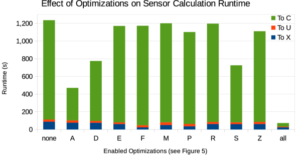
Figure 7: Runtime of Figure 5’s PLara plan with different optimizations enabled on one month’s data from two sensors. We decompose runtimes for Figure 5 into the portion scanning $A$ and $B$ to calculating $X$, from $X$ to $U$, and from $U$ to $C$; the $C$ calculation dominates runtime.

5.2 Competitiveness Experiment

In this section we conduct an experiment to test whether LaraDB competes in performance with the analytics engine natively integrated with Accumulo: MapReduce.

The task we run is matrix multiplication (MxM). In terms of RA, MxM consists of a join followed by an aggregation. In terms of LA, many other LA kernels can be simulated by MxM. For example, matrix reduction can be realized as multiplication by a vector of 1s, and matrix subset can be realized as multiplication on the left by a diagonal matrix that selects rows and on the right by a diagonal matrix that selects columns. Composition of these kernels lead to more complex graph algorithms such as triangle enumeration [33], vertex similarity, k-truss, and matrix factorization [15].

Because our goal is to compare the performance of the LaraDB and the MapReduce execution engines, rather than the difference between two MxM algorithms, we wrote the LaraDB and MapReduce code implementing MxM as similarly as possible. Both read inputs from and write outputs to Accumulo tables. Both implement the the MxM $C=AB$ outer product algorithm [20] on pre-indexed data with $A$ sorted column-major and $B$ sorted row-major. Both have optimizations (A) and (D) from Section 4.2 enabled.

The main operational difference between the LaraDB and MapReduce execution is that LaraDB executes inside Accumulo’s range scan iterators while MapReduce executes as external processes managed by the YARN scheduler. Specifically, MapReduce performs a reduce-side join [13].

We generated test data via the Graph500 unpermuted power law graph generator [4]. We chose the generator because power law distributions well model properties of real world data such as skew [17]. Generated matrices range from $2^{10}$ rows (scale 10) to $2^{19}$ rows (scale 19), each with roughly 16 nonzero entries per row. Multiplying the largest matrices formed close to $2^{33}$ ($=8\times 10^{9}$) partial products.

We used the same Amazon EC2 experiment environment as Section 5.1, except with 8 workers instead of 4. Each worker allocated 3 GB of memory to YARN and 3 GB to Accumulo. The 8-worker environment is well-suited to gauging inter-node parallelism; intra-node parallelism, however, was limited by the small number of vCPUs (2) per machine.

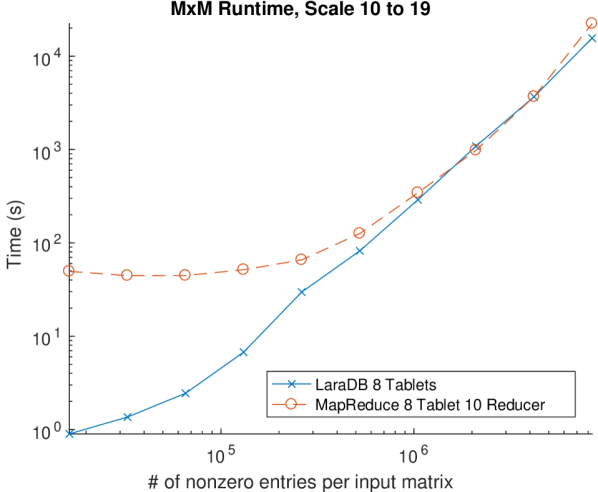
Figure 8: 8-worker $A^{\intercal}B$ experiment runtime as problem size increases. LaraDB dominates at smaller sizes, while LaraDB and MapReduce converge at larger sizes.

Figure 8 plots MxM runtime as problem size increases. Graphulo dominates MapReduce at smaller problem sizes. This is due to the large startup cost that MapReduce programs are infamous for; the YARN scheduler takes roughly 30s to start any task as a result of job submission, container allocation, jar copying, and other cold start overheads.

LaraDB, on the other hand, has a warm start since it runs inside the already-running Accumulo tablet servers. These tablet servers have a standing thread pool ready to service scan requests as soon as they receive a remote procedure call. We conclude that LaraDB is much better suited to interactive and small-scale computation, such as analytics on a subset of data extracted from an Accumulo table.

At larger problem sizes, LaraDB and MapReduce converge in performance. The convergence meets our expectations because the two libraries run similar code in a similar pattern of parallelism over the same data partitioning. Their execution environment, JVMs over Hadoop, is also similar given sufficient time to amortize YARN’s startup cost.

We conclude that our LaraDB implementation is competitive with at least one major RA/LA system at scale. We take this as initial evidence that systems built atop the Lara algebra can and do have strong performance.

6 Conclusion

Linear algebra (LA) and relational algebra (RA) are, in a sense, two sides of the same coin. We offer Lara as that coin, expressive enough to subsume LA and RA yet with more structure than MapReduce that in turn affords greater reasoning. Lowering Lara to a physical algebra brings this reasoning to the domain of partitioned sorted maps, a broad abstraction that encompasses LA, RA, and key-value systems including the LaraDB implementation on Accumulo.

Our experiments demonstrate that (1) Lara expresses high and low-level optimizations that make a difference in the execution of real-world tasks, and (2) that the LaraDB implementation outperforms an existing data processing system vastly at small scale and competitively at large scale.

In the future, we aim to use Lara as a conduit for studying and computationally exploiting the relationship between LA and RA. A database optimizer is an ideal place to realize the benefits of this study for joint linear-relational analytics.

References

- [1] S. M. Aji and R. McEliece. The generalized distributive law. Transactions on Information Theory, 46(2):325–343, 2000.
- [2] A. Alexandrov, R. Bergmann, S. Ewen, J.-C. Freytag, F. Hueske, A. Heise, O. Kao, M. Leich, U. Leser, V. Markl, et al. The stratosphere platform for big data analytics. The VLDB Journal, 23(6):939–964, 2014.
- [3] Array of things. https://arrayofthings.github.io/.
- [4] D. Bader, K. Madduri, J. Gilbert, V. Shah, J. Kepner, T. Meuse, and A. Krishnamurthy. Designing scalable synthetic compact applications for benchmarking high productivity computing systems. Cyberinfrastructure Technology Watch, 2:1–10, 2006.
- [5] Y. Bu, B. Howe, M. Balazinska, and M. D. Ernst. The HaLoop approach to large-scale iterative data analysis. VLDB Journal, 21(2):169–190, 2012.
- [6] A. Buluc and J. R. Gilbert. On the representation and multiplication of hypersparse matrices. In International Symposium on Parallel and Distributed Processing (IPDPS). IEEE, 2008.
- [7] P. Buneman, S. Naqvi, V. Tannen, and L. Wong. Principles of programming with complex objects and collection types. Theoretical Computer Science, 149(1):3–48, 1995.
- [8] R. Chaiken, B. Jenkins, P.-Å. Larson, B. Ramsey, D. Shakib, S. Weaver, and J. Zhou. Scope: easy and efficient parallel processing of massive data sets. Proceedings of the VLDB Endowment, 1(2), 2008.
- [9] F. Chang, J. Dean, S. Ghemawat, W. C. Hsieh, D. A. Wallach, M. Burrows, T. Chandra, A. Fikes, and R. E. Gruber. Bigtable: A distributed storage system for structured data. ACM Transactions on Computer Systems (TOCS), 26(2):4, 2008.
- [10] B. Chattopadhyay, L. Lin, W. Liu, S. Mittal, P. Aragonda, V. Lychagina, Y. Kwon, and M. Wong. Tenzing a SQL implementation on the mapreduce framework. PVLDB, 4:1318–1327, 2011.
- [11] A. Crotty, A. Galakatos, K. Dursun, T. Kraska, U. Cetintemel, and S. B. Zdonik. Tupleware: “big” data, big analytics, small clusters. In Conference on Innovative Data Systems Research (CIDR), 2015.
- [12] T. Elgamal, S. Luo, M. Boehm, A. V. Evfimievski, S. Tatikonda, B. Reinwald, and P. Sen. Spoof: Sum-product optimization and operator fusion for large-scale machine learning. In Conference on Innovative Data Systems Research (CIDR), Jan. 2017.
- [13] L. Fegaras, C. Li, and U. Gupta. An optimization framework for map-reduce queries. In EDBT. ACM, 2012.
- [14] Apache flume. https://flume.apache.org/.
- [15] V. Gadepally, J. Bolewski, D. Hook, D. Hutchison, B. Miller, and J. Kepner. Graphulo: Linear algebra graph kernels for NoSQL databases. In International Parallel & Distributed Processing Symposium Workshops. IEEE, 2015.
- [16] V. Gadepally and J. Kepner. Big data dimensional analysis. In High Performance Extreme Computing Conference (HPEC). IEEE, 2014.
- [17] V. Gadepally and J. Kepner. Using a power law distribution to describe big data. In High Performance Extreme Computing Conference (HPEC). IEEE, 2015.
- [18] J. M. Hellerstein, C. Ré, F. Schoppmann, D. Z. Wang, E. Fratkin, A. Gorajek, K. S. Ng, C. Welton, X. Feng, K. Li, et al. The madlib analytics library: or mad skills, the sql. Proceedings of the VLDB Endowment, 5(12):1700–1711, 2012.
- [19] D. Hutchison, B. Howe, and D. Suciu. Lara: A key-value algebra underlying arrays and relations. arXiv preprint arXiv:1604.03607, 2016.
- [20] D. Hutchison, J. Kepner, V. Gadepally, and A. Fuchs. Graphulo implementation of server-side sparse matrix multiply in the Accumulo database. In High Performance Extreme Computing Conference (HPEC). IEEE, 9 2015.
- [21] D. Hutchison, J. Kepner, V. Gadepally, and B. Howe. From NoSQL Accumulo to NewSQL Graphulo: Design and utility of graph algorithms inside a BigTable database. In High Performance Extreme Computing Conference (HPEC). IEEE, 9 2016.
- [22] J. Kepner, P. Aaltonen, D. Bader, A. Buluç, F. Franchetti, J. Gilbert, D. Hutchison, M. Kumar, A. Lumsdaine, H. Meyerhenke, S. McMillan, J. Moreira, J. D. Owens, C. Yang, M. Zalewski, and T. Mattson. Mathematical foundations of the GraphBLAS. In HPEC. IEEE, 9 2016.
- [23] J. Kepner, V. Gadepally, D. Hutchison, H. Jananthan, T. Mattson, S. Samsi, and A. Reuther. Associative array model of SQL, NoSQL, and NewSQL databases. In High Performance Extreme Computing Conference (HPEC). IEEE, 9 2016.
- [24] A. Kunft, A. Alexandrov, A. Katsifodimos, and V. Markl. Bridging the gap: towards optimization across linear and relational algebra. In Proceedings of the 3rd SIGMOD Workshop on Algorithms and Systems for MapReduce and Beyond. ACM, 2016.
- [25] R. Maas, J. Hyrkas, O. G. Telford, M. Balazinska, A. Connolly, and B. Howe. Gaussian mixture models use-case: in-memory analysis with myria. In Proceedings of the 3rd VLDB Workshop on In-Memory Data Mangement and Analytics. ACM, 2015.
- [26] B. Marker, M. Schatz, D. Matthews, I. Dillig, R. van de Geijn, and D. Batory. Dxter: An extensible tool for optimal dataflow program generation. Technical report, Technical Report TR-15-03, The University of Texas at Austin, 2015.
- [27] X. Meng, J. Bradley, B. Yavuz, E. Sparks, S. Venkataraman, D. Liu, J. Freeman, D. Tsai, M. Amde, S. Owen, et al. Mllib: Machine learning in apache spark. Journal of Machine Learning Research, 17(34):1–7, 2016.
- [28] S. Palkar, J. J. Thomas, A. Shanbhag, D. Narayanan, H. Pirk, M. Schwarzkopf, S. Amarasinghe, M. Zaharia, and S. InfoLab. Weld: A common runtime for high performance data analytics. In Conference on Innovative Data Systems Research (CIDR), Jan. 2017.
- [29] A. Rheinländer, A. Heise, F. Hueske, U. Leser, and F. Naumann. SOFA: An extensible logical optimizer for udf-heavy data flows. Information Systems, 52, 2015.
- [30] D. Shukla, S. Thota, K. Raman, M. Gajendran, A. Shah, S. Ziuzin, K. Sundaram, M. G. Guajardo, A. Wawrzyniak, S. Boshra, R. Ferreira, M. Nassar, M. Koltachev, J. Huang, S. Sengupta, J. J. Levandoski, and D. B. Lomet. Schema-agnostic indexing with azure documentdb. PVLDB, 8:1668–1679, 2015.
- [31] M. Spight and V. Tropashko. First steps in relational lattice. arXiv preprint cs/0603044, 2006.
- [32] J. Wang, T. Baker, M. Balazinska, D. Halperin, B. Haynes, B. Howe, D. Hutchison, S. Jain, R. Maas, P. Mehta, et al. The Myria big data management and analytics system and cloud service. Jan. 2017.
- [33] M. M. Wolf, J. W. Berry, and D. T. Stark. A task-based linear algebra building blocks approach for scalable graph analytics. In High Performance Extreme Computing Conference (HPEC). IEEE, 2015.
- [34] M. Zaharia, M. Chowdhury, M. J. Franklin, S. Shenker, and I. Stoica. Spark: cluster computing with working sets. HotCloud, 10:10–10, 2010.