Deep Learning for Explicitly Modeling
Optimization Landscapes

Abstract

In all but the most trivial optimization problems, the structure of the solutions exhibit complex interdependencies between the input parameters. Decades of research with stochastic search techniques has shown the benefit of explicitly modeling the interactions between sets of parameters and the overall quality of the solutions discovered. We demonstrate a novel method, based on learning deep networks, to model the global landscapes of optimization problems. To represent the search space concisely and accurately, the deep networks must encode information about the underlying parameter interactions and their contributions to the quality of the solution. Once the networks are trained, the networks are probed to reveal parameter combinations with high expected performance with respect to the optimization task. These estimates are used to initialize fast, randomized, local search algorithms, which in turn expose more information about the search space that is subsequently used to refine the models. We demonstrate the technique on multiple optimization problems that have arisen in a variety of real-world domains, including: packing, graphics, job scheduling, layout and compression. The problems include combinatoric search spaces, discontinuous and highly non-linear spaces, and span binary, higher-cardinality discrete, as well as continuous parameters. Strengths, limitations, and extensions of the approach are extensively discussed and demonstrated.

1 Introduction to Optimization via Search Space Modeling

In the 1990s, a number of researchers [1] [2] [3] [4] independently started employing probabilistic models to guide heuristic stochastic based-search algorithms. The idea was simple, to use the knowledge of the search landscape that may be ascertained by analyzing the points encountered to guide where to look next. This sharply contrasted the procedure of many successful randomized hill-climbing algorithms that made small perturbations stochastically in hopes that a better solution was a close neighbor to the current best solution.

In the simplest instantiation, probabilistic methods explicitly maintain statistics about the search space by creating models of the good solutions found so far. These models are then sampled to generate the next query points to be evaluated. The sampled solutions are then used to update the model, and the cycle is continued. Probabilistic models for optimization were motivated with three goals: as a new optimization method, as a method to incorporate simple learning (Hebbian style probability updates) into hillclimbing, and as a method to explain how genetic algorithms  [5] [6] [7] might work.

A bit more detail on the third motivation is warranted: by maintaining a population of points (rather than a single point from which search is centered), genetic algorithms (GAs) can be viewed as creating implicit probabilistic models of the solutions seen in the search. GAs attempt to implicitly capture dependencies between parameters and solution quality through the distribution of parameter settings contained in the population of solutions. Exploration proceeds by generating new samples to evaluate through a process of applying randomized “recombination/crossover” operators to pairs of high-performance members of the population. Because only the high-performance are selected for recombination, parameter settings found in the poor-performing solutions are not explored further. The recombination operator, which combines two “parents” candidate solutions by producing “children” that transfer sets of parameters from each parent into the children, serves to keep sets of parameters together (though in a randomized manner) in the next set of candidate solutions that are explored. In terms of sampling, this can be viewed as a simple approach to sampling the population’s statistics. Though similar in intent, this implicit manner of sampling the distribution of solutions contrasts with the approach presented in this paper. Here, explicit steps are taken to model the parameters interdependencies that contribute to the quality of candidate solutions. The goal of this paper is succinctly stated as follows:

The primary goal of this paper is to demonstrate that while employing any search algorithm (hillclimbing, GA, simulated annealing, etc.), it is possible to simultaneously learn a deep-neural network based approximation of the evaluation function. Then, through the use of “deep-network inversion” (employed as a method to sample the deep networks), intelligent perturbations of some/all of the samples generated by the search algorithm can be made. After these perturbations, the the new solutions should have an increased probability of higher scores. As a secondary benefit, this modeling may also be used to make the evaluation more efficient by replacing it with the DNN’s approximation of the evaluation function.

1.1 Predecessors to Deep Modeling of Optimization Landscapes

Within the GA literature, one of the first attempts at using population level statistics was the “Bit-Based Simulated Crossover (BSC)” operator [8]. Instead of combining pairs of solutions, population-level statistics were used to generate new solutions. The BSC operator worked as follows. For each bit position, the number of population members which contain a one in that bit position were counted. Each member’s contribution was weighted by its fitness with respect to the target optimization function. The same process was used to count the number of zeros. Instead of using traditional crossover operators to generate new solutions, BSC generated new query points by stochastically assigning each bit’s value by the probability of having seen that value in the previous population (the value specified by the weighted count). The important point to note is that BSC used the population statistics to generate new solutions.

Extending the above idea and incorporating Hebbian learning, another early probabilistic optimization was the Population-Based Incremental Learning algorithm (PBIL) [1]. Rather than being based on population-genetics, the lineage for PBIL stems back to early reinforcement learning. PBIL is akin to a cooperative system of discrete learning automata in which the automata choose their actions independently, but all automata receive a common reinforcement dependent upon all their actions [9]. Unlike most previous studies of learning automata, which have commonly addressed optimization in noisy but very small environments, PBIL was used to explore large deterministic spaces.

The PBIL algorithm, most easily described with a binary alphabet, works as follows. The algorithm maintains a real-valued probability vector, specifying the probability of generating a 1 or a 0 in each bit position (just the first order statistics). The probability vector is sampled repeatedly to generate a set of new candidate solutions. These candidates are evaluated with respect to the optimization function, and the best solution is kept and all the other discarded. The probability vector is “moved” towards the best solution through simple Hebbian-like updates. And the cycle is repeated. Note that the probabilistic model created in PBIL is extremely simple: There are no inter-parameter dependencies captured; each bit is modeled independently. The entire probability model is a single vector. Although this simple probabilistic model was used, PBIL was successful when compared to a variety of standard genetic algorithm and hillclimbing procedures on numerous benchmark and real-world problems. A more theoretical analysis of PBIL can be found in [2][10][11][12][13][14].

The most immediate improvements to PBIL are mechanisms that capture inter-parameter dependencies. Mutual Information Maximization for Input Clustering (MIMIC) [15] was one of the first to do this. MIMIC captured a heuristically chosen set of the pairwise dependencies between the solution parameters. From the top N% of all previously generated solutions, pair-wise conditional probabilities were calculated. MIMIC then used a greedy search to generate a chain in which each variable was conditioned on the previous variable. The first variable in the chain, $X_{1}$, was chosen to be the variable with the lowest unconditional entropy, $H(X_{1})$. When deciding which subsequent variable, $X_{i+1}$, to add to the chain, MIMIC selected the variable with the lowest conditional entropy, $H(X_{i+1}|X_{i})$. This extended the solely-unconditional model with PBIL to maintain a set of pair-wise dependencies. In [16], MIMIC’s probabilistic model was extended to a larger class of dependency graphs: trees in which each variable is conditioned on at most one parent. As shown in 1968, this created the optimal tree-shaped network for a maximum-likelihood model of the data  [17]. In experimental comparisons, MIMIC’s chain-based probabilistic models typically performed significantly better than PBIL’s simpler models. The tree-based graphs performed significantly better than MIMIC’s chains.

The trend indicated that more accurate probabilistic models increased the probability of generating new candidate solutions in promising regions of the search space [18]. The natural extension to pair-wise modeling is modeling arbitrary dependencies. Bayesian networks are a popular method for efficiently representing dependencies [19] [20]. Bayesian networks are directed acyclic graphs in which each variable is represented by a vertex, and dependencies between variables are encoded as edges. Numerous researchers have taken the step of combining full Bayesian networks with stochastic search  [21] [22] [23]. For an overview, see  [24].

An alternate model building approach, termed STAGE, was presented in [25]. STAGE attempts to map a set of user-supplied features of the state space to a single value. This value represents the quality of solutions found thus far. The “value function” is used to select the next point from which to initialize search. Unlike the other algorithms described above, which attempt to automatically model the effects of parameter combinations on the overall solution quality, here hand-created features related to the optimization function are used. Other than the use of hand-crafted features, this approaches shares many of the important characteristics of the methods used in this paper.

In the next section, we describe the Deep-Opt algorithm and give details of how the probabilistic model is created and sampled. We also describe how the model is integrated with fast-search heuristics, following the work of [25] and [16]. In Section 3, we examine the performance of Deep-Opt on a wide variety of test problems. There are many interesting alternatives and extensions to the approach used here; experiments with three are presented in Section 4. The three alternatives help to increase the set of problems that can be tackled and address some of the limits of the approach as described in Section 2. Finally, a discussion of the results and suggestions for future work are presented in Section 5.

2 Deep Learning for Search Space Modeling

Optimization with probabilistic modeling, at a high level, is simply explained in Figure 1. As shown in the figure, in previous work, we started with a large set of candidate solutions and evaluated them with respect to the objective function of the problem to be solved (e.g. the total tour length of the classic traveling salesman problem). The poor-performing candidate solutions were discarded. The set of remaining solutions, usually a small subset of the better performing members from the original set, were then modeled. The model was stochastically sampled, the solutions evaluated, and the process was continued.

Algorithm 1 High Level Probabilistic Modeling for Optimization Create set, S, with random solutions from uniform distribution. while termination condition is not met do      Create a probabilistic model, PM, of S.      Stochastically sample from PM, to generate C candidate solutions.      Evaluate the C candidate solutions.      Update S with only the N high-evaluation solutions from $C$, where $N\ll C$.

Figure 1: Probabilistic Modeling for Optimization Overview.

In the interest of being concrete, a simple example of a probabilistic model is provided in Figure 2 using PBIL’s independent-parameter model to represent 4 different populations . Once the model, $PM$, is created, $PM$ is sampled to generate the candidate solutions to evaluate next. Why does this idea work? The solutions that are represented in $PM$ are only those with high evaluations (the poor performing ones were discarded and never modeled), therefore, those that are subsequently generated by sampling the statistics of multiple good solutions should be high-performing as well. A large number of solutions are generated, each is evaluated, and the lower-performing ones discarded, and the procedure is repeated .

Population A: 1000
0010
1000
1001
— 0.75, 0.00, 0.25, 0.25 Population B: 1010
1010
0101
0101
— 0.50, 0.50 0.50, 0.50 Population C: 1000
0010
0000
0000
— 0.25,0.00,0.25,0.00 Population D: 1111
0000
1111
0000
— 0.50, 0.50 0.50, 0.50

Figure 2: Modeling 4 different binary-populations of 4 samples each. In PBIL’s probabilistic model, each bit position is modeled independently and is simply the probability of having a ’1’ in each bit position. This distribution can easily be sampled to generate new points to evaluate.

Note that although PBIL’s probabilistic model is extremely simple, and no inter-parameter dependencies are modeled, as mentioned earlier, even this proved effective in many standard optimization tasks. Despite the successes, however, as shown in Figure 2 there are severe limitations: population sets B & D, although different, are represented with the same probabilistic vector; thereby demonstrating the inadequacy of the models and the need for more powerful representations of the candidate solution’s statistics. Thus, models such as MIMIC & Optimal-Dependency-Trees (described in Section 1), in which pair-wise or higher-order dependencies were represented, were introduced. As problem complexity increased, these more flexible and powerful models improved the quality of the solutions generated.

In this paper, we use a neural network to create a mapping between the solutions sampled to that point and their score, as determined by the evaluation function. In the context of describing the algorithm, we also expose four of the largest differences between our approach and the approaches used earlier.

(1)

One of the primary differences is that by using a deep neural network, we do not a priori specify the form of the dependencies in the probabilistic model (e.g. pair-wise, or triplet combinations, etc.) Although the architecture of the neural network used for modeling is manually specified, the actual dependencies that the network encodes need not be the same form for all parameters, nor are they deeply tied to architecture of the network [26]. For all but one of the tests described in this paper, the neural network architecture will not change; a deep network is capable of modeling the necessary statistics.

(2)

Once the network has learned the mapping from input parameters to evaluation, a procedure for generating the new points to evaluate is necessary. This procedure is quite different than the straight-forward sampling that was possible in the previous models such as those in PBIL or dependency trees. In the simplest model, PBIL (see Figure 2), samples were easily generated by a biased-random sample, where a ’1’ was generated in position $p$ independently from any other bit, as specified by the real-value in position $p$ in the probability vector. With models with dependencies, such as the dependency-trees [17], the sampling is simply conditioned on the variables on which the parameter is dependent (as specified in the tree-based model).

With neural networks, however, generating samples is more complex. It is based on the technique of “network inversion”: given a trained network, network inversion uses standard back-propagation to  modify the inputs rather than the network’s weights. The inputs are modified to match the preset and clamped outputs. This method was first presented in [27] and has recently been popularized within the context of texture and style generation with neural networks  [28] [29].

We use it as follows: We are given a trained network that maps the input parameters (scaled between 0.0 and 1.0) to their evaluation (also scaled between 0.0 and 1.0). First, all the weights of the network are frozen; they will not change for the sample generation process. Second, we clamp the output to the desired output — for maximization problems, we clamp the output 1.0; this indicates that we would like to generate solutions that are as good as the best ones seen so far.

The inputs are then initialized (either randomly or by other means such as perturbing the best solution seen thus far) and the network performs a forward propagation step and the error is measured at the output. The error metric is the standard Least-Mean Squares Error on the target output (which is clamped to 1.0).

$$E_{LMS}=\sum_{i\in outputs}(targets_{i}-predicted_{i})^{2}$$

Since we pin the target to 1.0, and there is only a single output scaled between 0.0 and 1.0 (that represents the score of the candidate solution). This is simply:

$$E_{LMS}=(1.0-predicted_{score})^{2}$$

A process similar to standard training with stochastic-descent back-propagation (or any other network training procedure) is then used. However, unlike standard training, the errors are propagated all the way back to the inputs, and the inputs are modified – not the weights. As described in [27], the procedure addresses the following question: “Which input should be fed into the net to produce an output which approximates the given target vector T’ (in our case the the target vector T is a simple scalar of 1.0). The error signal for the input $i$:

$$\delta_{i}=-\dfrac{\delta E}{\delta input_{i}}$$

tells the input units how to change (direction and magnitude) to decrease the error . In general, modest learning-rates for the gradient descent algorithm were found to work best for the network-inversion process (we used the Adam Optimizer [30] with learning-rate = 0.001). If the networks are trained well such that they successfully model the search landscape, then the set of input values found through this procedure will yield high-evaluation solutions when tested on the actual evaluation function.

(3)

Once the new candidate solutions are generated and evaluated, what is the next step? In the previous uses of probabilistic models (Figure 1), the low-performance candidate solutions were discarded and the high-performance solutions were kept. Interestingly, the actual evaluation of the high-performance solutions was not used. In contrast, in our procedure, we create an explicit mapping from the candidate solution to its score . This reflects a fundamental difference in approaches: since an explicit mapping is created, it is not assumed that the model only represents good solutions; it represents both high and low quality solutions.

(4)

Finally, note that in contrast to many previous studies that represented the solution vectors as binary strings and modeled only the binary parameters, the deep-neural networks used in this study naturally model real-values. Extensions to binary and other discrete parameters will be described in Section 4.

Algorithm 2 Next-Ascent Stochastic Hillclimbing (NASH) (shown for maximization) Create a random candidate solution, $c$, composed of $|P|$ real-valued parameters. BestEvaluation $\leftarrow$ Evaluate ($c$) while termination condition is not met do      $c^{\prime}\leftarrow c$      Number-Perturbations = Select-Random-Integer from $[1,m\times|c|]$      loop Number-Perturbations          Randomly select a parameter, $p$, from $c^{\prime}$          c’ $\leftarrow$ Modify $p$ to a randomly chosen value between $[(0.75*p),(1.25*p)]$            CandidateEvaluation $\leftarrow$ Evaluate (c’)      if (CandidateEvaluation $\geq$ BestEvaluation) then          $c\leftarrow c^{\prime}$          BestEvaluation $\leftarrow$ CandidateEvaluation      else          Discard $c^{\prime}$       Return c

Figure 3: Next-Ascent Stochastic Hillclimbing (NASH). In our implementation we set $m=2\%$. Note that the mutation amount $\pm 0.25$ is quite large; however, this was set based on extensive empirical testing on these and similar problems. |P| is dependent on the problem. In the experiments presented throughout this paper, it ranged from 50 to 1600.

2.1 Integration with Fast Local Search Heuristics

In the simplest implementation, the candidate solutions generated by the network inversion are evaluated and the cycle is continued. Although this method will work, there are drawbacks. First, this is a slow process; training a full network to map the sampled points to their evaluations is an expensive procedure, as is sampling the network. Second, a post-processing step of local optimization, where small changes are made to the solutions generated, yields improvement to the solutions found. This is because both the interpolation and extrapolation capabilities of the trained networks are not perfect; there will be discrepancies between the estimated “goodness” (evaluation) of a candidate solution and its actual evaluation.

Two early works in probabilistic model-based optimization [16] [25] suggested the use of the probabilistic models as methods to initialize faster local-search optimization techniques. This technique is used here. A very simple next-ascent stochastic hillclimbing (NASH) procedure is shown in Figure 3. It has repeatedly proven to work well in practice when used in conjunction with other optimization algorithms to perform local optimization, and also surprisingly well when used alone in a variety of scenarios  [31] [32] [33] [34]. For the majority of the paper, we will use NASH as the underlying search process; the neural modeling will “wrap-around” NASH.

Importantly, note that NASH is initialized with a single candidate solution. This candidate is perturbed until an equal or better solution is found. This fits well into the procedures described thus far: all of the candidate solutions evaluated by NASH can be added to the pool of solutions to be modeled, $S$. When the networks are trained and a next set of candidate solutions are generated, the single best solution from them is used to initialize the NASH algorithm. NASH proceeds as normal, again recording all the candidate solutions it evaluates – which are then use to augment $S$ in the next time step, and the cycle continues.

A visual description of the algorithm is shown in Figure 4.

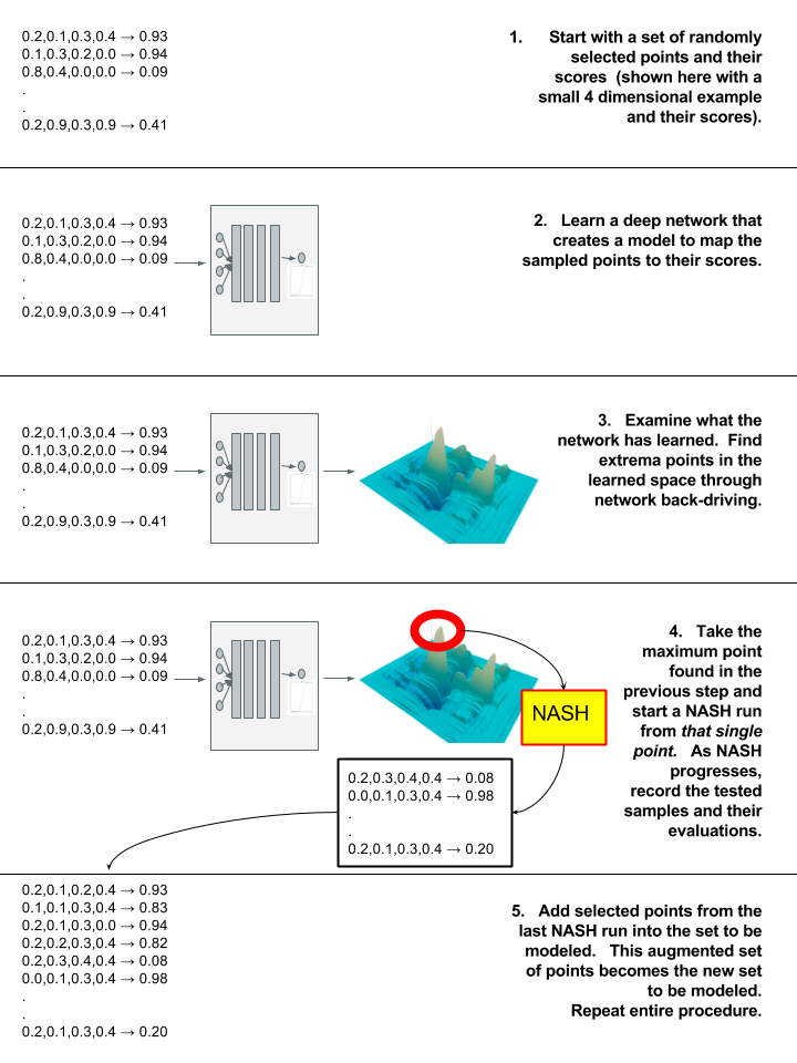
Figure 4: A visual description of Deep-Opt. (Sample topographic plot by [35])

2.2 Putting it all Together

In this section, we describe some of the pragmatic considerations for deployment, and put all of the steps into step-by-step directions.

There are many possible ways to create and maintain $S$, the samples that are used for training the modeling networks. In our study, the size of S is kept constant throughout the run. Although a sufficiently large deep neural network should be able to represent the surface represented by all of the points seen, it would require both extra computation and not be valuable in practice. Overly precise models of low-evaluation areas are not necessary. To keep $S$ a constant size, after every NASH run, the last 1000 unique solutions from the NASH run are added to $S$, and $S$ is pruned back by removing the members that have been in S the longest (this implements a simple first-in-first-out scheme), as was suggested in previous studies [16]. If the algorithm is progressing correctly, the average score of the solutions present in $S$ increases over time.

The full Deep-Opt algorithm is shown in Figure 5. With respect to the step “Train a Deep Neural Network”, there are several points that should be noted. The use of a validation set is vital to good performance. In each training cycle, (100) samples are drawn by perturbing the best solution and added to the validation set. Then, after each step in training, the correlation between the actual evaluation of these samples and the network’s predicted evaluation of these samples is measured. When the correlation begins to decrease, training is stopped and the next step of the algorithm begins. If the correlation is negative, training is restarted with random weights.

Algorithm 3 Deep-Opt at a High-Level 1: 2:Create set, S, with candidate solutions from uniform distribution. 3:Evaluate all solutions in S. 4: 5:while termination condition is not met do 6:     Scale all real evaluations of $s$ to range [0.0,1.0], $\forall(s|s\in S)$ 7:     Train a Deep Neural Network (DNN) to map $s\rightarrow Evaluation(s),\forall(s|s\in S)$ 8:     Freeze the weights of the deep network. 9: 10:     $\triangleright$ Stochastically Generate New Candidates 11:     Initialize $C$ to be empty. 12:     repeat 13:         Generate a new candidate solution, $c$, by randomly perturbing the best solution found so far 14:         Append $c$ to $C$.    $C\leftarrow C+c$ 15:     until (|C| = Number-To-Generate-From-Model) 16: 17:     $\triangleright$ Back-Drive the Network to Improve Some of the Generated Samples 18:     Select a fraction, $F$, of the members of $C\rightarrow C^{\prime},s.t.|C^{\prime}|\leq|C|$. 19:     Clamp the network’s output to 1.0 20:     for each $d\in C^{\prime}$ do 21:         Initialize the inputs of the DNN with $d$ 22:         Back-Drive the network until the inputs stop changing $\rightarrow d^{\prime}$ 23:         Replace $d$ in C with $d^{\prime}$       24: 25:     Evaluate all candidates, $c\in C$. 26: 27:     $\triangleright$ Run the local optimization 28:     Select a single candidate, $m$ ($m\in C$), where $m$ is has the highest evaluation of all in $C$. 29:     Initialize NASH with $m$. 30:     Run NASH and record all of the unique solutions (into set $Y$) evaluated by the NASH run. 31: 32:     $\triangleright$ Update the data to be modeled 33:     $Y^{\prime}\leftarrow$ Select a subset of the best solutions from $Y$. 34:     $S\leftarrow S+Y^{\prime}$ 35:     Discard Duplicates in $S$; prune $S$ if necessary 36:

Figure 5: Deep-opt: Creating a model of the search landscape to initialize fast search algorithms (NASH). We set the Number-to-Generate-From-Model = 50 for all of our tests. $|S|$ was kept at 10,000 samples with the size of $Y^{\prime}$ set at 1000. For simplicity, $F$ was kept static at 50% for all of the tests in this paper.

There are two implementation details not specified in Figure 5. In the first step, Line 1, several variants of creating the initial set, $S$, are possible. The simplest is, as shown, generating samples entirely randomly. Fully random sampling gives the broadest exploration of the search space. Alternatively, we could have performed a single NASH run and saved all the points explored. Using only one run, however, gives a poor representation of the global landscape because only a deep, single, path is explored. A third alternative is to sample a number of seed-points randomly and also explore their local neighborhoods by making small perturbations of the seed points. This gives a cursory indication of the local landscape around each of the seed points; empirically, this improved results on the problems tested. We use this initialization method throughout the paper. A full analysis was not conducted to measure the effects of alternate approaches.

Second, as can be seen, there are a large number of parameters and decisions made in the algorithm design. Our goal is to show that using a deep neural network is capable of modeling the search space, not necessarily advocating a particular network or set of parameters. Nonetheless, to make the study complete, we need to specify the networks we used. For the trials in this paper, two networks were used. The first, Deep-Opt-5, used a 5-fully-connected-layer network with 100 hidden units per layer. The second, Deep-Opt-10 used a 10-layer fully-connected network with 20 hidden units per layer and skip connections between every layer and its predecessors. Both networks have a single output - the estimate of the evaluation of the function being estimated. Weight decay was used in training (0.98). A variety of networks were tried, ranging from simple single layer networks to even deeper ones. As expected, the best performer was dependent on the problem, however these provided good results across multiple problems.

Finally, the very careful reader may have noted that the effort to separate the steps in Lines 8-11 from those in lines 13-19. Later in the paper, we will show how lines 8-11 can be replaced with other procedures.

2.3 Visualizing the Learning

Before turning our attention to the empirical tests in the next section, we present a motivating example to demonstrate how the local search algorithms utilize the models created. We examine a simple problem in which the evaluation is: $evaluation(\boldsymbol{x})=\sum_{i=1}^{50}(x_{i}*sin(x_{i}))$. We instantiate this problem with 50 parameters that can take on values between [0,100]. Note that in this maximization problem, each parameter is independent. Though this is trivial problem, it serves to demonstrate the expected behavior.

If a NASH search is initialized with a solution vector that has low values for any of the parameters, there are many local optima on the way to the global optima. Nonetheless, because of the ease of the problem, even with no learning, some of the runs will find the global optima.

In Figure 6 (top-row), in the left column are the starting points for all 50 of the parameters before the NASH algorithm is run. As expected, they are randomly distributed across the input range. By the end of the NASH run (right column) many of the parameters are close to their optimal settings.

The middle row of Figure 6 shows the same (start/end configurations) for the 10th restart of NASH. Because NASH is still initialized randomly (no learning), we expect to see largely the same distribution of points in the beginning and the end. The same is shown in the bottom row, the 25th restart of NASH.

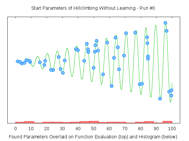
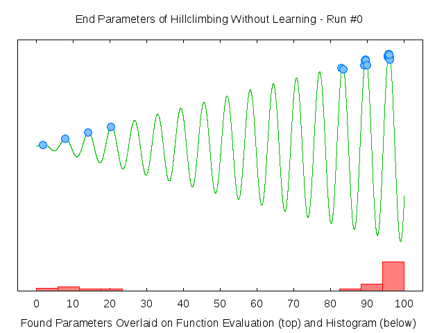
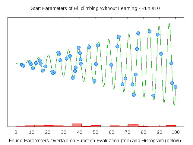
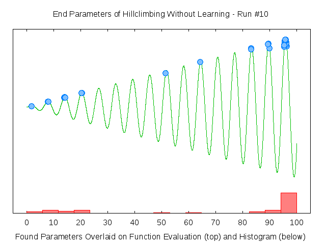
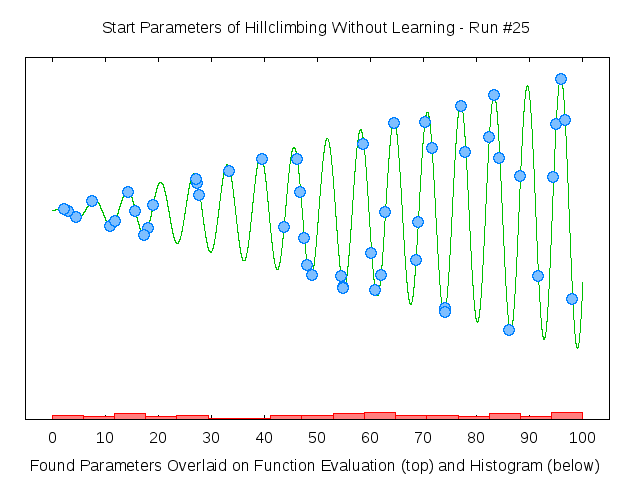
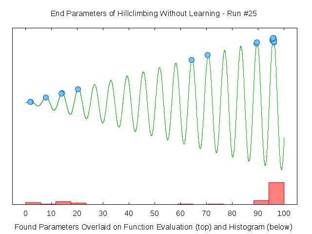
Figure 6: Sines Problem without Learning. The (green) line is the underlying function to be maximized. The (blue) points are the settings of each the 50 parameters in the beginning (left) and ending (right) of the NASH procedure (random perturbations of best seen-so-far). A histogram showing the distribution of the points is shown in red (this is shown because of the difficulty in seeing the overlapping points in this graph). Note that in the beginning of each run (left column), the points are uniformly distributed across the full input space. The results have vastly improved through hillclimbing, though not all points have made it to the global optimum. Top Row: NASH run #1, Middle Row: NASH run #10 (this is the HC run made after the 9th modeling step), Bottom Row: NASH run #25. Note about the graph: although each points represents one of the 50 parameters in the same single solution string, they are shown ’folded-over’ onto the same graph. This is possible because each parameter is independent and is evaluated with respect to the same function.

Next, we repeat the same experiment with Deep-Opt. The only difference is in the initialization of the NASH algorithm. The samples that are generated in each NASH run are added to the set of solutions that are modeled by the neural network. From this neural network model, $M$ new samples are drawn. The single best of the $M$ is used to initialize the next NASH run. As expected, in Figure 7, the first run looks similar to the earlier case with no model. This is because there is no information in the model as yet. However, after the 10th NASH restart, (middle-row, Figure 7) there is a distinct difference in the starting values – many more are already in high-evaluation regions. The best solution found through sampling had many of its parameters in the right region of the search space. The likelihood of these reaching the global optimum is increased through NASH (right column). By the 25th run, this trend is even further evident. Sampling the model works as expected: the starting point for the hillclimbing is already in a better region - where more parameters are closer to the global optima.

Though this problem is simple, it demonstrates how the modeling can improve the search results. Interestingly, early on in our studies, modeling sometimes led to poorer overall performance. Why? As the probabilistic model improved, exploration decreased – more samples started in a basin of attraction that led to the same local maxima as was seen previously. Improvement slowed because the updates to the model all happened with similar candidate solutions. The algorithm parameters, in particular the size of the sample set that was used for modeling, $|S|$, were tuned to the settings shown in Figure 5 to slow the convergence; this vastly improved performance. The effects of output scaling (discussed later in Section 4.2) are also relevant to this observation.

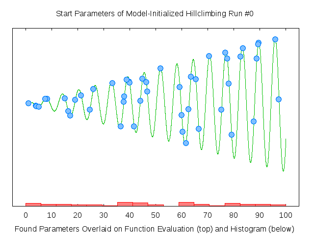
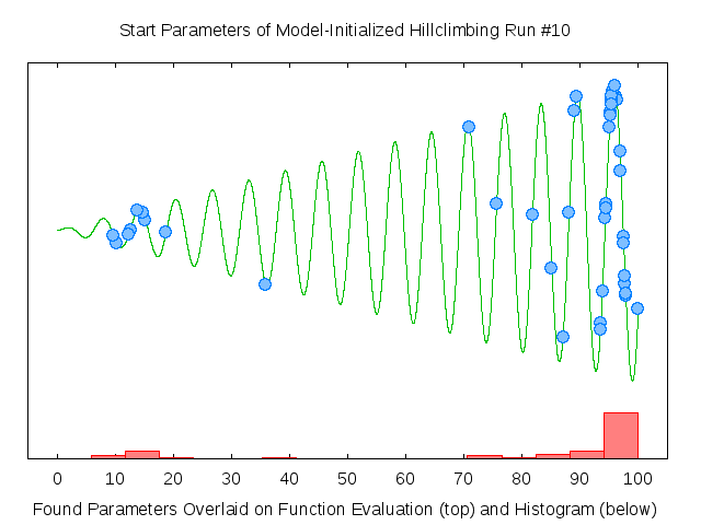
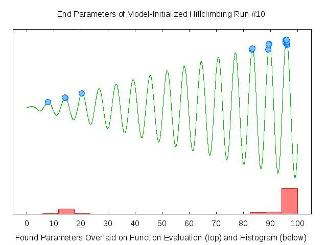
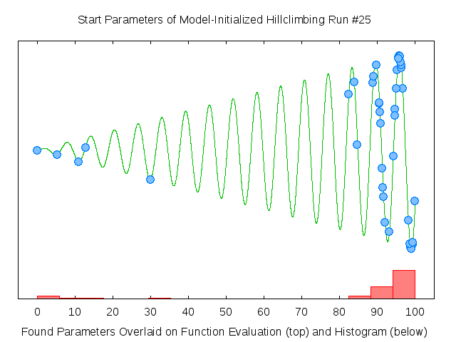
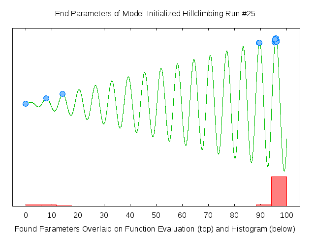
Figure 7: Sines Problem with Search-Space Modeling / Learning. Note that even at the beginning of the runs, shown in the left column of rows 2 & 3 (run #10 & #25 respectively), the hillclimbing begins in regions of high performance – thereby leading to better performance overall by the end of the hillclimbing search. In run 1 (top row, left)- since no learning has yet happened, the points are randomly distributed in the beginning of the run.

3 Empirical Results

In this section, we examine the benefits of the probabilistic model to select starting points for the NASH optimization procedure on a number of problems drawn from the literature and real-world needs. As described earlier, when the model is used, $M$ samples are generated, the best of which is used to initialize NASH. To ensure that the model is actually providing useful information and that it is not merely the process of examining $M$ samples before beginning a new run of NASH that is yielding the improved performance, three variants of NASH are explored. Though they vary in seemingly small implementation details, the effects on performance can be dramatic.

• NASH-V1: This is exactly NASH shown in Figure 3.

• NASH-V2: Before beginning the NASH run, $M$ samples are randomly generated and evaluated. The best one found from the $M$ generated is used to initialize the NASH algorithm. No learning is used here. This variant is included to test whether just the process of generating multiple samples and selecting the best prior to starting NASH is enough to provide improvement to the final result – even with no modeling.

• NASH-V3: Before beginning the NASH run, $M$ samples are generated by making small perturbations to the best solution found in all the previous NASH runs. (The first NASH run is initialized randomly). Each of the $M$ samples is then evaluated. The best sample found from the $M$ is used to initialize the NASH algorithm. This variant tests whether the neural network models actually capture the shape of the search space, or whether they are only (inefficiently) forcing search around the best solutions seen so far.

It is interesting to note that on some of the problems detailed below, adding any of these heuristics will lead to a degradation in performance. For these problems, it is likely that the search space does not contain easily learnable trends– either because large portions are flat or pocked with local-optima, or that the information cannot be correctly modeled with the networks used here. This will be discussed with the problem descriptions. Using problem-specific hand-crafted features, such as done with STAGE [25], may help.

The termination condition for each NASH run was either (1) 10,000 evaluations were performed or (2) 500 evaluations were conducted with no-improvement. The latter indicated that the search might be trapped in a local maxima. All approaches were given a total of 500,000 evaluations. The number of NASH runs that were conducted within the 500,000 evaluations was dependent on the problem and how quickly/often the algorithm was unable to escape local optima.

3.1 Noisy Evaluations

In the previous section, we used a simple Sines maximization problem as an illustrative example of how learning aids search. Due to the problem’s simplicity, most search algorithms can perform well on it. However, with the introduction of noise, a clearer separation in performance emerges.

In this version of the problem, Noisy-Sines, the evaluation was modified to include significant uniformly distributed random noise. Uniformly chosen random noise between $[0,0.5]$ was added to the evaluation. For large parts of the search space, the overall evaluation is dominated by noise (note that if the same solution is evaluated twice, the noise is chosen independently each time).

$$evaluation(\boldsymbol{x})=\dfrac{\sum_{i=1}^{50}(x_{i}*sin(x_{i}))}{50.0*100.0}+uniformNoise(0,0.5)$$ (1)

The performance of each algorithm is judged by the best solution found for the underlying objective function (as determined without the noise); no algorithm is privy to the underlying real function. The results are shown in Table 1. For each of the 5 algorithms tried (NASH-1,NASH-2,NASH-3, Deep-Opt-5-Layers, Deep-Opt-10-Layers), the best evaluation averaged over trials is listed in the first row. The last two rows show the significance of the difference between the algorithm’s performance and the performance of Deep-Opt-5-Layers and Deep-Opt-10-layers, respectively.

Table 1: Results for Noisy Sines Problem (20 Trials for Each Approach)

	NASH-1	NASH-2	NASH-3	Deep-Opt-5	Deep-Opt-10
Overall Average	0.690	0.691	0.700	0.731	0.726
Difference to Opt-5 Signif?	>99%	>99%	>99%	-	96%
Difference to Opt-10 Signif?	>99%	>99%	>99%	96%	-

3.2 Stable Marriage Reception-Party Seating

Though this problem shares part of its name with the stable marriage problem, it is more akin to knapsack/packing problems. Real versions of this problem have arisen in topics as diverse as processor scheduling to intern and group seating layouts.

In a canonical version of this problem, $G$ parties are invited to a formal-seated party, such as a wedding reception. Each party can have a variable size. Each member of the party must sit together at one of the $T$ tables, which each have a capacity $C_{t}$. The additional twist to this problem is that each $G$ has a preference with whom to sit with, expressed as a real value. The full preference matrix is $|G\times G|$. Preferences can be negative, and not constrained in magnitude. Further, it is not a requirement that each guest express a preference to every other guest, or even to any guests. Preferences may not be symmetric.

The goal is to find a seating assignment that (1) keeps the members of each group together, (2) does not seat people beyond the capacity of the table, (3) maximizes the summed happiness/preferences over all the tables. For the size of the problems explored here, the reception has 10 tables, each with capacity 12 people. Each guest’s party is randomly chosen between 1 and 3 people. Preferences were expressed as a value between [-100, +100]. The number of groups, $|G|$, was set to 50.

To encode the solution as a vector, each group was assigned T parameters, corresponding to each of T tables; there were a total of 500 $(50\times 10)$ parameters, ($realValueParameter_{g,t}$). At evaluation time, these 500 parameters were sorted from high to low. Based on the sorted list of $realValueParameter_{g,t}$ assignments were made in order from highest to smallest of group $g$ to table $t$. Note that the assignment occurred only if the group was (1) as yet unseated and (2) the table could hold the size of the group; otherwise that parameter was ignored and the next one processed. This encoding has the benefit of not only specifying each groups’ preferences to tables, but also being able to encode “how important” it is that a particular group be assigned to a particular table.

20 unique problems were created and tested with randomly generated, complete, $|G\times G|$ preference matrices. The random generation of problems led to an extremely large spread of final answers across problems. To summarize the results, we compared the five approaches, and gives the numbers of problems (out of 20) on which each algorithm obtained the highest evaluation (highest summed preferences at the tables, with all the constraints being met). The results are shown in Table 2. The next line of the table give the number of trials (out of 20) that Deep-Opt-5-layers outperformed the other 4 methods. The last line does the same for Deep-Opt-10-layers.

Table 2: Stable Marriage Reception-Party Seating: Number of times each algorithm outperformed all others (out of 20)

	NASH-1	NASH-2	NASH-3	Deep-Opt-5	Deep-Opt-10
Overall Best (Out of 20)	3	2	0	10	5
Deep-Opt-5 Outperformed(ties)	14	16	19	-	11 (1)
Deep-Opt-10 Outperformed(ties)	10	13	15	8 (1)	-

3.3 Graph Bandwidth

Given a graph with $V$ vertices and $E$ edges, the graph bandwidth problem is to label the vertices of the graph with unique integers so that the difference between the labels between any two connected vertices is minimized. Formally, as described in [36], label the $p$ vertices $v_{i}$ of a graph $G$ with distinct integers $f(v_{i})$ so that the quantity $\max\{\,|f(v_{i})-f(v_{j})|:v_{i}v_{j}\in E\,\}$ is minimized ($E$ is the edge set of $G$). More details of the complexity of this problem can be found in [37]. Interest in this problem stems from a variety of sources, including constraint satisfaction [38] and minimizing propagation delay in the layout of electronic cells.

The solution is encoded as follows: each vertex is assigned a real-valued parameter (full solution encoding of length $|V|$). The vertices are sorted according to their respective assigned values. The integers $[1..V]$ are then assigned to the vertices in their respective sort position. Once each vertex has an integer assignment, the maximum difference between the assignments of connected edges is returned. The results are shown in Table 3. This is a particularly difficult problem; ties are shown in parentheses.

Table 3: Graph Bandwidth:Number of times each algorithm outperformed all others (out of 20)

	NASH-1	NASH-2	NASH-3	Deep-Opt-5	Deep-Opt-10
Overall Best	0	0	6	10	8
Deep-Opt-5 Outperformed	20	20	12 (3)	-	6 (6)
Deep-Opt-5 Difference Signif?	>99%	>99%	96%	-	no
Deep-Opt-10 Outperformed	20	20	12 (2)	8 (6)	-
Deep-Opt-10 Difference Signif?	>99%	>99%	96%	no	-

3.4 Graph-Based Constraint Satisfaction

Constraint Satisfaction has numerous real-world applications. We recently used it for resource allocation and job scheduling. Is is presented here in its simplest form.

Simply stated, in this problem, there are $P=100$ real-value parameters in the range [0,1.0]. These parameters are assigned to the vertices in a graph. The graph contains 2,000 randomly chosen, directed, edges which specify a constraint that the origination-node must hold a value greater than the destination-node. The optimization problem is to assign values to the nodes such that as many of the 2,000 constraints are satisfied as possible. If the constraint is not met, the error is the absolute difference in the two values. The error, to be minimized, is summed over all constraints. The results are shown in Table 4.

Table 4: Real Valued Graph-Based Constraint Satisfaction: Number of times each algorithm outperformed all others (out of 20)

	NASH-1	NASH-2	NASH-3	Deep-Opt-5	Deep-Opt-10
Overall Best	0	0	2	13	5
Deep-Opt-5 Outperformed	20	20	16	-	14
Deep-Opt-5 Difference Signif?	>99%	>99%	>99%	-	no
Deep-Opt-10 Outperformed	20	20	17	6	-
Deep-Opt-10 Difference Signif?	>99%	>99%	>99%	no	-

3.5 Graph-Based Discrete Constraint Satisfaction

In this variant of the previous graph-based constraint satisfaction problem, the exact same setup is used as in Section 3.4, however, each node may only take on 1 of 16 letters – ${A..P}$. In terms of the real-world application of job scheduling mentioned above, in this version of the problem, jobs can enter the system only at specific, synchronized times. This makes the problem closer to a selection problem (where one of the 16 values is selected for each of the nodes) as compared to the previous instantiation where a real value was assigned to each node.

Though conceptually a small difference from the above encoding, discretization has enormous ramifications in the solution encoding. The simplest encoding is to use 100 real-valued outputs, one for each node, and divide the [0,1] region into 16 evenly spaced regions, each assigned to a single letter. However, for the reasons explained in Section 4.1, this encoding performs poorly. Instead, we use an encoding more amenable to selection problems and/or discrete-parameters; this encoding improves the performance of both Deep-Opt and as well as NASH alone.

The encoding used is similar to the Reception-Party-Seating task described in Section 3.2. Each vertex in the graph is assigned 16 real-valued parameters; each corresponding to a single letter ${A..P}$ (In contrast, recall that with the encoding described in Section 3.4, each vertex was simply assigned 1 real-valued parameter). In each set of 16, the maximum value is found and the corresponding letter assigned to the vertex. In sum, for a 100 node graph, 1,600 parameters are used. Once the graph nodes are assigned values, the rest of the evaluation proceeds as described in Section 3.4.

Table 5: Discrete Valued Graph-Based Constraint Satisfaction: Number of times each algorithm outperformed all others (out of 20)

	NASH-1	NASH-2	NASH-3	Deep-Opt-5	Deep-Opt-10
Overall Best	0	0	3	13	4
Deep-Opt-5 Outperformed	19	19	16	-	14
Deep-Opt-5 Difference Signif?	>99 %	>99 %	98%	-	no
Deep-Opt-10 Outperformed	19	19	14	6	-
Deep-Opt-10 Difference Signif?	>99 %	>99 %	92%	no	-

3.6 Two Dimensional Layout Problems

This section highlights the limitations of the Deep-Opt approach. A number of problems which broadly encompassed the task of two dimensional layout, did not improve significantly with search space modeling. Two of the problems are detailed here.

3.6.1 Minimizing Crossings

The goal is to find a planar layout of a graph’s nodes that minimizes edge crossings. See [39] for more details. In general, the edges can be drawn in any shape. For simplicity, in our implementation, the edges are drawn only with straight lines, this is termed the rectilinear crossing number.

For our tests, each node was represented with two parameters (x,y coordinates). Small graphs were tried with 25 nodes. This yielded a solution encoding of 50 real-values, which specified the coordinates of each point on a plane. Each graph had 50 randomly chosen connections. 20 randomly generated problem instantiations were attempted.

One of the interesting findings is that NASH-2 outperformed NASH-3. In most previous experiments, this was reversed. NASH-2 received a higher score in 12 out of the 20 problems (the scores, as measured by a standard t-test were statistically different with $p=0.96$). Recall that NASH-2 initialized each hillclimbing run by first generating a small number of random candidate solutions and selecting the best one. In contrast, NASH-3 perturbs the current best solution to determine the best starting point for NASH. Although left for future exploration, it is worth investigating what insight this gives about the search space? If searching around the current best does not yield as good results as randomly starting over, does the search space have more or less optima, or are the local optima further spread apart, deep, etc? We leave the speculation of the ramifications of NASH-2 outperforming NASH-3 to future work. However, because the Deep-Opt can just as easily be applied to NASH-2 as NASH-3, for the experiments in this section, we used it to “wrap” NASH-2. Everything else, all of the parameters, etc., remained the same.

Table 6: Results for Minimizing Crossing on 20 randomly generated problems

	NASH-1	NASH-2	NASH-3	Deep-Opt-5	Deep-Opt-10
Overall Best	1	5	3	8	3
Deep-Opt-5 Outperformed	16	11	14	-	15
Deep-Opt-5 Difference Signif?	>99%	no	97%	-	no
Deep-Opt-10 Outperformed	14	6	13	5	-
Deep-Opt-10 Difference Signif?	>97%	no	no	no	-

3.6.2 Image Approximation via Triangle Covering

This is the only problem in the paper for which the parameters for NASH were changed to be optimized for this problem. Accordingly, Deep-Opt also used the same parameters. Had these parameters not been reset, neither NASH nor Deep-Opt would perform as well as shown here, with Deep-Opt under-performing NASH alone.

In this problem, there is an intensity target image (just black and white, no color information), $I$, that is $N\times N$ pixels. The goals is to find T triangles and their intensities that approximate the image. Specifically, each triangle must specify three vertices between [0,N] in both X&Y and an intensity value. The triangles are drawn onto an initially empty canvas. The triangles may overlap; their intensities are additive. After all T triangles are drawn, the resulting image is scaled back into the appropriate space (0 .. 255 pixel intensities), and compared, pixel-wise, to the original image. The $L_{2}$ distance is to be minimized. (The problem is set up as a maximization problem by taking the the reciprocal of the summed $L_{2}$ distance.) This is a particularly difficult/interesting problem when T is small.

To set the parameters for NASH and Deep-Opt, we tested this problem with 50 triangles, trying to approximate an intensity based crop of “The Scream” by Edvard Munch. Each triangle was encoded as 7 parameters: 6 for the (x,y) coordinates of three vertices and 1 for the intensity. With 50 triangles, there were a total of ($50\times 7=$) 350 parameters in the solution encoding. Once the parameters were set, 3 other images, shown in Figure 8, were also attempted with the same parameter settings. The relative performance is given in Table 7. Note that the overall performance is virtually identical. This is averaged over 10 trials on each image.

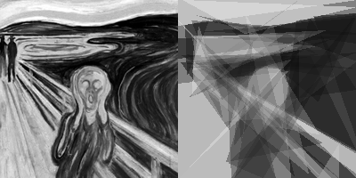
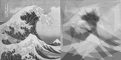
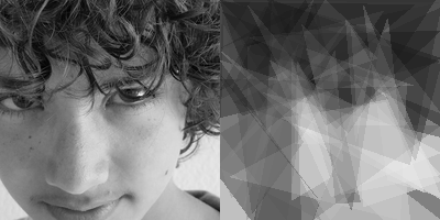
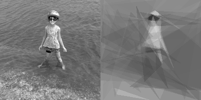
Figure 8: In each of the 4 sets of images, the left of the pair is the original image. On the right is the reconstruction of the image using the 50 triangles found by Deep-Opt.

Table 7: NASH vs. Deep-Opt on Triangle Covering - Equivalent Performance over Multiple Runs & Images

Image	Performance of NASH	Performance of Deep-Opt
The Scream	1.00	1.00
Great Wave off Kanagawa	1.00	1.001
Photograph 1	1.01	1.00
Photograph 2	1.00	1.001

4 Extensions & Alternatives

In this section, we briefly describe three extensions and further tests to the Deep-Opt. Though the results are promising, they are preliminary.

4.1 Discrete/Binary Parameters

Deep-Opt has been described with real-valued parameters. The input parameters, as well as the target output, are scaled to [0.0,1.0]. However, there are a wide variety of problems that employ discrete or binary parameters. Here, we present one method to tackle such problems.

To ground the discussion, let’s examine a simple two dimensional checkerboard problem [16]. In this problem, there is a planar $15\times 15$ grid of binary digits. The goal is to set each digit such that it is the opposite of the digits in its 4 primary directions. There are two globally optimal solutions, but there there are also many locally optimal solutions such that any single bit-flip will not yield improved performance.

First, we conducted an experiment to determine how Deep-Opt, as described to this point, would perform on this task. The solution encoding is 225 bits. In this instantiation, the maximum possible evaluation for this task is 676 (13*13*4); each of the bits in the 4 primary directions that are correctly set for the inner $13\times 13$ square contributes one point to the evaluation. The average Deep-Opt based solution quality was 537. For comparison, the three versions of NASH, without any learning, had average solution qualities of 655,655 and 668 (very close to the optimal), respectively. This difference between these and Deep-Opt is one of the largest witnessed in this entire study.

Why did this happen? In this initial attempt, the straight-forward method to interpret the real valued solution parameters as binary was used. If the real value was over 0.5, the bit was assigned to 1 and 0 otherwise. With this scheme, note that small changes to a parameter’s real value often did not yield any change in solution string (unless the value was close to 0.5) or, thereby, to its evaluation. Therefore, many solution strings appeared to have the same evaluation, though they held different values as real-valued vectors.

Ideally, if the bit position should be 1, we should favor solutions that have the real value associated with that bit position as far above 0.5 as possible (and the opposite for bit positions that should be 0). To do this, we use a technique similar to stochastic sigmoid units in training the neural network to model the search space (for a recent paper on this and related topics, see  [40]).

Recall that in the candidate generation phase (Lines 13-19 in Figure 5), we start with an input of a candidate solution vector, $s$. Over a number of iterations of back-driving the network, the inputs are modified by following the gradients needed to transform the candidate solution to one such that the network computes a value of 1.0 when the revised candidate solution is input. In the discrete version (referred to as Deep-Discrete-Opt), we instead treat each real valued parameter, $p,p\in s$ as a probability. We generate a small number of binary solutions strings (200) where each parameter in position-$p$ has a probability of being assigned a 1.0 of $p$. All of these binary solutions are then fed to the network and the gradients computed for all of the solution strings (to move the network’s evaluation of each of them closer to the target output of 1.0). Note that there is no need to evaluate each of these against the actual, real, evaluation function – only the network’s output is measured to set the error signal. Although this procedure adds to the processing time, the result are vastly improved. Out of 10 trials, 9 had perfect evaluations of 676; overall the trials had an average of 673.4. This overcomes the previous limitations of the naive implementation of binarizing the real-value parameters.

For completeness, we also tried an alternative to this procedure to determine if just increasing the learning rate in the generation process would cause enough moves across the 0.5 boundary to achieve the same benefits. A variety of larger learning rates were tried (from $2\times$ to $40\times$ the standard learning rate used previously). In no case did the performance improve. The generation of binary strings outperformed all versions with only increased learning rates.

4.2 The Role of Scaling Examples and Their Outputs

Deep-Opt, as used in this paper, works by back-driving the neural network inputs to change to cause the network to yield an output of 1.0 at its output node. Recall that the evaluations of the solutions generated in $S$ are scaled, before each training session, to values between [0.0,1.0].

Scaling the evaluations of $S$ to a fixed range leads to a subtle complexity. Note that a subset of the members of $S$ change in every training cycle: as NASH completes a hillclimbing run, some of the newly found solutions are appended to $S$ and other solutions from $S$ removed. Often, in the early parts of search, the range of the actual evaluations present in $S$ expands to include new, higher evaluation members while many of the randomly found initial members of $S$ (with low evaluations) are still present. The opposite happens in the latter parts of search; the range of values contracts as the search focuses primarily on the better solutions and all the solutions have close (high) evaluations.

Because of this, note that in trainingCycle_t, a member, $s$ may have a real evaluation of X that is scaled to X’ (when all the members of $S$ are scaled between 0 and 1.0). In trainingCycle_t+1, that same $s$, which has the same real evaluation of X, may be scaled to X”, where X” could be either greater or less than X’. Because the networks continue their training in every cycle, this has not proven to be a problem as the change in evaluation seems to be quickly recovered; this may be because the relative ordering of the samples does not change. However, in the future, it will be interesting to try variants in which the re-scaling is not done. This may require engineering the setup of the problems so that they always output values in a fixed, a priori known, range.

This expansion and contraction dynamic process happens implicitly through the addition of new members of $S$ as search progresses. Returning to the Sine problem, we can witness the convergence of the minimum and maximum values represented in $S$ as new items are added to $S$ (shown with a small $|S|$ =5000); see Figure 9. The important trend is that the minimum and maximum values rapidly converge. This does not necessarily imply that all the candidate solutions in $|S|$ are similar (though likely many are); it does mean that they are close in performance . The rate of this convergence corresponds to the exploitation vs. exploration trade-off.

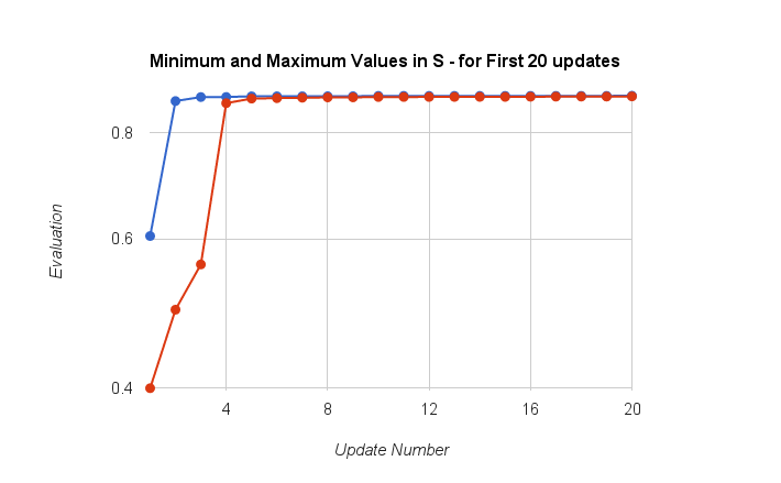
Figure 9: Notice the rapidly diminished difference in evaluations between the best and worst members of $S$ as search progresses. $S$ is the set of candidate solutions from which the probabilistic model is created.

One can imagine that instead of scaling the target outputs to values in the range [0.0,1.0], they were scaled to [0.0,$Z$], where $Z<1.0$. In this approach, the highest scoring $s\in S$ will have a value of $Z$. When the network is back-driven, it is still driven to find solutions that produce a 1.0 in the output. Semantically, this attempts to create new solutions that are explicitly better than, not just equal to, those seen so far. The success of this approach is pinned on the network’s successful extrapolation of the underlying search surface to regions of better performance. Many versions of this were tried, where $Z$ was set to [0.2,0.5,0.8,0.9,0.95, and 0.99] in various experiments. Although the results are preliminary, setting the $Z$ to 0.95 and higher had little effect on the results, when compared to setting $Z=1.0$. Setting $Z$ in the low range often hurt performance. Further exploration is left for future work.

4.3 Alternative Underlying Search Algorithms

In this paper, we have coupled the use of deep-net modeling with an extremely simple, fast, localized search algorithm, NASH. It is important to also consider the possibility of using alternate search algorithms with the same modeling procedures. It is obvious how alternative search heuristics such as simulated annealing [41] and TABU search [42] can easily be substituted as they are often used to search neighborhoods around a single point in a manner similar to NASH. Although we will not delve into the general debate of the merits of these simple techniques with more sophisticated search techniques, as this has been an active area of discussion for several decades  [31] [43] [32] [33] [44] [45] [46], it is interesting, to consider the use of the probabilistic models with very different search paradigms, such as genetic algorithms.

Recall that, unlike NASH, genetic algorithms work from a population of points. Members of the population are created with recombination operators (crossover) that combine the elements of two or more candidate solutions. The newly created solutions are further randomly perturbed (mutated) to reveal the ’children’ solutions that are the candidate solutions to evaluate next [5]. Numerous variations of GAs and task-specific operators are possible and have been explored in the research literature. Next, we perform a set of tests using a a simple-GA with the parameters shown in Table 8. These are typical of GAs used for static optimization problems in the literature. To learn more about GAs, please see [5].

Table 8: GA Parameters

Parameter	Value
Population-Size	50 (trial #1), 100 (trial #2)
Crossover-Type	Uniform
Mutation-Rate	2%
Steady-state vs. generational	Generational
Number of Evaluations before restart	10,000
Elitist Selection	Yes - Single best member always survives from $generation_{t}$ to $generation_{t+1}$

We test the GA with two population sizes (50 & 100) run for an equivalent number of function evaluations as all of the previous runs with hillclimbing (500,000). Additionally, as with the previous runs, the GA was restarted after 10,000 evaluations. In the standard GA, the initial population is comprised of candidate solutions that were randomly generated. In the Deep-Opt-GA, the initial population of candidate solutions is entirely generated from the back-driven neural network model.

This approach was tested on the same real-valued constraints problems described in Section 3.4. The results are shown in Table 9. Deep-Opt-GA outperformed the random initialization on all 20 instantiations attempted, for both sets of trials (with population size 50 and 100). The population size did not make a significant difference. Although not directly relevant to the effects of Deep-Opt, it is interesting to note how these results compare to the hillclimbing runs described in Section 3.4. Even the simplest NASH (NASH-1), with a performance of 5206, did better than the GA models tested; though the GA models were consistently improved with learning. To summarize the findings in this section, using models to guide search can help even in search heuristics that operate from more than a single point – those that are population-based, such as genetic algorithms.

Table 9: GA performance on Graph-Based Constraints Problem (20 Instantiations)

Approach	Performance	Number of Wins
Standard GA (population size 50)	4817	0
Deep-Opt-GA (population size 50)	5120	20
Standard GA (population size 100)	4825	0
Deep-Opt-GA (population size 100)	5131	20

5 Discussion and Future Work

We have presented a novel method to incorporate deep-learning with stochastic optimization. It is the next instantiation of intelligent model-based stochastic optimization and follows in the tradition of the probabilistic model based optimization approaches from the last two decades of research. An important aspect of this work is that a priori information about the problem is minimal in setting the form of the model. In this study, two multi-layer feed-forward networks with 5 and 10 hidden layers were used on all of the problems with no problem-specific modifications. With the judicious use of early-stopping in training, the potential downsides for overtraining were overcome.

A consideration that we did not discuss in this paper is the speed of optimization. Between every hillclimbing run, a network is trained and sampled; this can be a time consuming procedure on the problems with the large solution-encoding (e.g. the discrete constraint satisfaction problem). As yet, we have not made attempts to optimize this; however, in the future, methods that employ fewer training steps between hillclimbing runs should be explored. It is likely that will achieve similarly positive results.

Many of the advances from the rapidly evolving field of deep learning can be directly incorporated into this work (such as network shrinking, rapid training, regularization schemes, etc.), as continuously training networks is the core of the learning system. Outside of the deep-learning advancements, three avenues of immediate interest for future explorations are given below.

First, the overarching goal of this paper was to concretely demonstrate the integration of neural network learning with optimization, not to promote this system as finalized optimization system. To make a finalized optimization system, further exploration of the algorithm’s robustness and behavior is warranted. For example, there are many parameters in this system. In this study, we have found that the results are most sensitive to the size of $|S|$ and to the decision of when to restart training the network from scratch – this happens when new samples are added to $|S|$ and the network fails to accommodate them in learning (i.e. the error on the samples does not reduce). This may be because of the scaling issues mentioned in Section 4.2 and/or because the weights of the network may have grown too large. The beneficial effects of regularization may be especially pronounced in this application as networks are constantly being incrementally trained with changing data. Also, we have found a class of problems for which we have not observed a benefit of using the modeling (see Section 3.6). Are the problems too easy or too hard, or is an alternate representation needed?

Second, an alternative to using the network back-driving technique to generate candidate initialization points is to simply use the network as a proxy evaluation function for hillclimbing. In this approach, hillclimbing (NASH) is conducted directly on the model’s output. After every perturbation, the new candidate-solution is passed through the network to measure it’s estimated performance. This, unlike network back-driving, does not take advantage of the fact that the network is differentiable, and rather only uses it as a proxy for the real evaluation function. However, it may reveal parts of the search space that back-driving may not.

The third, and perhaps the most speculative, direction is to measure if there are transferable features that are learned between different instantiations of the same problem. For example, with respect to the triangle-covering problem presented in Section 3.6.2, once we have learned how to evaluate how well a set of triangles reproduces an image, is learning the evaluations for the next image easier? One can imagine that low level primitives of how to draw triangles, if they are indeed learned by the network, may be reusable. Even if there is little transference in the current implementation, exploring problem transference has enormous potential to make this system automatically more intelligent with time.

Acknowledgments

The author would like to gratefully acknowledge Sergey Ioffe and Rif A. Saurous for their invaluable comments.

References

- [1] S. Baluja, “Population-based incremental learning. a method for integrating genetic search based function optimization and competitive learning,” CMU-CS-94-163. Carnegie Mellon University, Dept. of Computer Science, Tech. Rep., 1994.
- [2] A. Juels, Topics in black-box combinatorial optimization. University of California, Berkeley, 1996.
- [3] H. Mühlenbein and G. Paass, “From recombination of genes to the estimation of distributions i. binary parameters,” in International Conference on Parallel Problem Solving from Nature. Springer, 1996, pp. 178–187.
- [4] G. R. Harik, F. G. Lobo, and D. E. Goldberg, “The compact genetic algorithm,” IEEE transactions on evolutionary computation, vol. 3, no. 4, pp. 287–297, 1999.
- [5] D. E. Goldberg, Genetic algorithms in search, optimization, and machine learning. Addison-Wesley Publishing Company, 1989.
- [6] J. H. Holland, Adaptation in natural and artificial systems: an introductory analysis with applications to biology, control, and artificial intelligence. U Michigan Press, 1975.
- [7] K. De Jong, “Genetic algorithms: a 30 year perspective,” Perspectives on Adaptation in Natural and Artificial Systems, vol. 11, 2005.
- [8] G. Syswerda, “Simulated crossover in genetic algorithms,” Foundations of Genetic Algorithms, vol. 2, pp. 239–255, 1993.
- [9] M. A. Thathachar and P. S. Sastry, “Learning optimal discriminant functions through a cooperative game of automata,” IEEE Transactions on Systems, Man, and Cybernetics, vol. 17, no. 1, pp. 73–85, 1987.
- [10] V. Kvasnicka, M. Pelikán, and J. Pospichal, “Hill climbing with learning (an abstraction of genetic algorithm),” in Neural Network World, 6. Citeseer, 1995.
- [11] M. Hohfeld and G. Rudolph, “Towards a theory of population based incremental learning,” in Proceedings of the International Conference on Evolutionary Computation, 1997.
- [12] R. Rastegar, A. Hariri, and M. Mazoochi, “A convergence proof for the population based incremental learning algorithm,” in 17th IEEE International Conference on Tools with Artificial Intelligence (ICTAI’05). IEEE, 2005, pp. 387–391.
- [13] C. Gonzalez, J. A. Lozano, and P. Larrañaga, “The convergence behavior of the pbil algorithm: a preliminary approach,” in Artificial Neural Nets and Genetic Algorithms. Springer, 2001, pp. 228–231.
- [14] C. González, J. A. Lozano, and P. Larranaga, “Analyzing the population based incremental learning algorithm by means of discrete dynamical systems,” Complex Systems, vol. 12, pp. 465–479, 2000.
- [15] J. S. De Bonet, C. L. Isbell, P. Viola et al., “Mimic: Finding optima by estimating probability densities,” Advances in neural information processing systems, pp. 424–430, 1997.
- [16] S. Baluja and S. Davies, “Fast probabilistic modeling for combinatorial optimization,” in AAAI/IAAI. Madison, WI, USA, 1998, pp. 469–476.
- [17] C. Chow and C. Liu, “Approximating discrete probability distributions with dependence trees,” IEEE transactions on Information Theory, vol. 14, no. 3, pp. 462–467, 1968.
- [18] S. Baluja and S. Davies, “Using optimal dependency-trees for combinatorial optimization,” in International Conference on Machine Learning (ICML), 1997, pp. 30–38.
- [19] D. Heckerman, “A tutorial on learning with bayesian networks,” in Innovations in Bayesian networks. Springer, 2008, pp. 33–82.
- [20] J. Pearl and S. Russell, “Bayesian networks,” Department of Statistics, UCLA, 2000.
- [21] M. Pelikan, D. E. Goldberg, and E. Cantú-Paz, “Boa: The bayesian optimization algorithm,” in Proceedings of the 1st Annual Conference on Genetic and Evolutionary Computation-Volume 1. Morgan Kaufmann Publishers Inc., 1999, pp. 525–532.
- [22] J. Yao, Y. Kong, and L. Yang, “Bayesian optimization algorithm based on incremental model building,” in International Symposium on Intelligence Computation and Applications. Springer, 2015, pp. 202–209.
- [23] R. Etxeberria and P. Larranaga, “Global optimization using bayesian networks,” in Second Symposium on Artificial Intelligence (CIMAF-99). Habana, Cuba, 1999, pp. 332–339.
- [24] M. Pelikan, K. Sastry, and E. Cantú-Paz, Scalable optimization via probabilistic modeling: From algorithms to applications. Springer, 2007, vol. 33.
- [25] J. Boyan and A. W. Moore, “Learning evaluation functions to improve optimization by local search,” Journal of Machine Learning Research, vol. 1, no. Nov, pp. 77–112, 2000.
- [26] K. Hornik, M. Stinchcombe, and H. White, “Multilayer feedforward networks are universal approximators,” Neural networks, vol. 2, no. 5, pp. 359–366, 1989.
- [27] A. Linden and J. Kindermann, “Inversion of multilayer nets,” in Neural Networks, 1989. IJCNN., International Joint Conference on. IEEE, 1989, pp. 425–430.
- [28] L. Gatys, A. S. Ecker, and M. Bethge, “Texture synthesis using convolutional neural networks,” in Advances in Neural Information Processing Systems, 2015, pp. 262–270.
- [29] L. A. Gatys, A. S. Ecker, and M. Bethge, “A neural algorithm of artistic style,” arXiv preprint arXiv:1508.06576, 2015.
- [30] D. P. Kingma and J. Ba, “Adam: A method for stochastic optimization,” CoRR, vol. abs/1412.6980, 2014. [Online]. Available: http://arxiv.org/abs/1412.6980
- [31] A. Juels and M. Wattenberg, “Stochastic hillclimbing as a baseline method for evaluating genetic algorithms,” in Proceedings of the 1995 Conference on Neural Information Processing Systems (NIPS), vol. 8, 1996, p. 430.
- [32] S. Baluja, “An empirical comparison of seven iterative and evolutionary function optimzation heuristics,” Computer Science Department, Tech. Rep. CMU-CS-95-193, September 1995.
- [33] M. Mitchell, J. H. Holland, and S. Forrest, “When will a genetic algorithm outperform hill climbing,” in Advances in Neural Information Processing Systems 6, J. D. Cowan, G. Tesauro, and J. Alspector, Eds. Morgan-Kaufmann, 1994, pp. 51–58. [Online]. Available: http://papers.nips.cc/paper/836-when-will-a-genetic-algorithm-outperform-hill-climbing.pdf
- [34] M. Covell, S. Baluja, and R. Sukthankar, “Micro-auction based traffic light control: Responsive, local decision making,” in IEEE Intelligent Transportation Systems Conference-2015, 2015.
- [35] Chriddyp. (2017) Asyncho from 0.00 to 0.05. [Online]. Available: https://plot.ly/~chriddyp/
- [36] Wikipedia. (2016) Graph bandwidth. [Online]. Available: https://en.wikipedia.org/wiki/Graph_bandwidth
- [37] P. Z. Chinn, J. Chvátalová, A. K. Dewdney, and N. E. Gibbs, “The bandwidth problem for graphs and matrices—a survey,” Journal of Graph Theory, vol. 6, no. 3, pp. 223–254, 1982.
- [38] R. Zabih, “Some applications of graph bandwidth to constraint satisfaction problems.” in AAAI, 1990, pp. 46–51.
- [39] Wikipedia. (2016) Crossing number (graph theory). [Online]. Available: https://en.wikipedia.org/wiki/Crossing_number_%28graph_theory%29
- [40] T. Raiko, M. Berglund, G. Alain, and L. Dinh, “Techniques for learning binary stochastic feedforward neural networks,” arXiv preprint arXiv:1406.2989, 2014.
- [41] S. Kirkpatrick, C. D. Gelatt, M. P. Vecchi et al., “Optimization by simulated annealing,” Science, vol. 220, no. 4598, pp. 671–680, 1983.
- [42] F. Glover, “Tabu search-part i,” ORSA Journal on computing, vol. 1, no. 3, pp. 190–206, 1989.
- [43] K. J. Lang, “Hill climbing beats genetic search on a boolean circuit synthesis problem of koza’s,” in Proceedings of the Twelfth International Conference on Machine Learning, 1995, pp. 340–343.
- [44] P. Ross and D. Corne, “Comparing genetic algorithms, simulated annealing, and stochastic hillclimbing on timetabling problems,” in AISB Workshop on Evolutionary Computing. Springer, 1995, pp. 94–102.
- [45] F. G. Lobo and M. Bazargani, “When hillclimbers beat genetic algorithms in multimodal optimization,” in Proceedings of the Companion Publication of the 2015 Annual Conference on Genetic and Evolutionary Computation. ACM, 2015, pp. 1421–1422.
- [46] K. A. De Jong, “Genetic algorithms are not function optimizers,” Foundations of genetic algorithms, vol. 2, pp. 5–17, 1993.