Change in the Orbital Period of a Binary System Due to Dynamical Tides for Main-Sequence Stars

Abstract

We investigate the change in the orbital period of a binary system due to dynamical tides by taking into account the evolution of a main-sequence star. Three stars with masses of one, one and a half, and two solar masses are considered. A star of one solar mass at lifetimes $t=4.57\times 10^{9}$ yr closely corresponds to our Sun. We show that a planet of one Jupiter mass revolving around a star of one solar mass will fall onto the star in the main-sequence lifetime of the star due to dynamical tides if the initial orbital period of the planet is less than $P_{\rm orb}\approx 2.8$ days. Planets of one Jupiter mass with an orbital period$P_{\rm orb}\approx 2$ days or shorter will fall onto a star of one and a half and two solar masses in the mainsequence lifetime of the star.

I Introduction

Tidal interactions play an important role in dynamical processes in the two-body problem in close binary systems: star–star (binary star) or star– planet. They can lead to such phenomena as synchronization and orbital circularization (Hut 1981; Zahn 1977) as well as to the tidal capture (Press and Teukolsky 1977) or disruption of an object (star) (Ivanov and Novikov 2001) and the fall of the object onto the star (Rasio et al. 1996; Penev et al. 2012; Bolmont and Mathis 2016). In this paper we consider the tidal interaction of two bodies: a star and a point source. The point source can be both a star (a neutron star, a white dwarf, etc.) and a planet. Below we will call the point source a planet by implying that this can also be a star. Since the evolution time scales of the eccentricity or semimajor axis strongly depend on the orbital period of the binary system and for some stellar models can take values up to 108 yr or more for periods of about 5 days (Ivanov et al. 2013; Chernov et al. 2013), the evolution of the star itself should be taken into account on such time scales. As the star evolves, the orbital parameters change due to tidal interactions. In this paper we investigate the dynamical tides by taking into account the stellar evolution. For our study we chose three types of stars with masses of one, one and a half, and two solar masses. We consider all stars without allowance for their rotation and magnetic field and touch on the stellar physics itself superficially, as far as this problem requires. The star of one solar mass at lifetimes $t=4.57\times 10^{9}$ yr closely corresponds to our Sun and has a radiative core and a convective envelope on the main sequence. The other two stars of one and a half and two solar masses are more massive and have a more complex structure. These stars have a convective core and a radiative envelope on the main sequence (a more precise structure is presented below).

The problem of determining the tidal evolution is reduced to the problem of determining the normal modes of stellar perturbations and to calculating the energy and angular momentum exchange in the star.planet system (Ivanov and Papaloizou 2004, 2010; Papaloizou and Ivanov 2010; Lanza and Mathis 2016). The low-frequency g-modes of the stellar oscillations play an important role in the theory of dynamical tides. The tidal interactions are fairly intense at small periastron distances of the planet. For a periastron distance $a\approx 0.01$ AU, the dimensionless excitation frequency is $\tilde{\omega}\sim 0.3$, which corresponds to g-modes.

A large number of exoplanets in stellar systems have been discovered in the last few years owing to the Kepler, SuperWasp, and other observational programs. In particular, short-period massive planets with an orbital period of a few days, the so-called hot Jupiters, have been detected (Winn 2015). As a rule, the hot Jupiters have low eccentricities, which points to the importance of tidal interactions (Ogilvie 2014). The results of this paper can be directly applied to some of such systems. For example, the system YBP1194 is a solar twin (Brucalassi et al. 2014). A planet with a mass of 0.34$M_{J}$ and a period of only 6.9 days revolves around this star. For such a short-period planet the dynamical tides must be fairly intense and must affect the orbital evolution. Predictions about the subsequent evolution of this planet can be made by analyzing this system.

One of the results of this evolution is the fall of the planet onto the star. The possibility of such a fall has been considered in many papers (see, e.g., Rasio et al. 1996; Penev et al. 2012; Weinberg et al. 2012; Essick and Weinberg 2016). Rasio et al. (1996) considered the possibility of the fall of the planet onto the star due to quasi-static tides and provided a plot for solar-like stars that shows the threshold, as a function of planetary mass and orbital period, below which the planet falls onto the star. Penev et al. (2012) considered tides with a constant tidal quality factor $Q^{{}^{\prime}}$ specified phenomenologically. In reality, this factor will depend on the planet’s orbital period (Ivanov et al. 2013) and stellar age. Essick and Weinberg (2016) took into account the energy dissipation due to nonlinear interaction of modes with one another. In contrast to our approach (Ivanov et al. 2013; Chernov et al. (2013), the simultaneous solution of a large number of ordinary differential equations for each stellar model is suggested, with only solar-type stars having been considered.

In this paper we consider the evolution of stars with masses of one, one and a half, and two solar masses. Data on the stars are presented in Tables 1– 3. A novelty of this study is a consistent allowance for the stellar evolution. For each moment of the star’s lifetime we calculated the spectra of normal modes, the overlap integrals (Press and Teukolsky 1977), which are a measure of the intensity of tidal interactions (for a generalization to the case of a rotating star, see Papaloizou and Ivanov 2005; Ivanov and Papaloizou 2007), and the time scales of the orbital parameters (the tidal quality factor $Q^{{}^{\prime}}$). The overlap integrals are directly related to the tidal resonance coefficients that were introduced by Cowling (1941) (see also Rocca 1987; Zahn 1970).

All of the quantities marked by a tilde are dimensionless; the normalization is presented in Appendix A.

II FORMULATION OF THE PROBLEM

Such a quantity as the overlap integral Q is of great importance in the theory of dynamical tides. It is specified by the expression (Press and Teukolsky 1977; Zahn 1970)

$$\tilde{Q} = \sqrt{\frac{3}{4\pi}}\frac{\int\limits_{0}^{1}x^{l+1}\tilde{\rho}l(\xi_{r}+(l+1)\xi_{s})dx}{\sqrt{\int\limits_{0}^{1}x^{2}\tilde{\rho}(\xi_{r}^{2}+l(l+1)\xi_{s}^{2})dx}},$$

$$Q = \tilde{Q}\sqrt{M}R,$$ (1)

where M is the stellar mass, R is the stellar radius, and $\tilde{Q}$ is the dimensionless overlap integral; the remaining quantities and their dimensionless forms are defined in Appendix A. The overlap integral serves as a measure of the intensity of the tidal forces and plays a crucial role in the physics of dynamical tides (Press and Teukolsky 1977; Zahn 1970, 1975, 1977). Here, we will consider only the quadrupole part of the tidal forces $l=2$, because it is this part that makes the greatest contribution to the overlap integral (Press and Teukolsky 1977). The change in orbital semimajor axis and eccentricity with time is determined from the energy and angularmomentum conservation laws and is specified by the following formulas (Ivanov et al. 2013):

$$\frac{\dot{a}}{a}=-\frac{2}{T_{a}},\qquad\frac{\dot{e}}{e}=-\frac{1}{T_{e}},$$ (2)

Here, $e$ is the orbital eccentricity, $a$ is the semimajor axis, and the time scales of the change in semimajor axis $T_{a}$ and eccentricity $T_{e}$ in the case of low eccentricities ($e\rightarrow 0$) are specified by the relations (Ivanov et al. 2013)

$$T_{a}=-\frac{GMM_{2}}{a\dot{E}_{I}},\quad T_{e}=-\frac{GMM_{2}e^{2}}{a\dot{E}_{e}},$$ (3)

where $M_{2}$ is the planetary mass. The rate of change of energy $\dot{E}_{I}$, $\dot{E}_{e}$ in the case of a dense spectrum and moderately large viscosities is specified by Eqs. (51) from Ivanov et al. (2013). The spectrum is deemed to be dense enough if $\frac{d\tilde{\omega}}{dj}<<\tilde{\omega}$. For simplicity, we will consider here only the time scales of the changes in semimajor axis. Using formulas from Subsection 7.1 of the paper by Ivanov et al. (2013), we obtain

$$T_{a}=\frac{10}{3\pi^{2}}\bigg{|}\frac{d\tilde{\omega}}{dj}\bigg{|}\frac{(1+\mu)^{5/3}}{\mu\tilde{Q}^{2}\Omega_{\ast}}\left(\frac{P_{\rm orb}\Omega_{\ast}}{2\pi}\right)^{10/3},$$ (4)

where $\mu=\frac{M_{2}}{M}$ is the ratio of the planetary mass to the stellar mass, $\frac{d\tilde{\omega}}{dj}$ is the difference between adjacent frequencies, $j$ is the frequency number, and $\Omega_{\ast}=\sqrt{\frac{GM}{R^{3}}}$ (Ivanov et al. 2013). The orbital period of the planet around the star is specified by the relation

$$P_{\rm orb}=2\pi\sqrt{\frac{a^{3}}{G(M+M_{2})}}.$$ (5)

Below, using Eqs. (4) and (5) and solving Eq. (2), we will present the change in the planet’s orbital period as a function of time by taking into account the stellar evolution.

As is clear from Eq. (1), the eigenfunctions and, accordingly, eigenfrequencies of the stellar oscillations should be known to calculate the overlap integral. There exist three types of eigenfrequencies for a nonrotating star: the so-called p-, f-, and g-modes. We will be concerned only with the low-frequency g- modes. The properties of the g-modes are determined by the Brunt - V$\ddot{\rm a}$is$\ddot{\rm a}$l$\ddot{\rm a}$ frequency. It is specified as follows (Christensen-Dalsgaard 1998):

$$N^{2}=g\left(\frac{1}{\Gamma p}\frac{\partial p}{\partial r}-\frac{1}{\rho}\frac{\partial\rho}{\partial r}\right),$$ (6)

where $p$ is the pressure, $\rho$ is the density, $g$ is the gravitational acceleration, $\Gamma=(\partial\ln p/\partial\ln\rho)_{\rm ad}$ is the adiabatic index. However, this definition of the Brunt - V$\ddot{\rm a}$is$\ddot{\rm a}$l$\ddot{\rm a}$ frequency is difficult to apply to many stars. This is related to the numerical errors, to the calculation of the derivative of the density, and to the fact that there exist regions in stars where both terms in parentheses can be of the same order of magnitude. Therefore, a different definition is used (Brassard et al. 1991):

$$N^{2}=\frac{g^{2}\rho}{P}\frac{\chi_{T}}{\chi_{\rho}}\bigg{[}\nabla_{\rm ad}-\nabla-\frac{1}{\chi_{T}}\sum_{i=1}^{N-1}\chi_{X_{i}}\frac{d\ln X_{i}}{d\ln p}\bigg{]},$$ (7)

where

$$\nabla_{\rm ad}=\left(\frac{\partial\ln T}{\partial\ln P}\right)_{{\rm ad},X_{i}},\quad\chi_{T}=\left(\frac{\partial\ln p}{\partial\ln T}\right)_{\rho,X_{i}},$$

$$\chi_{\rho}=\left(\frac{\partial\ln p}{\partial\ln\rho}\right)_{T,X_{i}},\quad\chi_{X_{i}}=\left(\frac{\partial\ln p}{\partial\ln X_{i}}\right)_{\rho,T,X_{i\neq j}},$$ (8)

the temperature gradient

$$\nabla=\frac{\partial\ln T}{\partial\ln P},$$ (9)

$X_{i}$ is the mass fraction of atoms of type i, and

$$\sum_{i=1}^{N-1}X_{i}+X_{N}=1.$$ (10)

It is convenient to divide the Brunt - V$\ddot{\rm a}$is$\ddot{\rm a}$l$\ddot{\rm a}$ frequency into two parts: the structural part (structure terms) Brunt - V$\ddot{\rm a}$is$\ddot{\rm a}$l$\ddot{\rm a}$

$$N^{2}_{\rm st}=\frac{g^{2}\rho}{P}\frac{\chi_{T}}{\chi_{\rho}}\bigg{[}\nabla_{\rm ad}-\nabla\bigg{]}$$ (11)

and the compositional part

$$N^{2}_{\rm com}=-\frac{g^{2}\rho}{P}\frac{1}{\chi_{\rho}}\sum_{i=1}^{N-1}\chi_{X_{i}}\frac{d\ln X_{i}}{d\ln p}.$$ (12)

The compositional part is related to the change in stellar chemical composition due to nuclear reactions, and it is of great importance at the boundary of the convective and radiative regions. Another important stellar characteristic is the acoustic frequency defined by the formula

$$S^{2}_{l}=\frac{l(l+1)c^{2}}{r^{2}}.$$ (13)

The low-frequency g-modes are excited at $\omega^{2}<N^{2}$. The high-frequency p-modes are excited at $\omega^{2}>S^{2}_{l}$. We will not consider the p-modes, because they play a secondary role in the theory of dynamical tides.

Thus, the problem is reduced to finding the eigenfunctions and eigenfrequencies of the stellar oscillations, calculating the overlap integrals, and calculating the characteristic orbital parameters as a function of time. The equations that describe the eigenfrequencies and eigenfunctions of a star in the adiabatic and Cowling approximations are presented in Appendix A. The stars were modeled with the MESA software package (Paxton et al. 2011, 2013, 2015); the data obtained were then interpolated by the Steffen (1990) method to two million points. Using these data, we solved the eigenfrequency and eigenfunction problem and calculated the overlap integrals. The fourth-order Runge–Kutta method was used to solve the differential equations. The data for the stars and the overlap integrals were compared with those from Ivanov et al. (2013) and Chernov et al. (2013).

III RESULTS

In this section we present the results of our calculations of the change in the planet’s orbital period for three types of stars with masses of one, one and a half, and two solar masses. The course of stellar evolution for these models is shown on the Hertzsprung– Russell diagram depicted in Fig. 1. Data for each star are presented in the tables in Appendix B. The main phase of stellar evolution is the main-sequence phase. It is at this phase that any star spends most of its lifetime. This phase is indicated in Fig. 1 by the nearly horizontal straight line.

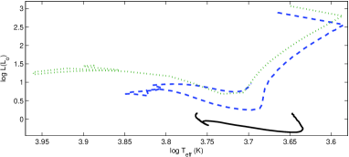
Figure 1: Hertzsprung–Russell diagram for three stars: the solid, dashed, and dotted lines are for the Sun, the star of one and a half solar masses, and the star of two solar masses, respectively.

III.1 The Sun

In this section we present the results of our calculations of the overlap integrals for various lifetimes of the star of one solar mass and the change in the planet’s orbital period with time. The star was modeled from $t=1.46\times 10^{6}$ to $t=8.61\times 10^{9}$ yr. At times $t=4.57\times 10^{9}$ yr this star closely corresponds to our Sun, and below we will call this star the Sun. At the initial time the Sun was completely convective, hydrogen burning has not yet begun, and its metallicity is z = 0.02. Figure 2 shows a dimensionless dependence of the solar density on radius at the initial and subsequent times.

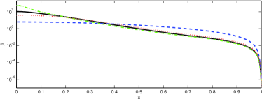
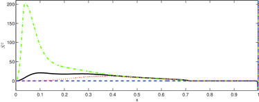
Figure 2: Density (a) and Brunt - V$\ddot{\rm a}$is$\ddot{\rm a}$l$\ddot{\rm a}$ frequency (b) for the Sun versus radius for various times: the dashed, dotted, solid, and dash–dotted lines are for the ages $t=1.46\times 10^{6}$, $t=1.02\times 10^{8}$, $t=4.57\times 10^{9}$, and $t=8.61\times 10^{9}$ yr, respectively.

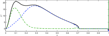
Figure 3: Brunt - V$\ddot{\rm a}$is$\ddot{\rm a}$l$\ddot{\rm a}$ frequency versus radius for the solar age $t=4.57\times 10^{9}$: the solid, dashed, and dash-dotted lines indicate the total Brunt - V$\ddot{\rm a}$is$\ddot{\rm a}$l$\ddot{\rm a}$ frequency $N^{2}$, the structural part $N^{2}_{\rm st}$, and the compositional part $N^{2}_{\rm com}$, respectively.

The course of stellar evolution and the excitation of eigenmodes can be described as follows. At times $t\approx 1.46\times 10^{6}$ yr the Sun was completely convective ($N^{2}<0$) and, therefore, no low-frequency g-modes were excited, but only the high-frequency f- and p-modes were excited. Subsequently, as the Sun evolves (at times $t\approx 1.5\times 10^{6}$ yr) a radiative region (radiative core) where the Brunt - V$\ddot{\rm a}$is$\ddot{\rm a}$l$\ddot{\rm a}$ frequency is greater than zero ($N^{2}>0$) appears and, consequently, the excitation of low-frequency g-modes begins. Only the structural part makes a major contribution to the Brunt - V$\ddot{\rm a}$is$\ddot{\rm a}$l$\ddot{\rm a}$ frequency; the compositional part is zero. This is because at such lifetimes of the Sun hydrogen burning makes a minor contribution to the energetics and evolution dynamics of the Sun. In the course of subsequent evolution the radiative region expands, the number of lowfrequency g-modes increases, and their spectrum becomes dense. The low-frequency g-modes begin to play an increasingly important role. At times $t\approx 2\times 10^{7}$ yr hydrogen burning begins to make an increasingly large contribution to the total energy of the star and, consequently, the compositional part of the Brunt - V$\ddot{\rm a}$is$\ddot{\rm a}$l$\ddot{\rm a}$ frequency also begins to contribute to the total frequency. In the course of subsequent evolution, as hydrogen burns, this contribution becomes progressively larger. One of the problems being investigated here is to take into account the evolution of the Brunt - V$\ddot{\rm a}$is$\ddot{\rm a}$l$\ddot{\rm a}$ frequency and the influence of this evolution on the tidal interactions. The radiative region expands approximately to a radius $r\approx 0.73R_{\odot}$. For the present Sun the boundary between the radiative and convective regions is $r\approx 0.712R_{\odot}$. In Fig. 2 the Brunt - V$\ddot{\rm a}$is$\ddot{\rm a}$l$\ddot{\rm a}$ frequency is plotted against radius for various stellar evolution times. It can be seen from the plot that the Brunt - V$\ddot{\rm a}$is$\ddot{\rm a}$l$\ddot{\rm a}$ frequency is subject to significant changes as the solar age increases; both the frequency spectrum and its density change accordingly, which can directly affect the tidal forces. In Fig. 3 the Brunt - V$\ddot{\rm a}$is$\ddot{\rm a}$l$\ddot{\rm a}$ frequency is plotted against radius for the present Sun. It follows from this plot that the Brunt - V$\ddot{\rm a}$is$\ddot{\rm a}$l$\ddot{\rm a}$ frequency exhibits a double-humped structure. The first and second humps are associated with the compositional and structural parts of the Brunt - V$\ddot{\rm a}$is$\ddot{\rm a}$l$\ddot{\rm a}$ frequency, respectively. At a solar age $t\approx 8.61\times 10^{9}$ yr the two contributions become comparable.

The overlap integrals (1) are plotted against frequency in the Cowling approximation in Fig. 4. For a solar age $t\approx 1.46\times 10^{6}$ yr, as has been said above, only the f- and p-modes exist; therefore, there is no low-frequency part of the spectrum. It can be seen from the plot that the absolute value of the overlap integrals decreases in the low-frequency part of the spectrum as the Sun evolves. This decrease is gradual, because the stellar structure does not change in the evolution time of the Sun. On the main sequence the Sun always has a radiative core and a convective envelope. In the high-frequency part of the spectrum, as the stellar age increases, the absolute value of the overlap integrals increases and a characteristic structure appears in the spectrumin the form of kinks.

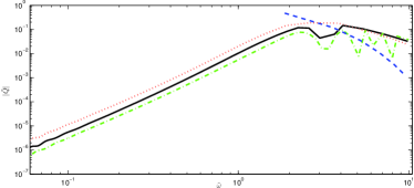
Figure 4: Overlap integrals versus frequency for various solar ages: the dashed, dotted, solid, and dash-dotted lines are for the ages $t=1.46\times 10^{6}$, $t=1.02\times 10^{8}$, $t=4.57\times 10^{9}$, and $t=8.61\times 10^{9}$ yr, respectively.

Figure 5 plots the change in the orbital period (in days) of a planet with a mass of one Jupiter mass around the Sun with time (in years). The solar evolution models for which the overlap integrals were calculated are presented in Table 1. At lifetimes of the Sun $10^{6}<t<8\times 10^{6}$ yr the spectrum at frequencies $0.4<\tilde{\omega}<1$ is insufficiently dense. At other lifetimes of the Sun the spectrum may be deemed sufficiently dense with a good accuracy for all frequencies. Therefore, Eq. (4) may be used. Equation (2) was integrated over time from $t=3.50\times 10^{6}$ to $t=8.61\times 10^{9}$ yr. The initial orbital periods of the planet around the Sun were taken to be $P_{\rm orb}=2.6,2.8,3,3.2$ days (solid curves). It follows from Fig. 5 that in the main-sequence lifetime of the Sun a planet with a mass of one Jupiter mass with the initial orbital period $P_{\rm orb}=2.8$ days will reduce its orbital period to $P_{\rm orb}=1.2$ days due to dynamical tides. The time scale of the change in semimajor axis for this orbital period $P_{\rm orb}=1.2$ days and this solar age $t=8.61\times 10^{9}$ yr is $T_{a}\approx 1.5\times 10^{7}$ yr. Consequently, it can be said with confidence that this planet will fall onto the Sun within several tens of millions of years. The same analysis showed that a planet with the initial orbital period $P_{\rm orb}=3$ days would reduce its orbital period to $P_{\rm orb}\approx 1.8$ days and would fall onto the Sun only within approximately half a billion years.

For the initial orbital period $P_{\rm orb}=3$ days Fig. 5 compares the changes in orbital period with allowance for the solar evolution (solid curve), without allowance for the solar evolution (dash–dotted curve), and the one calculated using Eq. (25) from Essick and Weinberg (2016) (dotted curve). To calculate the change in orbital period without allowance for the solar evolution, we took the time scale at the solar age $t=4.57\times 10^{9}$ yr. All curves qualitatively coincide, and the influence of solar evolution may be disregarded in the estimation. This is because hydrogen burning in the Sun is gradual, and no change in structure occurs. Quantitatively, the dotted curve from Essick and Weinberg (2016) gives smaller changes in the planet’s orbital period. This may be related to both the neglect of the change in the time scales of the orbital parameters as the Sun evolves and to a different approach in this paper to the problem of the energy dissipation of tidally excited modes associated with their nonlinear interactions.

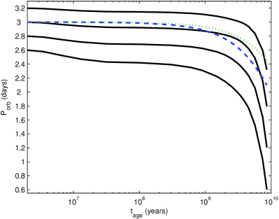
Figure 5: Change in the orbital period of a planet with a mass of one Jupiter mass around the Sun due to dynamical tides (for more details see the text).

III.2 The Star with a Mass of 1.5 $M_{\odot}$

In this subsection we present the results of our calculations of the overlap integrals and the change in orbital period for the star with a mass of one and a half solar masses. The star is considered from the time the protostar begins to collapse. This time is quite arbitrary and is $t=10^{-5}$ yr; the initial radius is $R=43.6R_{\odot}$. The initial metallicity of the star is $z=0.02$. At lifetimes of the star up to $t\approx 10^{6}$ yr it is completely convective ($N^{2}<0$). In such a star no lowfrequency g-modes are excited, and only the highfrequency f- and p-modes are present; therefore, the effective energy and angular momentum transfer from the orbit to the star will be suppressed. As the stellar age increases further, hydrogen burning begins at the stellar center and a radiative core appears ($N^{2}>0$), which begins to expand, encompassing progressively newer layers. The star has a well-defined convective envelope and a radiative core. The radiative region expands up to $R\approx 0.8R_{\odot}$ for the age $t=10^{7}$ yr. A fairly dense spectrum of low-frequency g-modes appears very rapidly in such a star.

At times $t\approx 2\times 10^{7}$ yr the stellar structure changes completely. A convective core appears in the star, while its envelope becomes completely radiative. The star abruptly contracts from a radius $R\approx 2.02R_{\odot}$ to $R\approx 1.5R_{\odot}$. The evolution time scales of the orbital parameters (2) increase sharply. The star passes from a solar-type star that has a radiative core and a convective envelope to a star with a convective core and a radiative envelope.

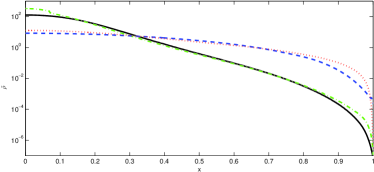
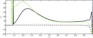
Figure 6: Density (a) and Brunt - V$\ddot{\rm a}$is$\ddot{\rm a}$l$\ddot{\rm a}$ frequency (b) for the star of one and a half solar masses versus radius for various times: the dashed, dotted, solid, and dash–dotted lines are for the ages $t=1.08\times 10^{2}$, $t=4.60\times 10^{6}$, $t=1.36\times 10^{8}$, and $t=1.47\times 10^{9}$ yr, respectively.

In Fig. 6 the stellar density and Brunt - V$\ddot{\rm a}$is$\ddot{\rm a}$l$\ddot{\rm a}$ frequency are plotted against radius for various times. From the figure we see how the central density increased as the star contracted. It can be seen from the figure for the Brunt - V$\ddot{\rm a}$is$\ddot{\rm a}$l$\ddot{\rm a}$ frequency that the star was initially completely convective (dashed curve) and subsequently a solar-type one (the envelope was convective, and the core was radiative; the dotted curve). At the subsequent times the star has a more complex structure, the core becomes convective, and the envelope is completely radiative (solid curve). A thin convective envelope then again appears in its envelope (dash–dotted curve).

Figure 7: Brunt - V$\ddot{\rm a}$is$\ddot{\rm a}$l$\ddot{\rm a}$ frequency versus radius for the star of one and a half solar masses for the age $t=1.47\times 10^{9}$ yr: the solid, dashed, and dash-dotted lines indicate the total Brunt - V$\ddot{\rm a}$is$\ddot{\rm a}$l$\ddot{\rm a}$ frequency $N^{2}$, the structural part $N^{2}_{\rm st}$, and the compositional part $N^{2}_{\rm com}$, respectively.

Figure 7 shows the Brunt - V$\ddot{\rm a}$is$\ddot{\rm a}$l$\ddot{\rm a}$ frequency as well as its structural and compositional parts. It follows from the figure that the compositional part makes the greatest contribution at the boundary between the convective and radiative regions.

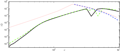
Figure 8: Overlap integrals versus frequency for the star of one and a half solar masses: the dashed, dotted, solid, and dash–dotted lines are for the ages $t=1.08\times 10^{2}$, $t=4.60\times 10^{6}$, $t=1.36\times 10^{8}$, and $t=1.47\times 10^{9}$ yr, respectively.

The overlap integrals are plotted against frequency in Fig. 8. The dashed line does not extend to the lowfrequency part of the spectrum, because the star at this time is completely convective ($N^{2}<0$). It can also be seen from the figure that the absolute value of the overlap integrals rapidly drops by more than two orders of magnitude as the star’s lifetime increases. Such catastrophic changes are due to the change in stellar structure. In the high-frequency part the absolute value of the overlap integrals increases by an order of magnitude, and characteristic kinks appear in the spectrum.

Figure 9 plots the change in the orbital period (in days) of a planet with a mass of one Jupiter mass around the star of one and a half solar masses with time (in years). The stellar evolutionmodels for which the overlap integrals were calculated are presented in Table 2. Equation (2) was integrated over time from $t\approx 1.98\times 10^{7}$ to $t\approx 2.24\times 10^{9}$ yr. For such a stellar lifetime interval the g-mode spectrum is sufficiently dense. The initial orbital periods of the planet around the Sun are $P_{\rm orb}=1.2,1.3,1.4,2,2.5,3$ days (solid curves). It follows from the figure that all planets with a mass equal to one Jupiter mass and with an initial orbital period of 2 days or shorter will fall onto the star in the main-sequence lifetime of the star. A planet with the initial orbital period $P_{\rm orb}=2$ days will fall onto the star, while a planet with the initial orbital period $P_{\rm orb}=2.5$ days will reduce its orbital period to $P_{\rm orb}=1.9$ days in the main-sequence lifetime of the star. The dashed curve indicates the change in orbital period without allowance for the stellar evolution. The time scale of the orbital change was taken at the star’s lifetime $t=7.82\times 10^{8}$ yr. It can be seen from Fig. 9 that the planet does not fall onto the star in the mainsequence lifetime of the star without allowance for its evolution.

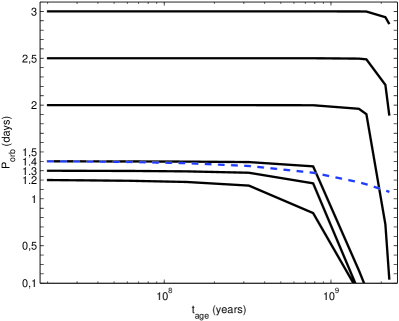
Figure 9: Change in the orbital period of a planet with a mass of one Jupiter mass around the star of one and a half solar masses due to dynamical tides (for more details see the text).

III.3 The Star with a Mass of 2$M_{\odot}$

The last star that we will consider is the star with a mass of two solar masses. The time the protostar begins to collapse is $t\approx 10^{-5}$ yr, the initial stellar radius is $R=57.4R_{\odot}$, and the stellar metallicity is $z=0.02$. At initial times up to $t\approx 3\times 10^{5}$ yr the star is completely convective ($N^{2}<0$). No low-frequency g-modes are excited; only the high-frequency f- and p-modes are present. The dynamical tides play no significant role in such a star. However, as the star evolves further, at times $t\approx 3\times 10^{5}$ yr a radiative region (radiative core) appears in the star, which begins to expand. The low-frequency g-modes are well excited in this region ($N^{2}>0$), and the dynamical tides begin to play an increasingly significant role as the star evolves further. Such a star resembles solartype stars that have a radiative core and a convective envelope. The radiative region expands quite rapidly, and this region almost reaches the stellar surface $R=0.987R_{\odot}$ already at times $t\approx 5.7\times 10^{6}$ yr. The star becomes almost completely radiative; the Brunt - V$\ddot{\rm a}$is$\ddot{\rm a}$l$\ddot{\rm a}$ frequency in the entire region becomes positive ($N^{2}>0$) in the entire region, except for the stellar surface. A sufficiently dense g-mode spectrum is generated in such a star. In Fig. 10 the stellar density and Brunt - V$\ddot{\rm a}$is$\ddot{\rm a}$l$\ddot{\rm a}$ frequency are plotted against radius for various times.

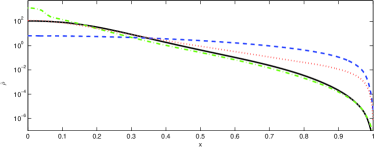
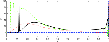
Figure 10: Density (a) and Brunt - V$\ddot{\rm a}$is$\ddot{\rm a}$l$\ddot{\rm a}$ frequency (b) for the star of two solar masses versus radius for various times: the dashed, dotted, solid, and dash–dotted lines are for the ages $t=1.49\times 10^{5}$, $t=4.54\times 10^{6}$, $t=9.50\times 10^{7}$, and $t=9.09\times 10^{8}$, respectively.

As the lifetime increases further ($t>5.8\times 10^{6}$ yr), a convective core ($N^{2}<0$) appears in the star, which begins to expand as the star evolves. The compositional part of the Brunt - V$\ddot{\rm a}$is$\ddot{\rm a}$l$\ddot{\rm a}$ frequency $N^{2}_{\rm com}$ begins to play an increasingly large role at the boundary between the convective and radiative regions (Fig. 11).

The stellar structure does not undergo significant changes as the lifetime increases further. Only the convective core evolves. Initially, the convective region expands, and then its expansion is replaced by contraction (Fig. 10).

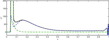
Figure 11: Brunt - V$\ddot{\rm a}$is$\ddot{\rm a}$l$\ddot{\rm a}$ frequency versus radius for the star of two solar masses for the age $t=9.09\times 10^{8}$ yr: the solid, dashed, and dash-dotted lines indicate the total Brunt - V$\ddot{\rm a}$is$\ddot{\rm a}$l$\ddot{\rm a}$ frequency $N^{2}$, the structural part $N^{2}_{\rm st}$, and the compositional part $N^{2}_{\rm com}$, respectively.

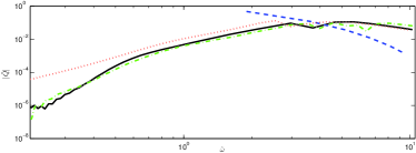
Figure 12: Overlap integrals versus frequency for the star of two solar masses: the dashed, dotted, solid, and dash-dotted lines are for the ages $t=1.49\times 10^{5}$, $t=4.54\times 10^{6}$, $t=9.50\times 10^{7}$, and $t=9.09\times 10^{8}$ yr, respectively.

The overlap integrals are plotted against frequency in Fig. 12. The dashed line does not extend to the low-frequency part of the spectrum, because the star at this time is completely convective ($N^{2}<0$). As the star’s lifetime increases, the absolute value of the overlap integral rapidly drops by more than an order of magnitude. Such catastrophic changes are due to the change in stellar structure. When the stellar structure undergoes no significant changes, the overlap integrals change gradually and insignificantly (see Fig. 12, the solid and dash-dotted lines).

Figure 13 plots the change in the orbital period (in days) of a planet with a mass of one Jupiter mass around the star of two solar masses with time (in years). The evolution models of the star of two solar masses for which the overlap integrals were calculated are presented in Table 3. Equation (2) was integrated over time from $t\approx 6.29\times 10^{6}$ to $t\approx 9.13\times 10^{8}$ yr. For such a stellar lifetime interval the g-mode spectrum is sufficiently dense. The initial orbital periods of the planet around the Sun were taken to be $P_{\rm orb}=1.5,1.6,1.7,2,2.5,3$ days (solid curves). It follows from the figure that all planets with a mass equal to one Jupiter mass and with an initial orbital period of 2 days or shorter will fall onto the star in the main-sequence lifetime of the star (Fig. 13). A planet with the initial orbital period $P_{\rm orb}=2.5$ days will reduce its orbital period only to $P_{\rm orb}\approx 2.35$ days in the main-sequence lifetime of the star. The dashed curve indicates the change in orbital period without allowance for the stellar evolution. The time scale of the orbital change was taken at the star’s lifetime $t=3.01\times 10^{8}$ yr. As can be seen from Fig. 13, the planet does not fall onto the star in the main-sequence lifetime of the star without allowance for its evolution. q

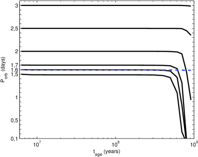
Figure 13: Change in the orbital period of a planet with a mass of one Jupiter mass around the star of two solar masses due to dynamical tides (for more details see the text).

Just as for the star of one and a half solar masses, the evolution time scales (3) of the planet decrease as the star begins to move off the main sequence. This is because the hydrogen reserves at the stellar center begin to be depleted, and the convective core becomes a helium one. This leads to an expansion of the star and, consequently, to an increase in the number of g-modes and the density of the spectrum, which leads to an increase in the pumping of orbital energy into the energy of stellar oscillations and to the fall of short-period planets onto the star.

IV CONCLUSIONS

We considered the change in the orbital period of a planet around a star with a mass of one, one and a half, and two solar masses. The behavior of the overlap integrals for these models as a function of the main-sequence lifetime of the star was analyzed. We showed that for the same star with a different structure during its evolution the overlap integrals could differ by two or more orders of magnitude.

We showed that all planets with a mass of one Jupiter mass that revolve around the Sun with an orbital period $P_{\rm orb}\approx 2.8$ days or shorter should fall onto the stellar surface in the main-sequence lifetime of the star. All planets with a mass of one Jupiter mass that revolve around the stars with a mass of one and a half and two solar masses with an orbital period $P_{\rm orb}\approx 2$ or shorter will fall onto the stellar surface in the main-sequence lifetime of the star. Such a fall may not occur without allowance for the evolution of the star itself.

These results qualitatively agree with the previous results from Bolmont and Mathis (2016) and Penev (2012). Calculations for the stellar models considered in this paper should be made for a more accurate quantitative estimate.

V ACKNOWLEDGMENTS

I am grateful to P.B. Ivanov who read the paper for a number of valuable remarks and to J. Papaloizou for a fruitful discussion. This work was financially supported by the Russian Foundation for Basic Research (project nos. 140200831, 150208476, 160201043), grant no. NSh-6595.2016.2 from the President of the Russian Federation for State Support of Leading Scientific Schools, and Program 7 of the Presidium of the Russian Academy of Sciences.

VI APPENDIX A

The system of equations describing the adiabatic perturbations in stars is written in dimensionless form (Christensen-Dalsgaard 1998):

$$\frac{dy_{1}}{dx} = -\left(\frac{2}{x}-\frac{\tilde{g}_{0}}{\tilde{c}^{2}_{0}}\right)y_{1}+$$

$$+ \left(\frac{1}{x}-\frac{\tilde{\omega}^{2}x}{\tilde{c}^{2}_{0}l(l+1)}\right)y_{2}+\frac{\tilde{g}_{0}}{\tilde{c}^{2}_{0}}y_{3},$$

$$\frac{dy_{2}}{dx} = \left(1-\frac{\tilde{N}^{2}_{0}}{\tilde{\omega}^{2}}\right)\frac{l(l+1)}{x}y_{1}-\frac{y_{2}}{x}+\frac{\tilde{N}^{2}_{0}}{\tilde{g}_{0}}y_{2}-$$

$$- \frac{l(l+1)\tilde{N}^{2}_{0}}{\tilde{\omega}^{2}x}y_{3},$$

$$\frac{dy_{3}}{dx} = \frac{y_{3}}{x}+\frac{y_{4}}{x},$$

$$\frac{dy_{4}}{dx} = \frac{3x\tilde{\rho}_{0}\tilde{N}^{2}_{0}}{\tilde{g}_{0}^{2}}y_{1}+\frac{3x^{2}\tilde{\omega}^{2}\tilde{\rho}_{0}}{\tilde{g}_{0}\tilde{c}^{2}_{0}l(l+1)}y_{2}$$ (14)

$$+ \left(\frac{l(l+1)}{x}-\frac{6\tilde{\rho}_{0}}{\tilde{g}_{0}}+\frac{3x\tilde{N}^{2}_{0}\tilde{\rho}_{0}}{\tilde{g}_{0}^{2}}\right)y_{3}-$$

$$- 2\left(-\frac{1}{x}+\frac{3\tilde{\rho}_{0}}{\tilde{g}_{0}}\right)y_{4},$$

where the following dimensionless variables are introduced: $x=\frac{r}{R}$ is the radius, $y_{1}=\frac{\xi_{r}}{R}$ is the radial perturbation, $y_{2}=\left(\frac{p^{{}^{\prime}}}{\rho_{0}}+\Phi^{{}^{\prime}}\right)\frac{l(l+1)}{\omega^{2}r^{2}}x=l(l+1)\frac{\xi_{h}}{R}$ is the horizontal perturbation, $y_{3}=x\frac{\Phi^{{}^{\prime}}}{g_{0}r}$ and $y_{4}=x^{2}\frac{d}{dx}\left(\frac{y_{3}}{x}\right)$ are the perturbations of the gravitational potential and its derivative, respectively. The subscript $0$ refers to an unperturbed quantity, and the prime ^′ refers to a perturbed quantity. A tilde over a quantity means that this quantity is dimensionless. The normalization is done as follows:

$$\omega^{2} = \frac{GM}{R^{3}}\tilde{\omega}^{2},\quad c^{2}_{0}=\frac{GM}{R}\tilde{c}^{2}_{0},\quad g_{0}=\frac{GM}{R^{2}}\tilde{g}_{0},$$

$$N^{2}_{0} = \frac{GM}{R^{3}}\tilde{N}^{2}_{0},\qquad\rho_{0}=\tilde{\rho_{0}}\frac{3M}{4\pi R^{3}},$$

$$p_{0} = \frac{GM^{2}}{4\pi R^{4}}\tilde{p}_{0},\qquad\tilde{c}^{2}_{0}=\frac{\Gamma\tilde{p}_{0}}{3\tilde{\rho}_{0}},$$ (15)

where $c^{2}$ is the sound speed squared, $p$ is the pressure, $\rho$ is the density, and $N^{2}$ is the Brunt - V$\ddot{\rm a}$is$\ddot{\rm a}$l$\ddot{\rm a}$ frequency squared. Four boundary conditions should be added to the four first-order differential equations. Two boundary conditions are specified at the stellar center, and the other two are specified on the stellar surface (Christensen-Dalsgaard 1998). The boundary conditions at the stellar center $x\rightarrow 0$ are

$$(l+1)y_{1}=y_{2},\quad y_{4}=(l-2)y_{3}.$$ (16)

The boundary conditions on the stellar surface $x\rightarrow 1$ are

$$y_{2}=\frac{l(l+1)}{\tilde{\omega}^{2}}(y_{1}+y_{3}),\qquad ly_{3}=-y_{4}.$$ (17)

There exists the Cowling (1941) approximation, in which the perturbed gravitational potential is neglected, to investigate the low-frequency g-modes. This approximation holds good and simplifies considerably the system of equations for the adiabatic perturbations (14). In the Cowling approximation the system of equations (14) will be rewritten in a simpler form:

$$\frac{dy_{1}}{dx} = -\left(\frac{2}{x}-\frac{\tilde{g}_{0}}{\tilde{c}^{2}_{0}}\right)y_{1}+\left(\frac{1}{x}-\frac{\tilde{\omega}^{2}x}{\tilde{c}^{2}_{0}l(l+1)}\right)y_{2},$$

$$\frac{dy_{2}}{dx} = \left(1-\frac{\tilde{N}^{2}_{0}}{\tilde{\omega}^{2}}\right)\frac{l(l+1)}{x}y_{1}-\frac{y_{2}}{x}+\frac{\tilde{N}^{2}_{0}}{\tilde{g}_{0}}y_{2}.$$ (18)

In the Cowling approximation the system of equations (18) ceases to depend explicitly on the stellar density. Thus, in the low-frequency limit the radial and horizontal displacements do not depend on the stellar density. In contrast, the overlap integrals (1) directly depend on the density. In the Cowling approximation not four but two boundary conditions should be added to the system of equations (18). One boundary condition is specified at the stellar center, and the other one is specified on the stellar surface. The boundary condition at the stellar center $x\rightarrow 0$ is

$$(l+1)y_{1}=y_{2}.$$ (19)

The boundary condition on the stellar surface $x\rightarrow 1$ is

$$y_{2}=\frac{l(l+1)}{\tilde{\omega}^{2}}y_{1}.$$ (20)

To determine the eigenfrequency spectrum of the system of equations (14) or (18), this system should be redefined. This requires that the determinant composed of the eigenfunctions of the system of equations (14) or (18) be equal to zero. This will hold only for some frequencies (eigenfrequencies) of the system of equations (14) or (18), which determines the perturbation spectrum.

VII APPENDIX B

The tables present the models for which the overlap integrals (1) and the evolution time scales of the orbital parameters (2) were calculated. The notation is as follows: $t$ is the time in years, $R$ is the radius measured in solar radii, $L$ is the luminosity measured in solar luminosities, $T_{eff}$ is effective surface temperature measured in Kelvins, h1 is the hydrogen mass fraction at the stellar center, and $\rho_{m}=\frac{3M}{4\pi R^{3}}$ is the mean stellar density measured in $g/cm^{3}$.

Table 1: The models used to calculate the characteristic orbital parameters for the Sun

t	R/$R_{\odot}$	L/$L_{\odot}$	$T_{eff}\times 10^{3}$	$h_{1}$	$\rho_{m}$
1.46$\times 10^{6}$	2.02	1.42	4.43	0.7	0.17
1.88$\times 10^{6}$	1.88	1.20	4.42	0.7	0.21
2.38$\times 10^{6}$	1.75	1.02	4.39	0.7	0.26
3.50$\times 10^{6}$	1.56	0.79	4.35	0.7	0.37
6.79$\times 10^{6}$	1.30	0.53	4.31	0.7	0.64
1.31$\times 10^{7}$	1.12	0.44	4.45	0.7	1.00
3.19$\times 10^{7}$	0.99	0.90	5.65	0.7	1.45
5.26$\times 10^{7}$	0.88	0.69	5.62	0.7	2.07
1.03$\times 10^{8}$	0.88	0.70	5.63	0.7	2.07
3.03$\times 10^{8}$	0.89	0.72	5.64	0.68	2.00
6.03$\times 10^{8}$	0.89	0.73	5.65	0.66	2.00
9.03$\times 10^{8}$	0.90	0.75	5.66	0.64	1.94
1.50$\times 10^{9}$	0.91	0.78	5.68	0.59	1.87
2.00$\times 10^{9}$	0.92	0.81	5.70	0.55	1.81
2.50$\times 10^{9}$	0.94	0.84	5.71	0.51	1.70
3.04$\times 10^{9}$	0.95	0.87	5.73	0.47	1.65
3.50$\times 10^{9}$	0.96	0.91	5.74	0.43	1.60
4.03$\times 10^{9}$	0.98	0.95	5.75	0.39	1.50
4.40$\times 10^{9}$	0.99	0.98	5.76	0.36	1.45
4.50$\times 10^{9}$	1.00	0.98	5.76	0.35	1.41
4.57$\times 10^{9}$	1.00	0.99	5.76	0.34	1.41
4.61$\times 10^{9}$	1.00	0.99	5.77	0.34	1.41
5.70$\times 10^{9}$	1.04	1.09	5.80	0.24	1.25
7.44$\times 10^{9}$	1.13	1.30	5.81	0.08	0.98
8.61$\times 10^{9}$	1.21	1.48	5.79	0.002	0.80

Table 2: The models used to calculate the characteristic orbital parameters for the star of one and a half solar masses

t	R/$R_{\odot}$	L/$L_{\odot}$	$T_{eff}\times 10^{3}$	$h_{1}$	$\rho_{m}$
1.00$\times 10^{-5}$	43.6	782	4.62	0.7	2.55$\times 10^{-5}$
5.37$\times 10^{-5}$	43.6	765	4.60	0.7	2.55$\times 10^{-5}$
1.49$\times 10^{-4}$	43.6	737	4.56	0.7	2.55$\times 10^{-5}$
4.85$\times 10^{-4}$	43.5	650	4.42	0.7	2.57$\times 10^{-5}$
1.06$\times 10^{-3}$	43.5	574	4.49	0.7	2.57$\times 10^{-5}$
5.67$\times 10^{-3}$	43.3	417	3.97	0.7	2.61$\times 10^{-5}$
1.18$\times 10^{-2}$	43.3	394	3.91	0.7	2.61$\times 10^{-5}$
5.10$\times 10^{-2}$	43.2	386	3.89	0.7	2.63$\times 10^{-5}$
1.06$\times 10^{-1}$	43.1	377	3.88	0.7	2.64$\times 10^{-5}$
5.46$\times 10^{-1}$	43.0	366	3.86	0.7	2.66$\times 10^{-5}$
1.13	42.8	362	3.85	0.7	2.70$\times 10^{-5}$
5.84	42.6	358	3.85	0.7	2.74$\times 10^{-5}$
1.01$\times 10$	42.5	357	3.85	0.7	2.76$\times 10^{-5}$
5.21$\times 10$	41.7	346	3.86	0.7	2.92$\times 10^{-5}$
1.08$\times 10^{2}$	40.6	333	3.87	0.7	3.16$\times 10^{-5}$
5.56$\times 10^{2}$	34.7	261	3.94	0.7	5.07$\times 10^{-5}$
1.09$\times 10^{3}$	30.5	215	4.01	0.7	7.46$\times 10^{-5}$
4.64$\times 10^{3}$	20.1	113	4.20	0.7	2.61$\times 10^{-4}$
1.39$\times 10^{4}$	13.6	61.1	4.37	0.7	8.42$\times 10^{-4}$
5.31$\times 10^{4}$	8.26	26.8	4.57	0.7	3.8$\times 10^{-3}$
1.06$\times 10^{5}$	6.37	17.2	4.66	0.7	8.2$\times 10^{-3}$
4.28$\times 10^{5}$	3.82	6.90	4.79	0.7	3.8$\times 10^{-2}$
8.81$\times 10^{5}$	2.96	4.22	4.81	0.7	8.2$\times 10^{-2}$
1.31$\times 10^{6}$	2.58	3.23	4.82	0.7	0.12
3.17$\times 10^{6}$	1.97	1.95	4.86	0.7	0.28
4.60$\times 10^{6}$	1.80	1.77	4.97	0.7	0.36
7.38$\times 10^{6}$	1.70	2.10	5.32	0.7	0.43
8.62$\times 10^{6}$	1.75	2.61	5.54	0.7	0.40
1.06$\times 10^{7}$	2.02	4.67	5.98	0.7	0.26
1.98$\times 10^{7}$	1.53	4.90	6.96	0.7	0.59
3.18$\times 10^{7}$	1.47	4.81	7.05	0.7	0.67
5.34$\times 10^{7}$	1.47	4.82	7.06	0.69	0.67
6.17$\times 10^{7}$	1.47	4.82	7.06	0.69	0.67
1.36$\times 10^{8}$	1.48	4.88	7.06	0.67	0.65
3.22$\times 10^{8}$	1.51	5.04	7.04	0.63	0.61
7.82$\times 10^{8}$	1.61	5.42	6.94	0.53	0.51
1.47$\times 10^{9}$	1.86	5.91	6.61	0.30	0.33
1.63$\times 10^{9}$	1.93	5.99	6.51	0.24	0.29
2.12$\times 10^{9}$	2.16	6.98	6.38	6.8$\times 10^{-3}$	0.21
2.24$\times 10^{9}$	2.46	8.79	6.35	5.6$\times 10^{-11}$	0.14

Table 3: The models used to calculate the characteristic orbital parameters for the star of two solar masses

t	R/$R_{\odot}$	L/$L_{\odot}$	$T_{eff}\times 10^{3}$	$h_{1}$	$\rho_{m}$
$10^{-5}$	57.4	1170	4.46	0.7	1.49$\times 10^{-5}$
4.55$\times 10^{-1}$	56.4	633	3.86	0.7	1.57$\times 10^{-5}$
3.35$\times 10^{2}$	47.3	483	3.94	0.7	2.67$\times 10^{-5}$
1.37$\times 10^{3}$	35.3	311	4.08	0.7	6.42$\times 10^{-5}$
7.83$\times 10^{3}$	19.8	128	4.37	0.7	3.64$\times 10^{-5}$
3.49$\times 10^{4}$	11.3	52.5	4.63	0.7	2.0$\times 10^{-3}$
1.49$\times 10^{5}$	6.51	21.0	4.85	0.7	1.02$\times 10^{-2}$
3.07$\times 10^{5}$	4.96	13.2	4.94	0.7	2.31$\times 10^{-2}$
6.37$\times 10^{5}$	3.81	8.18	5.01	0.7	5.10$\times 10^{-2}$
1.36$\times 10^{6}$	2.97	5.30	5.09	0.7	0.108
3.13$\times 10^{6}$	2.51	4.82	5.40	0.7	0.179
4.54$\times 10^{6}$	2.99	9.49	5.86	0.7	0.106
5.21$\times 10^{6}$	3.26	14.6	6.25	0.7	8.15$\times 10^{-2}$
5.68$\times 10^{6}$	2.99	19.5	7.02	0.7	0.106
6.29$\times 10^{6}$	2.36	23.8	8.31	0.7	0.215
8.56$\times 10^{6}$	1.74	18.9	9.14	0.7	0.536
9.59$\times 10^{6}$	1.65	16.8	9.12	0.7	0.628
1.01$\times 10^{7}$	1.64	16.6	9.11	0.69	0.640
1.53$\times 10^{7}$	1.63	16.4	9.12	0.69	0.652
2.26$\times 10^{7}$	1.63	16.4	9.12	0.69	0.652
3.78$\times 10^{7}$	1.64	16.5	9.10	0.69	0.640
5.07$\times 10^{7}$	1.64	16.5	9.08	0.68	0.640
6.92$\times 10^{7}$	1.66	16.6	9.05	0.67	0.62
9.50$\times 10^{7}$	1.68	16.7	9.02	0.66	0.6
1.24$\times 10^{8}$	1.70	16.9	8.98	0.64	0.57
2.15$\times 10^{8}$	1.77	17.4	8.86	0.60	0.51
3.01$\times 10^{8}$	1.85	17.9	8.74	0.55	0.45
4.06$\times 10^{8}$	1.96	18.6	8.57	0.48	0.37
4.98$\times 10^{8}$	2.08	19.2	8.39	0.42	0.31
6.11$\times 10^{8}$	2.26	20.0	8.12	0.33	0.24
7.02$\times 10^{8}$	2.45	20.5	7.85	0.25	0.19
8.04$\times 10^{8}$	2.75	20.9	7.45	0.15	0.14
9.09$\times 10^{8}$	2.76	25.5	7.81	2.6$\times 10^{-3}$	0.13
9.13$\times 10^{8}$	2.78	27.8	7.95	2.2$\times 10^{-4}$	0.13

References

- (1) P. Hut, Astron.Astrophys. 99, 126 (1981).
- (2) Zahn, Astron. Astrophys. 57, 383 (1977).
- (3) W.H. Press, S.A. Teukolsky, Astrophys.J. 213, 183 (1977).
- (4) P.B. Ivanov, I.D. Novikov, Astrophysic.J. 549, 467 (2001).
- (5) F.A. Rasio, et.al. Astrophys.J. 470, 1187 (1996).
- (6) K. Penev, et.al. Astrophys.J. 751, 96 (2012).
- (7) E. Bolmont, S. Mathis, ArXiv:1603.06268 [astro-ph].
- (8) P.B. Ivanov, J.C.B. Papaloizou, S.V. Chernov, MNRAS 432, 2339 (2013).
- (9) S.V. Chernov, J.C.B. Papaloizou, P.B. Ivanov, MNRAS 434, 1079 (2013).
- (10) P.B. Ivanov, J.C.B. Papaloizou, MNRAS 347, 437 (2004).
- (11) P.B. Ivanov, J.C.B. Papaloizou, MNRAS 353, 1161 (2004).
- (12) P.B. Ivanov, J.C.B. Papaloizou, MNRAS 407, 1609 (2010).
- (13) J.C.B. Papaloizou, P.B. Ivanov, MNRAS 407, 1631 (2010).
- (14) A.F. lanza, S. Mathis, ArXiv:1606.08623 [astro-ph].
- (15) J. Winn, D. Fabrycky, Annual Rev. Astron. Astrophys. 53, 409 (2015).
- (16) G. Ogilvie, Annual Rev. Astron. Astrophys. 52, 171 (2014).
- (17) A. Brucalassi, et.al. Astron. Astrophys. 561, L9 (2014).
- (18) N.N. Weinberg, et.al. Astrophys.J. 751, 136 (2012).
- (19) R. Essick, N.N. Weinberg, Astrophys.J. 816, 21 (2016).
- (20) J.C.B. Papaloizou, P.B. Ivanov, MNRAS 364, L66 (2005).
- (21) P.B. Ivanov, J.C.B. Papaloizou, MNRAS 376, 682 (2007).
- (22) T.G. Cowling, MNRAS 101,367 (1941).
- (23) Zahn, Astron. Astrophys. 4, 452 (1970).
- (24) A. Rocca, Astron. Astrophys. 175, 81 (1987).
- (25) Zahn, Astron. Astrophys. 41, 329 (1975).
- (26) J. Christensen-Dalsgaard, Lecture notes on stellar oscillations, 4th edn. (1998).
- (27) P. Brassard, G. Fontaine, F. Wesemael, S.D. Kawaler, M. Tassoul, Astrophys. J. 367, 601 (1991).
- (28) B. Paxton, et.al. Astrophys.J.Supp. 192, 3 (2011).
- (29) B. Paxton, et.al. Astrophys.J.Supp. 208, 4 (2013).
- (30) B. Paxton, et.al. Astrophys.J.Supp. 220, 15 (2015).
- (31) M. Steffen, Astron. Astrophys. 239, 443 (1990).