Spin-helix states in the $XXZ$ spin chain with strong dissipation

Abstract

We investigate the nonequilibrium steady state (NESS) in an open quantum XXZ chain attached at the ends to polarization baths with unequal polarizations. Using the general theory developed in [2], we show that in the critical $XXZ$ $|\Delta|<1$ easy plane case, the steady current in large systems under strong driving shows resonance-like behaviour, by an infinitesimal change of the spin chain anisotropy or other parameters. Alternatively, by fine tuning the system parameters and varying the boundary dissipation strength, we observe a change of the NESS current from diffusive (of order $1/N$, for small dissipation strength) to ballistic regime (of order 1, for large dissipation strength). This drastic change results from an accompanying structural change of the NESS, which becomes a pure spin-helix state characterized by a winding number which is proportional to the system size. We calculate the critical dissipation strength needed to observe this surprising effect.

• March 5, 2024

The $XXZ$ Heisenberg spin chain is a paradigmatic model in statistical mechanics. Its remarkable properties are long known in thermodynamic equilibrium [3, 4]. Recently, it was shown that also in a nonequilibrium setting, under a non-coherent boundary driving, the $XXZ$ chain retains many remarkable properties. An interesting strongly nonequilibrium setup of the problem occurs when a coherent evolution in the bulk is accompanied by a non-coherent local boundary driving, which tends to polarize the boundary spins along two different directions. If the boundary baths do not match, the system experiences a gradient of magnetization which leads to nonzero currents, even in the steady state. A schematic setup of the model is shown in Fig. 1. Note that the alignment of the boundary spins to the respective baths cannot be made perfect due to quantum fluctuations, except for the so-called Zeno limit, when the boundary dissipation is infinitely strong. An interplay between coherent bulk effects and incoherent boundary couplings results in the nontrivial scaling properties of the nonequilibrium steady state (NESS) characteristics (the currents, density profiles, many-point correlations, etc.), which can be distinguished as different phases of criticality of the $XXZ$ model [5, 6, 7].

Precise structure of the NESS for large systems and arbitrary mismatch of boundary polarizations is out of reach because the complexity of the problem grows exponentially with the system size $N$. From the general setup of the problem one would naively expect the NESS magnetization profile to interpolate between the left and right boundary as depicted in Fig. 1. A few solvable cases, for which the NESS can be found analytically, [8] suggest that the system properties essentially depend on the phases of criticality of the $XXZ$ model, characterized by the value of the spin exchange anisotropy $\Delta$, while the NESS within each phase separately varies regularly and smoothly.

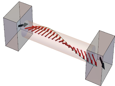
Figure 1: Schematic setup of a chain of spins attached to two fully polarizing boundary reservoirs. The chain has $N=20$ spins and we chose boundary conditions $\theta_{L}=\theta_{R}=0.4$, $\varphi_{L}=0$, $\varphi_{R}=4$.

In the present communication we demonstrate that, contrary to the expectations, the regular analytic behaviour of the NESS breaks down in a seemingly innocent and natural situation when the boundary driving is combined with an arbitrary spin-exchange anisotropy. We find that for a set of fine-tuned values of the anisotropy, various characteristics of the NESS, e.g., the magnetization current, may change dramatically, by orders of magnitude, and from monotonic behaviour to strongly nonmonotonic, provided that the dissipative strength $\Gamma$ becomes sufficiently large. For these special anisotropy values, and in their proximity as well, a structural transition in the NESS occurs, from a spatially smooth local magnetization profile interpolating between the boundary baths (small $k$ in the Fourier space), to a rigid quasi-periodic structure of spins corresponding to large $k$ values, arranged in a helix. Such a drastic structural transition naturally entails a singular behaviour of the NESS. Remarkably, spin-helix state is a pure state, which is rather unusual for a many-body interacting quantum system dissipatively coupled to an external bath. Detuning the anisotropy or lowering the dissipation strength below a threshold value makes the spin-helix structure to relax back to a smooth profile. The set of critical anisotropies, at which the structural transitions to spin-helix state occur, becomes dense on the segment $[-1,1]$ in the limit of large system size $N$.

The plan of the paper is as follows. We introduce the model and various properties of interest in Sec. 1. In Sec. 2 we review the conditions under which the pure NESS is achieved in the Zeno limit. In Sec. 3 the convergence to an atypical NESS for finite dissipative strength is quantified, while in Sec. 4 we characterize the points where this convergence fails. We discuss two possible experimental scenarios in Sec. 5 and, finally, in Sec. 6 we draw our conclusions.

1 Model

We consider an open $XXZ$ chain coupled dissipatively to boundary reservoirs, described via the Lindblad master equation [9, 10, 11]

$$\frac{\partial\rho}{\partial t}=-\frac{i}{\hbar}\left[H,\rho\right]+\sum_{\alpha}L_{\alpha}\rho L^{\dagger}_{\alpha}-\frac{1}{2}\left(L_{\alpha}^{\dagger}L_{\alpha}\rho+\rho L_{\alpha}^{\dagger}L_{\alpha}\right),$$ (1)

where $H$ is the spin $1/2$ Heisenberg Hamiltonian with a partial anisotropy along the $Z$-axis

$$H_{XXZ} =\sum_{j=1}^{N-1}h_{j,j+1}^{XXZ}=\sum_{j=1}^{N-1}J\left(\sigma_{j}^{x}\sigma_{j+1}^{x}+\sigma_{j}^{y}\sigma_{j+1}^{y}+\Delta\left(\sigma_{j}^{z}\sigma_{j+1}^{z}-I\right)\right).$$ (2)

The parameter $\Delta$ describes the $Z$-anisotropy. The Lindblad operators are chosen so as to target completely polarized states of the leftmost and rightmost spins (spins number 1 and number $N$, respectively). We parametrize the targeted boundary polarizations by polar and azimuthal angles $\theta_{L},\varphi_{L}$ on the left end of the chain and $\theta_{R},\varphi_{R}$ on its right end. We consider only two Lindblad operators, $L_{1},L_{2}$, the first one being

$$L_{1}=\frac{\sqrt{\Gamma}}{2}\left(-\sin\theta_{L}\sigma_{1}^{z}+(1+\cos\theta_{L})e^{-i\varphi_{L}}\sigma_{1}^{+}+(-1+\cos\theta_{L})e^{i\varphi_{L}}\sigma_{1}^{-}\right),$$ (3)

where $\sigma^{\alpha}$, $\alpha=x,y,z$, are Pauli matrices, lower indices denote the embeddings in the physical space, and $\sigma^{\pm}=(\sigma^{x}\pm i\sigma^{y})/2$. The second Lindblad operator, $L_{2}$, is obtained from Eq. (3) by the substitutions $\sigma_{1}^{\alpha}\rightarrow\sigma_{N}^{\alpha}$, $\theta_{L}\rightarrow\theta_{R}$, $\varphi_{L}\rightarrow\varphi_{R}$. It can be straightforwardly verified, that the pure one-site state $\rho_{L}=\left|\psi_{1}\right\rangle\left\langle\psi_{1}\right|$, with $\left\langle\psi_{1}\right|=\langle\cos(\theta_{L}/2)e^{-i\varphi_{L}/2},\sin(\theta_{L}/2)e^{i\varphi_{L}/2}|$, is a dark state of $L_{1}$, i.e., $L_{1}\left|\psi_{1}\right\rangle=0$. In the absence of the coherent evolution term in Eq. (1), the left boundary spin relaxes to a state $\rho_{L}=\left|\psi_{1}\right\rangle\left\langle\psi_{1}\right|=\frac{1}{2}\vec{l}_{L}\vec{\sigma}_{1}$, with $\vec{l}_{L}=(\sin\theta_{L}\cos\varphi_{L},\sin\theta_{L}\sin\varphi_{L},\cos\theta_{L})$, with a characteristic time $\tau=\Gamma^{-1}$. An analogous statement holds for the rightmost spin, which (in the absence of the coherent evolution) gets polarized along the direction $\vec{l}_{R}=(\sin\theta_{R}\cos\varphi_{R},\sin\theta_{R}\sin\varphi_{R},\cos\theta_{R})$. A possible experimental protocol of repeating interactions leading to the density matrix evolution (1) (3) is discussed in [12]. It is clear that any non fully matching boundary conditions, $(\theta_{L},\varphi_{L})\neq(\theta_{R},\varphi_{R})$, introduces a boundary mismatch, and results in steady currents flowing through the chain. In particular, due to the spin-exchange anisotropy in $XY$-plane, the $Z$-component of the magnetization current $j^{z}$ is locally conserved.

In the following solvable cases, the NESS, namely, the time-independent solution of Eq. (1), is known analytically:

Collinear boundary driving along the anisotropy axis $\varphi_{L}=\varphi_{R}=0,\theta_{L}=0,\theta_{R}=\pi$ [7]. The steady magnetization current is ballistic in the critical regime $|\Delta|<1$, is exponentially small in the Ising-like case $|\Delta|>1$ and is subdiffusive in the isotropic case $\Delta=1$. For large $\Gamma$, the $Z$-component of the magnetization current $j^{z}$ vanishes due to quantum Zeno effect.

Non-collinear $XY$-plane boundary driving $\varphi_{L}=0,\varphi_{R}=\Phi,\theta_{L}=\theta_{R}=\pi/2$ and isotropic Heisenberg model $\Delta=1$ [13, 14]. In the isotropic case, all components of the magnetization current are conserved. The components $j^{x},j^{y}$ are subdiffusive and decrease for large $\Gamma$, due to quantum Zeno effect, while $j^{z}$ monotonically increases with $\Gamma$. The NESS-dependence on $\Gamma$ is regular and piecewise monotonic.

Non-collinear strong $XY$-plane boundary driving and fine-tuned anisotropy $\Delta$. It was suggested in [15], that for sufficiently strong dissipative coupling, the NESS becomes arbitrarily close to a pure state, which we shall call spin-helix state (SHS), in analogy to states appearing in two-dimensional electron systems with spin-orbit coupling [16, 17, 18], $\lim_{\Gamma\rightarrow\infty}\rho_{\mathrm{NESS}}(\Gamma)=\left|\Psi_{\mathrm{SHS}}\right\rangle\left\langle\Psi_{\mathrm{SHS}}\right|$, where

$$\left|\Psi_{\mathrm{SHS}}\right\rangle=2^{-\frac{N}{2}}\bigotimes_{k=1}^{N}\left(\begin{array}[]{c}e^{-\frac{i}{2}\varphi(k-1)}\\ e^{\frac{i}{2}\varphi(k-1)}\end{array}\right),$$ (4)

provided the states of the boundary spins match the boundary driving, namely, $\theta_{L}=\theta_{R}=\pi/2$, $\varphi_{L}=0,\varphi_{R}\equiv(N-1)\varphi=\Phi$, and the anisotropy $\Delta$ obeys

$$\Delta=\cos\varphi.$$ (5)

In the present situation, when the Lindblad operators (3) are targeting pure single-spin states, the spin-helix states (4) are obtained in an ideal Zeno regime $\Gamma\to\infty$. Note, however, that it is also possible to generate the same spin-helix states for finite dissipative strengths $\Gamma$, if fine-tuned mixed single-spin states at the boundaries are dissipatively targeted [19].

The spin-helix states (4) are quite remarkable in many respects. From the point of view of a dissipative dynamics, the creation of a pure quantum state via a dissipative action is a way to beat detrimental decoherence effects. From the point of view of spintronics, the state (4) carries an anomalously high ballistic magnetization current of order $1$, which is independent of the system size.

The existence of SHS in the Zeno limit at fine-tuned anisotropy (5) was guessed in [15] on the base of a necessary criterion and explicit calculation of the NESS for small system sizes. Here we revisit and systematically treat the SHS on the base of a general theory (which provides necessary and sufficient criteria for SHS existence, and also a convergence criterion) developed by us in [2]. We treat more general SHS,

$$\left|\Psi_{\mathrm{SHS}}\right\rangle=\bigotimes_{k=1}^{N}\left(\begin{array}[]{c}\cos(\frac{\theta}{2})e^{-\frac{i}{2}\varphi(k-1)}\\ \sin(\frac{\theta}{2})e^{\frac{i}{2}\varphi(k-1)}\end{array}\right),$$ (8)

which, as we shall see later, can be dissipatively generated in a boundary driven $XXZ$ spin chain by tuning the boundary conditions and the anisotropy. The state (8) describes a precession, along the chain, of the local spin around the $Z$-axis, forming a frozen spin wave structure, see Fig. 1 for an illustration, with constant twisting azimuthal angle difference $\varphi$ between two neighbouring spins. This is evident if we compute the expectation value of the local spin at site $n$

$$\left\langle\Psi_{\mathrm{SHS}}\right|\vec{\sigma}_{n}\left|\Psi_{\mathrm{SHS}}\right\rangle=(\sin\theta\cos\varphi(n-1),\sin\theta\sin\varphi(n-1),\cos\theta).$$ (9)

The local spin orientations obtained in a chain with $N=20$ spins and boundary conditions $\theta_{L}=\theta_{R}=0.4$, $\varphi_{L}=0$, $\varphi_{R}=4$ are shown in Fig. 1.

Note that fixed boundary polarizations $\varphi_{L}=0,\varphi_{R}=\Phi$ match not just one spin-helix state (8) with $\varphi(N-1)=\Phi$, but also those with $\varphi(N-1)=\Phi+2\pi$, $\varphi(N-1)=\Phi+4\pi$ etc., until $\varphi(N-1)=\Phi+(N-2)2\pi$. Thus, we shall also characterize a spin-helix state via a winding number $m=\lfloor(N-1)\varphi/(2\pi)\rfloor$, $\lfloor\cdot\rfloor$ being the integer part.

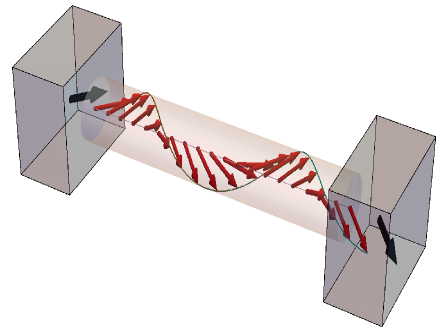
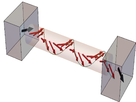
Figure 2: spin-helix states as in Fig. 1 but with winding numbers $m=1$ (top) and $m=2$ (bottom).

We will see in the following that the spin-helix states (8) constitute the points of resonance-like behaviour of the NESS, which becomes visible at large dissipation. In doing that, we shall answer some basic questions. How large must the dissipation strength be to reach the limiting spin-helix state with a predefined accuracy? To which extent the characteristics of the spin-helix state/states are atypical for given boundary mismatch? Can the resonance-like behaviour be detected in other features of the NESS? What happens if the system gets larger and larger, and, eventually, we reach the thermodynamic limit of infinitely long chains?

The characterization of several properties of the NESS prove to be useful for our later considerations.
(a) A measure of the purity. In fact, in driven Heisenberg spin chains with polarization targeting operators, a NESS can become pure, e.g., $\rho_{\mathrm{NESS}}=\left|\Psi_{\mathrm{SHS}}\right\rangle\left\langle\Psi_{\mathrm{SHS}}\right|$, where $\left|\Psi_{\mathrm{SHS}}\right\rangle$ is the spin-helix state (8), only in the Zeno limit. As a criterion for purity of a state $\rho$, we shall use both the von Neumann entropy, $S_{VNE}(\rho)=-\mathop{\mathrm{tr}}\limits(\rho\log_{2}\rho)$, as well as the alternative measure $\epsilon(\rho)=1-\mathop{\mathrm{tr}}\limits(\rho^{2})$.
(b) Steady currents of magnetization and of energy. Being a nonequilibrium steady state, the NESS is characterized by non-vanishing steady currents. The magnetization (spin) current operator in the $Z$-direction, $\hat{\jmath}_{n,n+1}$, is defined via a lattice continuity equation $\frac{d}{dt}\sigma_{n}^{z}=\hat{\jmath}_{n-1,n}-\hat{\jmath}_{n,n+1}$, where

$$\hat{\jmath}_{n,m}=J(\sigma_{n}^{x}\sigma_{m}^{y}-\sigma_{n}^{y}\sigma_{m}^{x}).$$ (10)

The energy current operator, $\hat{J}_{n}^{E}$, is defined analogously by $\frac{d}{dt}h_{n,n+1}=\hat{J}_{n}^{E}-\hat{J}_{n+1}^{E}$, where

$$\hat{J}_{n}^{E}=-\sigma_{n}^{z}\hat{\jmath}_{n-1,n+1}+\Delta(\hat{\jmath}_{n-1,n}\sigma_{n+1}^{z}+\sigma_{n-1}^{z}\hat{\jmath}_{n,n+1}).$$ (11)

(c) Finally, we need a cumulative function characterizing the density profile $\sigma_{n}^{\alpha}$, which probes the helix structure of the spins. To this end, we introduce a generalized structure factor (or, alternatively, a generalized discrete Fourier Transform (GFT)), via

$$\hat{f}_{m}(\Phi)=\frac{1}{M}\sum_{k=0}^{M-1}f_{k}e^{-i\varphi(m)k},$$ (12)

where

$$\varphi(m)=\frac{\Phi+2\pi m}{M},\qquad m=0,1,\dots,M-1.$$ (13)

Here, $M+1=N$ is the chain length, $0\leq\Phi<2\pi$ and $m$ is the winding number. For $\Phi=0$, Eq. (12) turns into the usual discrete Fourier Transform. The GFT shares similar properties with the usual Fourier Transform, e.g., the Parseval identity has the usual form

$$\sum_{m=0}^{M-1}|\hat{f}_{m}(\Phi)|^{2}=\frac{1}{M}\sum_{k=0}^{M-1}|f_{k}|^{2}.$$ (14)

A convenient quantity to look at is the GFT (12) of the one-point observables

$$f_{k-1}=\mathop{\mathrm{tr}}\limits((\sigma_{k}^{x}+i\sigma_{k}^{y})\rho),\qquad k=1,2,\dots,N-1,$$ (15)

which play the role of the usual Fourier harmonics. Indeed, for a spin-helix state with winding number $m_{0}$, we find $f_{k}=e^{i\varphi(m_{0})k}$.

The above quantities (a)-(c) are easily calculated for the stationary spin-helix state $\rho_{\mathrm{SHS}}=\left|\Psi_{\mathrm{SHS}}\right\rangle\left\langle\Psi_{\mathrm{SHS}}\right|$, where $\left|\Psi_{\mathrm{SHS}}\right\rangle$ is given by Eq. (8) with $\varphi=\varphi(m_{0})=(\Phi+2\pi m_{0})/(N-1)$, yielding

$$S_{VNE}(\rho_{\mathrm{SHS}}) =\epsilon(\rho_{\mathrm{SHS}})=0,$$ (16)

$$j^{z}(\rho_{\mathrm{SHS}}) =\mathop{\mathrm{tr}}\limits(\hat{\jmath}_{n,n+1}\rho_{\mathrm{SHS}})=J\sin\theta\sin\varphi(m_{0}),$$ (17)

$$J_{E}(\rho_{\mathrm{SHS}}) =\mathop{\mathrm{tr}}\limits(\hat{J}_{n}^{E}\rho_{\mathrm{SHS}})=0,$$ (18)

$$\hat{f}_{m}(\Phi) =\sin\theta\delta_{m,m_{0}},\qquad m=0,1,\dots,N-2.$$ (19)

We stress that the spin-helix state is realized as a NESS of the system only in the ideal limit $\Gamma\to\infty$. To see how the above quantities change in the physically more relevant situation of $\Gamma$ finite, consider first a simple yet demonstrative example. Figures 3 and 4 show the von Neumann entropy of the actual $\rho_{\mathrm{NESS}}$ and the corresponding steady-state magnetization current $j^{z}$ as a function of the anisotropy $\Delta$ for fixed $N$, $\theta$ and $\Phi$, for two, large and small values of the dissipation strength $\Gamma$ (for a quantification of the notions “large” and “small” see Sec. 3). The NESS is found solving numerically Eq. (1).

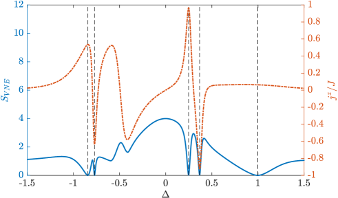
Figure 3: von Neumann entropy (solid blue line,left vertical scale) of the NESS and steady-state magnetization current (dot-dashed red line, right vertical scale) versus the anisotropy $\Delta$ for $\Gamma=1000$. The minima of $S_{VNE}$ correspond to almost pure spin-helix states with different winding numbers. The vertical dashed lines indicate the critical anisotropies of Eq. (20) obtained, from left to right, for $m=2,3,4,1,0$. System parameters: $N=6$, $\theta=\pi/2$, $\Phi=\pi/10$.

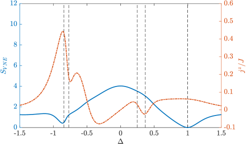
Figure 4: As in Fig. 3 for $\Gamma=10$.

For large $\Gamma$, in Fig. 3 we see that for values of the anisotropy $\Delta$ given by

$$\Delta_{\mathrm{cr}}(m,\Phi)=\cos\frac{\Phi+2\pi m}{N-1},\qquad m=0,1,\dots,N-2,$$ (20)

$\rho_{\mathrm{NESS}}$ becomes a pure state, namely, a spin-helix state with winding number $m$. For the same value of $\Gamma$, the steady-state magnetization current abruptly changes sign and amplitude in the region $\Delta\in[-1,1]$ depending on the value of $\sin\varphi(m)$. For small $\Gamma$, see Fig. 4, the above pure-state features fade away for both $S_{VNE}$ and $j^{z}$.

If the polarizations of the boundary spins of the chain differ slightly, as in the example shown in Figs. 3 and 4, where the boundary angle mismatch is $\Phi=\pi/10$, one would expect a steady magnetization current proportional to the bulk gradient $\Phi/(N-1)$. In fact, naively, one may assume that neighbouring spins $k,k+1$ are almost collinear in the steady state. This scenario indeed happens for small $\Gamma$, and, if $\Gamma$ is large, for $\Delta$ away from the critical values (20), where the spins arrange in a helix structure with angle between neighbouring spins $\varphi=(\Phi+2\pi m)/(N-1)$, $m=0,1,\dots,N-2$. On the other hand, at the critical values of $\Delta$ corresponding to winding numbers $m>0$, a resonance takes place with a drastic increase of the amplitude of the steady current $j^{z}$. As the system size grows, the magnetization current and the von Neumann entropy peaks become narrower and steeper.

To verify the existence of the helix structure of the spins in the regions near the critical values of the anisotropy, it is instructive to look at the GFT coefficients $\hat{f}_{m}$ of Eq. (12) as a function of the anisotropy. As shown in Figs. 5 and 6, the GFT coefficients $\hat{f}_{m}$ reach their absolute maxima exactly at the points $\Delta_{\mathrm{cr}}(m,\Phi)$, in agreement with the prediction of Eq. (19). This allow us to conclude that the pure states evidenced in Fig. 4 by the vanishing of $S_{VNE}$ are, in fact, the spin-helix states (8). Note that, for $\Gamma$ large, i.e., in Fig. 5, the amplitudes of the maxima of the coefficients $\hat{f}_{m}$ are independent of $m$ and coincide with the value $\sin\theta$ predicted by Eq.  (19).

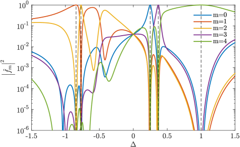
Figure 5: Generalized Fourier coefficients $\hat{f}_{m}$ versus the anisotropy $\Delta$ for $\Gamma=1000$. System parameters as in Fig. 3.

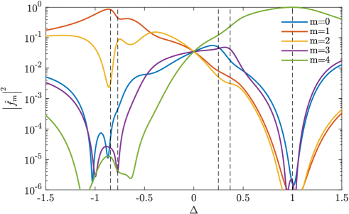
Figure 6: As in Fig. 5 for $\Gamma=10$.

2 Boundary driven $XXZ$ spin chain: criterion for NESS purity

In order for the NESS to be pure in the Zeno limit, we require an existence of a NESS expansion in powers of $1/\Gamma$,

$$\rho_{\rm{NESS}}(\Gamma) =\sum_{m=0}^{\infty}\frac{\rho^{(m)}}{\Gamma^{m}},$$ (21)

where the zeroth order term is a pure state,

$$\rho^{(0)} =\left|\Psi\right\rangle\left\langle\Psi\right|.$$ (22)

Consistency of the expansion (21) with the purity assumption (22) leads to restrictions for the effective Hamiltonian $H$. The general theory [2] predicts that, for boundary driven systems, in the Zeno limit a pure steady state $\rho_{\mathrm{NESS}}=\left|\Psi\right\rangle\left\langle\Psi\right|$ can be targeted, where $\left|\Psi\right\rangle=\left|\psi_{\mathrm{Zeno}}\right\rangle\otimes\left|\psi_{\mathrm{target}}\right\rangle$, with $\left|\psi_{\mathrm{Zeno}}\right\rangle\in\mathcal{H}_{0}$ and $\left|\psi_{\mathrm{target}}\right\rangle\in\mathcal{H}_{1}$, $\mathcal{H}_{0}$ being the Hilbert subspace where the dissipation (Lindblad operators) acts and $\mathcal{H}_{1}$ its complement to the whole Hilbert space, $\mathcal{H}=\mathcal{H}_{0}\otimes\mathcal{H}_{1}$. A necessary condition for this NESS purity to be achieved is that

$$H|\Psi\rangle=\lambda|\Psi\rangle+\kappa\left|\psi_{\mathrm{Zeno}}^{\perp}\right\rangle\otimes|\psi_{\mathrm{target}}\rangle,$$ (23)

where $\left|\psi_{\mathrm{Zeno}}^{\perp}\right\rangle\in\mathcal{H}_{0}$ is a state orthogonal to $\left|\psi_{\mathrm{Zeno}}\right\rangle$, $\kappa\neq 0$, and $\lambda$ is an arbitrary real constant. The criterion (23) gives a necessary condition, while two extra conditions must be checked to guarantee the convergence of the NESS to the targeted pure state $\left|\Psi\right\rangle$ in Zeno limit. These extra conditions will be discussed in sec.4.

The validity of the purity criterion (23) for the Heisenberg Hamiltonian with the boundary spins $1$ and $N$ attached to polarizing reservoirs, stems from the following property of the local Hamiltonian density $h_{j,j+1}^{XXZ}(\Delta)$, with $\Delta=\cos\varphi$,

$$h_{j,j+1}^{XXZ}(\cos\varphi)\left|\psi(\theta,\alpha)\right\rangle_{j}\otimes\left|\psi(\theta,\alpha+\varphi)\right\rangle_{j+1}=-iJ\sin\theta\sin\varphi$$

$$\qquad\times\left(\left|\psi^{\perp}(\theta,\alpha)\right\rangle_{j}\otimes\left|\psi(\theta,\alpha+\varphi)\right\rangle_{j+1}-\left|\psi(\theta,\alpha)\right\rangle_{j}\otimes\left|\psi^{\perp}(\theta,\alpha+\varphi)\right\rangle_{j+1}\right),$$ (24)

where the lower index in a state denotes the respective embedding and

$$\left|\psi(\theta,\alpha)\right\rangle=\binom{\cos\frac{\theta}{2}e^{-i\alpha/2}}{\sin\frac{\theta}{2}e^{i\alpha/2}},$$ (25)

$$\left|\psi^{\perp}(\theta,\alpha)\right\rangle=\binom{\sin\frac{\theta}{2}e^{-i\alpha/2}}{-\cos\frac{\theta}{2}e^{i\alpha/2}}.$$ (26)

It is simple to verify that Eq. (23) is satisfied with $\lambda=0,\kappa=-iJ\sqrt{2}\sin\theta\sin\varphi$, and

$$\left|\psi\right\rangle_{\mathrm{Zeno}}=\left|\psi(\theta,0)\right\rangle_{1}\otimes\left|\psi(\theta,\Phi)\right\rangle_{N},$$ (27)

$$\left|\psi\right\rangle_{\mathrm{Zeno}}^{\perp}=\frac{1}{\sqrt{2}}\left(\left|\psi^{\perp}(\theta,0)\right\rangle_{1}\otimes\left|\psi(\theta,\Phi)\right\rangle_{N}-\left|\psi(\theta,0)\right\rangle_{1}\otimes\left|\psi^{\perp}(\theta,\Phi)\right\rangle_{N}\right),$$ (28)

$$\left|\psi_{\mathrm{target}}\right\rangle=\bigotimes_{j=2}^{N-1}\left|\psi(\theta,(j-1)\varphi)\right\rangle_{j}.$$ (29)

Note that in the above three states we have $\alpha=0$ and $\varphi=(\Phi+2\pi m)/(N-1)$, with $m$ integer. We conclude that the stationary pure state approached in the Zeno limit (fully polarizing reservoirs), namely,

$$\left|\Psi\right\rangle=\bigotimes_{j=1}^{N}\left|\psi(\theta,(j-1)\varphi)\right\rangle_{j}.$$ (30)

is the spin-helix state anticipated in Eq. (8). It describes a “homogeneous” spin precession around the anisotropy axis $Z$ along the chain, with a constant polar angle $\theta$ and a monotonically increasing azimuthal angle $(j-1)\varphi$, $j=1,2,\dots,N$, matching the boundary values $(\sin\theta,0,\cos\theta)$ and $(\sin\theta\cos\Phi,\sin\theta\sin\Phi,\cos\theta)$. Indeed, the expectation value of the spin projection at site $j$ is

$$\langle\vec{\sigma}_{j}\rangle =\mathop{\mathrm{tr}}\limits\left(\left|\psi(\theta,(j-1)\varphi)\right\rangle\left\langle\psi(\theta,(j-1)\varphi)\right|\vec{\sigma}\right)$$

$$=(\sin\theta\cos(j-1)\varphi,\sin\theta\sin(j-1)\varphi,\cos\theta).$$ (31)

For $\theta=\pi/2$, we have the simpler helix-state of Eq. (4) describing spins which locally rotate entirely in the $XY$ plane.

Whereas the criterion (23) ensures that the NESS converges to the spin-helix pure state in the limit $\Gamma\to\infty$, the general theory developed in [2] allows us to quantify the speed of this convergence by establishing a characteristic dissipation as discussed in the next Section.

3 Convergence to the spin-helix state for finite dissipation strength

According to [2], we introduce an orthonormal basis $\left|e^{j}\right\rangle$ in the subspace ${\cal H}_{0}$ where dissipation acts and split the Hamiltonian $H$ with respect to this basis. In our present case ${\cal H}_{0}$ is the direct product of the local spin spaces corresponding to the sites $1$ and $N$,

$$H=\sum_{j=0}^{d_{0}-1}\sum_{k=0}^{d_{0}-1}H_{jk}=\sum_{j=0}^{d_{0}-1}\sum_{k=0}^{d_{0}-1}|e^{j}\rangle\langle e^{k}|\otimes h^{jk},$$ (32)

where $d_{0}=4$ is the dimension of ${\cal H}_{0}$. The first two basis vectors are chosen as $\left|e^{0}\right\rangle\equiv\left|\psi_{\mathrm{Zeno}}\right\rangle$ and $\left|e^{1}\right\rangle\equiv\left|\psi_{\mathrm{Zeno}}^{\perp}\right\rangle$, with $\left|\psi_{\mathrm{Zeno}}\right\rangle$ and $\left|\psi_{\mathrm{Zeno}}^{\perp}\right\rangle$ defined as in Eqs. (27) and (28), respectively. The other vectors of the basis are chosen as (lower indices denote the embedding)

$$\left|e^{2}\right\rangle =\frac{1}{\sqrt{2}}\left(\left|\psi^{\perp}(\theta,0)\right\rangle_{1}\left|\psi(\theta,\Phi)\right\rangle_{N}+\left|\psi(\theta,0)\right\rangle_{1}\left|\psi^{\perp}(\theta,\Phi)\right\rangle_{N}\right),$$ (33)

$$\left|e^{3}\right\rangle =\left|\psi^{\perp}(\theta,0)\right\rangle_{1}\left|\psi^{\perp}(\theta,\Phi)\right\rangle_{N}.$$ (34)

Having defined the basis in the ${\cal H}_{0}$, the coefficients $h^{jk}$ of the decomposition (32), which are operators in $\mathcal{H}_{1}$, are readily calculated as

$$h^{jk}=\mathop{\mathrm{tr}_{1,N}}\limits\left(\left(\left|e^{k}\right\rangle\left\langle e^{j}\right|I_{2,3,\dots,N-1}\right)H\right),$$ (35)

where $I_{2,3,\dots,N-1}$ is the identity operator in the space of spins $2,3,\dots,N-1$, and

$$\mathop{\mathrm{tr}_{1,N}}\limits({\cdot}) =\mathop{\mathrm{tr}_{N}}\limits(\mathop{\mathrm{tr}_{1}}\limits(\cdot)),$$ (36)

$$\mathop{\mathrm{tr}_{n}}\limits(\cdot) =\left(\left\langle+\right|\cdot\left|+\right\rangle\right)_{n}+\left(\left\langle-\right|\cdot\left|-\right\rangle\right)_{n},\qquad n=1,2,\dots,N,$$ (37)

where $\left|\pm\right\rangle$ are the eigenstates of $\sigma^{z}$.

Of special importance is the term $h^{00}$, which is the projection of the Hamiltonian $H$ on the state $\left|e^{0}\right\rangle$ targeted by the dissipation. In fact, we have $\mathcal{D}_{1}\left|e^{0}\right\rangle\left\langle e^{0}\right|=\mathcal{D}_{N}\left|e^{0}\right\rangle\left\langle e^{0}\right|=0$, where $\mathcal{D}_{1}$ and $\mathcal{D}_{N}$ are the dissipators associated to the Lindblad operators $L_{1}$ and $L_{N}$, e.g., $\mathcal{D}_{1}\rho=L_{1}\rho L_{1}^{\dagger}-\frac{1}{2}(L_{1}^{\dagger}L_{1}\rho+\rho L_{1}^{\dagger}L_{1})$. From Eq. (35) and after some algebra, we obtain

$$h^{00}=H^{\prime}+C_{++}(2,\theta,0)+C_{++}(N-1,\theta,\Phi),$$ (38)

$$H^{\prime}=\sum_{j=2}^{N-2}h^{XXZ}_{j,j+1}(\Delta),$$ (39)

$$C_{++}(m,\theta,\varphi)=\mathop{\mathrm{tr}_{m-1}}\limits\left(\left(\left|\psi(\varphi)\right\rangle\left\langle\psi(\varphi)\right|\right)_{m-1}h^{XXZ}_{{m-1},m}\right)$$

$$\phantom{C_{++}(m,\theta,\varphi)}=J(\sin\theta(e^{i\varphi}\sigma^{-}_{m}+e^{-i\varphi}\sigma^{+}_{m})+\Delta\sigma^{z}_{m}\cos\theta-\Delta I_{2,3,\dots,N-1}),$$ (40)

where $h^{XXZ}_{j,j+1}$ are the local energy densities of the $XXZ$ Hamiltonian (2) and $\sigma^{\alpha}_{m}=I_{2,3,\dots,m-1}\otimes\sigma^{\alpha}\otimes I_{m+1,\dots,N-1}$, with $1\leq m\leq N$ and $\alpha=\pm,z$. Provided Eq. (23) is satisfied, the target state is an eigenstate of $h^{00}$ with eigenvalue $\lambda$,

$$h^{00}\left|\psi_{\mathrm{target}}\right\rangle=\lambda\left|\psi_{\mathrm{target}}\right\rangle.$$ (41)

Defining also

$$C_{-+}(m,\theta,\varphi) =\mathop{\mathrm{tr}_{m-1}}\limits\left(\left(\left|\psi^{\perp}(\varphi)\right\rangle\left\langle\psi(\varphi)\right|\right)_{m-1}h^{XXZ}_{m-1,m}\right)$$

$$=J\left(2\sin^{2}\frac{\theta}{2}\left(e^{-i\varphi}\sigma^{+}_{m}\right)-2\cos^{2}\frac{\theta}{2}\left(e^{i\varphi}\sigma^{-}_{m}\right)+\Delta\sigma^{z}_{m}\sin\theta\right),$$ (42)

$$C_{+-}(m,\theta,\varphi) =\mathop{\mathrm{tr}_{m-1}}\limits\left(\left(\left|\psi(\varphi)\right\rangle\left\langle\psi^{\perp}(\varphi)\right|\right)_{m-1}h^{XXZ}_{m-1,m}\right)$$

$$=(C_{-+}(m,\theta,\varphi))^{\dagger},$$ (43)

$$C_{--}(m,\theta,\varphi) =\mathop{\mathrm{tr}_{m-1}}\limits\left(\left(\left|\psi^{\perp}(\varphi)\right\rangle\left\langle\psi^{\perp}(\varphi)\right|\right)_{m-1}h^{XXZ}_{m-1,m}\right)$$

$$=J\left(-\sin\theta\left(e^{i\varphi}\sigma^{-}_{m}+e^{-i\varphi}\sigma^{+}_{m}\right)-\Delta\cos\theta\sigma^{z}_{m}-\Delta I_{2,3,\dots,N-1}\right),$$ (44)

and denoting $\varphi_{L}=0$ and $\varphi_{R}=\Phi$, we obtain the following other components $h^{jk}$:

$$h^{01} =\frac{1}{\sqrt{2}}\left(C_{-+}(2,\theta,\varphi_{L})-C_{-+}(N-1,\theta,\varphi_{R})\right),$$ (45)

$$h^{02} =\frac{1}{\sqrt{2}}\left(C_{-+}(2,\theta,\varphi_{L})+C_{-+}(N-1,\theta,\varphi_{R})\right),$$ (46)

$$h^{03} =0,\qquad\mbox{for $N>2$},$$ (47)

$$h^{21} =\frac{1}{2}\left(C_{++}(N-1,\theta,\varphi_{R})-C_{--}(N-1,\theta,\varphi_{R})\right.$$

$$\qquad\left.+C_{--}(2,\theta,\varphi_{L})-C_{++}(2,\theta,\varphi_{L})\right),$$ (48)

$$h^{31} =\frac{1}{\sqrt{2}}\left(-C_{+-}(2,\theta,\varphi_{L})+C_{+-}(N-1,\theta,\varphi_{R})\right),$$ (49)

$$h^{11} =H^{\prime}-2\Delta I_{2,3,\dots,N-1},$$ (50)

$$h^{jk} =(h^{kj})^{\dagger}.$$ (51)

The remaining $h^{jk}$ are obtained analogously.

On using Eqs. (38) and (45-49), we can compute the characteristic value of the dissipation $\Gamma$, beyond which the NESS differs from the pure spin-helix state (30) for less than a chosen error. In fact, according to [2], if the criterion (23) is satisfied, then, not only $\lim_{\Gamma\to\infty}\rho_{\mathrm{NESS}}(\Gamma)=\left|\Psi\right\rangle\left\langle\Psi\right|$, where $\left|\Psi\right\rangle$ is given by Eq. (30), but for finite $\Gamma$ we have that the NESS is characterized by a purity index

$$\epsilon(\Gamma)=1-\mathop{\mathrm{tr}}\limits\rho_{\mathrm{NESS}}(\Gamma)^{2}=\frac{\Gamma_{\mathrm{ch}}^{2}}{\Gamma^{2}}+o\left(\frac{1}{\Gamma^{2}}\right),$$ (52)

whose value is determined by the squared ratio between $\Gamma$ and a characteristic dissipation. The latter is given by the formula

$$\left(\Gamma_{\mathrm{ch}}\right)^{2}=8|\kappa|^{2}\sum_{\alpha=1}^{d_{1}-1}\sum_{\beta=1}^{d_{1}-1}(K^{-1})_{\alpha\beta}R_{\beta},$$ (53)

where $K$ is the $(d_{1}-1)\times(d_{1}-1)$, $d_{1}=2^{N-2}$, matrix having elements

$$K_{\alpha\beta}=\sum_{k=1}^{d_{0}-1}\left(\left|\langle\alpha|h^{k0}|\beta\rangle\right|^{2}-\delta_{\alpha\beta}\langle\alpha|(h^{k0})^{\dagger}h^{k0}|\alpha\rangle\right),\qquad\alpha,\beta=1,2,\dots,d_{1}-1,$$ (54)

and

$$R_{\alpha}=\left\langle\alpha\right|F\left|\psi_{\mathrm{target}}\right\rangle\left\langle\psi_{\mathrm{target}}\right|F^{\dagger}\left|\alpha\right\rangle,\qquad\alpha=1,2,\dots,d_{1}-1.$$ (55)

with

$$F=\sum_{k=1}^{d_{0}-1}\left(h^{k1}+\left[\Lambda h^{01},h^{k0}\right]\right),$$ (56)

and

$$\Lambda=\sum_{\alpha=1}^{d_{1}-1}\frac{1}{\lambda_{\alpha}-\lambda}|\alpha\rangle\langle\alpha|.$$ (57)

The symbols $\lambda_{\alpha}$ indicate the eigenvalues of $h^{00}$ for $\alpha=1,\dots,d_{1}-1$, whereas $\lambda\equiv\lambda_{0}$, also entering the condition (23), is the principal eigenvalue of $h^{00}$, see Eq. (41).

In agreement with the results of the previous section, for $\Delta=\cos\varphi$ and $\varphi=(\Phi+2\pi p)/(N-1)$, with $p$ integer, we find

$$\lambda=0,$$ (58)

which follows from the easily checkable identity

$$C_{++}(m,\theta,\Phi)\left|\psi(\theta,\Phi+\varphi)\right\rangle= \ (\cos\varphi-\Delta)\left|\psi(\theta,\Phi+\varphi)\right\rangle$$

$$+\left(i\sin\varphi\sin\theta-\frac{1}{2}\sin 2\theta\leavevmode\nobreak\ (\cos\varphi-\Delta)\right)\left|\psi^{\perp}(\theta,\Phi+\varphi)\right\rangle$$ (59)

and Eqs. (41) and (38).

4 Divergences of the characteristic dissipation

If $\Lambda$ and $K^{-1}$ are nonsingular matrices, the characteristic value of the dissipation $\Gamma_{\mathrm{ch}}$ is always finite, and the NESS converges to the SHS (8) for $\Gamma\gg\Gamma_{\mathrm{ch}}$. On the other hand, divergence of $\Gamma_{\mathrm{ch}}$ signalizes a breakdown of the purity assumption (22), and consequently the breakdown of the convergence to the SHS in the Zeno limit.

Points of divergence of $\Gamma_{\mathrm{ch}}$ may happen when $\Lambda$ or $K^{-1}$ is singular. In our problem, we have three parameters: the twisting angle $\varphi$, the polar angle $\theta$, and the size of the system $N$, the anisotropy being fixed by Eq. (23) to be $\Delta=\cos\varphi$. Investigating, with the help of Mathematica, the analytic expression (53) for $N\leq 12$ leads us to formulate the following ansatz.
Ansatz. For any finite size $N\geq 3$ and any fixed $0<\theta<\pi$, $\Gamma_{\mathrm{ch}}(\varphi)$ diverges at a set of isolated singular points $\varphi^{*}_{j}\in\Omega_{N}$, given by

$$\Omega_{N}=\left\{\varphi^{*}_{j}:\leavevmode\nobreak\ \varphi^{*}_{j}k=\pi d,\leavevmode\nobreak\ k=2,3,\dots,N-1,\leavevmode\nobreak\ d\in\mathbb{Z}\right\}.$$ (60)

Moreover, in the $\epsilon$–vicinity of every point $\varphi^{*}_{j}$, we have $\Gamma_{\mathrm{ch}}(\varphi^{*}_{j}+\epsilon)=A_{0}(N,\theta,\varphi_{j}^{*})|\epsilon|^{-a_{j}}$, with $a_{j}=1$.

4.1 Effective number of $\Gamma_{\mathrm{ch}}$ singularities

The condition (60) has a very simple geometrical interpretation: it marks all possible twisting angles $\varphi$ for which the target spin-helix state has two or more collinear spins including the boundary spins. It is enough to describe the points of $\Omega_{N}$ lying in the segment $]0,\pi[$. In fact, inverting the sign of a $\varphi^{*}_{j}$ changes the sign of the helicity but conserves the collinearity of the spins. We also exclude the trivial points $\varphi_{j}^{*}=0,\pi$. Let us denote $\Omega_{N}^{*}$ the reduced set of different values $\varphi^{*}_{j}\in]0,\pi[$. For fixed $N$, this set consists of the angles

$$\{\varphi_{j}^{*}\}=\left\{\frac{\pi}{2},\leavevmode\nobreak\ \frac{\pi}{3},\dots,\frac{\pi}{N-1}\right\}$$ (61)

and all different multiples of them such that $0<\varphi_{j}^{*}d<\pi$. For instance, for $N=6$ we explicitly have

$$\Omega^{*}_{6}=\left\{\frac{\pi}{2},\frac{\pi}{3},\frac{\pi}{4},\frac{\pi}{5},\frac{2\pi}{3},\frac{2\pi}{5},\frac{3\pi}{4},\frac{3\pi}{5},\frac{4\pi}{5}\right\}.$$ (62)

In general,

$$\Omega^{*}_{N}=\left\{\varphi^{*}_{j}:\leavevmode\nobreak\ \varphi^{*}_{j}k=\pi d,\leavevmode\nobreak\ k=1,2,\dots,N-1,\leavevmode\nobreak\ d=1,2,\dots,k-1\right\},$$ (63)

with the condition that pairs $d,k$ having the same ratio $d/k$ are counted only once.

For fixed $N$, the total number of the points where $\Gamma_{\mathrm{ch}}$ diverges is given by

$$\left|\Omega^{*}_{N}\right|=\left(\sum_{k=2}^{N-1}\sum_{d(k)=1}^{k-1}1\right)^{\prime},$$ (64)

where the prime means that different pairs $d,k$ with the same ratio $d/k$ are taken into account one time only in the sum. For $N=3,4,5,6,7,8,9,10,100,300$ we find, respectively, $|\Omega^{*}_{N}|=1,3,5,9,11,17,21,27,3003,27317$, where the last two examples have been computed numerically. Finding a recursive relation for $\left|\Omega^{*}_{N}\right|$ is not easy. Note that if $N_{1}\equiv N_{\mathrm{pr}}$ is a prime number, then $\Omega^{*}_{N_{\mathrm{pr}}+1}$ will contain $N_{\mathrm{pr}}-1$ new elements with respect to $\Omega^{*}_{N_{\mathrm{pr}}}$, namely

$$\Omega^{*}_{N_{1}+1}\setminus\Omega^{*}_{N_{1}} =\left\{\frac{\pi}{N_{1}},\frac{2\pi}{N_{1}},\dots,\frac{(N_{1}-1)\pi}{N_{1}}\right\},$$ (65)

so that $|\Omega^{*}_{N_{\mathrm{pr}}+1}|=|\Omega^{*}_{N_{\mathrm{pr}}}|+N_{\mathrm{pr}}-1$. If $N_{1}$ is not a prime number, then $|\Omega^{*}_{N_{1}+1}|-|\Omega^{*}_{N_{1}}|<N_{1}-1$ since some elements of the set (65) are already present in $\Omega^{*}_{N_{1}}$. Therefore, to find an exact asymptotic behaviour of $|\Omega^{*}_{N}|$, one needs at least to know the distribution of the prime numbers on an interval $[1,N]$, which is a famous unresolved mathematical problem [20]. By using Mathematica, we find that for $N\leq 2000$, the cardinality of $\Omega^{*}_{N}$ grows quadratically with the system size $N$, namely, $|\Omega^{*}_{N}|\approx 0.30386N^{2}$.

4.2 NESS at $\Gamma_{\mathrm{ch}}$ singularities

On varying the twisting angle $\varphi$ (the anisotropy being fixed at the value $\Delta=\cos\varphi$), the NESS everywhere converges, in the Zeno limit, to the pure spin-helix state (8), except for $\varphi$ given by the singular points (60), where the limiting NESS is mixed. This is well illustrated by Fig. 7, where the von Neumann entropy $S_{VNE}(\varphi)$ tends to vanish everywhere except at the 9 values of $\varphi$ given by Eq. (62). For small polar angles $\theta$, the convergence of the NESS to the spin-helix state is faster, see Fig. 8, but the divergences of $\Gamma_{\mathrm{ch}}$, where the convergence fails, arise at the same points. For the particular value $\varphi_{j}^{*}=\pi/2$, and $\theta=\pi/2$, the NESS can be shown to be a completely mixed state of the form

$$\lim_{\Gamma\rightarrow\infty}\rho_{\mathrm{NESS}}=\frac{1}{2^{N-2}}\rho_{L}\otimes I_{2,3,\dots,N-1}\otimes\rho_{R},\qquad\mbox{for $\varphi=\pi/2$},$$ (66)

where $\rho_{L},\rho_{R}$ are the reservoir polarizations, see Sec. 4.1 of [21] for details. For other $\varphi^{*}_{j}$, the NESS converges to some unknown mixed states.

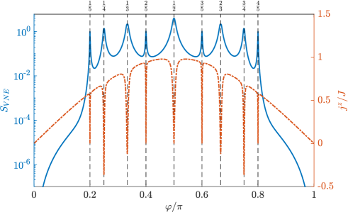
Figure 7: Von Neumann entropy of the NESS (solid blue line, left vertical scale) and steady-state magnetization current (dot-dashed red line, right vertical scale) as a function of the twisting angle $\varphi$. System parameters: $N=6$, $\Delta=\cos\varphi$, $\theta=\pi/2$, $\Gamma=500$. There are $9$ singular points characterized by peaks of $S_{VNE}$ and nadirs of $j^{z}$, where the convergence of the NESS to a pure spin-helix state fails. These points coincide with those predicted theoretically, see Eq. (62). Note the symmetry around $\varphi=\pi/2$.

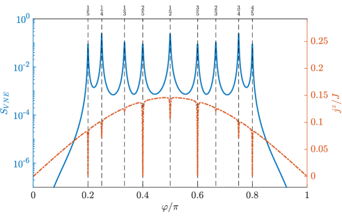
Figure 8: As in Fig. 7 but for $\theta=\pi/8$.

4.3 Source of $\Gamma_{\mathrm{ch}}$ singularities

All points of divergence of $\Gamma_{\mathrm{ch}}$ must be either due to divergence of $K^{-1}$, entering Eq. (53) directly, or the divergence of $\Lambda$ entering the expression (53) through the terms $Q_{\alpha,k}=\left\langle\alpha\right|[\Lambda h^{01},h^{k0}\left|0\right\rangle$, or both [2]. By using Mathematica we checked that each of the points (60) correspond to a divergence of either $K^{-1}$ or the $Q_{\alpha,k}(\Lambda)$ terms. The partition of the singularities of $\Gamma_{\mathrm{ch}}$ between $K^{-1}$ and $\Lambda$ depends quite crucially on the value of the polar angle $\theta$.

For $\theta\neq\pi/2$, we have $\det K\neq 0$ for any $\varphi$ and any $N$, therefore $K^{-1}$ always exists and all the points of divergence of $\Gamma_{\mathrm{ch}}$ are due to divergencies of the terms $Q_{\alpha,k}(\Lambda)$.

For $\theta=\pi/2$, $K^{-1}$ is singular at the isolated points $\varphi^{**}_{j}\in\Omega^{(K)}_{N}\subset\Omega^{*}_{N}$, where

$$\Omega^{(K)}_{N}=\left\{\varphi^{**}_{j}:\leavevmode\nobreak\ \varphi^{**}_{j}2k=\pi d,\leavevmode\nobreak\ k=1,2,\dots,\left\lfloor\frac{N-1}{2}\right\rfloor,\leavevmode\nobreak\ d=1,2,\dots,2k-1\right\}.$$ (67)

In this set, as in $\Omega^{*}_{N}$, pairs $d,k$ with the same ratio $d/(2k)$ are counted only once. The terms $Q_{\alpha,k}(\Lambda)$ diverge at the points of the complementary subset

$$\Omega^{(\Lambda)}_{N}=\Omega^{*}_{N}\setminus\Omega^{(K)}_{N}.$$ (68)

For example, in the case $N=6$ we have

$$\Omega^{(K)}_{6}=\left\{\frac{\pi}{2},\frac{\pi}{4},\frac{3\pi}{4}\right\},$$ (69)

$$\Omega^{(\Lambda)}_{6}=\left\{\frac{\pi}{3},\frac{\pi}{5},\frac{2\pi}{3},\frac{2\pi}{5},\frac{3\pi}{5},\frac{4\pi}{5}\right\}.$$ (70)

In Fig. 9 we show the minimum modulus of the eigenvalues of of the matrix $K$ as a function of the twisting angle $\varphi$ for $N=6$ and $\theta=\pi/2$. Zeros are obtained exactly at the points of the set (69).

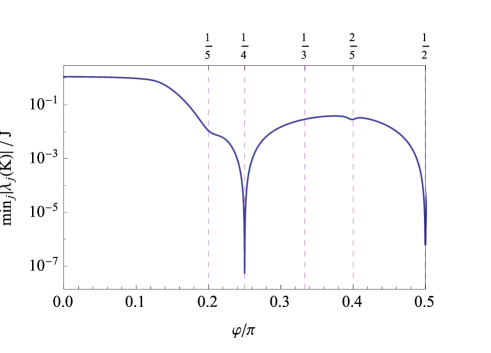
Figure 9: Minimum modulus of the eigenvalues of of the matrix $K$ as a function of the twisting angle $\varphi$ for $N=6$. The plot is symmetric with respect to $\varphi=\pi/2$ and $\varphi=0$. Parameters: $\theta=\pi/2$, $\Delta=\cos\varphi$.

The number of points in $\Omega^{(\Lambda)}_{N}$ is smaller than the number of points where $\Lambda$, tout court, has a divergence, namely, the points of degeneracy of $h^{00}$. This is easily understood if, instead of directly studing the divergences of the terms $Q_{\alpha,k}(\Lambda)$, we proceed as follows. A divergence of $\Gamma_{\mathrm{ch}}$ governed by the $\Lambda$ matrix stems from an inconsistency of the linear system of equations for the coefficients $M^{(1)}_{\alpha 0}$ arising in the first order expansion of the NESS in powers of $1/\Gamma$ [2]. In the basis in which $h^{00}$ is diagonal, this system has the form, see Eq. (A24) of [2],

$$(\lambda_{\alpha}-\lambda_{0})M^{(1)}_{\alpha 0}=2i\kappa\left\langle\alpha\right|h^{01}\left|0\right\rangle,\qquad\alpha=1,2,\dots,d_{1}-1.$$ (71)

Since $\kappa\neq 0$, the quantity $M^{(1)}_{\alpha 0}$ diverges if two conditions are simultaneously satisfied: (a) the eigenvalue $\lambda_{0}$ of $h^{00}$ is degenerate, i.e., $\lambda_{\alpha}-\lambda_{0}=0$ for some $\alpha=1,2,\dots,d_{1}-1$, and (b) for the corresponding $\alpha$ it results $\left\langle\alpha\right|h^{01}\left|0\right\rangle\neq 0$. Note that the sole degeneracy of $\lambda_{0}$ may not lead to a divergence of $\Gamma_{\mathrm{ch}}$.

Inspecting, for various finite $N$, the angles $\varphi$ where both (a) and (b) conditions are satisfied, we recover the subset $\Omega^{(\Lambda)}$ given by Eq. (68). The case $N=6$ with $\theta=\pi/2$ is shown in Fig. 10. Conditions (a) and (b) simultaneously hold at the points $\varphi/\pi=1/5,1/3,2/5$ as well as in the symmetric points $\varphi/\pi=3/5,2/3,4/5$ not shown in the plot.

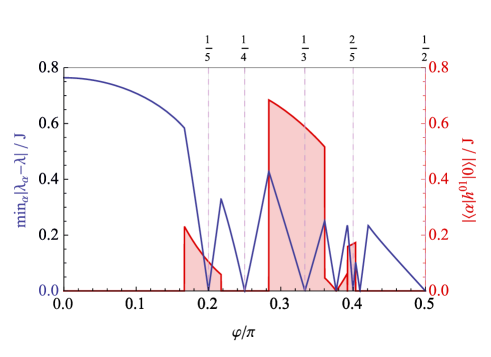
Figure 10: Gap of the $h^{00}$ spectrum (solid blue line, left vertical scale) and corresponding matrix element $\left\langle\alpha\right|h^{01}\left|0\right\rangle$ (dashed red line with filling to the horizontal axis, right vertical scale) as a function of the twisting angle $\varphi$ for $N=6$. Note that the gap vanishes and simultaneously $\left\langle\alpha\right|h^{01}\left|0\right\rangle\neq 0$ only at points $\varphi/\pi=1/5,1/3,2/5$. The plot is symmetric with respect to $\varphi=\pi/2$ and $\varphi=0$. Parameters: $\theta=\pi/2$, $\Delta=\cos\varphi$.

We conclude that the NESS reached in the Zeno limit becomes pure for all $\varphi$, except at the singular points of the set (60), where two or more spins in the target spin-helix configuration become collinear. In Fig. 11 we plot $\Gamma_{\mathrm{ch}}(\varphi)$ evaluated according to Eq. (53). The characteristic dissipation shows divergences exactly at the points predicted by (60). Note that in the thermodynamic limit $N\rightarrow\infty$ the number of divergencies grows quadratically with the system size.

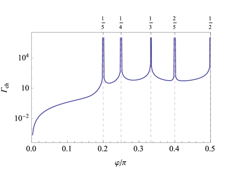
Figure 11: Characteristic dissipation $\Gamma_{\mathrm{ch}}$, computed according to Eq. (53), as a function of the twisting angle $\varphi$ for $N=6$. The plot is symmetric with respect to $\varphi=\pi/2$ and $\varphi=0$. Parameters: $\theta=\pi/2$, $\Delta=\cos\varphi$.

5 Experimental scenarios

Finally, we comment on two hypothetical experimental scenarios. Using single atom techniques [22], it should be possible to realize systems with a fixed number $N$ of spins $1/2$ coupled via Heisenberg exchange interaction, and to manipulate either the total twisting angle $\Phi$ (scenario A), or the anisotropy $\Delta$ (scenario B). For both cases, we assume that the dissipative strength $\Gamma$ can also be controlled. Note that quantum Zeno dynamics [23] is well within reach of contemporary experimental setups [24].

5.1 Scenario A. Fixed anisotropy $|\Delta|<1$, varying boundary twist $\Phi$

It is clear from the previous discussion that an interesting case occurs if the anisotropy $\Delta$ obeys $-1<\Delta<1$ and $\Delta\neq 0$. For a quantum chain, the regime $-1<\Delta<1$ is referred to as critical, or, an easy-plane regime, while the condition $\Delta\neq 0$ rules out the so-called noninteracting free-fermion case. The latter case corresponds to $\varphi=\pi/2$ and does not converge to a pure NESS for any $N$, see Eq. (66). Measuring any one of the NESS properties (a)-(c) discussed in Sec. 1, for different total boundary twisting angles $\Phi$, we will find a resonance-like behaviour in correspondence of the existence of a spin-helix pure NESS. This will happen at the value $\Phi=\Phi_{0}$ given by

$$\Phi_{0}=(N-1)\arccos\Delta.$$ (72)

The value of the characteristic dissipation above which the above resonance will be measured, can be computed analytically using Eq. (53). We have seen that the characteristic value $\Gamma_{\mathrm{ch}}$ becomes large in proximity of the singular points $\varphi^{*}_{j}$, where a divergence of $\Gamma_{\mathrm{ch}}$ takes place, see Eq. (60). The larger is the size of the system, the smaller is the distance between two consecutive singular points $\varphi^{*}_{j}$. Therefore, we expect $\Gamma_{\mathrm{ch}}(\Delta)$, with $\Delta$ corresponding to some generic irrational value of $\varphi=\arccos\Delta$, to increase with the system size $N$, and to diverge in the thermodynamic limit.

5.2 Scenario B. Fixed boundary twist $\Phi$, varying anisotropy $|\Delta|<1$

This scenario is more spectacular then the previous one. For every generic fixed twisting angle $\Phi$, such that $\Phi/\pi$ is an irrational, there will be $N-1$ resonance values of the anisotropy, corresponding to the formation of spin-helix states in the Zeno limit. These resonance values are given by $\Delta(m)=\cos((\Phi+2\pi m)/(N-1))$, $m=0,1,\dots,N-2$. The characteristic dissipation, above which the phenomenon can be measured, will depend on $m$ and on the closeness of the respective $\varphi=\arccos\Delta(m)$ to the nearest singular points $\varphi^{*}_{j}$ of Eq. (60). By increasing the size of the system we will have two competing effects. The number of resonances will grow linearly with the size $N$, but the majority of the spin-helix states will become more difficult to measure due to the overall growth of $\Gamma_{\mathrm{ch}}$. Note, however, that spin-helix states with the effective smallest winding numbers, namely, $m=0$ and $m=N-2$, become more accessible as the system size grows. In fact, we have observed in [15] that, for these winding numbers, $\Gamma_{\mathrm{ch}}(\epsilon)$, the characteristic dissipation at a chosen purity $\epsilon$ of the NESS, decreases by increasing $N$.

6 Conclusions

We have shown that a boundary-driven Heisenberg spin chain in the critical regime $|\Delta|<1$ exhibits, for large dissipation strength, a set of structural transitions in its nonequilibrium steady state between states with spatially smooth magnetization profile and spin-helix structures, where the local magnetization significantly changes from one site to another. Each spin-helix structure can be understood as a single generalized discrete Fourier harmonic, compatible with the boundary conditions imposed by the dissipation. Varying the anisotropy inside the critical easy-plane phase, $-1<\Delta<1$, and keeping sufficiently large dissipation strength, i.e., suppressing the boundary fluctuations, a complete set of these generalized discrete Fourier harmonics can be generated, one by one.

Note that with the help of spin-helix states (8) one can prepare a single spin in an arbitrary pure state, regardless of the length of the chain and the position of the spin, for any value of the anisotropy. This requires manipulating boundary dissipation at the ends of the chain. For isotropic spin exchange an arbitrary single spin state at a distance can be generated with just one boundary dissipator [25]. From the quantum transport point of view, existence of spin-helix states allows to reach ballistic current in a situation where typical current is diffusive or subdiffusive.

Interestingly, a structural transition to a spin-helix state fails, whenever two or more spins in the helix become collinear. Such a situation takes place when the twisting angle governing the helix is a rational number of $\pi$ and the spin chain is sufficiently long. At a deeper level, these breakups of convergence of the NESS to a pure state are related to divergences of the characteristic dissipation, a threshold value of the dissipation, above which the structural transitions can be observed. We have provided an explicit formula for the characteristic dissipation and a detailed classification of its divergences.

The method we propose can be straightforwardly generalized, and can be tested on other systems, e.g. on spin chains with higher spins, see [19]. It would be interesting to see if spin-helix–like structures can be realized in $1D$ arrays of magnetic atoms  [22].

Appendix A Dependence of $\Gamma_{\mathrm{ch}}$ on the polar angle $\theta$. Solvable case $N=3$

It is instructive to consider the simplest yet nontrivial chain with $N=3$ spins. In this case, the Hilbert spaces $\mathcal{H}_{0}$ and $\mathcal{H}_{1}$ have dimensions $d_{0}=2^{2}$ and $d_{1}=2^{1}$, respectively. The matrix $K$ is, therefore, a scalar and, using Eqs. (38), (54), (35), and (53), we find

$$K=-2\left(2\cos(2\varphi)\sin^{2}(\theta)+\cos(2\theta)+3\right).$$ (73)

Note that $K\leq 0$ for all $\theta,\ \varphi$ and $K=0$ only for $\theta=\pi/2,\ \varphi=\pi/2$. For $\Gamma_{\mathrm{ch}}$ we obtain the remarkably simple expression

$$\Gamma_{\mathrm{ch}}^{2}=8\sin^{4}(\theta)\sin^{2}(\varphi)\tan^{2}(\varphi).$$ (74)

We conclude that for $N=3$ the dependence of $\Gamma_{\mathrm{ch}}$ on $\theta$ is described by a multiplicative factor $\sin^{2}(\theta)$, which reaches its maximum at $\theta=\pi/2$.

For $N>3$, the $\theta$-dependence of $\Gamma_{\mathrm{ch}}$ is no longer multiplicative, however, it has the form

$$\frac{\Gamma_{\mathrm{ch}}(N,\varphi,\theta)}{\Gamma_{\mathrm{ch}}(N,\varphi,\pi/2)} =C_{N}(\varphi,\theta),$$ (75)

$$C_{N}(\varphi,\theta) =C_{N}(\varphi,\pi-\theta),$$ (76)

$$C_{N}(\varphi,\theta) \leq 1.$$ (77)

We have seen that $C_{3}(\varphi,\theta)=\sin^{2}(\theta)$, independent of $\varphi$. For $N>3$, the function $C_{N}(\varphi,\theta)$ at fixed $\varphi$ is always a symmetric function, $C_{N}(\varphi,\theta)=C_{N}(\varphi,\pi-\theta)$, which has an extremum at $\theta=\pi/2$. For most values of $\varphi$, $C_{N}(\varphi,\theta)$ has, as a function of $\theta$, an absolute maximum at $\theta=\pi/2$, see Fig. 12. For small $\theta\ll 1$, $C_{N}(\varphi,\theta)$ decreases as $\theta^{2}$, making the respective dissipative pure state (8) easier to reach (given purity attained at smaller dissipative strengths). This is in accordance with physical intuition since for small $\theta$ the spin-helix state (8) corresponds to small deviations of the local magnetization vector from the $(0,0,1)$ direction, which are easier to sustain.

Figure 12: Function $C_{N}(\varphi,\theta)$ versus $\theta$ for $N=5$ and $\varphi=\pi/2+0.01,2\pi/7,\pi/5,\pi/100$ (solid curves from bottom to top). The dashed gray line, shown for comparison, is $C_{3}(\varphi,\theta)=\sin^{2}\theta$.

References

References

- [1]
- [2] Popkov V, Presilla C and Schmidt J 2017 Phys. Rev. A 95(5) 052131
- [3] Gaudin M 2014 The Bethe Wavefunction (Cambridge University Press)
- [4] V E Korepin V E, Izergin A G and Bogoliubov N M 1993 Quantum Inverse Scattering Method, Correlation Functions and Algebraic Bethe Ansatz (Cambridge University Press)
- [5] Žnidarič M 2011 Journal of Statistical Mechanics: Theory and Experiment 2011 P12008
- [6] Žnidarič M 2011 Phys. Rev. Lett. 106(22) 220601
- [7] Prosen T 2011 Phys. Rev. Lett. 107(13) 137201
- [8] Prosen T 2015 Journal of Physics A: Mathematical and Theoretical 48 373001
- [9] Breuer H P and Petruccione F 2002 The Theory of Open Quantum Systems (Oxford University Press)
- [10] Plenio M B and Knight P L 1998 Rev. Mod. Phys. 70(1) 101–144
- [11] Clark S R, Prior J, Hartmann M J, Jaksch D and Plenio M B 2010 New Journal of Physics 12 025005
- [12] Landi G T, Novais E, de Oliveira M J and Karevski D 2014 Phys. Rev. E 90(4) 042142
- [13] Karevski D, Popkov V and Schütz G M 2013 Phys. Rev. Lett. 110(4) 047201
- [14] Popkov V, Karevski D and Schütz G M 2013 Phys. Rev. E 88(6) 062118
- [15] Popkov V and Presilla C 2016 Phys. Rev. A 93(2) 022111
- [16] Bernevig B A, Orenstein J and Zhang S C 2006 Phys. Rev. Lett. 97(23) 236601
- [17] Koralek J D, Weber C P, Orenstein J, Bernevig B A, Zhang S C, Mack S and Awschalom D D 2009 Nature 458 610–613
- [18] Winkler R 2003 Spin-orbit Coupling Effects in Two-Dimensional Electron and Hole Systems (Springer Tracts in Modern Physics) (Springer)
- [19] Popkov V and Schütz G M 2017 Phys. Rev. E 95(4) 042128
- [20] Ingham A E 1990 The Distribution of Prime Numbers (Cambridge Mathematical Library) (Cambridge University Press)
- [21] Popkov V 2012 Journal of Statistical Mechanics: Theory and Experiment 2012 P12015
- [22] Toskovic R, van den Berg R, Spinelli A, Eliens I S, van den Toorn B, Bryant B, Caux J S and Otte A F 2016 Nat Phys 12 656–660 letter
- [23] Facchi P and Pascazio S 2008 Journal of Physics A: Mathematical and Theoretical 41 493001
- [24] Schäfer F, Herrera I, Cherukattil S, Lovecchio C, Cataliotti F S, Caruso F and Smerzi A 2014 Nat Commun 5 3194
- [25] Žnidarič M 2016 Phys. Rev. Lett. 116(3) 030403