Characterizing Directed and Undirected Networks via Multidimensional Walks with Jumps

Abstract

Estimating distributions of node characteristics (labels) such as number of connections or citizenship of users in a social network via edge and node sampling is a vital part of the study of complex networks. Due to its low cost, sampling via a random walk (RW) has been proposed as an attractive solution to this task. Most RW methods assume either that the network is undirected or that walkers can traverse edges regardless of their direction. Some RW methods have been designed for directed networks where edges coming into a node are not directly observable. In this work, we propose Directed Unbiased Frontier Sampling (DUFS), a sampling method based on a large number of coordinated walkers, each starting from a node chosen uniformly at random. It is applicable to directed networks with invisible incoming edges because it constructs, in real-time, an undirected graph consistent with the walkers trajectories, and due to the use of random jumps which prevent walkers from being trapped. DUFS generalizes previous RW methods and is suited for undirected networks and to directed networks regardless of in-edges visibility. We also propose an improved estimator of node label distributions that combines information from the initial walker locations with subsequent RW observations. We evaluate DUFS, compare it to other RW methods, investigate the impact of its parameters on estimation accuracy and provide practical guidelines for choosing them. In estimating out-degree distributions, DUFS yields significantly better estimates of the head of the distribution than other methods, while matching or exceeding estimation accuracy of the tail. Last, we show that DUFS outperforms uniform node sampling when estimating distributions of node labels of the top 10% largest degree nodes, even when sampling a node uniformly has the same cost as RW steps.

Fabricio Murai, Bruno Ribeiro, Don Towsley and Pinghui Wang, 2017. Characterizing Directed and Undirected Networks via Multidimensional Walks with Jumps.

This work is supported by the Army Research Laboratory under Cooperative Agreement Number W911NF-09-2-0053 and the CNPq, National Council for Scientific and Technological Development - Brazil.

Author’s addresses: F. Murai, Universidade Federal de Minas Gerais; B. Ribeiro, Purdue University; D. Towsley, College of Information and Computer Sciences, University of Massachusetts Amherst; Pinghui Wang, Xi’an Jiaotong University.

1 Introduction

A number of studies [Boccaletti et al. (2006), Eagle et al. (2009), Leskovec and Faloutsos (2006), Leskovec et al. (2008), Mislove et al. (2007), Ribeiro et al. (2010), Rasti et al. (2009), Volz and Heckathorn (2008), Gjoka et al. (2010), Kurant et al. (2011b), Chiericetti et al. (2016)] are dedicated to the characterization of complex networks. Examples of networks of interest include the Internet, the Web, social, business, and biological networks. Characterizing a network consists of computing or estimating a set of statistics that describe the network. In this work we model a network as a directed or undirected graph with labeled vertices. A label can be, for instance, the degree of a node or, in a social network setting, someone’s hometown. Label statistics (e.g., average, distribution) are often used to characterize a network.

Characterizing a network with respect to its labels requires querying vertices and/or edges; associated with each query is a resource cost (time, bandwidth, money). For example, information about web pages must be obtained by querying web servers subject to a maximum query rate. Characterizing a large network by querying the entire network is often too costly. Even if the network is stored on disk it may constitute several terabytes of data. As a result, researchers have turned their attention to the characterization of networks based on incomplete (sampled) data.

Simple strategies such as uniform node and uniform edge sampling possess desirable statistical properties: the former yields unbiased samples of the population and the bias introduced by the latter is easily removed. However, these strategies are often rendered unfeasible because they require either a directory containing the list of all node (edge) ids, or an API that allows uniform sampling from the node (edge) space. Even when the space of possible node (edge) ids is known, its occupancy is usually so low that querying randomly generated ids is expensive. An alternate, cheaper, way to sample a network is via a random walk (RW). A RW samples a network by moving a particle (walker) from a node to a neighboring node. It is applicable to any network where one can query the edges connected to a given node. Furthermore, RWs share some of the desirable properties of uniform edge sampling (i.e., easy bias removal, accurate estimation of characteristics such as the tail of the degree distribution).

On one hand, a great deal of research has focused on the design of sampling methods for undirected networks using RWs [Heckathorn (1997), Rasti et al. (2009)]. Ribeiro and Towsley proposed Frontier Sampling (FS), a multidimensional random walk that uses $n$ coupled random walkers. This method yields more accurate estimates than the standard RW and also outperforms the use of $n$ independent walkers. In the presence of disconnected or loosely connected components, FS is even better suited than the standard RW and independent RWs to sample the tail of the degree distribution of the graph. On the other hand, few works have focused on the development of tools for characterizing directed networks in the wild. A network is said to be directed when edges are not necessarily reciprocated. Characterizing directed networks through crawling becomes especially challenging when only outgoing edges from a node are visible (incoming edges are hidden): unless all vertices have a directed path to all other vertices, a walker will eventually be restricted to a (strongly connected) component of the graph. Furthermore, a standard RW incurs a bias that can only be removed by conditioning on the entire graph structure. [Ribeiro et al. (2012)] addressed these issues by proposing Directed Unbiased Random Walk (DURW), a sampling technique that builds a virtual undirected graph on-the-fly and performs degree-proportional jumps to obtain asymptotically unbiased estimates of the distribution of node labels on a directed graph.

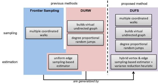
Figure 1: Proposed method (DUFS) generalizes Frontier Sampling and DURW.

In this work, we propose Directed Unbiased Frontier Sampling (DUFS), a method that generalizes the FS and the DURW algorithms (see Figure 1). Building on ideas in [Ribeiro et al. (2012)], we extend FS to allow the characterization of networks regardless of whether they are undirected, directed with observable incoming edges, or directed with unobservable incoming edges. From another perspective, we adapt DURW to use multiple coordinated walkers. DUFS matches or exceeds the accuracy of FS and DURW, as illustrated in Figure 2. Method parameters ($w$ and $b$), simulation setup, datasets and the error metric – NRMSE (normalized root mean square error) – are described in Section 5.1.

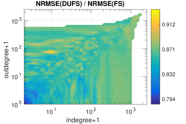
(a) soc-Slashdot0902

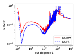
(b) livejournal-links

Figure 2: Comparison between proposed method (DUFS) and previous state-of-the-art respectively for visible and for invisible incoming edges scenarios; (a) NRMSE ratios between DUFS $(w=0.1,b=10)$ and FS $(b=10)$ of the estimated joint in- and out-degree distribution on the soc-Slashdot0902 dataset; (b) NRMSEs associated with DUFS and DURW of the estimated out-degree distribution on the livejournal-links dataset.

Contributions

Our main contributions are as follows:

1. Directed Unbiased Frontier Sampling (DUFS): we propose a new algorithm based on multiple coordinated random walks that extends Frontier Sampling (FS) to directed networks. DUFS extends DURW to multiple random walks.

2. A more accurate estimator for node label distribution: when the number of walkers is a large fraction of the number of random walk steps (e.g., 10%), a considerable amount of information is thrown out by not accounting for the walkers initial locations as observations. We introduce a new estimator that combines these observations with those made during the walks to produce better estimates.

3. Practical recommendations: we investigate the impact of the number of walkers and the probability of jumping to an uniformly chosen node (controlled via a parameter called random jump weight) on DUFS estimation error, given a fixed budget. By increasing the number of walkers the sequence of sampled edges approaches the uniform distribution faster, but this also increases the fraction of the budget spent to place the walkers in their initial locations. Moreover, increasing the random jump weight favors sampling node labels with large probability masses, which translates into more accurate estimates for these labels, but worse estimates for those in the tail. We study these trade-offs through simulation and propose guidelines for choosing DUFS parameters.

4. Comprehensive evaluation: we compare DUFS to other random walk-based methods applied to directed networks w.r.t. estimation errors, both when incoming edges are directly observable and when they are not. In the first scenario, in addition to some graph properties evaluated in previous works, we evaluate DUFS performance on estimating joint in- and out-degree distributions, and on estimating distribution of group memberships among the 10% largest degree nodes.

5. Theoretical analysis: we derive expressions for the normalized mean squared error associated with uniform node and uniform edge sampling on power law networks and show that in both cases error behaves asymptotically as a power law function of the observed degree. This helps explain our evaluation results.

Outline

Definitions are presented in Section 2. In Section 3, we review FS and DURW methods. In Section 4, we propose Directed Unbiased Frontier Sampling (DUFS) (along with some estimators), which generalizes previous methods. We investigate the impact of DUFS parameters on estimation accuracy of degree distributions and node label distributions respectively in Sections 5 and 6, providing practical guidelines on how to set them. A comparison to other random walk techniques is also provided. Section 7 discusses the performance of DUFS when the uniform node sampling mechanism is faulty. We present some related work and present our conclusions in Sections 8 and 9, respectively.

2 Terminology Setting

In what follows we present terminology used throughout the paper. We also present two scenarios considered in our work. Let $G_{d}=(V,E_{d})$ be a labeled directed graph representing the network graph, where $V$ is a set of vertices and $E_{d}$ is a set of ordered pairs of vertices $(u,v)$ representing a connection from $u$ to $v$ (a.k.a. edges). We refer to an edge $(u,v)$ as an in-edge with respect to $v$ and an out-edge with respect to $u$. The in-degree and out-degree of a node $u$ in $G_{d}$ are the number of distinct edges respectively into and out of $u$. We assume that each node in $G_{d}$ has at least one edge (either an in-edge or an out-edge). Some networks can be modeled as undirected graphs. In this case, $G_{d}$ is a symmetric directed graph, i.e., $(u,v)\in E_{d}$ iff $(v,u)\in E_{d}$.

Let $\mathcal{L}_{v}$ and $\mathcal{L}_{e}$ be finite (possibly empty) sets of node labels and edge labels, respectively. Each edge $(u,v)\in E_{d}$ is associated with a set of labels $\mathcal{L}_{e}(u,v)\subseteq\mathcal{L}_{e}$. For instance, one label $\ell\in\mathcal{L}_{e}(u,v)$ could be the nature of the relationship between two individuals (e.g., family, work, school) in a social network represented by nodes $u$ and $v$. Similarly, we can associate a set of labels to each node, $\mathcal{L}_{v}(v)\subseteq\mathcal{L}_{v},\,\forall v\in V$.

Input scenarios

When performing a random walk, we assume that a walker retrieves the out-edges of node where it resides by performing a query (e.g., followers list on Twitter) and that vertices are distinguishable. We define two scenarios depending on whether the walker can also retrieve in-edges.

In the first scenario, both out- and in-edges can be retrieved and it is possible to move the walker over any edge regardless of the edge direction (if the edge is $(u,v)\in E_{d}$ a walker can move from $u$ to $v$ and vice versa). In this case, the walker can be seen as moving over $G=(V,E)$, an undirected version of $G_{d}$, i.e., $E=\{(u,v):(u,v)\in E_{d}\lor(v,u)\in E_{d}\}$. Define $\deg(v)=|\{(u,v):(u,v)\in E\}|$. Let $\mbox{{vol}}(S)=\sum_{\forall v\in S}\deg(v),\,\forall S\subseteq V$, denote the volume of the set of vertices in $S\subseteq V$.

In the second scenario, only out-edges are directly observable and we can build on-the-fly an undirected graph $G_{u}$ based on the out-edges that have been sampled. Note that $G_{u}$ is not an undirected version of $G_{d}$ as some of the in-edges of a node may not have been observed. By moving the walker over $G_{u}$ – possibly traversing edges in $G_{d}$ in the opposite direction – we can compute its stationary behavior and thus, remove any bias by accounting for the probability that each observation appears in the sample.

While this has been mostly overlooked by other works, we emphasize that, in either scenario, it is useful to keep track of some variant of the observed graph during the sampling process. Storing information about visited nodes in memory saves resources that would be consumed to query those nodes in subsequent visits – i.e., revisiting a node has no cost. The specific variant of the observed graph to be stored will be described in the context of two random walk-based methods in the following section.

3 Background

The method proposed in this paper generalizes two representative random-walk based methods designed for each of the respective scenarios described in Section 2. Therefore, we dedicate this section to briefly reviewing these methods. First, we describe the Frontier Sampling algorithm proposed in [Ribeiro and Towsley (2010)], an $n$-dimensional random walk that benefits from starting its walkers at uniformly sampled vertices. This technique can be applied to undirected graphs and to directed graphs provided that edges coming into a node are observable. Then, we describe the Directed Unbiased Random Walk algorithm proposed in [Ribeiro et al. (2012)], that adapts a single random walk to a directed graph when incoming edges are not directly observable. The goal of these methods is to obtain samples from a graph, which are then used to infer graph characteristics via an estimator. An estimator is a function that takes a sequence of observations (sampled data) as input and outputs an estimate of an unknown population parameter (graph characteristic).

3.1 Frontier Sampling: a multidimensional random walk for undirected networks

In essence, Frontier Sampling (FS) is a random walk-based algorithm for sampling and estimating characteristics of an undirected graph. FS performs $n$ coordinated random walks on the graph. One of the advantages of using multiple walkers is that they can cover multiple connected components (when they exist), while a single walker is restricted to one component in the absence of a random jump or restart mechanism. By coordinating multiple random walkers, FS is able to sample edges uniformly at random in steady state regardless of how the walkers are initially placed.

Input : sampling budget $B$, budget per walker $b$, cost of uniform node sampling $c$

1 $n\leftarrow B/(c+b)$ ;

2 Initialize $L=(v_{1},\dots,v_{N})$ with $n$ randomly chosen vertices (uniformly);

3 $i\leftarrow N\times c$ {$i$ is the used portion of the budget};

4 while $i<B$ do

5       Select $u\in L$ with probability $\deg(u)/\sum_{\forall v\in L}\deg(v)$ ;

6       Select an edge $(u,v)$, uniformly at random;

7       Replace $u$ by $v$ in $L$ and add $(u,v)$ to sequence of sampled edges;

8       $i\leftarrow i+1$ {can be skipped if node was previously sampled} ;

9      

10 end while

ALGORITHM 1 Frontier Sampling (FS)

Algorithm 1 describes FS. There are three parameters: the sampling budget $B$, the initial cost of placing a walker $c\geq 1$ and the average number of nodes $b$ sampled by a walker. The initial walker locations are chosen uniformly at random over the node set (line 2). Note that the number of walkers is taken to be $n=B/(c+b)$, that the cost of a random walk step is one (except for previously sampled nodes) and that the cost of initially placing a walker, $c$, can be greater than one because uniform node sampling is often expensive. FS keeps a list $L$ of $n$ vertices representing the locations of the $n$ walkers. At each step, a walker is chosen from $L$ in proportion to the degree of the node where it is currently located (line 5). The walker then moves from $u$ to an adjacent node $v$ (lines 6 and 7).

Frontier sampling is equivalent to the sampling process of a single random walker over the $n$-th Cartesian power of $G$. For this reason, Frontier Sampling can be thought of as an $n$-dimensional random walk (see [Ribeiro and Towsley (2010), Lemma 5.1]).

Using FS samples to estimate node label distributions is simple when the input corresponds to the first scenario described in Section 2. The probability of sampling a given node is proportional to its undirected degree in $G$. Hence, each sample must be weighted inversely proportional to the respective node’s undirected degree. Storing the undirected version of the observed graph along with labels associated with sampled nodes allows the sampler to avoid having to pay the cost of revisiting a node.

Conversely, when incoming edges are not observed, Frontier Sampling can still be adapted to remove bias. We present this method in Section 4.

3.2 Directed Unbiased Random Walk: a random walk adapted for directed networks with unobservable in-edges

The presence of hidden incoming edges but observable outgoing edges makes characterizing large directed graphs through crawling challenging. Edge $(u,v)$ is a hidden incoming edge of node $v$ if $(u,v)$ can only be observed from node $u$. For instance, in Wikipedia we cannot observe the edge (“Columbia Records”, “Thomas Edison”) from Thomas Edison’s wiki entry (but this edge is observable if we access the Columbia Records’s wiki entry).

These hidden incoming edges make it impossible to remove any bias incurred by walking on the observed graph, unless we crawl the entire graph. Moreover, there may not even be a directed path from a given node to all other nodes. Graphs with hidden outgoing edges but observable incoming edges exhibit essentially the same problem. In [Ribeiro et al. (2012)], we proposed the Directed Unbiased Random Walk (DURW) algorithm, which obtains asymptotically unbiased estimates of node label densities on a directed graph with unobservable incoming edges. Our random walk algorithm follows two main principles to achieve unbiased samples and reduce variance:

• Backward edge traversals: in real-time we construct an undirected graph $G_{u}$ using nodes that are sampled by the walker on the directed graph $G_{d}$. The role of the undirected graph is to guarantee that, at the end of the sampling process, we can approximate the probability of sampling a node, even though in-edges are not observed. The random walk proceeds in such a way that its trajectory on $G_{d}$ is consistent with that of a random walk on $G_{u}$. The walker is allowed to traverse some of the edges in $G_{d}$ in a reverse direction. However, we prevent some of the observed edges to be traversed in the reverse direction by not including them in $G_{u}$. More precisely, once a node $z$ is visited at the $i$-th step, no in-edges to $z$ observed at step $j>i$ (by visiting nodes $s$ such that $(s,z)\in E_{d}$) are added to $G_{u}$. This is an important feature to reduce the random walk transient and thus, reduce estimation errors.

• Degree-proportional jumps: the walker makes a limited number of random jumps to guarantee that different parts of the directed graph are explored. In DURW, the probability of randomly jumping out of a node $v$, $\forall v\in V$, is $w/(w+\deg(v))$, $w>0$. The steady state probability of visiting a node $v$ on $G_{u}$ is $(w+\deg(v))/(\mbox{{vol}}(V)+w|V|)$. Similar to the cost of placing a FS walker through uniform node sampling, we assume that each random jump incurs cost $c\geq 1$.

The DURW algorithm

DURW is a random walk over a weighted undirected connected graph $G_{u}=(V,E_{u})$, which is built on-the-fly. We build an undirected graph using the underlying directed graph $G_{d}$ and the ability to perform random jumps. Let $G^{(i)}=(V,E^{(i)})$ denote the undirected graph constructed by DURW at step $i$, where $V$ is the node set and $E^{(i)}$ is the edge set. In what follows we describe the construction of $G^{(i)}$ in Algorithm 2, since this is one of the building blocks of the proposed algorithm, DUFS.

Input : sampling budget $B$, random jump weight $w$, cost of uniform node sampling $c$

1 Select $s\in V$ uniformly at random {$s=s_{1}$} ;

2 Initialize $\mathcal{S}=\{s\}$ and $E=\mathcal{E}(s)$ ;

3 $i\leftarrow c$ {$i$ is the used portion of the budget};

4 while $i<B$ do

5       $p\sim\textrm{Uniform}(0,1)$ ;

6       if $p\leq w/(w+\textrm{deg}(s))$ then

7             Select $s$ uniformly at random from $V$ {random jump} ;

8             $i\leftarrow i+c$ ;

9            

10      else

11             Select $s$ uniformly at random from $\{v:(s,v)\in E\}$ {random walk step} ;

12             $i\leftarrow i+1$ ;

13            

14       end if

15      if $s\notin\mathcal{S}$ then

16             $\mathcal{S}\leftarrow\mathcal{S}\cup\{s\}$ ;

17             $E\leftarrow E\cup\{(s,v)\in\mathcal{E}(s):v\not\in\mathcal{S}\}$

18       end if

19      

20 end while

ALGORITHM 2 Construction of undirected graph (common to DURW and DUFS)

Let $\mathcal{E}(v)$ denote the set of out-edges from a node $v$ in $G_{d}$. Let $\mathcal{S}^{(i)}=\{s_{1},\ldots,s_{i}\}$ be the set of nodes from $V$ sampled by the random walk up to step $i$, where $s_{j}$ denotes the node on which the walker resides at step $j$. Since $V$ is not known, we track $G^{(i)}$ using variables $\mathcal{S}=\mathcal{S}^{(i)}$ and $E=E^{(i)}$. The walker starts at node $s_{1}\in V$ (line 1). We initialize $G^{(1)}=(V,E^{(1)})$, where $E^{(1)}=\mathcal{E}(s_{1})$ (line 2). The next node, $s_{i+1}$, is selected uniformly at random from $V$ with probability $w/(w+\textrm{deg}(s_{i}))$ (lines 6 to 8), where $\textrm{deg}(s_{i})$ is the degree of $s_{i}$ in $G^{(i)}$. With probability $1-w/(w+\textrm{deg}(s_{i}))$, node $s_{i+1}$ is selected by performing a random walk step from $s_{i}$, i.e. by selecting a node adjacent to $s_{i}$ in $E^{(i)}$ uniformly at random (lines 9 to 12). When node $s_{i+1}$ is visited for the first time, it is necessary to set $\mathcal{S}^{(i+1)}$ to $\mathcal{S}^{(i)}\cup\{s_{i+1}\}$ and $E^{(i+1)}$ to $E^{(i)}\cup\{(s_{i},v)\in\mathcal{E}(s_{i}):v\not\in\mathcal{S}^{(i)}\}$ (lines 13 to 16). By restricting the set of new edges to $\{(s_{i},v)\in\mathcal{E}(s_{i}):v\not\in\mathcal{S}^{(i)}\}$ instead of all edges visible from $s_{i}$ (i.e., $\mathcal{E}(s_{i})$), we comply with the requirement that once a node $z$, $\forall z\in V$, is visited by the RW, no edge can be added to $G_{u}$ with $z$ as an endpoint.

In order to estimate node label distributions from DURW observations, we weight samples in proportion to the inverse probability that the corresponding vertices are visited by a random walk in $G_{u}$, in steady state. Storing labels and edges associated with nodes in $\mathcal{S}^{(i)}$ saves the cost of querying repeated nodes. Such savings could be reflected in Algorithm 2 by conditioning the increase in $i$ (lines 2 and 2) on $s\notin\mathcal{S}$.

4 Generalizing FS and DURW: a new method applicable regardless of in-edge visibility

This section is divided into two parts. In Section 4.1 we propose Directed Unbiased Frontier Sampling (DUFS), which generalizes FS to allow estimation on directed graphs with unobservable in-edges (second scenario described in Section 2). DUFS also generalizes DURW: the latter is a special case of DUFS where the number of walkers is one. Next, in Section 4.2, we describe two ways to estimate node label distributions using DUFS. The first uses only on the observations collected during the walks. The second estimator we leverages observations obtained from the initial walker locations in addition to observations obtained during the walks.

4.1 Directed Unbiased Frontier Sampling

Like FS, Directed Unbiased Frontier Sampling (DUFS) samples a network through $n$ coordinated walks. At each step, it selects a walker in proportion to the degree of the node where it currently resides. Similar to the Directed Unbiased Random Walk, it constructs an undirected graph in real-time that allows backward edge traversals. Denote by $G^{(i)}=(V,E^{(i)})$ the undirected graph constructed by DUFS at step $i$. DUFS does not include edges in $G^{(i)}$ that would cause walkers to have a view of the graph inconsistent with the view at a previous point in time. In other words, when node $u$ is visited for the first time at step $i$, $u$ is inserted in $G^{(i)}$ along with all edges $(u,v)\in E_{d}$ such that $v$ has not been sampled. Thus, the degree of $u$ is fixed in $G^{(j)}$, for all $j\geq i$. Alternatively, letting the degree of $u$ change at a given point would require us to discard the the entire sample up to that point, otherwise the resulting estimator would not be consistent. In fact, even that approach would not yield a consistent estimator for an infinite power law graph: node degrees would never stop changing.

It may seem that there is no need to include degree-proportional jumps to visit different graph components when a large number of walkers are initially spread throughout the graph (e.g., on nodes chosen uniformly). However, including degree-proportional jumps in DUFS is extremely beneficial because it prevents walkers from being trapped when initially located on vertices whose out-degree is zero or in components with no outgoing edges. More generally, it allows walkers to move from small volume to large volume components and, hence, obtain more samples among large degree nodes.

Algorithm 3 describes DUFS. In addition to FS’ three parameters, it takes a random jump weight $w$ as input. The number of walkers and their initial locations are chosen as in FS (lines 1-3). In the extreme case where $b=0$, DUFS degenerates to uniform node sampling. When the underlying graph is symmetric and the jump weight is $w=0$, it becomes FS. When in-edges are invisible and the number of walkers is 1, DUFS degenerates to DURW. We initialize $\mathcal{S}=L$ and $E^{(i)}=\cup_{s\in L}\mathcal{E}(s)$ (line 4). Unlike in FS, a walker is chosen from $L$ in proportion to the sum of the random jump weight $w$ and the degree of node where it is currently located based on $E^{(i)}$ (line 6). Similar to DURW, the next node is selected based on either a random jump or on following an edge (lines 7-14). Last, the undirected graph is updated (lines 15-18) and so is set $L$ (line 19).

Input : sampling budget $B$, budget per walker $b$, cost of uniform sampling $c$, jump weight $w$

1 $n\leftarrow B/(c+b)$ {$n$ is the number of walkers};

2 Initialize $L=\{v_{1},\dots,v_{N}\}$ with $n$ randomly chosen vertices (uniformly);

3 $i\leftarrow N\times c$ {$i$ is the used portion of the budget};

4 Initialize $\mathcal{S}=L$ and $E=\cup_{s\in L}\mathcal{E}(s)$ ;

5 while $i<B$ do

6       Select $v\in L$ with probability $(w+\deg(v))/(nw+\sum_{\forall v_{j}\in L}\deg(v_{j}))$ ;

7       Sample $p\sim\textrm{Uniform}(0,1)$;

8       if  $p<w/(w+\deg(v))$ then

9             Select a node $v\in V$ uniformly at random;

10             $i\leftarrow i+c$;

11            

12      else

13             Select an outgoing edge of $v$, $(v,v^{\prime})$, uniformly at random;

14             $i\leftarrow i+1$;

15            

16       end if

17      if $s\notin\mathcal{S}$ then

18             $\mathcal{S}\leftarrow\mathcal{S}\cup\{s\}$ ;

19             $E\leftarrow E\cup\{(s,v)\in\mathcal{E}(s):v\not\in\mathcal{S}\}$

20       end if

21      Replace $v$ by $v^{\prime}$ in $L$ and add $(v,v^{\prime})$ to sequence of sampled edges;

22      

23 end while

ALGORITHM 3 Directed Unbiased Frontier Sampling (DUFS)

4.2 Estimation

In this section we describe two estimators of node label distributions from samples obtained by DUFS. The first estimator is based on the observations obtained from edges traversed by the random walks. The second estimator combines these observations with those obtained from the walkers initial locations. When used with a variance reduction heuristic, the latter produces better estimates than the former. For a description of estimators of edge label distribution and other graph characteristics, please refer to [Ribeiro and Towsley (2010)].

4.2.1 Node Label Distribution: random edge-based estimator

Let $s_{i}$ denote the $i$-th node visited by DUFS, $i=1,\dots,t$, $t\leq B-Nc$. Let $\theta_{\ell}$ be the fraction of nodes in $V$ with label $\ell\in\mathcal{L}_{v}$. Let $\pi(v)$ be the steady state probability of sampling node $v$ in $G_{u}$, $\forall v\in V$. The node label distribution is estimated at step $t$ as

$$\hat{\theta}_{\ell}=\frac{1}{n}\sum_{i=1}^{t}\frac{\mathds{1}\{\ell\in\mathcal{L}_{v}(v)\}}{\hat{\pi}(s_{i})}\,,\qquad\ell\in\mathcal{L}_{v},\,t=1,\ldots,B-Nc,$$ (1)

where $\mathds{1}\{P\}$ takes value one if predicate $P$ is true and zero otherwise, and $\hat{\pi}(s_{i})$ is an estimate of $\pi(s_{i})$: $\hat{\pi}(s_{i})=(w+\deg(s_{i}))S$. Here $\deg(v)$ is the degree of $v$ in $G^{(\infty)}$ and

$$S=\frac{1}{t}\sum_{i=1}^{t}\frac{1}{w+\deg(s_{i})}\,.$$ (2)

The following theorem states that $\hat{\pi}(s_{i})$ is asymptotically unbiased.

Theorem 4.1.

$\hat{\pi}(s_{i})$ is an asymptotically unbiased estimator of $\pi(s_{i})$.

Proof 4.2.

To show that $\hat{\pi}(s_{i})$ is asymptotically unbiased, we first note that the limit $\lim_{t\to\infty}E^{(t)}=E^{(\infty)}$ exists, since after visiting all vertices we will never add any additional edges. We then invoke Theorem 4.1 of [Ribeiro and Towsley (2010)], yielding $\lim_{t\to\infty}S=|V|/(|E^{(\infty)}|+|V|w)$ almost surely. Thus, $\lim_{t\to\infty}\hat{\pi}(s_{i})={\pi}(s_{i})$ almost surely. Taking the expectation of (1) in the limit as $t\to\infty$ yields $E[\lim_{t\to\infty}\hat{\theta}_{\ell}]={\theta}_{\ell},$ which concludes our proof.

4.2.2 Node Label Distribution: leveraging information from walkers’ initial locations

The estimator presented in (1) does not make use of information associated with the initial set of nodes on which the walkers are placed. When the number of walkers is large this results in the loss of a considerable amount of statistical information. However, including these observations is challenging because subsequent observations from random walk steps are not independent of the initial observations. Moreover, the normalizing constant for the random walk observations is no longer given by (2), since degree distribution estimates also depend on the information contained in the node samples.

In this section, we derive a new estimator that circumvents these problems by approximating the likelihood of RW samples by that associated with random edge sampling. We call it the hybrid estimator because it combines observations from initial walker locations and random walks steps. The hybrid estimator significantly improves the estimation accuracy for labels associated with large probability masses.

Let us index the node labels $\mathcal{L}_{v}$ from $1$ to $W$, where $W=|\mathcal{L}_{v}|$. We refer to the sum $\deg(v)+w$ in DUFS as the random walk bias for node $v\in V$. To simplify the notation, we assume that each node has exactly one label and that random walk biases take on integer values in $[1,\ldots,Z]$, for some maximum value $Z$. Denote the node label distribution as ${\boldsymbol{\theta}}=(\theta_{1},\ldots,\theta_{W})$. Let $n_{i}$ denote the number of walkers starting on label $i$ nodes and $m_{i,j}$ the number of subsequent observations of label $i$ and bias $j$ nodes. The notation is summarized in Table 1.

Variable	Description
$n_{i}$	number of node samples with label $i$
$\theta_{i,j}$	fraction of nodes in $G^{(t)}$ with label $i$ and undirected degree $j$
$m_{i,j}$	number of edge samples with label $i$ and bias $j$
$m_{i}=\sum_{j}m_{i,j}$	total number of edge samples with label $i$
$N=\sum_{i}n_{i}$	total number of node samples
$M=\sum_{i}m_{i}$	total number of edge samples
$B=N+M$	total budget

Table 1: Notation used in hybrid estimator.

We approximate random walk samples in DUFS by uniform edge samples from $G_{u}$. Experience from previous studies shows us that this approximation works very well in practice. Hence, the likelihood function given samples $\mathbf{n}=\{n_{i}:i=1,\ldots,W\}$ and $\mathbf{m}=\{m_{i,j}:i=1,\ldots,W\textrm{ and }j=1,\ldots,Z\}$ is expressed as

$$L({\boldsymbol{\theta}}|\mathbf{n},\mathbf{m})=\frac{\prod_{i}\theta_{i}^{n_{i}}\prod_{k}(k\theta_{i,k})^{m_{i,k}}}{\left(\sum_{s,t}t\theta_{s,t}\right)^{M}}.$$ (3)

The maximum likelihood estimator $\theta^{\star}$ is the value of $\theta$ that maximizes (3) subject to $0\leq\theta_{i}\leq 1$ and $\sum_{i}\theta_{i}=1$. This defines a constrained non-convex optimization problem. However, we can convert this optimization problem into an unconstrained problem using the reparameterization $\theta_{i}=e^{\beta_{i}}/\sum_{k}e^{\beta_{k}}$ for $i=1,\ldots,W$. As shown in Appendix A, the partial derivatives of the resulting objective function are

$$\frac{\partial\mathcal{L}({\boldsymbol{\beta}}|\mathbf{n},\mathbf{m})}{\partial\beta_{i}}=n_{i}+m_{i}-\frac{Ne^{\beta_{i}}}{\sum_{j}e^{\beta_{j}}}-\frac{Me^{\beta_{i}}m_{i}/\mu_{i}}{\sum_{s}e^{\beta_{s}}m_{s}/\mu_{s}},\qquad i=1,\ldots,W,$$ (4)

where $m_{i}=\sum_{k}m_{i,k}$ and $\mu_{i}=\sum_{k}m_{i,k}/k$. Setting one of the variables to a constant (say, $\beta_{W}=1$) for identifiability and then using the gradient descent method to change the remaining variables according to (4) is guaranteed to converge provided that we make small enough steps. An interesting interpretation of (4) is obtained by setting the derivatives to zero and substituting back $\theta_{i}=e^{\beta_{i}}/\sum_{k}e^{\beta_{k}}$:

$$\theta_{i}^{\star}=(n_{i}+m_{i})\left(N+M\frac{m_{i}/\mu_{i}}{\sum_{s}\theta_{s}^{\star}m_{s}/\mu_{s}}\right)^{-1},\qquad i=1,\ldots,W.$$ (5)

According to (5), the estimated fraction of nodes with label $i$ is the total number of times label $i$ was observed (i.e., $n_{i}+m_{i}$) normalized by sum of (i) the number of random node samples and (ii) the number of random edge samples weighted by the probability of sampling label $i$ from one random edge sample. In the limit as $N$ and $M$ go to infinity, we can show that ${\boldsymbol{\theta}}^{\star}={\boldsymbol{\theta}}$ is a solution, but we cannot prove that it is unique or that ${\boldsymbol{\theta}}^{\star}$ converges to ${\boldsymbol{\theta}}$. Hence, we cannot prove that ${\boldsymbol{\theta}}^{\star}$ is asymptotically unbiased.

The system of non-linear equations determined by (5) cannot be solved directly, but can be tackled by Expectation Maximization (EM). In this case, the term $\sum_{s}\theta_{s}^{\star}m_{s}/\mu_{s}$ in the denominator is replaced by its expected value given $\theta_{i}$’s from the previous iteration. Based on the same idea, if we replace $\sum_{s}\theta_{s}^{\star}m_{s}/\mu_{s}$ with an edge sampled-based estimator $\hat{d}$ for the average degree in $G_{u}$, we obtain the following non-recursive variant of the hybrid estimator,

$$\hat{\theta}_{i}=(n_{i}+m_{i})\left(N+M\frac{m_{i}}{\mu_{i}\hat{d}}\right)^{-1},\qquad i=1,\ldots,W,$$ (6)

where $\hat{d}=M/(\sum_{i}\mu_{i})$. Theorem 1 below states the conditions under which $\hat{\theta}_{i}$ is asymptotically unbiased (see appendix for proof). In practice, we find no significant difference between $\theta_{i}^{\star}$ and $\hat{\theta}_{i}$, except when the number of walkers $N$ is very large and the jump weight $w$ is very small. For those cases, $\theta_{i}^{\star}$ tends to be slightly more accurate than $\hat{\theta}_{i}$ for small values of $i$, which in some applications may justify the additional computational cost of executing gradient descent or EM.

Theorem 1.

Let $N=\alpha B$ and $M=(1-\alpha)B$, for some $0<\alpha<1$. In the limit as $B\rightarrow\infty$, the estimator $\hat{\theta}_{i}$ is an unbiased estimator of $\theta_{i}$.

In the special case where the label is the undirected degree itself, we have $\mu_{i}=m_{i}/i$. Hence, eq. (6) reduces to

$$\bar{\theta}_{i}=\frac{n_{i}+m_{i}}{N+Mi/\hat{d}},$$ (7)

where $\hat{d}$ is the estimated average degree. When the average degree is known, we can show that $\bar{\theta}_{i}$ is unbiased and, moreover, the minimum variance unbiased estimator (MVUE) of $\theta_{i}$ (see appendix for proof).

When $n_{i}>0$ but $m_{i}=0$, the estimator in eq. (6) reduces to $\hat{\theta}_{i}=n_{i}/N$, which is essentially the MLE for uniform node sampling. It is well known that this estimator is not nearly as accurate as a random walk based estimator for large out-degree values with small probability mass. In some sense, the estimator $\hat{\theta}_{i}=n_{i}/N$ does not account for the fact that the number of random walk samples is zero. As a result, mass estimates for large out-degrees tend to have very large variance when no random walk samples are observed. Fortunately, we find that the following heuristic rule can drastically reduce the estimator variance in these cases.

Variance reduction rule

If no random edge samples are observed for out-degree $i$, we set the estimate $\hat{\theta}_{i}=0$. This implies that we ignore any random node samples seen of nodes that have out-degree $i$. While this clearly results in a biased estimate, as the budget per walker $b$ goes to infinity, the probability of invoking this rule goes to zero. Hence, it produces an asymptotically unbiased estimate. This rule can be interpreted as a combination of node-based and edge-based estimates in proportion to the reciprocals of their estimated variances. That is, when no random edge samples are observed for a given out-degree, the corresponding estimated variance is zero and hence, random node samples should be ignored. We note that the converse rule (i.e., set $\hat{\theta}_{i}=0$ if no random node samples were observed) would not perform well, as the probability of sampling large out-degrees with random node sampling is very small.

We simulate DUFS on several datasets and compare the results obtained with the hybrid estimator when the rule is used and when it is not. Simulation details, datasets and the error metric (normalized root mean square error) will be described in Section 5.1. Figure 3 shows representative results of the impact of the rule when estimating out-degree distributions using DUFS in conjunction with the hybrid estimator on two network datasets (averaged over 1000 runs). The results show that the rule consistently reduces estimation error in the distribution tail without affecting estimation quality for small values of $i$.

Figure 3: (visible in-edges) Effect of variance reduction rule on NRMSE, when $B=0.1|V|$ and $c=1$. Using information contained in random node samples can increase variance for large out-degree estimates. However, the proposed rule effectively controls for that effect without decreasing head estimates accuracy.

In-degree distribution: impossibility result

The fact that long random walks are often approximated by random edge sampling brings up the question of whether they can be used to estimate in-degree distributions when the in-degree is not observed directly. Under random edge sampling, the number of observed edges pointing to a node is binomially distributed and a maximum likelihood estimator can be derived for estimating the in-degree distribution. This problem is related to the set size distribution estimation problem, where elements are randomly sampled from a collection of non-overlapping sets and the goal is to recover the original set size distribution from samples. In addition to in-degree distribution in large graphs, this problem is related to the uncovering of TCP/IP flow size distributions on the Internet.

In [Murai et al. (2013)], we derive error bounds for the set size distribution estimation problem from an information-theoretic perspective. The recoverability of original set size distributions presents a sharp threshold with respect to the fraction of elements sampled from the sets. If this fraction lies below the threshold, typically half of the elements in power-law and heavier-than-exponential-tailed distributions, then the original set size distribution is unrecoverable (see [Murai et al. (2013), Theorem 2]).

5 Results on degree distribution estimation

Here we focus on the estimation of degree distributions on directed networks. This section is divided into four parts. In Section 5.1, we investigate the impact of DUFS parameters on estimation accuracy. We then compare DUFS against other random walk-based methods when both outgoing and incoming edges are visible in Section 5.2. In Section 5.3, we perform a similar comparison when only out-edges are visible. Last, in Section 5.4 we provide some analysis to explain the relationship observed between the NRMSE and the out-degree (in-degree) in the results. We will refer to the edge-based estimator defined in (1) as E-DUFS.

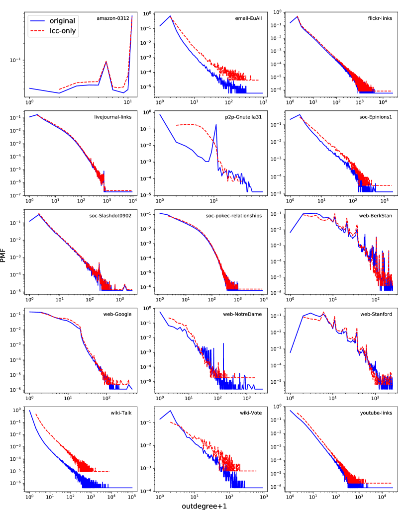
Figure 4: Out-degree probability mass function (p.m.f.) for each network and its largest strongly connected component (LCC). A large difference between these p.m.f.s suggests it is beneficial to use multiple walkers and/or random jumps.

The 15 directed network datasets in our evaluation were obtained from Stanford’s SNAP [Leskovec and Krevl (2014)]. These datasets describe the topology of a variety of social networks, communication networks, web graphs, one Internet peer-to-peer networks and one product co-purchasing networks. We found it informative to extract the largest strongly connected component of each directed network and to apply our methods to the resulting datasets – hereby referred to as LCC datasets – as well as to the original datasets. Figure 4 shows the out-degree probability mass function (p.m.f.) for each network, along with the out-degree p.m.f. for the corresponding LCC dataset. We opt to show the p.m.f. instead of the complementary cumulative distribution function (CCDF) because the estimation task in this work is defined in terms of the p.m.f.’s. Defining the estimation task in terms of the CCDF would give DUFS an unfair advantage, as we will explain in Section 5.2.

Simulations consist of sampling the network until a budget $B=0.1|V|$ (i.e., 10% of the number of vertices) is depleted. Note that budget is decremented when walkers are initially placed and each time one of them moves to a node and when they perform random jumps. We construct an undirected graph in the background throughout each simulation. As a result, we assume that the cost to revisit a node is zero, even if this visit occurs due to a random jump.

When both outgoing and incoming edges are observable, random walks disregard edge direction, and move as if the network is undirected. In this scenario, we focus either on the estimation of the marginal out- and in-degree distributions or the joint distribution. The methods we investigate here can be used to estimate other node label distributions. For instance, if the underlying network is undirected, we can estimate the (undirected) degree distribution or even non-topological properties, such as the distribution of user nationalities in a social network. In the light of the impossibility results described in the end of Section 4.2, we focus on out-degree distribution estimation when incoming edges are not directly observable.

Let ${\boldsymbol{\theta}}=\{\theta_{i}\}_{\forall i\in\mathcal{L}}$ denote the node label distribution, where $\theta_{\ell}$ is the fraction of vertices with label $\ell$. Denote by $\hat{\theta}_{\ell}$ the estimate for $\theta_{\ell}$. We use normalized root mean square error (NRMSE ) of $\hat{\theta}_{\ell}$ as the error metric, which is a normalized measure of the dispersion of the estimates, defined as

$$\mbox{{NRMSE}}(\ell)=\frac{\sqrt{E[(\hat{\theta_{\ell}}-\theta_{\ell})^{2}]}}{\theta_{\ell}}.$$ (8)

In the case of marginal in-degree (out-degree) distribution, we refer to in-degrees (out-degrees) smaller than the average as the head of the distribution. We refer to the largest 1% in- (out-degree) values as the tail of the distribution.

5.1 Impact of DUFS parameters and practical guidelines

To provide intuition on how random jump weight $w$ and budget per walker $b$ affect the accuracy of DUFS estimates, assume for now that we replace samples collected via random walks by uniform edge samples from the weighted undirected graph $G_{u}$. In this hypothetical scenario, the budget $B$ is used to collect $N\geq 1$ uniform node samples and $B-Nc$ uniform edge samples. Clearly, when the edge-based estimator defined in (1) is used, the most accurate node label distribution estimates are obtained by setting $N=1$, (i.e. $b=B-c$). Hence, we focus on the case where the hybrid-estimator defined in (5) is used. In particular, consider estimation of the out-degree distribution.

For a given value of $b$, the number of uniform node samples will be $B/(c+b)$. For each of the remaining $B-B/(c+b)$ samples, a vertex $v$ is sampled in proportion to $\deg(v)+w$, where $\deg(v)$ is the undirected degree of $v$ in $G_{u}$. The choice of $w$ and $b$ impose, individually, a trade-off between estimation accuracy of the head and of tail of the distribution. For a fixed value of $w$, smaller values of $b$ translate into better estimates of the head (and worse estimates of the tail) because we collect more (less) information about that region of the distribution from uniform node samples. For a fixed value of $b$, larger values of $w$ also translate into more (less) accurate estimates of the head (tail), because random jumps are more likely to move a node to low in- and out-degree nodes (as they tend to occur more frequently).

In what follows, we observe through simulations that despite the uniform edge sampling approximation, the previous intuition holds for DUFS head estimates, but not always for tail estimates. In many cases, as we increase the number of walkers (i.e., decrease $b$) or increase $w$, we still obtain good estimates of the tail. This occurs because varying $w$ or $b$ changes the transition probability matrix that governs the sampling process, and thus, the sample distribution.

We simulate DUFS on each original network dataset for combinations of random jump weight $w\in\{0.1,1,10\}$ and budget per walker $b\in\{1,10,10^{2},10^{3}\}$ (1000 runs each). For small values of $w$, DUFS behaves as FS, except for using the improved estimator. For large values of $w$, DUFS behaves as uniform node sampling. Last, for large values of $b$, DUFS behaves as DURW. We consider four scenarios that correspond to whether the incoming edges are directly observable or not and to two different costs of uniform node sampling $c=1$ or $c=10$. Evaluating these parameter combinations is useful to establish practical guidelines for choosing DUFS parameters, which we summarize in Table 2. We observe that estimation accuracy tends to be lower for extreme values of these parameters, suggesting that combinations other than ones investigated here would not provide large accuracy gains (if any).

Table 2: Practical guidelines on setting DUFS parameters to obtain accurate head or tail estimates depending on in-edge visibility and node sampling cost $c$.

	uniform node sampling cost
	$c=1$		$c=10$
in-edges	visible	not visible	visible	not visible
most accurate for	$w=10$	$w=10$	$w=1$	$w=10$
small out-degrees	$b=1$	$b=1$	$b=10^{2}$	$b=1$
most accurate for	$w=1$	$w=1$	$w=0.1$	$w=0.1$
large out-degrees	$b=10$	$b=10,10^{2},10^{3}$	$b=10^{3}$	$b=10,10^{2},10^{3}$

Visible in-edges, $c=1$

Figure 5 (all except bottom right) show typical results when varying $w$ and $b$. To avoid clutter, we show only estimates for powers of two (or the closest out-degree values) and omit results for $b=10^{3}$ as they are similar to those for $b=10^{2}$. Figure 5 (bottom right) shows similar results for amazon-0312, the dataset with the smallest maximum out-degree (max. is 10). Similar to our intuition for uniform edge sampling, the NRMSE associated with the head increases with $b$ and decreases with $w$, on virtually all datasets. Also as expected, for a fixed values of $w$, $b=1$ yields larger errors in the tail than $b\in\{10,100\}$ (except for amazon-0312). However, contrary to the intuition for uniform edge sampling, $w=1$ matches or outperforms $w=0.1$ for (except for $b=1$). This is best visualized in Figure 5 (bottom right). This happens because setting $w=1$ allows DUFS to sample regions with large probability mass (in this case, the head) and, at the same time, allows the sampler to move walkers from low volume to high volume components more often than $w=0.1$. We also observe that $b=10$ outperforms $b\in\{10^{2},10^{3}\}$ for $w\in\{0.1,1\}$. Dataset amazon-0312 is the only dataset where $(w=10,b=1)$ obtained the best results over the entire out-degree distribution. As a side note, we observe that for most datasets used here, in log-log scale, the NRMSE grows approximately linearly as a function of the out-degree up to a certain point and then starts to decrease, roughly linearly too. In Section 5.4 we explain why this is the case.

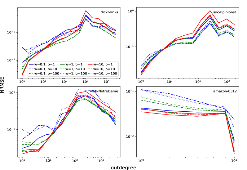
Figure 5: (visible in-edges, $c=1$) Effect of DUFS parameters on datasets with many connected components, when $B=0.1|V|$ and $c=1$. Legend shows the average budget per walker ($b$) and jump weight ($w$). Trade-off shows that configurations that result in many uniform node samples, such as $(w=10,b=1)$, yield accurate head estimates, whereas configurations such as $(w=1,b=10)$ yield accurate tail estimates.

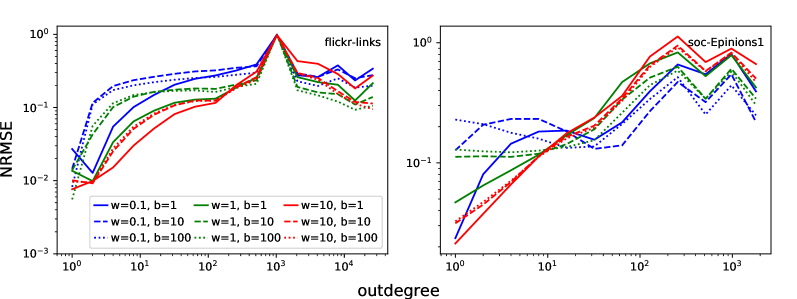
Figure 6: (invisible in-edges, $c=1$) Effect of DUFS parameters on datasets with many connected components, when $B=0.1|V|$ and $c=1$. Legend shows the average budget per walker ($b$) and jump weight ($w$). Configurations that result in many walkers which jump too often, such as $(w\geq 10,b=1)$ yield accurate head estimates, whereas configurations such as $(w=1,b=10^{3})$, yield accurate tail estimates.

Invisible in-edges, $c=1$

The results we obtained are similar to those obtained for the visible in-edge scenario, but NRMSEs tend to be larger. Figure 6 shows typical results for different DUFS parameters, represented by two datasets (also shown in the previous figure). Once again, the intuition for uniform edge sampling holds for the distribution head: decreasing $b$ and increasing $w$ yield more accurate estimates for the smallest out-degrees. While $b=1$ results in poor estimates for the largest out-degrees, our intuition regarding $w$ does not hold true for the tail. More precisely, in most cases $w=1$ outperforms $w=0.1$ (one exception being dataset soc-Epinions1). As opposed to the visible in-edge scenario, increasing $b$ tends to provide more accurate tail estimates for $w=1$. We investigate this effect in Section 5.3. We find that, for a fixed $w$, larger values of $b$ make the random walks jump more often, moving them from small volume components to large volume components, yielding better tail estimates.

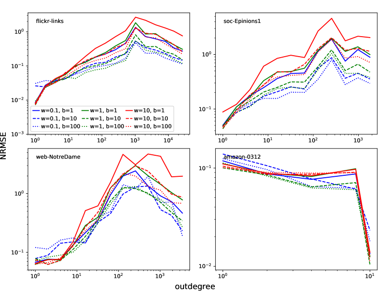
Figure 7: (visible in-edges, $c=10$) Effect of DUFS parameters on datasets with many connected components, when $B=0.1|V|$ and $c=1$. Legend shows the average budget per walker ($b$) and jump weight ($w$). Trade-off shows that configurations that result in many uniform node samples, such as $(w=10,b=1)$, yield accurate head estimates, whereas configurations such as $(w=1,b=10)$ yield accurate tail estimates.

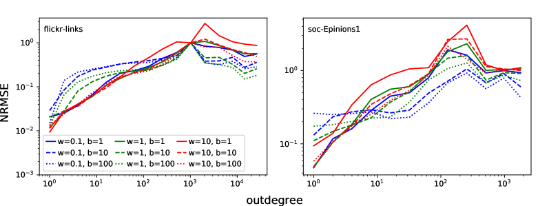
Figure 8: (invisible in-edges, $c=10$) Effect of DUFS parameters on datasets with many connected components, when $B=0.1|V|$ and $c=1$. Legend shows the average budget per walker ($b$) and jump weight ($w$). Configurations that result in many walkers which jump too often, such as $(w\geq 10,b=1)$ yield accurate head estimates, whereas configurations such as $(w=1,b=10^{3})$, yield accurate tail estimates.

Visible in-edges, $c=10$

Consider the case where the cost of obtaining uniform node samples is large, more precisely, 10 times larger than the cost of moving a walker. Figure 7 shows typical results for this setting. It is no longer clear that using many walkers and frequent random jumps achieves the most accurate head estimates, as this could rapidly deplete the budget. In fact, we observe that setting $w=10$ or $b=1$ yields poor estimates for both the smallest and largest out-degrees. While increasing the jump weight $w$ or decreasing $b$ sometimes improves estimates in the head, it rarely does so in the tail. The best results for the smallest out-degrees are often observed when setting $w=1$ and $b=10$ or $10^{2}$. On the other hand, setting $(w=0.1,b=10^{3})$ or $(w=1,b=10^{2})$ usually achieves relatively small NRMSEs for the largest out-degree estimates.

Invisible in-edges, $c=10$

Figure 8 shows typical results for this setting. Unlike the scenario with visible in-edges, setting $w=10$ and $b=1$ often produces the most accurate estimates for the smallest out-degrees. This is because many of the datasets have nodes with no out-edges; these nodes can only be reached through a neighbor or through random node sampling. Conversely, the general trends for tail estimates are similar to those observed for the visible in-edges case: large values of $w$ and small values of $b$ yield less accurate estimates for the largest out-degree values. For $w=1$, however, $b=10^{2}$ often outperforms $b=10^{3}$. On the other hand, for $w=0.1$ there is little difference in the estimates for different values of $b$.

5.2 Evaluation of DUFS in the visible in-edges scenario

In this section we compare two variants of Directed Unbiased Frontier Sampling: E-DUFS, which uses the edge-based estimator and DUFS, which uses the hybrid estimator, to each other and to a single random walk (SingleRW) and multiple independent random walks (MultiRW). We do not include Frontier Sampling in the comparison as it is a special case of DUFS where $w=0$ and we know from Section 5.1 that allowing random jumps effectively reduce estimation errors.

5.2.1 Out-degree and in-degree distribution estimates

Here we focus on estimating the marginal in- and out-degree distributions. Each simulation consists of 1000 runs from which we compute the empirical NRMSE. For MultiRW, E-DUFS and DUFS we set the average budget per walker to be $b=10$. For conciseness, we only show a few representative results.

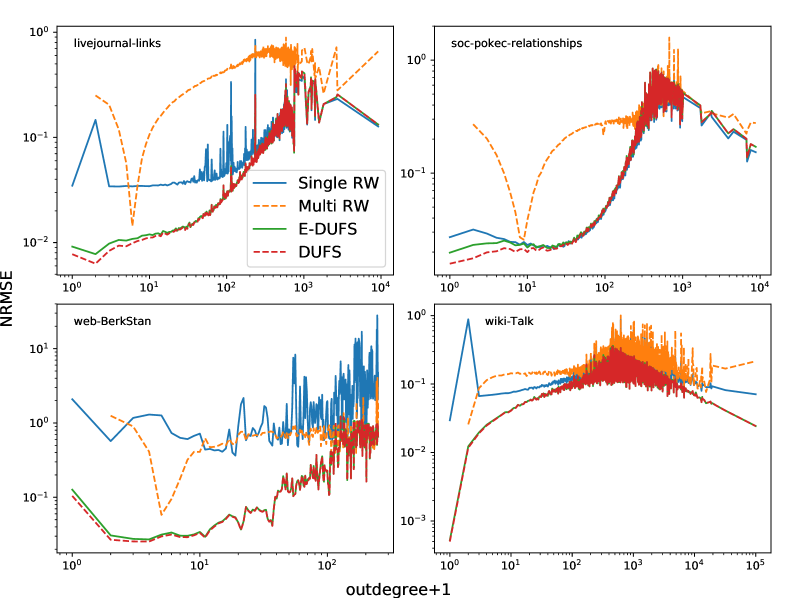
Figure 9: Comparison of single random walk (SingleRW), multiple independent random walks (MultiRW), DUFS with edge-based estimator (E-DUFS) and with hybrid estimator (DUFS). MultiRW yields the worst results, as the edge sampling probability is not the same across different connected components. Both DUFS variants outperform SingleRW, but DUFS is slightly more accurate in the head.

Figure 9 shows typical results obtained when using SingleRW, MultiRW, E-DUFS and DUFS to estimate out-degree distributions on the datasets. In 8 out of 15 datasets, MultiRW yields much larger NRMSEs than does the SingleRW. As pointed out in [Ribeiro and Towsley (2010), Section 4.5], this is due to the fact that the estimator in (1) assumes that all edges are sampled with the same probability. This assumption is violated by MultiRW because the stationary sampling probability depends on the size of the connected component within which each walker is located. E-DUFS estimates are consistently more accurate than those of MultiRW and SingleRW, except on datasets where the original graph and its LCC have similar out-degree distributions. In some of these cases SingleRW slightly outperforms E-DUFS in the tail (see top-right fig.). DUFS, in turn, outperforms E-DUFS in the head of the out-degree distribution and has similar performance when estimating other out-degree values. For this reason, defining the estimation task in terms of the CCDF would give DUFS an unfair advantage.

When restricted to the largest connected component, the performance differences between SingleRW and E-DUFS and those between SingleRW and DUFS become smaller, for $B=0.1|V|$. Results for in-degree distribution estimation are qualitatively similar and are omitted.

5.2.2 Joint in- and out-degree distributions

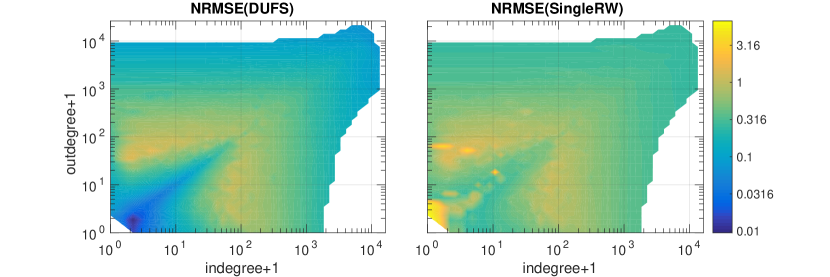
(a) flickr-links

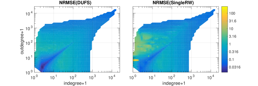
(b) youtube-links

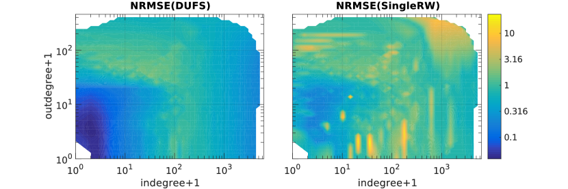
(c) web-Google

Figure 10: Comparison between DUFS and SingleRW w.r.t. NRMSE when estimating the joint in- and out-degree distribution. In most cases SingleRW will exhibit “hot spots” (regions with large NRMSE), which are mitigated by DUFS.

We compare the NRMSEs associated with DUFS and SingleRW for the estimates of the joint in- and out-degree distribution. We observe that DUFS consistently outperforms SingleRW on all datasets. On 10 out of 15 datasets, the estimates corresponding to low in-degree and low out-degree exhibit much smaller errors when using DUFS than when using SingleRW. Furthermore, DUFS also achieves smaller estimation errors for most of the remaining points of the joint distribution in 11 out of 15 datasets. Figures 10(a-b) show heatmaps corresponding to typical NRMSE results for DUFS and SingleRW. Interestingly, we note that on the web graph datasets and on the email-EuAll dataset, DUFS outperforms SingleRW by one or two orders of magnitude, as illustrated by Figure 10(c), which shows the heatmap comparison for dataset web-Google. Although the NRMSE exhibited by SingleRW applied to the LCC datasets is much smaller, the comparison between DUFS and SingleRW is qualitatively similar and is, therefore, omitted.

We then investigated the performance gains obtained by using the hybrid estimator instead of the original estimator. Figures 11(a-b) show the ratios between the NRMSEs obtained with DUFS (hybrid) to those obtained with the E-DUFS (original) for two networks. We chose to use the NRMSE ratio (or equivalently, the root MSE ratio) to make it easier to visualize the differences. We observe that DUFS consistently outperforms E-DUFS on all datasets. More precisely, the error ratio is rarely above one and, for points corresponding to small in- and out-degrees, it often lies below 0.9. Results on most datasets are similar to that depicted in Figure 11(a), but results on social networks datasets are closer to that shown in Figure 11(b), where large in- and out-degrees also seem to benefit from the information contained in the walkers’ initial locations. Results for the LCC datasets are qualitatively similar, with accuracy gains from the hybrid estimator slightly larger on these datasets than on the original datasets.

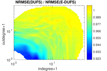
(a) p2p-Gnutella31

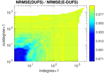
(b) soc-Slashdot0902

Figure 11: NRMSE ratios between DUFS and E-DUFS of the estimated joint in- and out-degree distribution for two datasets. DUFS is typically better than E-DUFS at low in and out-degree regions (left), but in social network graphs presented improvements over most of the joint distribution (right).

5.3 Evaluation of DUFS in the invisible in-edges scenario

In this section, we compare the NRMSEs associated with DUFS and Directed Unbiased Random Walk (DURW) method when estimating out-degree distributions in the case where in-edges are not directly observable. We note that DURW is known to outperform a reference method for this scenario proposed in [Bar-Yossef and Gurevich (2008)]. For a comparison between DURW and this reference method, please refer to [Ribeiro et al. (2012)].

As we mentioned in Section 5.1, DURW results are similar to those obtained with DUFS when the budget per walker $b$ is large, since DURW is a special case of DUFS where $b=B-c$. Therefore, we focus on comparing DUFS for small values of $b$ and DURW, when the total number of uniform node samples collected by each method is roughly the same. More precisely, we simulate DUFS for $b=10$ and $w=1$ and set the DURW parameter $w$ so that the number of node samples differs by at most 1% (averaged over 1000 runs). This aims to provide a fair comparison between these methods.

We find that neither of the two methods consistently outperforms the other over all datasets. The extra random jumps performed by DURW will prevent the walker from spending much of the budget in small volume components. As a result, DURW tends to exhibit larger errors in the head but smaller errors in the tail of the out-degree distribution than DUFS. Figure 12 show typical results for $w=1$ and $b=10$. DUFS exhibited lower estimation errors in the head of the distribution on 11 datasets, being outperformed by DURW on one dataset and displaying comparable performance on the others. In 6 out of 15 datasets, DURW had better performance in the tail, while DUFS yielded better results on other five datasets. Results for $w=1$ and $b\in\{10^{2},10^{3}\}$ are similar and are, therefore, omitted. As $b$ increases, differences between DUFS and DURW start to vanish.

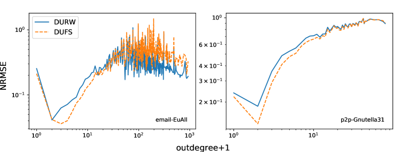
Figure 12: NRMSEs associated with DUFS ($w=1$, $b=10$) and DURW ($w^{\prime}$ chosen to match average number of node samples) when estimating out-degree distribution. DURW performs more random jumps, thus better avoiding small volume components. This improves DURW results in the tail, but often results in lower accuracy in the head (left). In one third of the datasets, DUFS yielded similar or better results than DURW over most out-degree points (right).

Figure 13: NRMSEs associated with DUFS ($w=1$, $b=10$) and DURW ($w^{\prime}$ chosen to match average number of node samples) when estimating out-degree distribution.

To better understand the impact of multiple connected components in DUFS and DURW performances, we simulate each method on the largest strongly connected component of each dataset (i.e., on the LCC datasets). Figure 13 shows typical results among the LCC datasets. In most networks, DUFS yields smaller NRMSE than DURW in the head and yield similar results in the tail. Once again, for larger $b$ the performances of DUFS and DURW become equivalent.

5.4 Relationship between NRMSE and out-degree distribution

Throughout Section 5 we observed that the NRMSE associated with RW-based methods tends to increase with out-degree up to a certain out-degree and to decrease after that. Moreover, for some out-degree ranges the $\log$ NRMSE seems to vary linearly with the $\log$ out-degree. Figure 5). For simplicity, we discuss the undirected graph case, but the extension to directed graphs is straightforward. The RW methods discussed here combine uniform node sampling with RW sampling approximated as uniform edge sampling. For simplicity, we analyze below the accuracy of uniform node and uniform edge sampling. We assume that each sampled edge produces one observation, obtained by retrieving the set of labels associated with one of the adjacent vertices chosen equiprobably. Therefore both node sampling and edge sampling collect node labels.

Let $\mathbb{S}=\{s_{1},\ldots,s_{B}\}$ be the sequence of sampled vertices. For uniform node sampling, the probability of observing a given label $\ell$ in $\mathcal{L}(s_{i})$ is $\theta_{\ell}$, for any $i=1,\ldots,B$. The minimum variance unbiased estimator of $\theta_{\ell}$ is

$$T_{\textrm{vs}}^{\ell}(\mathbb{S})=\frac{1}{B}\sum_{i=1}^{B}{\mathds{1}}\{\ell\in\mathcal{L}(s_{i})\}.$$ (9)

Note that the summation in (9) is binomially distributed with parameters $B$ and $\theta_{\ell}$. It follows that the mean squared error (MSE) of $T^{\ell}_{\textrm{vs}}(\mathbb{S})$ is

$$\mbox{MSE}(T^{\ell}_{\textrm{vs}}(\mathbb{S})) =E[(T^{\ell}_{\textrm{vs}}(\mathbb{S})-\theta_{\ell})^{2}],$$

$$=\frac{1}{B}\theta_{\ell}(1-\theta_{\ell}).$$ (10)

For uniform edge sampling, the probability of observing a given label $\ell\in\mathcal{L}$ in the sample $\mathcal{L}(s_{i})$ for $i=1,\ldots,B$, equals

$$\pi_{\ell}=\frac{\sum_{v\in V}{\mathds{1}}\{\ell\in\mathcal{L}(v)\}\deg(v)}{\sum_{u\in V}\deg(u)}.$$

In that case, the following estimator can be shown to be asymptotically unbiased

$$T^{\ell}_{\textrm{es}}(\mathbb{S})=\frac{1}{B}\frac{\sum_{k=1}^{B}{\mathds{1}}\{\ell\in\mathcal{L}(s_{k})\}\deg^{-1}(s_{k})}{\sum_{j=1}^{B}\deg^{-1}(s_{j})}.$$ (11)

In particular, when node labels are the undirected degrees of each node, the probability of observing a given degree $d$ becomes $\pi_{d}=d\theta_{d}/\bar{d}$, where $\bar{d}$ is the average undirected degree. The estimator for $B=1$ reduces to $T^{d}_{\textrm{es}}(\mathcal{S}_{1})={\mathds{1}}\{s_{1}=d\}$, which is a random variable distributed according to a Bernoulli with parameter $\pi_{d}$. As a result, the MSE for $B>1$ independent samples is

$$\mbox{MSE}(T^{d}_{\textrm{es}}(\mathbb{S})) = \frac{1}{B}\pi_{d}(1-\pi_{d})=\frac{1}{B}\frac{d\theta_{d}}{\bar{d}}\left(1-\frac{d\theta_{d}}{\bar{d}}\right)$$ (12)

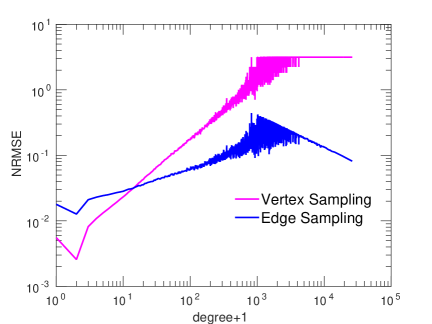
Figure 14: NRMSE associated with uniform node sampling and uniform edge sampling when estimating degree distribution of the Flickr dataset (for $B=0.1|V|$).

Equations (10) and (12) characterize the conditions under which each sampling model is more accurate. More precisely, for all $i$ such that $\theta_{d}>\pi_{d}$ (or equivalently, $d<\bar{d}$), uniform node sampling yields better estimates than uniform edge sampling. This dichotomy is illustrated in Figure 14, which shows the NRMSE associated with degree distribution estimates resulting from each sampling model on the flickr-links dataset, for $B=0.1|V|$.

Note that in log-log scale, both curves resemble a straight line for $d=2,\ldots,10^{3}$, which indicates a power law. For degrees larger than $5\times 10^{3}$, the NRMSE associated with node sampling is constant, while the NRMSE associated with edge sampling decreases linearly with the degree. We show that these observations are direct consequences of the fact that the degree distribution in this network (as well as many other real networks) approximately follows a power law distribution. However, the degree distribution of a finite network cannot be an exact power law distribution because the tail is truncated. As a result, most of the largest degree values are observed exactly once. This can be seen in Figure 4 by noticing that on the flickr-links (and many other datasets) the p.m.f. is constant for the largest out-degrees. Assume, for instance, that the degree distribution can be modeled as

$$\theta_{d}=\begin{cases}d^{-\beta}/Z\,,&1\leq d\leq\tau\\ 1/|V|\,,&d>\tau,\end{cases}$$

for some $\beta\geq 1$ and some normalizing constant $Z$.

From (10), we have for uniform node sampling,

$$\mbox{NRMSE}(T^{d}_{\textrm{vs}}(\mathbb{S}))=\sqrt{(1/\theta_{d}-1)/B}.$$ (13)

For $\theta_{d}\ll 1$, this implies

$$\mbox{NRMSE}(T^{d}_{\textrm{vs}}(\mathbb{S}))\approx\begin{cases}\sqrt{Zd^{\beta}/B}\,,&1\leq d\leq\tau\\ \sqrt{|V|/B}\,,&d>\tau.\end{cases}$$

For $d>\tau$, the NRMSE is constant. Otherwise, taking the log on both sides yields

$$\log(\mbox{NRMSE}(T^{d}_{\textrm{vs}}(\mathbb{S})))\approx\frac{\beta}{2}\log d+\frac{1}{2}(\log Z-\log B),\;1\leq d\leq\tau,$$ (14)

which explains the relationship observed for uniform node sampling in Fig. 14.

From (12), we have for uniform edge sampling,

$$\mbox{NRMSE}(T^{d}_{\textrm{es}}(\mathbb{S}))=\sqrt{(1/\pi_{d}-1)/B}.$$ (15)

For $\theta_{d}\ll 1$, this implies

$$\mbox{NRMSE}(T^{d}_{\textrm{es}}(\mathbb{S}))\approx\begin{cases}\sqrt{Z\bar{d}d^{\beta-1}/B}\,,&1\leq d\leq\tau\\ \sqrt{\frac{|E|}{d}/B}\,,&d>\tau.\end{cases}$$

Taking the log on both sides, it follows that

$$\log(\mbox{NRMSE}(T^{d}_{\textrm{es}}(\mathbb{S})))\approx\begin{cases}\frac{\beta-1}{2}\log d+\frac{1}{2}(\log Z+\log\bar{d}-\log B)\,,&1\leq d\leq\tau\\ -\frac{1}{2}\left(\log d-\log|E|-\log B\right)\,,&d>\tau,\end{cases}$$ (16)

which explains the linear increase followed by the linear decrease observed in Fig. 14. Although some RW-based methods can collect uniform node samples (e.g., via random jumps), NRMSE trends for large degrees are better described by (16) than by (14), since most of the information about these degrees comes from RW samples.

6 Results on node label distributions estimation

This section focuses on network datasets which possess (non-topological) node labels. Using these datasets, all of which represent undirected networks, we investigate which combinations of DUFS parameters outperform uniform node sampling when estimating node label distributions of the top 10% largest degree nodes. These nodes often represent the most important objects in a network.

Two of the four undirected attribute-rich datasets we use are social networks (DBLP and LiveJournal) obtained from Stanford SNAP, while two are information networks (DBpedia and Wikipedia) obtained from CMU’s Auton Lab GitHub repository active-search-gp-sopt  [Ma et al. (2015)]. In these datasets, node labels correspond to some type of group membership and a node is allowed to be part of multiple groups simultaneously. Figure 15 shows, on the left, the degree distribution for each network. On the right, it displays the relative frequency of each attribute in decreasing order (blue bars/dots) along with attribute frequency among the top 10% largest degree nodes (red bars/dots).

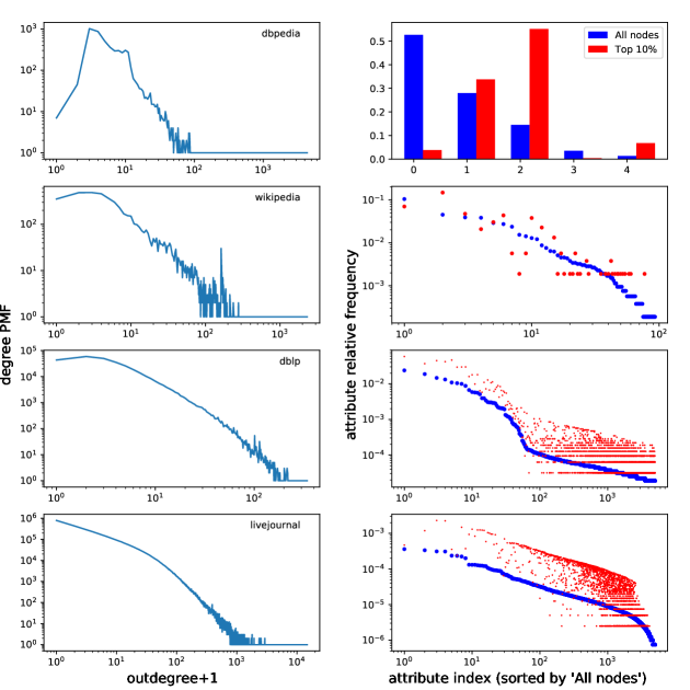
Figure 15: Degree and node attribute distribution for undirected attribute-rich networks.

We simulate 1000 DUFS runs on each undirected network for all combinations of random jump weight $w\in\{0.1,1,10\}$ and budget per walker $b\in\{1,10,10^{2}\}$. Figure 16 compares the NRMSE associated with DUFS for different parameter combinations against uniform node sampling. Uniform node sampling results are obtained analytically using eq. (13). On DBpedia, Wikipedia and DBLP, almost all DUFS configurations outperform uniform node sampling. On LiveJournal, node sampling outperforms DUFS for attributes associated with large probability masses, but underperforms DUFS for attributes with smaller masses. In summary, we observe that DUFS with $w\in\{0.1,1.0\}$ and $b\in\{10,10^{2}\}$ yields superior accuracy than uniform node sampling when estimating node label distributions among the top 10% largest degree nodes.

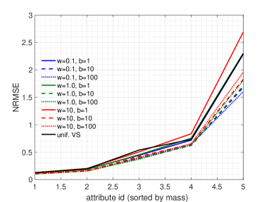
(a) DBpedia

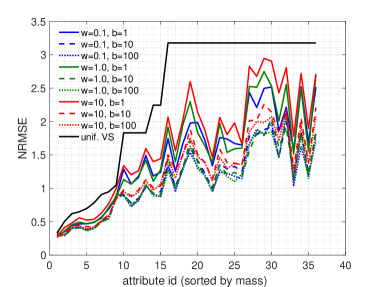
(b) Wikipedia

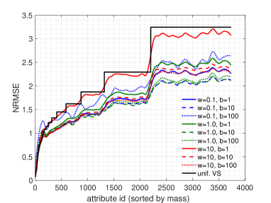
(c) DBLP

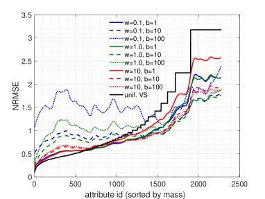
(d) LiveJournal

Figure 16: Comparison of hybrid estimator (DUFS) with uniform node sampling. DUFS curves on DBLP plot are smoothed by a local regression using weighted linear least squares and a second degree polynomial model to avoid clutter. DUFS with $w\in\{0.1,1.0\}$ and $b\in\{10,10^{2}\}$ yields comparable or superior accuracy than uniform node sampling.

7 Discussion: DUFS performance in the absence of uniform node sampling

In this section, we investigate the estimation accuracy of {E,H}-DUFS when random walkers are not initialized uniformly over $V$. We consider two simple non-uniform distributions over $V$ to determine the initial walker locations walker positions:

• Distribution Prop: proportional to the undirected degree, that is,

  $$P(\textrm{initial walker location is }v)=\frac{\deg(v)}{\sum_{u\in V}\deg(u)};$$ (17)

• Distribution Inv: proportional to the reciprocal of the undirected degree, that is,

  $$P(\textrm{initial walker location is }v)=\frac{\deg^{-1}(v)}{\sum_{u\in V}\deg^{1}(u)}.$$ (18)

We simulate E-DUFS and DUFS on each network dataset setting the budget per walker to $b\in\{1,10,10^{2},B-1\}$ in a scenario where in-edges are visible, performing 100 runs. Note that $b=B-1$ corresponds to the case of a single random walker. Since we assume uniform node sampling (VS) is not available, we must set the random jump weight to $w=0$. We include, however, results obtained when the initial walker locations are determined via VS for comparison. Figure 17 shows typical values of NRMSE associated with E-DUFS out-degree distribution estimates. We observe that NRMSE decreases with the budget per walker until $b=10^{2}$, both for Prop and Inv. Simulations for the case of a single walker ($b=B-1$) yielded poor results and are omitted.

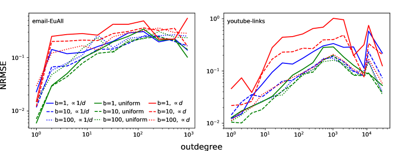
Figure 17: Effect of initializing walkers non-uniformly over $V$ on E-DUFS accuracy. NRMSE decreases with budget per walker until $b=10^{2}$.

Intuitively, using the hybrid estimator when the initial walker locations come from some non-uniform distribution can incur unknown – and potentially large – biases. We conducted a set of simulations with DUFS, which corroborated this intuition. These results are omitted for conciseness.

In summary, our results indicate that when the initial walker locations are determined according to some unknown distribution, a practitioner should use E-DUFS with moderately large $b$ (e.g., $10^{2}$).

8 Related Work

Crawling methods for exploring undirected graphs: A number of papers investigate crawling methods (e.g., breadth-first search, random walks, etc.) for generating subgraphs with similar topological properties as the underlying network [Leskovec and Faloutsos (2006), Hubler et al. (2008)]. On the other hand, [Maiya and Berger-Wolf (2011)] empirically investigates the performance of such methods w.r.t. specific measures of representativeness that can be useful in the context of specific applications (e.g., finding high-degree nodes for outbreak detection). However, these works focus on techniques that yield biased samples of the network and do not possess any accuracy guarantees. [Achlioptas et al. (2009), Kurant et al. (2011b)] demonstrate that Breadth-First-Search (BFS) introduces a large bias towards high degree nodes, and that is difficult to remove these biases in general, although they can be reduced if the network in question is almost random [Kurant et al. (2011b)]. Random walk (RW) is biased to sample high degree nodes, however its bias is known and can be easily corrected [Ribeiro and Towsley (2010)]. Random walks in the form of Respondent Driven Sampling (RDS) [Heckathorn (2002), Salganik and Heckathorn (2004)] have been used to estimate population densities using snowball samples of sociological studies. The Metropolis-Hasting RW (MHRW) [Stutzbach et al. (2009)] modifies the RW procedure to adjust for degree bias, in order to obtain uniform node samples. [Ribeiro and Towsley (2012), Chiericetti et al. (2016)] analytically prove that MHRW degree distribution estimates perform poorly in comparison to RWs. Empirically, the accuracy of RW and MHRW has been compared in [Rasti et al. (2009), Gjoka et al. (2010)] and, as predicted by the theoretical results, RW is consistently more accurate than MHRW.

Reducing the mixing time of a regular RW is one way of improving the performance of RW based crawling methods. [Avrachenkov et al. (2010)] proves that random jumps increase the spectral gap of the random walk, which in turn, leads to faster convergence to the steady state distribution. [Kurant et al. (2011a)] assigns weights to nodes that are computed using their neighborhood information, and develop a weighted RW-based method to perform stratified sampling on social networks. They conduct experiments on Facebook and show that their stratified sampling technique achieves higher estimation accuracy than other methods. However, the neighborhood information in their method is limited to helping find random walk weights and is not used in the estimation of graph statistics of interest. To solve this problem, [Dasgupta et al. (2012)] randomly samples nodes (either uniformly or with a known bias) and then uses neighborhood information to improve its unbiased estimator. [Zhou et al. (2016)] modifies the regular random walk by “rewiring” the network of interest on-the-fly in order to reduce the mixing time of the walk.

Crawling methods for exploring directed graphs: Estimating observable characteristics by sampling a directed graph (in this case, the Web graph) has been the subject of [Bar-Yossef and Gurevich (2008)] and [Henzinger et al. (2000)], which transform the directed graph of web-links into an undirected graph by adding reverse links, and then use a MHRW to sample webpages uniformly. The DURW method proposed in [Ribeiro et al. (2012)] adapts the “backward edge traversal” of [Bar-Yossef and Gurevich (2008)] to work with a pure random walk and random jumps. Both of these Metropolis-Hastings RWs ([Bar-Yossef and Gurevich (2008)] and [Henzinger et al. (2000)]) are designed to sample directed graphs and do not allow random jumps. However, the ability to perform random jumps (even if jumps are rare) makes DURW and DUFS more efficient and accurate than the MetropolisHastings RW algorithm. Random walks with PageRank-style jumps are used in [Leskovec and Faloutsos (2006)] to sample large graphs. In [Leskovec and Faloutsos (2006)], however, no technique is proposed to remove the large biases induced by the random walk and the random jumps, which makes this method unfit for estimation purposes. More recently, another method based on PageRank was proposed in [Salehi and Rabiee (2013)], but it assumes that obtaining uniform node samples is not feasible. In the presence of multiple strongly connected components, this method offers no accuracy guarantees.

In the last decade, there has been a growing interest in graph sketching for processing massive networks. A sketch is a compact representation of data. Unlike a sample, a sketch is computed over the entire graph, that is observed as a data stream. For a survey on graph sketching techniques, please refer to [McGregor (2014)].

9 Conclusion

In this paper, we proposed the Directed Unbiased Frontier Sampling (DUFS) method for characterizing networks. DUFS generalizes the Frontier Sampling (FS) and the Directed Unbiased Random Walk (DURW) methods. DUFS extends FS to make it applicable to directed networks when incoming edges are not directly observable by building on ideas from DURW. DUFS adapts DURW to use multiple coordinated walkers. Like DURW, DUFS can also be applied to undirected networks without any modification.

We also proposed a novel estimator for node label distribution that can account for FS and DUFS walkers initial locations – or more generally, uniform node samples – and a heuristic that can reduce the variance incurred by node samples that happen to sample nodes whose labels have extremely low probability masses. When the proposed estimator is used in combination with the heuristic, we showed that estimation errors can be significantly reduced in the distribution head when compared with the estimator proposed in [Ribeiro and Towsley (2010)], regardless of whether we are estimating out-degree, in-degree or joint in- and out-degree distributions.

We conducted an empirical study on the impact of DUFS parameters (namely, budget per walker and random jump weight) on the estimation of out-degree and in-degree distributions using a large variety of datasets. We considered four scenarios, corresponding to whether incoming edges are directly observable or not and whether uniform node sampling has a similar or larger cost than moving random walkers on the graph. This study allowed us to provide practical guidelines on setting DUFS parameters to obtain accurate head estimates or accurate tail estimates. When the goal is a balance between the two objectives, intermediate configurations can be chosen.

Last, we compared DUFS with random walk-based methods designed for undirected and directed networks. In our simulations for the scenario where in-edges are visible, DUFS yielded much lower estimation errors than a single random walk or multiple independent random walks. We also observed that DUFS consistently outperforms FS due to the random jumps and use of the improved estimator. In the scenario where in-edges are unobservable, DUFS outperformed DURW when estimating the probability mass associated with the smallest out-degree values (for equivalent parameter settings). In addition, more often than not, DUFS slightly outperformed DURW when estimating the mass associated to the largest out-degrees. In the presence of multiple strongly connected components, DURW tends to move from small to largest components more often than DUFS, sometimes exhibiting lower estimation errors in the distribution tail. However, when restricting the estimation to the largest component, DUFS outperforms DURW in virtually all datasets used in our simulations.

Appendices

Appendix A Hybrid estimator and its statistical properties

Let us recall variables and constants used in the definition of the hybrid estimator:

$n_{i}$	number of node samples with label $i$
$\theta_{i,j}$	fraction of nodes in $G^{(t)}$ with label $i$ and undirected degree $j$
$m_{i,j}$	number of edge samples with label $i$ and bias $j$
$m_{i}=\sum_{j}m_{i,j}$	total number of edge samples with label $i$
$N=\sum_{i}n_{i}$	total number of node samples
$M=\sum_{i}m_{i}$	total number of edge samples
$B=N+M$	total budget

In this appendix, we derive the recursive variant of the hybrid estimator. From that we derive its non-recursive variant. Next, we show that the non-recursive variant is asymptotically unbiased. In the case of undirected networks where the average degree is given, we show that the resulting hybrid estimator of the undirected degree mass is the minimum variance unbiased estimator (MVUE).

We approximate random walk samples in DUFS by uniform edge samples from $G_{u}$. Experience from previous papers shows us that this approximation works very well in practice. This yields the following likelihood function

$$L({\boldsymbol{\theta}}|\mathbf{n},\mathbf{m})=\frac{\prod_{i}\theta_{i}^{n_{i}}\prod_{k}(k\theta_{i,k})^{m_{i,k}}}{\left(\sum_{s,t}t\theta_{s,t}\right)^{M}}.$$ (19)

The key idea in our derivation is that we can bypass the numerical estimation of the $\theta_{i,j}$’s by noticing that $\theta_{i,j}\propto\theta_{i}$, $\theta_{i,j}\propto m_{i,j}$ and $\theta_{i,j}\propto 1/j$. Hence, the maximum likelihood estimator of $\theta_{i,j}$ for $j=1,\ldots,Z$ is the Horvitz-Thompson estimator

$$\hat{\theta}_{i,j}=\frac{\theta_{i}m_{i,j}}{j\mu_{i}},$$ (20)

where $\mu_{i}=\sum_{k}m_{i,k}/k$.

Substituting (20) in (19) yields

$$L({\boldsymbol{\theta}}|\mathbf{n},\mathbf{m})=\frac{\prod_{i}\theta_{i}^{n_{i}}\prod_{k}(\theta_{i}m_{i,k}/\mu_{i})^{m_{i,k}}}{\left(\sum_{s}\theta_{s}\sum_{z}m_{s,z}/\mu_{s}\right)^{M}}.$$ (21)

The log-likelihood approximation is then given by

$$\mathcal{L}({\boldsymbol{\theta}}|\mathbf{n},\mathbf{m})=-M\log\left(\sum_{s}\theta_{s}\sum_{z}\frac{m_{s,z}}{\mu_{s}}\right)+\sum_{i}n_{i}\log\theta_{i}+\sum_{k}m_{i,k}(\log\theta_{i}+\log m_{i,k}-\log\mu_{i}).$$ (22)

We rewrite $\theta_{i}$ as $e^{\beta_{i}}/\sum_{j}e^{\beta_{j}}$ to account for the distribution constraints $\sum_{i}\theta_{i}=1$ and $\theta_{i}\in[0,1]$. Hence, we have

$$\mathcal{L}({\boldsymbol{\beta}}|\mathbf{n},\mathbf{m})=-M\log\left(\sum_{s}\frac{e^{\beta_{s}}m_{s}}{\mu_{s}}\right)+\sum_{i}(n_{i}+m_{i})\beta_{i}-N\log\left(\sum_{j}e^{\beta_{j}}\right)+C,$$ (23)

where $m_{i}=\sum_{k}m_{i,k}$ and $C$ is a constant that does not depend on $\beta$.

The partial derivative w.r.t. $\beta_{i}$ is given by

$$\frac{\partial\mathcal{L}({\boldsymbol{\beta}}|\mathbf{n},\mathbf{m})}{\partial\beta_{i}}=-\frac{Me^{\beta_{i}}m_{i}/\mu_{i}}{\sum_{s}e^{\beta_{s}}m_{s}/\mu_{s}}+n_{i}+m_{i}-\frac{Ne^{\beta_{i}}}{\sum_{j}e^{\beta_{j}}}.$$ (24)

Setting $\partial\mathcal{L}({\boldsymbol{\beta}}|\mathbf{n},\mathbf{m})/\partial\beta_{i}=0$ and substituting back $\theta_{i}$ yields

$$\theta_{i}^{\star} = \frac{n_{i}+m_{i}}{N+M\frac{m_{i}/\mu_{i}}{\sum_{s}\theta_{s}^{\star}m_{s}/\mu_{s}}}.$$ (25)

Theorem 1.

Let $N=cB$ and $M=(1-c)B$, for some $0<c<1$. The estimator

$$\hat{\theta}_{i}=\frac{n_{i}+m_{i}}{N+M\frac{m_{i}}{\mu_{i}\hat{d}}},$$ (26)

where $\mu_{i}=\sum_{k}m_{i,k}/k$ and $\hat{d}=M/\sum_{i}\mu_{i}$, is an asymptotically unbiased estimator of $\theta_{i}$.

Proof A.1.

In the limit as $B\rightarrow\infty$, we have

$$E[n_{i}]=N\theta_{i},\qquad E[m_{i,k}]=M\frac{k\theta_{i,k}}{\sum_{s,l}l\theta_{sl}},\qquad E[m_{i}]=M\frac{\sum_{k}k\theta_{i,k}}{\sum_{s,l}l\theta_{s,l}},$$

and thus,

$$E[\mu_{i}]=M\frac{\sum_{k}k\theta_{i,k}/k}{\sum_{s,l}l\theta_{sl}}=M\frac{\theta_{i}}{\sum_{s,l}l\theta_{sl}}\quad\textrm{and}\quad E\left[\frac{m_{i}}{\mu_{i}}\right]=\frac{\sum_{k}k\theta_{i,k}}{\theta_{i}}.$$

It follows that

$$\lim_{B\rightarrow\infty}E[\hat{d}] = \frac{M}{M\frac{\sum_{i}\theta_{i}}{\sum_{s,l}l\theta_{sl}}}=\sum_{s,l}l\theta_{sl}.$$

Substituting the above in eq. (26), we have

$$\lim_{B\rightarrow\infty}E[\theta_{i}^{\star}]=\frac{N\theta_{i}+M\frac{\sum_{k}k\theta_{i,k}}{\sum_{s,l}l\theta_{s,l}}}{N+M\frac{\sum_{k}k\theta_{i,k}/\theta_{i}}{\sum_{s,l}l\theta_{s,l}}}=\theta_{i}.$$

This concludes the proof.

In Section 4.2.2 we mentioned a special case of the previous estimator, where the node label is the undirected degree itself. We prove that this estimator, denoted by $\hat{\theta}_{i}$ is the minimum variance unbiased estimator (MVUE) of $\theta_{i}$.

Theorem 2.

The estimator

$$\bar{\theta}_{i}=\frac{n_{i}+m_{i}}{N+Mi/\bar{\mu}},$$

where $\bar{\mu}=\sum_{j}j\theta_{j}$, is an unbiased estimator of $\theta_{i}$.

Proof A.2.

We know that $n_{i}\sim\mathrm{Binomial}(N,\theta_{i})$ and $m_{i}\sim\mathrm{Binomial}(M,i\theta_{i}/\bar{\mu})$. Hence,

$$E[\hat{\theta}_{i}] = \sum_{n_{i},m_{i}}\frac{n_{i}+m_{i}}{N+Mi/\bar{\mu}}\overbrace{\binom{N}{n_{i}}\theta_{i}^{n_{i}}(1-\theta_{i})^{N-n_{i}}}^{A(n_{i})}\overbrace{\binom{M}{m_{i}}\left(\frac{i\theta_{i}}{\bar{\mu}}\right)^{m_{i}}\left(1-\frac{i\theta_{i}}{\bar{\mu}}\right)^{M-m_{i}}}^{B(m_{i})}$$

$$= \frac{1}{N+Mi/\bar{\mu}}\left(\sum_{n_{i}}n_{i}A(n_{i})\sum_{m_{i}}B(m_{i})+\sum_{m_{i}}m_{i}B(m_{i})\sum_{n_{i}}A(n_{i})\right)$$

$$= \frac{1}{N+Mi/\bar{\mu}}\left(\sum_{n_{i}}n_{i}A(n_{i})+\sum_{m_{i}}m_{i}B(m_{i})\right)$$

$$= \frac{1}{N+Mi/\bar{\mu}}\left(N\theta_{i}+Mi\theta_{i}/\bar{\mu}\right)$$

$$= \theta_{i}.$$

Having proved that $\hat{\theta}_{i}$ is unbiased, we are now ready to show that it is also the minimum variance unbiased estimator (MVUE). In order to do so, we prove Lemmas A.3 and A.6 that show respectively that $n_{i}+m_{i}$ is a sufficient and complete statistic of $\theta_{i}$.

Lemma A.3.

The statistic $n_{i}+m_{i}$ is a sufficient statistic with respect to the likelihood of $\theta_{i}$.

Proof A.4.

The log-likelihood equation for estimator (7) is given by

$$L({\boldsymbol{\theta}}|\mathbf{n},\mathbf{m}) = \frac{\prod_{i}\theta_{i}^{n_{i}}\prod_{j}(j\theta_{j})^{m_{j}}}{\hat{\mu}^{M}}$$ (27)

$$= \frac{\prod_{j}j^{m_{j}}}{\hat{\mu}^{M}}\prod_{i}\theta_{i}^{n_{i}+m_{i}}.$$

We can see from eq. (27) that the likelihood function $L({\boldsymbol{\theta}}|\mathbf{n},\mathbf{m})$ can be factored into a product such that one factor, $\prod_{j}j^{m_{j}}/\hat{\mu}^{M}$, does not depend on $\theta_{i}$ and the other factor, which does depend on $\theta_{i}$, depends on $\mathbf{n}$ and $\mathbf{m}$ only through $n_{i}+m_{i}$. From the Fisher-Neyman factorization Theorem [Lehmann et al. (1991)], we conclude that $n_{i}+m_{i}$ is a sufficient statistic for the distribution of the sample.

We now prove that $n_{i}+m_{i}$ is also a complete statistic for the distribution of the sample.

Definition A.5.

Let $X$ be a random variable whose probability distribution belongs to a parametric family of probability distributions $P_{\theta}$ parametrized by $\theta$. The statistic $s$ is said to be complete for the distribution of $X$ if for every measurable function $g$ (which must be independent of $\theta$) the following implication holds:

$$E(g(s(X)))=0\ \textrm{for all }\mbox{$\theta$}\Rightarrow P_{\theta}(g(s(X))=0)=1\ \textrm{for all }\theta.$$

Lemma A.6.

The statistic $n_{i}+m_{i}$ is a complete statistic w.r.t. the likelihood of $\theta_{i}$.

Proof A.7.

$$E[g(n_{i}+m_{i})] = 0$$

$$\sum_{n_{i},m_{i}}g(n_{i}+m_{i})P_{\theta}(n_{i},m_{i}) = 0$$

$$\sum_{n_{i},m_{i}}g(n_{i}+m_{i})A(n_{i})B(m_{i}) = 0$$ (28)

The LHS of (28) is a polynomial of degree $M+N$ on $\theta_{i}$. Hence, it can be written as

$$C_{0}+C_{1}\theta_{i}+C_{2}\theta_{i}^{2}+\ldots+C_{N+M}\theta_{i}^{N+M}=0.$$ (29)

We prove that $P_{\theta}(g(s(X))=0)=1\ \textrm{for all }\theta$ by contradiction. Suppose that there is a $\theta$ such that $P_{\theta}(g(s(X))\neq 0)>0$. In order to have $E(g(s(X)))=0$, there must be terms for which $g(.)$ is strictly positive and terms for which $g(.)$ is strictly negative. Let $g(h_{1})$ be the smallest $h_{1}$ such that $g(h_{1})>0$. Let $g(h_{2})$ be the smallest $h_{2}$ such that $g(h_{2})<0$. Let $h=\min(h_{1},h_{2})$.

Expanding $A(n_{i})B(m_{i})$ in eq. (28) we note that the degree of the resulting polynomial is at least $n_{i}+m_{i}$ on $\theta_{i}$. Therefore, the coefficient $C_{h}$ in eq. (29) associated with $\theta_{i}^{h}$ cannot have terms of $g(.)$ larger than $h$. Then $C_{h}$ can only be zero if $h_{1}=h_{2}$ which is a contradiction.

Theorem 3.

The unbiased estimator $\bar{\theta}_{i}$ is the minimum variance unbiased estimator (MVUE) of $\theta_{i}$.

Proof A.8.

According to the Lehmann-Scheffe Theorem [Lehmann et al. (1991)], if $T(\mathbb{S})$ is a complete sufficient statistic, there is at most one unbiased estimator that is a function of $T(\mathbb{S})$. From Lemmas A.3 and A.6, we have that $n_{i}+m_{i}$ is a complete sufficient statistic of $\theta_{i}$. Clearly, the unbiased estimator $\hat{\boldsymbol{\theta}}$ in eq. (26) is a function $n_{i}+m_{i}$. Therefore, $\hat{\theta}_{i}$ must be the MVUE.

Alternatively, we can prove Theorem 3 from Lemmas A.3 and A.6 by showing that applying the Rao-Blackwell Theorem to the unbiased estimator $\hat{\theta}_{i}$ using the complete sufficient statistic $n_{i}+m_{i}$ yields exactly the same estimator:

$$\theta_{i}^{\prime} = E\left[\hat{\theta}_{i}|n_{i}+m_{i}\right]$$

$$= \sum_{t_{j}}t_{j}P(\hat{\theta}_{i}=t_{j}|n_{i}+m_{i})$$

$$= \sum_{t_{j}}t_{j}1\left\{\frac{n_{i}+m_{i}}{N+Mi/\bar{\mu}}=t_{j}\right\}$$

$$= \frac{n_{i}+m_{i}}{N+Mi/\bar{\mu}}.$$

MURAI

References

- [1]
- Achlioptas et al. (2009) Dimitris Achlioptas, Aaron Clauset, David Kempe, and Cristopher Moore. 2009. On the Bias of Traceroute Sampling: Or, Power-law Degree Distributions in Regular Graphs. J. ACM 56, 4, Article 21 (July 2009), 28 pages. DOI:http://dx.doi.org/10.1145/1538902.1538905
- Avrachenkov et al. (2010) Konstantin Avrachenkov, Bruno Ribeiro, and Don Towsley. 2010. Improving Random Walk Estimation Accuracy with Uniform Restarts. Springer Berlin Heidelberg, Berlin, Heidelberg, 98–109. DOI:http://dx.doi.org/10.1007/978-3-642-18009-5_10
- Bar-Yossef and Gurevich (2008) Ziv Bar-Yossef and Maxim Gurevich. 2008. Random sampling from a search engine’s index. J. ACM 55, 5 (2008), 1–74.
- Boccaletti et al. (2006) S. Boccaletti, V. Latora, Y. Moreno, M. Chavez, and D.-U. Hwang. 2006. Complex networks: Structure and dynamics. Physics Reports 424, 4-5 (2006), 175–308. DOI:http://dx.doi.org/10.1016/j.physrep.2005.10.009
- Chiericetti et al. (2016) Flavio Chiericetti, Anirban Dasgupta, Ravi Kumar, Silvio Lattanzi, and Tamás Sarlós. 2016. On Sampling Nodes in a Network. In Proceedings of the 25th International Conference on World Wide Web (WWW ’16). International World Wide Web Conferences Steering Committee, Republic and Canton of Geneva, Switzerland, 471–481. DOI:http://dx.doi.org/10.1145/2872427.2883045
- Dasgupta et al. (2012) Anirban Dasgupta, Ravi Kumar, and D. Sivakumar. 2012. Social Sampling. In Proceedings of the 18th ACM SIGKDD International Conference on Knowledge Discovery and Data Mining (KDD ’12). ACM, New York, NY, USA, 235–243. DOI:http://dx.doi.org/10.1145/2339530.2339572
- Eagle et al. (2009) Nathan Eagle, Alex (Sandy) Pentland, and David Lazer. 2009. Inferring friendship network structure by using mobile phone data. Proceedings of the National Academy of Sciences 106, 36 (2009), 15274–15278. DOI:http://dx.doi.org/10.1073/pnas.0900282106
- Gjoka et al. (2010) Minas Gjoka, Carter T. Butts, Maciej Kurant, and Athina Markopoulou. 2010. Walking in Facebook: A Case Study of Unbiased Sampling of OSNs. In Proceedings of IEEE INFOCOM 2010. 1–9. DOI:http://dx.doi.org/10.1109/INFCOM.2010.5462078
- Heckathorn (1997) Douglas D. Heckathorn. 1997. Respondent-Driven Sampling: A New Approach to the Study of Hidden Populations. Social Problems 44, 2 (1997), 174–199. DOI:http://dx.doi.org/10.2307/3096941
- Heckathorn (2002) Douglas D. Heckathorn. 2002. Respondent-Driven Sampling II: Deriving Valid Population Estimates from Chain-Referral Samples of Hidden Populations. Social Problems 49, 1 (2002), 11–34. DOI:http://dx.doi.org/10.1525/sp.2002.49.1.11
- Henzinger et al. (2000) Monika R. Henzinger, Allan Heydon, Michael Mitzenmacher, and Marc Najork. 2000. On near-uniform URL sampling. Computer Networks 33, 1-6 (2000), 295 – 308. DOI:http://dx.doi.org/10.1016/S1389-1286(00)00055-4
- Hubler et al. (2008) Christian Hubler, H-P Kriegel, Karsten Borgwardt, and Zoubin Ghahramani. 2008. Metropolis Algorithms for Representative Subgraph Sampling. In 2008 Eighth IEEE International Conference on Data Mining. 283–292. DOI:http://dx.doi.org/10.1109/ICDM.2008.124
- Kurant et al. (2011a) Maciej Kurant, Minas Gjoka, Carter T. Butts, and Athina Markopoulou. 2011a. Walking on a Graph with a Magnifying Glass: Stratified Sampling via Weighted Random Walks. In ACM SIGMETRICS 2011. ACM, New York, NY, USA, 281–292. DOI:http://dx.doi.org/10.1145/1993744.1993773
- Kurant et al. (2011b) Maciej Kurant, Athina Markopoulou, and Patrick Thiran. 2011b. Towards Unbiased BFS Sampling. IEEE Journal on Selected Areas in Communications 29, 9 (September 2011), 1799–1809.
- Lehmann et al. (1991) Erich Leo Lehmann, George Casella, and George Casella. 1991. Theory of point estimation. Wadsworth & Brooks/Cole Advanced Books & Software.
- Leskovec and Faloutsos (2006) Jure Leskovec and Christos Faloutsos. 2006. Sampling from Large Graphs. In Proceedings of the 12th ACM SIGKDD International Conference on Knowledge Discovery and Data Mining (KDD ’06). ACM, New York, NY, USA, 631–636. DOI:http://dx.doi.org/10.1145/1150402.1150479
- Leskovec and Krevl (2014) Jure Leskovec and Andrej Krevl. 2014. SNAP Datasets: Stanford Large Network Dataset Collection. http://snap.stanford.edu/data. (June 2014).
- Leskovec et al. (2008) Jure Leskovec, Kevin J. Lang, Anirban Dasgupta, and Michael W. Mahoney. 2008. Statistical Properties of Community Structure in Large Social and Information Networks. In Proceedings of the 17th International Conference on World Wide Web (WWW ’08). ACM, New York, NY, USA, 695–704. DOI:http://dx.doi.org/10.1145/1367497.1367591
- Ma et al. (2015) Yifei Ma, Tzu-Kuo Huang, and Jeff G Schneider. 2015. Active Search and Bandits on Graphs using Sigma-Optimality.. In Conference on Uncertainty in Artificial Intelligence. 542–551.
- Maiya and Berger-Wolf (2011) Arun S. Maiya and Tanya Y. Berger-Wolf. 2011. Benefits of Bias: Towards Better Characterization of Network Sampling. In Proceedings of the 17th ACM SIGKDD International Conference on Knowledge Discovery and Data Mining (KDD ’11). ACM, New York, NY, USA, 105–113. DOI:http://dx.doi.org/10.1145/2020408.2020431
- McGregor (2014) Andrew McGregor. 2014. Graph stream algorithms: a survey. ACM SIGMOD Record 43, 1 (2014), 9–20.
- Mislove et al. (2007) Alan Mislove, Massimiliano Marcon, Krishna P. Gummadi, Peter Druschel, and Bobby Bhattacharjee. 2007. Measurement and Analysis of Online Social Networks. In Proceedings of the 7th ACM SIGCOMM Conference on Internet Measurement (IMC ’07). ACM, New York, NY, USA, 29–42. DOI:http://dx.doi.org/10.1145/1298306.1298311
- Murai et al. (2013) Fabricio Murai, Bruno Ribeiro, Don Towsley, and Pinghui Wang. 2013. On Set Size Distribution Estimation and the Characterization of Large Networks via Sampling. IEEE Journal on Selected Areas in Communications 31, 6 (June 2013), 1017–1025. DOI:http://dx.doi.org/10.1109/JSAC.2013.130604
- Murai et al. (2018) Fabricio Murai, Bruno Ribeiro, Don Towsley, and Pinghui Wang. 2018. Characterizing Directed and Undirected Networks via Multidimensional Walks with Jumps. Technical Report arXiv:1703.08252.
- Rasti et al. (2009) Amir H. Rasti, Mojtaba Torkjazi, Reza Rejaie, Nick Duffield, Walter Willinger, and Daniel Stutzbach. 2009. Respondent-Driven Sampling for Characterizing Unstructured Overlays. In Proceedings of the IEEE INFOCOM 2009. 2701–2705. DOI:http://dx.doi.org/10.1109/INFCOM.2009.5062215
- Ribeiro et al. (2010) Bruno Ribeiro, William Gauvin, Benyuan Liu, and Don Towsley. 2010. On MySpace Account Spans and Double Pareto-Like Distribution of Friends. In INFOCOM IEEE Conference on Computer Communications Workshops , 2010. 1–6. DOI:http://dx.doi.org/10.1109/INFCOMW.2010.5466698
- Ribeiro and Towsley (2010) Bruno Ribeiro and Don Towsley. 2010. Estimating and Sampling Graphs with Multidimensional Random Walks. In Proceedings of the 10th ACM SIGCOMM Conference on Internet Measurement (IMC ’10). ACM, New York, NY, USA, 390–403. DOI:http://dx.doi.org/10.1145/1879141.1879192
- Ribeiro and Towsley (2012) Bruno Ribeiro and Don Towsley. 2012. On the estimation accuracy of degree distributions from graph sampling. In 51st IEEE Conference on Decision and Control (CDC 2012). 5240–5247. DOI:http://dx.doi.org/10.1109/CDC.2012.6425857
- Ribeiro et al. (2012) Bruno Ribeiro, Pinghui Wang, Fabricio Murai, and Don Towsley. 2012. Sampling directed graphs with random walks. In Proceedings of IEEE INFOCOM 2012. 1692–1700. DOI:http://dx.doi.org/10.1109/INFCOM.2012.6195540
- Salehi and Rabiee (2013) M. Salehi and H. R. Rabiee. 2013. A Measurement Framework for Directed Networks. IEEE Journal on Selected Areas in Communications 31, 6 (June 2013), 1007–1016. DOI:http://dx.doi.org/10.1109/JSAC.2013.130603
- Salganik and Heckathorn (2004) Matthew J. Salganik and Douglas D. Heckathorn. 2004. Sampling and estimation in hidden populations using respondent-driven sampling. Sociological Methodology 34 (2004), 193–239.
- Stutzbach et al. (2009) Daniel Stutzbach, Rea Rejaie, Nick Duffield, Subhabrata Sen, and Walter Willinger. 2009. On unbiased sampling for unstructured peer-to-peer networks. IEEE/ACM Transactions on Networking 17, 2 (April 2009), 377–390.
- Volz and Heckathorn (2008) Erik Volz and Douglas D. Heckathorn. 2008. Probability Based Estimation Theory for Respondent Driven Sampling. Journal of Official Statistics 24, 1 (03 2008), 79.
- Zhou et al. (2016) Zhuojie Zhou, Nan Zhang, Zhiguo Gong, and Gautam Das. 2016. Faster Random Walks by Rewiring Online Social Networks On-the-Fly. ACM Trans. Database Syst. 40, 4, Article 26 (Jan. 2016), 36 pages. DOI:http://dx.doi.org/10.1145/2847526