Three-dimensional axisymmetric sources for Majumdar-Papapetrou type spacetimes

Abstract

From Newtonian potential-density pairs we construct three-dimensional axisymmetric relativistic sources for a Majumdar-Papapetrou type conformastatic spacetime. As simple examples, we build two family of relativistic thick disks from of the first two Miyamoto-Nagai potential-density pairs used in Newtonian gravity to model flat galaxies, and a three-component relativistic model of galaxy (bulge, disk and dark matter halo). We study the equatorial circular motion of test particles around such structures. Also the stability of the orbits is analyzed for radial perturbation using an extension of the Rayleigh criterion. In all examples, the relativistic effects are analyzed and compared with the Newtonian approximation. The models considered satisfying all the energy conditions.

I Introduction

Axially symmetric distribution of matter are important in astrophysics as models of flat galaxies, accretion disks and certain stars, and in general relativity as sources of vacuum gravitational fields. In the context of Newtonian gravity, a simple model of highly flattened axisymmetric galaxies is the Kuzmin’s disk KUZMIN . This potential-density pair is first member of the Kuzmin-Toomre family of disks TOOMRE . These models are constructed using the image method that is usually used to solve problems in electrostatics. Such structures have no boundary of the mass but as the surface mass density decreases rapidly one can define a cutoff radius, of the order of the galactic disk radius, and, in principle, to consider these disks as finite. Three-dimensional models for flat galaxies were obtained by Miyamoto and Nagai Miyamoto ; Nagai who thickened all members of Kuzmin-Toomre series of disk models. The models are a generalization of the Plummer Plummer and Kuzmin-Toomre models and expresse the mass components of a bulge and thin/thick disk of a galaxy. Its applications to models of Milky Way and other disk-like galaxies are extensive Santillan ; Nink1 ; Bajkova ; Nink2 . For other three-dimensional models of galaxies see for example Binney .

In curved spacetimes, exact solutions of Einstein field equation representing disk like configuration of matter also have been extensively studied. In the case of thin disks, these solutions can be static or stationary and with or without radial pressure. Solutions for static thin disks without radial pressure were first studied by Bonnor and Sackfield BS , and Morgan and Morgan MM1 , and with radial pressure also by Morgan and Morgan MM2 . Several classes of exact solutions of the Einstein field equations corresponding to static thin disks with or without radial pressure have been obtained by different authors LP ; CHGS ; LO ; LEM ; BLK ; BLP ; GE . Rotating thin disks that can be considered as a source of a Kerr metric were presented by Bic̆ák and Ledvinka BL , while rotating disks with heat flow were were studied by González and Letelier GL2 . The exact superposition of a disk and a static black hole was first considered by Lemos and Letelier in Refs. LL1 ; LL2 . On the other hand, relativistic thick disk models were presented in reference G-L-thick and three-dimensional relativistic models of galaxies for a Schwarzschild type conformastatic spacetime in Let-galaxy . Also, relativistic spherical sources for a Majumdar-Papapetrou type conformastatic spacetime were studied in Gon-shell and moreover using the well-known “displace, cut and reflect” method were also constructed there models of thin disks surrounded of haloes of visible matter.

In this work, we construct three-dimensional axisymmetric sources for a Majumdar-Papapetrou type conformastatic spacetime from more realistic Newtonian potential-density pairs (Poisson’s equation), adding to the previous models an additional degree of reality to disks, its thickness, and the dark matter. In all examples, the relativistic effects are analyzed and compared with the Newtonian approximation. The models are illustrated with two family of relativistic thick disks built from the first two Miyamoto-Nagai potential-density pair used in the context of Newtonian galactic models, and a three-component relativistic model of galaxy (bulge, disk and dark matter halo). In the latter case, we use as seed potentials the Miyamoto-Nagai potentials for the central bulge and the disk and for the dark matter halo the well-known Navarro-Frenk-White (NFW) model NFW .

The paper is organized as follows. In Sect. II we present the method to construct different three-dimensional axisymmetric configurations of matter from a Newtonian potential-density pair in the particular case of a Majumdar-Papapetrou type conformastatic spacetime. In Sects. III - V the formalism is employed to construct two family of relativistic thick disk and a three-component relativistic model of galaxy. In each case the equatorial circular motion of test particles around the structures is analyzed. Also the stability of the orbits is studied for radial perturbation using an extension of the Rayleigh criterion RAYL ; FLU . Finally, in Sect. VI we summarize and discuss the results obtained.

II Einstein equations and motion of particles

We consider a conformastatic axisymmetric spacetime synge ; kramer in cylindrical coordinates ($t$, $\varphi$, $R$, $z$) and in the particular form

$$ds^{2}=-\left(1-\frac{\phi}{2}\right)^{-4}dt^{2}+\left(1-\frac{\phi}{2}\right)^{4}(R^{2}d\varphi^{2}+dR^{2}+dz^{2}),$$ (1)

where $\phi$ is function of $R$ and $z$ only. Due to its known use in context of electrostatic fields majum ; papa these fields can be called Majumdar-Papapetrou type espacetimes.

The Einstein field equations $G_{ab}=8\pi GT_{ab}$ yield the following non-zero components of the energy-momentum tensor

$$T^{t}\ _{t} = -\frac{\nabla^{2}\phi}{4\pi G\left(1-\frac{\phi}{2}\right)^{5}},$$ (2a)

$$T^{\varphi}\ _{\varphi} = \frac{\phi_{,R}^{2}+\phi_{,z}^{2}}{8\pi G\left(1-\frac{\phi}{2}\right)^{6}},$$ (2b)

$$T^{z}\ _{z} = -T^{R}\ _{R}=\frac{\phi_{,R}^{2}-\phi_{,z}^{2}}{8\pi G\left(1-\frac{\phi}{2}\right)^{6}}.$$ (2c)

$$T^{R}\ _{z} = -\frac{\phi_{,R}\phi_{,z}}{4\pi G\left(1-\frac{\phi}{2}\right)^{6}}.$$ (2d)

Now, in order to analyze the matter content of the disks is necessary to compute the eigenvalues and eigenvectors of the energy-momentum tensor. The eigenvalue problem for the energy-momentum tensor (2a) - (2d) has the solutions

$$\lambda_{0}\ = \ T^{t}\ _{t},$$ (3a)

$$\lambda_{1}\ = \ T^{\varphi}\ _{\varphi},$$ (3b)

$$\lambda_{2}\ = -\lambda_{3}=\sqrt{(T^{R}\ _{R})^{2}+(T^{R}\ _{z})^{2}}.$$ (3c)

The corresponding eigenvectors are

$${\bf V} = (1-\frac{\phi}{2})^{2}(1,0,0,0),$$ (4a)

$${\bf X} = \frac{(1-\frac{\phi}{2})^{-2}}{R}(0,1,0,0),$$ (4b)

$${\bf Y} = \frac{(1-\frac{\phi}{2})^{-2}T^{R}\ _{z}}{\left[2D(-T^{R}\ _{R}+D)\right]^{1/2}}(0,0,1,\frac{-T^{R}\ _{R}+D}{T^{R}\ _{z}}),$$ (4c)

$${\bf Z} = \frac{(1-\frac{\phi}{2})^{-2}T^{R}\ _{z}}{\left[2D(T^{R}\ _{R}+D)\right]^{1/2}}(0,0,1,\frac{-T^{R}\ _{R}-D}{T^{R}\ _{z}}),$$ (4d)

where

$$D=\sqrt{(T^{R}\ _{R})^{2}+(T^{R}\ _{z})^{2}}.$$ (5)

In terms of the orthonormal tetrad or comoving observer ${{\rm e}_{(a)}}^{b}=\{V^{b},X^{b},Y^{b},Z^{b}\}$, the energy density is given by

$$\rho=-\lambda_{0}=\frac{\nabla^{2}\phi}{4\pi G\left(1-\frac{\phi}{2}\right)^{5}},$$ (6)

and the stresses (pressure or tensions) by $p_{i}=\lambda_{i}$.

The expression for the relativistic energy density (6) is a Poisson type nonlinear equation which can be solved by guessing the function $\phi$. The stresses follow directly. In the Newtonian limit $\phi\ll 1$, the relativistic energy density $\rho$ must reduce to Poisson’s equation

$$\nabla^{2}\Phi=4\pi G\rho_{N}.$$ (7)

This condition is satisfied by taking $\phi=\Phi$.

Thus, the physical quantities associated with the matter distribution are given by

$$\rho = \frac{\rho_{N}}{(1-\frac{\Phi}{2})^{5}},$$ (8a)

$$p_{\varphi} = p_{R}=-p_{z}=\frac{\nabla\Phi\cdot\nabla\Phi}{8\pi G\left(1-\frac{\Phi}{2}\right)^{6}},$$ (8b)

and the average pressure by

$$p=\frac{1}{3}(p_{\varphi}+p_{R}+p_{z})=\frac{\nabla\Phi\cdot\nabla\Phi}{24\pi G\left(1-\frac{\Phi}{2}\right)^{6}}.$$ (9)

Moreover, in order to have a physically meaningful matter distribution the components of the energy-momentum tensor must satisfy the energy conditions. The weak energy condition requires that $\rho\geq 0$, whereas the dominant energy condition states that $|\rho|\geq|p_{i}|$. The strong energy condition imposes the condition $\rho_{eff}=\rho+p_{r}+p_{\theta}+p_{\varphi}\geq 0$, where $\rho_{eff}$ is the “effective Newtonian density”.

A useful parameter related to the motion of test particles around the structures on the equatorial plane is circular speed $v_{c}$ (rotation curves). For circular, equatorial orbits the 4-velocity ${\bf u}$ of the particles with respect to the coordinates frame has components ${\bf u}=u^{t}(1,\omega,0,0)$, where $\omega=u^{\varphi}/u^{t}=\frac{d\varphi}{dt}$ is the angular speed of the test particles. With respect to tetrad the 4-velocity has component

$$u^{(a)}=e^{(a)}_{\ \ \ b}u^{b},$$ (10)

and the 3-velocity

$$v^{(i)}=\frac{u^{(i)}}{u^{(t)}}=\frac{e^{(i)}_{\ \ \ a}u^{a}}{e^{(t)}_{\ \ \ a}u^{a}}.$$ (11)

For circular, equatorial orbits the only nonvanishing velocity component is $v^{(\varphi)}$, and is given by

$$[v^{(\varphi)}]^{2}=v_{c}^{2}=-\frac{g_{\varphi\varphi}}{g_{tt}}\omega^{2},$$ (12)

and represents the circular speed (rotation profile) of the particle as seen by an observer at infinity.

On the other hand, the angular speed $\omega$ can be calculated considering the motion of the particles along geodesics. For the spacetime (1), the radial motion’s equation is given by

$$g_{ab,R}u^{a}u^{b}=0,$$ (13)

to obtain

$$\omega^{2}=-\frac{g_{tt,R}}{g_{\varphi\varphi,R}}.$$ (14)

In addition, $u^{t}$ obtains normalizing $u^{a}$, that is requiring $g_{ab}u^{a}u^{b}=-1$, so that

$$(u^{t})^{2}=-\frac{1}{g_{\varphi\varphi}\omega^{2}+g_{tt}}.$$ (15)

Thus, the circular speed is given by

$$v_{c}^{2}=\frac{v_{N}^{2}}{1-\frac{\Phi}{2}-v_{N}^{2}},$$ (16)

where

$$v_{N}^{2}=R\Phi_{,R}$$ (17)

is the Newtonian circular speed.

To analyze the stability of the particles against radial perturbations we can use an extension of the Rayleigh criteria of stability of a fluid in rest in a gravitational field FLU

$$\frac{d(h^{2})}{dR}\ >\ 0,$$ (18)

where $h$ is the specific angular momentum, defined as $h=g_{\varphi a}u^{a}$. For circular, planar orbits we obtain

$$h^{2}=\frac{R^{2}\left(1-\frac{\Phi}{2}\right)^{4}v_{c}^{2}}{1-v_{c}^{2}}.$$ (19)

All above quantities are evaluated on the equatorial plane $z=0$.

III First family of Miyamoto-Nagai-like thick disks

Models of thick disks in Newtonan gravity can be obtained by a Miyamoto-Nagai transformation used to generate three-dimensional potential-density pairs from the Kuzmin-Toomre thin disks. This procedure is equivalent to change in the Kuzmin-Toomre disks $|z|\rightarrow\sqrt{z^{2}+b^{2}}$, where $b$ is a positive parameter. The models describe the stratification of mass in the central bulge as well in the disk part of galaxies. Thus, when this transformation is applied to the zeroth order Kuzmin-Toomre disk we obtain the first Miyamoto-Nagai potential-density pair

$$\Phi = -\dfrac{GM}{\sqrt{R^{2}+\left(a+\sqrt{z^{2}+b^{2}}\right)^{2}}},$$ (20a)

$$\rho_{N} = \frac{b^{2}M\left[aR^{2}+(a+3\sqrt{z^{2}+b^{2}})(a+\sqrt{z^{2}+b^{2}})^{2}\right]}{4\pi\left[R^{2}+\left(a+\sqrt{z^{2}+b^{2}}\right)^{2}\right]^{5/2}(z^{2}+b^{2})^{3/2}},$$ (20b)

where the parameter $a$, $b$ and $M$ are the length, height scales and the mass of the disk like distribution. The Newtonian circular speed on the equatorial plane is given by

$$v_{N}^{2}=\frac{GMR^{2}}{\left[R^{2}+(a+b)^{2}\right]^{3/2}}.$$ (21)

The relativistic expressions for the energy density and average pressure are

$$\rho = \frac{b^{2}\left[a\tilde{R}^{2}+(\tilde{a}+3\tilde{\zeta})(\tilde{a}+\tilde{\zeta})^{2}\right]}{4\pi G^{3}M^{2}\left[\sqrt{\tilde{R}^{2}+\left(\tilde{a}+\tilde{\zeta}\right)^{2}}+1/2\right]^{5}\tilde{\zeta}^{3}},$$ (22a)

$$p = \dfrac{\left(\tilde{a}+\tilde{\zeta}\right)^{2}\tilde{z}^{2}+\tilde{\zeta}^{2}\tilde{R}^{2}}{24\pi G^{3}M^{2}\left[\sqrt{\tilde{R}^{2}+(\tilde{a}+\tilde{\zeta})^{2}}+1/2\right]^{6}\tilde{\zeta}^{2}},$$ (22b)

where $\tilde{R}=R/GM$, $\tilde{z}=z/GM$, $\tilde{a}=a/GM$, $\tilde{b}=b/GM$, and $\tilde{\zeta}=\sqrt{\tilde{z}^{2}+\tilde{b}^{2}}$. We note that the energy density is always a positive quantity in agreement with the weak energy condition and the stresses are positive for all values of parameters, so that we have always pressure. In turn, the circular speed and the specific angular momentum on $z=0$ are given by

$$v_{c}^{2} = \dfrac{2\tilde{R}^{2}}{2\left(\tilde{R}^{2}+\tilde{d}^{2}\right)^{3/2}-\tilde{R}^{2}+\tilde{d}^{2}},$$ (23a)

$$h^{2} = \frac{G^{2}M^{2}{\tilde{R}}^{4}\left[2\sqrt{\tilde{R}^{2}+\tilde{d}^{2}}+1\right]^{4}}{8\left({\tilde{R}}^{2}+\tilde{d}^{2}\right)^{2}\left[2\left(\tilde{R}^{2}+\tilde{d}^{2}\right)^{3/2}-3\tilde{R}^{2}+\tilde{d}^{2}\right]},$$ (23b)

where $\tilde{d}=\tilde{a}+\tilde{b}$.

In figure 1 we plot, as functions of $\tilde{R}$ and $\tilde{z}$, the relativistic energy density $\tilde{\rho}=G^{3}M^{2}\rho$ and the isodensity curves for the first model of Miyamoto-Nagai-like thick disks with parameters $\tilde{a}=1$ and $\tilde{b}=0.5$, $1$, $2$. We see that the energy density presents a maximum at the center of the distributions of matter, and then decreases rapidly with $\tilde{R}$ which permits to define a cut off radius $\tilde{R}_{c}$ and, in principle, to considerer the structures as compact objects. Furthermore, as in the Newtonian case, as the ratio $\tilde{b}/\tilde{a}$ decrease the distribution of energy becomes flatter so that $\tilde{b}/\tilde{a}$ is also a measure of flatness of the models.

In figure 2 we have plotted the average pressure $\tilde{p}=G^{3}M^{2}p$ and its level curves for the same value of parameters. We observer that it vanishes at the center of the matter distributions, reach a region where its value is maximum, and then, just like the energy density, vanishes fast with the increase of $\tilde{R}$.

In figure 3 $(a)$ we show, as function of $\tilde{R}$, the relativistic and Newtonian rotation curves $v_{c}^{2}$ and $v_{N}^{2}$ for the first model of Miyamoto-Nagai-like thick disks with parameters $\tilde{a}=1$, $\tilde{b}=0.5$ , $\tilde{b}=1$ and $\tilde{b}=2$. We see that the relativistic effects initially decrease the circular speed of the particles and just before its maximum value is reached, they increase it. We also observer that such effects become more important in the region close to its maximum value and when the tangential speed is higher, according to expectations. Moreover, one find that particles become more relativistic as the distribution of matter is flatted. The speed of the particles always is less than light speed (dominant energy condition).

In figure 3 $(b)$ we also graph the specific angular momentun $\tilde{h}^{2}$ for Miyamoto-Nagai-like thick disks and the same values of parameters $\tilde{a}$ and $\tilde{b}$, also as function of $\tilde{R}$. We find that for these values of parameters the motion of particles is stable against radial perturbation.

IV Second family of Miyamoto-Nagai-like thick disks

The second Miyamoto-Nagai potential-density pair is

$$\Phi = -\frac{GM}{\sqrt{R^{2}+\left(a+\zeta\right)^{2}}}\left[1+\frac{a(a+\zeta)}{R^{2}+\left(a+\zeta\right)^{2}}\right],$$ (24a)

$$\rho_{N} = \frac{3b^{2}M\left[R^{2}(a^{3}+\zeta^{3})+(a+\zeta)^{3}(\zeta^{2}+4a\zeta+a^{2})\right]}{4\pi\zeta^{3}[R^{2}+\left(a+\zeta\right)^{2}]^{7/2}},$$ (24b)

where $\zeta=\sqrt{z^{2}+b^{2}}$ and again $a$ and $b$ are non-negative parameters. The Newtonian circular speed on $z=0$ is given by

$$v_{N}^{2}=\frac{GMR^{2}\left[R^{2}+\left(a+b\right)\left(4a+b\right)\right]}{\left[R^{2}+\left(a+b\right)^{2}\right]^{5/2}}.$$ (25)

The relativistic expressions for the energy density and average pressure are

$$\rho = \frac{24b^{2}\left[\tilde{R}^{2}+(\tilde{a}+\tilde{\zeta})^{2}\right]^{4}\left[\tilde{R}^{2}(\tilde{a}^{3}+\tilde{\zeta}^{3})+(\tilde{a}+\tilde{\zeta})^{3}(\tilde{\zeta}^{2}+4\tilde{a}\tilde{\zeta}+\tilde{a}^{2})\right]}{G^{3}M^{2}\pi\tilde{\zeta}^{3}\left[2\left(\tilde{R}^{2}+(\tilde{a}+\tilde{\zeta})^{2}\right)^{3/2}+\tilde{R}^{2}+(\tilde{a}+\tilde{\zeta})^{2}+\tilde{a}(\tilde{a}+\tilde{\zeta})\right]^{5}},$$ (26a)

$$p = \frac{8\left(\tilde{R}^{2}+\left(\tilde{a}+\tilde{\zeta}\right)^{2}\right)^{4}\left(\tilde{z}^{2}\left[\tilde{\zeta}\tilde{R}^{2}+\left(\tilde{a}+\tilde{\zeta}\right)^{2}\left(3\tilde{a}+\tilde{\zeta}\right)\right]^{2}+\tilde{\zeta}^{2}\tilde{R}^{2}\left[\tilde{R}^{2}+\left(\tilde{a}+\tilde{\zeta}\right)\left(4\tilde{a}+\tilde{\zeta}\right)\right]^{2}\right)}{3\pi G^{3}M^{2}\tilde{\zeta}^{2}\left(\tilde{R}^{2}+\left(\tilde{a}+\tilde{\zeta}\right)\left(2\tilde{a}+\tilde{\zeta}\right)+2\left[\tilde{R}^{2}+\left(\tilde{a}+\tilde{\zeta}\right)^{2}\right]^{3/2}\right)^{6}}.$$

By inspection, we also see that the energy density is always a positive quantity in agreement with the weak energy condition and the stresses are positive for all values of parameters, so that we have always pressure. On the equatorial plane $z=0$, the circular speed and the specific angular momentum are given by

$$v_{c}^{2} = \frac{2\tilde{R}^{2}\left[\tilde{R}^{2}+(\tilde{a}+\tilde{b})(4\tilde{a}+\tilde{b})\right]}{2\left[\tilde{R}^{2}+(\tilde{a}+\tilde{b})^{2}\right]^{5/2}+\left[\tilde{R}^{2}+(\tilde{a}+\tilde{b})(2\tilde{a}+\tilde{b})\right]\left[\tilde{R}^{2}+(\tilde{a}+\tilde{b})^{2}\right]-2\tilde{R}^{2}\left[\tilde{R}^{2}+(\tilde{a}+\tilde{b})(4\tilde{a}+\tilde{b})\right]},$$ (27a)

$$h^{2} = \frac{(8\pi)^{-1}\tilde{R}^{4}\left[2\left[\tilde{R}^{2}+(\tilde{a}+\tilde{b})^{2}\right]^{3/2}+\tilde{R}^{2}+(\tilde{a}+\tilde{b})(2\tilde{a}+\tilde{b})\right]\left[\tilde{R}^{2}+(\tilde{a}+\tilde{b})(4\tilde{a}+\tilde{b})\right]\left[\tilde{R}^{2}+(\tilde{a}+\tilde{b})^{2}\right]^{-6}}{2\left[\tilde{R}^{2}+(\tilde{a}+\tilde{b})^{2}\right]^{5/2}+\left[\tilde{R}^{2}+(\tilde{a}+\tilde{b})(2\tilde{a}+\tilde{b})\right]\left[\tilde{R}^{2}+(\tilde{a}+\tilde{b})^{2}\right]-4\tilde{R}^{2}\left[\tilde{R}^{2}+(\tilde{a}+\tilde{b})(4\tilde{a}+\tilde{b})\right]}.$$ (27b)

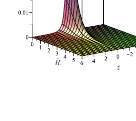
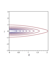
(a)	(b)
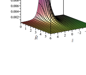
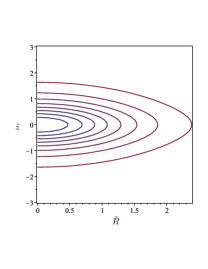
(c)	(d)
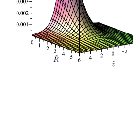
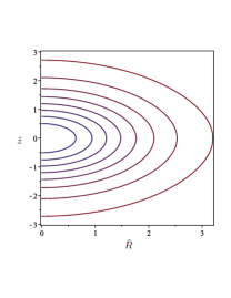
(e)	(f)

Figure 4: The relativistic energy density $\tilde{\rho}$ and the isodensity curves for the second family of Miyamoto-Nagai thick disk with parameters $\tilde{a}=1$ and $\tilde{b}=0.5$ (top figures), $1$ (middle figures), $2$ (bottom figures).

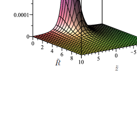
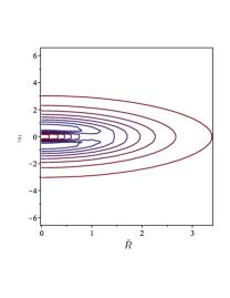
(a)	(b)
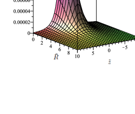
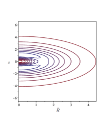
(c)	(d)
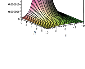
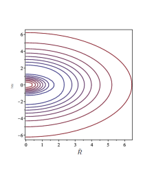
(e)	(f)

Figure 5: The relativistic average pressure $\tilde{p}$ and level curves for the second family of Miyamoto-Nagai thick disk with parameters $\tilde{a}=1$ and $\tilde{b}=0.5$ (top figures), $1$ (middle figures), $2$ (bottom figures).

In figures 4 and 5 we plot, as functions of $\tilde{R}$ and $\tilde{z}$, the relativistic energy density $\tilde{\rho}=G^{3}M^{2}\rho$, the average pressure $\tilde{p}=G^{3}M^{2}p$ and, in both cases, the level curves for the second model of Miyamoto-Nagai-like thick disks with parameters $\tilde{a}=1$, $\tilde{b}=0.5$ , $\tilde{b}=1$ and $\tilde{b}=2$. We observer that these functions present the same behavior as the previous model. However, since the gravitational potential (24a) (and hence the gravitational field) in absolute value is larger than the first model, these quantities have an order of magnitude higher in the second model.

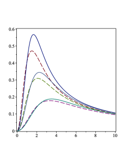
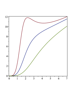
(a)	(b)

Figure 6: $(a)$ Relativistic and Newtonian rotation curves $v_{c}^{2}$ (solid curves) and $v_{N}^{2}$ (dashed curves) for the second model of Miyamoto-Nagai-like thick disks with parameters $\tilde{a}=1$, $\tilde{b}=0.5$ (top curves), $\tilde{b}=1$ and $\tilde{b}=2$ (bottom curves), as function of $\tilde{R}$. $(b)$ The specific angular momentum $\tilde{h}^{2}$ with parameters $\tilde{a}=1$, $\tilde{b}=0.5$ (top curve), $\tilde{b}=1$ and $\tilde{b}=2$ (bottom curve), also as function of $\tilde{R}$.

In figure 6 $(a)$ we depict, as function of $\tilde{R}$, the relativistic and Newtonian rotation curves $v_{c}^{2}$ and $v_{N}^{2}$ for the second family of Miyamoto-Nagai-like thick disks for the same value of the parameters. These quantities also show the same behavior as the first model. However, one find that the relativistic effects are more significant in the second model and moreover they have a higher value because the presence of a stronger gravitational field. Also here, the speed of the particles always is less than light speed (dominant energy condition). In figure 6 $(b)$ we show the specific angular momentum $\tilde{h}^{2}$ for the same values of parameters, also as function or $\tilde{R}$. Unlike the first model, the orbits of the particles can present regions of instability against radial perturbation when the structures are flatted (curve $\tilde{b}=0.5$).

V A relativistic model of galaxy

In Newtonian gravity, the Galactic potential is usually modeled by the sum of three components: a central spherical bulge $\Phi_{B}$, a thick disk $\Phi_{D}$ and a spherical dark halo $\Phi_{H}$, that is

$$\Phi=\Phi_{B}+\Phi_{D}+\Phi_{H}.$$ (28)

The bulge and disk potentials are represented in the form proposed by Miyamoto and Nagai

$$\Phi_{B} = -\frac{GM_{B}}{\sqrt{r^{2}+b_{B}^{2}}},$$ (29a)

$$\Phi_{D} = -\frac{GM_{D}}{\sqrt{R^{2}+\left(a_{D}+\sqrt{z^{2}+b_{D}^{2}}\right)^{2}}},$$ (29b)

where $r=\sqrt{R^{2}+z^{2}}$, and to describe the matter dark halo the potential is assumed to be the NFW model

$$\Phi_{H}=-\frac{GM_{H}}{r}\ln\left(1+\frac{r}{a_{H}}\right),$$ (30)

where $M_{H}$ is the dark halo mass and $a_{H}$ a scale radius. This potential satisfies our requirement that at large $R$ the metric function $\phi\ll 1$.

Since the Poisson’s equation is linear, the total mass density is the sum of the components

$$\rho_{N}=\rho_{N(B)}+\rho_{N(D)}+\rho_{N(H)}.$$ (31)

For the above potentials we have

$$\rho_{N(B)} = \frac{3b_{B}^{2}M_{B}}{4\pi(r^{2}+b_{B}^{2})^{5/2}},$$ (32a)

$$\rho_{N(D)} = \frac{b_{D}^{2}M_{D}\left[a_{D}R^{2}+(a_{D}+3\sqrt{z^{2}+b_{D}^{2}})(a_{D}+\sqrt{z^{2}+b_{D}^{2}})^{2}\right]}{4\pi\left[R^{2}+\left(a_{D}+\sqrt{z^{2}+b_{D}^{2}}\right)^{2}\right]^{5/2}(z^{2}+b_{D}^{2})^{3/2}},$$ (32b)

$$\rho_{N(H)} = \frac{M_{H}}{4\pi}\frac{1}{r(r+a_{H})^{2}}.$$ (32c)

From (17) it follows that the total circular speed is also the sum of the different contributions

$$v^{2}_{N}=v^{2}_{N(B)}+v^{2}_{N(D)}+v^{2}_{N(H)}.$$ (33)

For the above potentials we have

$$v_{N(B)}^{2} = \frac{GM_{B}R^{2}}{\left(R^{2}+b_{B}^{2}\right)^{3/2}},$$ (34a)

$$v_{N(D)}^{2} = \frac{GM_{D}R^{2}}{\left[R^{2}+(a_{D}+b_{D})^{2}\right]^{3/2}},$$ (34b)

$$v_{N(H)}^{2} = v_{0}^{2}\left[\frac{\ln(1+R/a_{H})}{R/a_{H}}-\frac{1}{1+R/a_{H}}\right],$$ (34c)

where $v_{0}^{2}=GM_{H}/a_{H}$.

Thus, the total relativistic circular speed is given by the non-linear expression

$$v_{c}^{2}=\frac{v^{2}_{N(B)}+v^{2}_{N(D)}+v^{2}_{N(H)}}{1-\frac{1}{2}(\Phi_{B}+\Phi_{D}+\Phi_{H})-v^{2}_{N(B)}-v^{2}_{N(D)}-v^{2}_{N(H)}}.$$ (35)

In order to analyze total relativistic tangential velocity $v_{c}$ and the different components we perform a graphical analysis of them for the values of the potential parameters computed in reference Bajkova $a_{D}=4.4$, $a_{H}=7.7$, $b_{B}=0.2672$, $b_{D}=0.3084$, $M_{b}=443$, $M_{d}=2798$ and $M_{h}=12474$. In figure 7 we graph, as function of $\tilde{R}=R/GM_{D}$, the relativistic and Newtonian total rotation curves $v_{c}$ and $v_{N}$ and the relativistic contributions of the three components: the central bulge $v_{B}$, the disk $v_{D}$ and the dark matter halo $v_{H}$. We see that total rotation curves are flatted after certain value of $\tilde{R}$ as the observational data reveal, whereas tangential speed of the visible matter (central bulge plus thick disk ) rapidly falls to zero. We find that the relativistic effects decrease the total tangential velocity everywhere and are more significant in the region close to its maximum value and, as expected, for velocities comparable to the speed of light (relativistic particles). In fact, the tangential velocity of the stars around a typical galaxy is about 200 - 300 km/s and therefore the relativistic effects are expected to be small. In the case of our Galaxy for a radius of $R=0.4$ kpc which corresponds to a tangential velocity about $260.8$ km/s we find that the relativistic corrections are of the order of $1.2\times 10^{-4}$ km/s. However, we believe that for a sufficiently large distance traveled by a star they could become important.

VI Discussion

Three-dimensional axisymmetric relativistic sources for a Majumdar-Papapetrou type conformastatic spacetime were construct from Newtonian potential-density pairs. As simple examples, were considered two family of Miyamoto-Nagai-like thick disk models and a relativistic model of galaxy composite by three components: a central bulge, a disk and a NFW dark matter halo.

The equatorial circular motion of test particles around such configurations were studied, and in all models was observed that the relativistic effect are more important in the regions around its maximum value and, as expected, for velocities comparable to the speed of light. In the case of the thick disks was found that such effects initially decrease the circular speed of the particles and just before reaching its maximum value, they increase it, whereas for the relativistic model of galaxy presented the relativistic effects always decrease the circular speed. Also was observed that the relativistic corrections are more significant in the second disk model. Moreover, all the physical quantities computed have an order of magnitude higher in the second model due to the presence of a stronger gravitational field.

The stability of the orbits for radial perturbation was analyzed for the thick disks using an extension of the Rayleigh criterion. We found values of parameters for which the motion of particles is stable against radial perturbation. The models constructed satisfying all the energy conditions.

References

$$\begin{array}[]{cc}\includegraphics[width=143.09538pt]{ener1.eps}&\includegraphics[width=108.405pt]{contor1.eps}\\ &\\ (a)&(b)\\ \includegraphics[width=143.09538pt]{ener2.eps}&\includegraphics[width=108.405pt]{contor2.eps}\\ &\\ (c)&(d)\\ \includegraphics[width=143.09538pt]{ener3.eps}&\includegraphics[width=108.405pt]{contor3.eps}\\ &\\ (e)&(f)\end{array}$$

Figure 1: The relativistic energy density $\tilde{\rho}$ and the isodensity curves for the first model of Miyamoto-Nagai-like thick disks with parameters $\tilde{a}=1$ and $\tilde{b}=0.5$ (top figures), $1$ (middle figures), $2$ (bottom figures).

$$\begin{array}[]{cc}\includegraphics[width=143.09538pt]{pr1.eps}&\includegraphics[width=108.405pt]{contorpr1.eps}\\ &\\ (a)&(b)\\ \includegraphics[width=143.09538pt]{pr2.eps}&\includegraphics[width=108.405pt]{contorpr2.eps}\\ &\\ (c)&(d)\\ \includegraphics[width=143.09538pt]{pr3.eps}&\includegraphics[width=108.405pt]{contorpr3.eps}\\ &\\ (e)&(f)\end{array}$$

Figure 2: The relativistic average pressure $\tilde{p}$ and the level curves for the first model of Miyamoto-Nagai-like thick disks with parameters $\tilde{a}=1$ and $\tilde{b}=0.5$ (top figures), $1$ (middle figures), $2$ (bottom figures).

$$\begin{array}[]{cc}\includegraphics[width=130.08731pt]{v2mn1.eps}&\includegraphics[width=130.08731pt]{h2mn1.eps}\\ \tilde{R}&\tilde{R}\\ &\\ (a)&(b)\end{array}$$

Figure 3: $(a)$ Relativistic and Newtonian rotation curves $v_{c}^{2}$ (solid curves) and $v_{N}^{2}$ (dashed curves) for the first model of Miyamoto-Nagai-like thick disks with parameters $\tilde{a}=1$, $\tilde{b}=0.5$ (top curves), $\tilde{b}=1$ and $\tilde{b}=2$ (bottom curves), as function of $\tilde{R}$. $(b)$ The specific angular momentun $\tilde{h}^{2}$ with parameters $\tilde{a}=1$, $\tilde{b}=0.5$ (top curve), $\tilde{b}=1$ and $\tilde{b}=2$ (bottom curve), also as function of $\tilde{R}$.

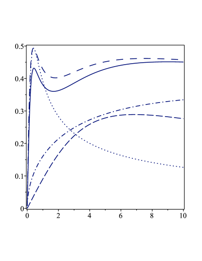
$\tilde{R}$

Figure 7: Relativistic and Newtonian total rotation curves $v_{c}$ (solid curve) and $v_{N}$ (top curve) and the relativistic contributions of the three components: central bulge $v_{B}$ (dotted curve), disk $v_{D}$ (dashed curve) and dark halo $v_{H}$ (dash-dotted curve), as function of $\tilde{R}$.

References

- (1) G. G. Kuzmin 1956, Astron. Zh. 33, 27 (1956).
- (2) A. Toomre, Ap. J. 138, 385 (1962).
- (3) M. Miyamoto and R. Nagai, PASJ 27, 533 (1975).
- (4) R. Nagai and M. Miyamoto, PASJ 28, 1 (1976).
- (5) H. C. Plummer, MNRAS 71, 460 (1911).
- (6) C. Allen and A. Santillan, Rev. Mexicana Astron. Astrof. 22, 255 (1991).
- (7) S. Ninkovic, Rev. Mexicana Astron. Astrof. 53, 113 (2017).
- (8) A. T. Bajkova and V. V. Bobylev, Astronomy Letters 42, No. 9, 567 (2016).
- (9) S. Ninkovic, PASA 32, e032, (2015).
- (10) J. Binney and S. Tremaine S, 2008, Galactic Dynamics, 2nd edn. Princeton Univ. Press, Princeton, NJ.
- (11) W. A. Bonnor and A. Sackfield, Commun. Math. Phys. 8, 338 (1968).
- (12) T. Morgan and L. Morgan, Phys. Rev. 183, 1097 (1969).
- (13) L. Morgan and T. Morgan, Phys. Rev. D 2, 2756 (1970).
- (14) D. Lynden-Bell and S. Pineault, Mon. Not. R. Astron. Soc. 185, 679 (1978).
- (15) A. Chamorro, R. Gregory, and J. M. Stewart, Proc. R. Soc. London A413, 251 (1987).
- (16) P.S. Letelier and S. R. Oliveira, J. Math. Phys. 28, 165 (1987).
- (17) J. P. S. Lemos, Class. Quantum Grav. 6, 1219 (1989).
- (18) J. Bic̆ák, D. Lynden-Bell, and J. Katz, Phys. Rev. D 47, 4334 (1993).
- (19) J. Bic̆ák, D. Lynden-Bell, and C. Pichon, Mon. Not. R. Astron. Soc. 265, 126 (1993).
- (20) G. A. González and O. A. Espitia, Phys. Rev. D 68, 104028 (2003).
- (21) J. Bic̆ák and T. Ledvinka, Phys. Rev. Lett. 71, 1669 (1993).
- (22) G. A. González and P. S. Letelier, Phys. Rev. D 62, 064025 (2000).
- (23) J. P. S. Lemos and P. S. Letelier, Class. Quantum Grav. 10, L75 (1993).
- (24) J. P. S. Lemos and P. S. Letelier, Phys. Rev. D 49, 5135 (1994).
- (25) G. A. González and P. S. Letelier, Phys. Rev. D 69, 044013 (2004).
- (26) D. Vogt and P. S. Letelier, MNRAS 363, 268 ( 2005).
- (27) G. García-Reyes, Gen. Relativ. Gravit. 49, 3, 1 (2017).
- (28) J. F. Navarro, C. S. Frenk and S. D. M. White, Ap. J. 462, 563 (1996).
- (29) Lord Rayleigh, 1917, Proc. R. Soc. London A, 93, 148
- (30) L. D. Landau and E. M. Lifshitz, Fluid Mechanics(Addison-Wesley, Reading, MA, 1989).
- (31) J. L. Synge, Relativity: The General Theory (North- Holland, Amsterdam, 1966).
- (32) H. Stephani, D. Kramer, M. McCallum, C. Hoenselaers, and E. Herlt, Exact Solutions of Einsteins’s Field Equations (Cambridge University Press, Cambridge, England, 2003).
- (33) S. D. Majumdar, Phys. Rev. 72, 390 (1947).
- (34) A. Papapetrou , Proc. Roy. Soc. (London) A51, 191 (1947).