Temperature Dependence of Nonlinear Susceptibilities in an Infinite Range Interaction Model

Abstract

We present a model to probe metamagnetic properties in systems with an arbitrary number of interacting spins. Thermodynamic properties such as the magnetization per particle $m(B,T,N)$, linear susceptibility $\chi_{1}(T)$, and nonlinear susceptibilities $\chi_{3}(T)$ and $\chi_{5}(T)$ were calculated. The model produces a different magnetic response for $N$ particles when comparing to $N-1$ particles for small $N\sim 1$. For an even number of particles, the susceptibilities show maxima in their temperature dependence. An odd number produces an additional free spin response that dominates at low temperatures. This free spin response also produces a step in the magnetization per particle at $B=0$ for odd $N$. The magnetization shows $N/2$ steps at $\gamma B_{c}/J=n$ with integer $n$ for even $N$ and $(N-1)/2$ additional steps at with integer $n$ for odd $N$. Small clusters respond with metamagnetism in an otherwise isotropic spin space, while the large clusters show no metamagnetism.

I 1. Introduction

Metamagnetism Stryjewski:77 ; Levitin:88 ; Goto:01 is identified as when the magnetization rapidly rises at a critical magnetic field. Typically this happens at low temperatures and the critical field is nearly insensitive to the temperature. The transition broadens with increased temperature. In a transition metal antiferromagnet, the transition is described Stryjewski:77 as a first order spin flop transition. When the magnetic field is applied along some unpreferred direction, the low field response is weak because the spins are locked along the preferred direction. The spins line up along the magnetic field when the field exceeds the anisotropy energy.

It was proposed wohlfarth:62 ; Aoki:13 that for metals a first order phase transition occurs. When considering an expansion of the Ginzburg Landau free energy in terms of the magnetization, this transition is caused by a negative fourth order term due to the density of states of the material. The metal would then have a metamagnetic phase transition similar to a liquid-gas phase transition.

Many materials Rost:09 ; Thomas:16 show a sharp metamagnetism only at $T=0$, contrary to the Wohlfarth-Rhodes narrative. With a $T>0$, the transition is no longer discontinuous and smoothly disappears. This is consistent with a quantum phase transition Millis:02 ; DHoker:10 , thermodynamically analogous to the ferromagnetic transition. Where the ferromagnetic transition occurs at $B=0$ and $T=T_{c}$, the metamagnetic transition occurs at $B=B_{c}$ and $T=0$.

Metamagnetism in an insulating antiferromagnet is easily discussed in terms of an anisotropic exchange Hamiltonian. The anisotropy derives from crystalline electric fields and depends on the field orientation with respect to the lattice structure. In a metal such as the heavy fermions, the sensitivity to the lattice structure is less clear in experiments. However, a discrete level structure whose crossing represents the metamagnetism should be describable in terms of a spin Hamiltonian. We therefore pick an example (see another example in Ref. Bak:82 ) and study its consequences.

The recent study Shivaram:14 by Shivaram et al., starting with the measurement of metamagnetism for heavy fermion compounds, notes certain correlations between the observables. It was already noted by Goto et al. Goto:01 that the linear susceptibility showed a peak at a temperature $T_{1}$ and that the critical field $B_{c}$ scaled with the inverse susceptibility at that maximum. Hirose et al. Hirose:11 pointed out that critical field followed the susceptibility peak temperature. Shivaram et al. also noted the correlation in the peak temperatures of the nonlinear susceptibilities. They seemed to favor a single energy scale in these phenomena. Thermodynamics connects the temperature dependence of magnetization to the field dependence of the specific heat or the sound velocity. Here, we find similar results for an otherwise general Hamiltonian. The series of compounds CeMIn₅ show a Curie law susceptibility at low temperatures as reported by Thamizhavel et al. Thamizhavel:15 . B. Shivaram Shivaram:15 has noted several instances of metamagnetism in different contexts. For a review of molecular magnets see also Ref. Schnack:13 .

This paper presents an overview of a model describing a cluster of $N$ fermionic (spin $s=1/2$) spins interacting through an infinite range antiferromagnetic interaction $J$. These interacting spins are influenced by an external magnetic field $B$ in the direction of the spin quantization axis $z$. The model is meant to solely study the spin contribution to metamagnetism. Using the dimensionless variables $\tau=k_{B}T/J$ and $b=\gamma B/J$, the principal results are summarized here:

1. The responses for even and odd number of particles are qualitatively different. There are $(N+n_{0})/2$ steps in the magnetization with $n_{0}=N\mod 2$ describing the “oddness” of $N$ (for even $N$, $n_{0}=0$ and for odd $N$, $n_{0}=1$). The steps occur at critical field values

   $$B_{c}=\left(\frac{2n+n_{0}}{2}\right)\frac{J}{\gamma}\quad\quad n=1,2,...,\frac{N-n_{0}}{2}$$

   The magnetization per particle changes by $1/N$ at each $B_{c}$. When $N$ is odd, there is an additional step at $B_{c}=0$ due to a free spin response which changes the magnetization per particle by $1/2N$. The fully saturated magnetization per particle is $m=1/2$ for all $N$.

2. For odd $N$, the ground state is a Kramer’s doublet leading to a free spin response (see discussion after Eq. 3.1 in Ref. Alcaraz:88 ); a Curie law contribution to the total susceptibility.

3. The nonlinear susceptibilities are defined as

   $$M=\chi_{1}(T)B+\chi_{3}(T)B^{3}+\chi_{5}(T)B^{5}.$$

   The third and fifth order susceptibilities are negative at high temperatures. The susceptibilities rise at low temperatures and show a maximum at a characteristic temperature. For even $N$, they all go to zero at $T=0$. For odd $N$, there is a free spin response which dominates at low temperatures. Shivaram et al. Shivaram:14 studied another basic Hamiltonian $H=\Delta S_{z}^{2}-\gamma BS_{z}$ showing similar results.

4. The specific heat as a function of temperature at $b=0$ is Schottky-like. It rises exponentially at low temperatures and decays as $\tau^{-2}$ at high temperatures. As a function of magnetic field at low temperatures, the specific heat has a minimum at the critical fields buttressed by peaks both below and above the critical field. As the temperature increases, the minima stay fixed but the peaks move out.

The rest of the paper is organized as follows: Sec. 2 focuses on the details of the infinite range exchange interaction model. The partition function and the observables are discussed for a generalized particle number $N$, commenting on the difference in the even $N$ and odd $N$ cases. Sec. 3 presents the results in the small $N$ limit ($N=2,3$), and Sec. 4 discusses the large $N$ limit ($N=23,24$) and the thermodynamic limit ($N\rightarrow\infty$). Sec. 5 contains a summary of the results and a discussion of the limitations of the model.

II 2. Model

In the model considered here, each spin interacts with all other spins. The Hamiltonian is

$$H=J\sum_{i<j}\mathbf{s}_{i}\cdot\mathbf{s}_{j}-\gamma\mathbf{B}\cdot\mathbf{S}.$$ (1)

Here $J$ is an antiferromangeitc exchange interaction of infinite range, $\gamma$ is the gyromagnetic ratio, $B$ is the external field, and $\mathbf{S}=\sum_{i}\mathbf{s}_{i}$ is the total spin of the system. The eigenenergies of the system are calculated using the identity:

$$2\sum_{i<j}\mathbf{s}_{i}\cdot\mathbf{s}_{j}=\left(\sum_{i}\mathbf{s}_{i}\right)^{2}-\sum_{i}s_{i}^{2}=S^{2}-\frac{3}{4}N.$$ (2)

This produces the eigenenergies

$$\lambda=\frac{J}{2}S(S+1)-\frac{3N}{8}J-\gamma B\mu,$$ (3)

where $\mu$ is the $z$ component of spin and $S$ is the quantized spin eigenvalue. The range of values for $\mu$ and $S$ depend on whether there are an even or odd number of particles. For generalization, it is useful to define the variable $n_{0}=N\mod 2$, same as above. The range of values for $\mu$ and $S$ can then be written $-S\leq\mu\leq S$ and $\frac{1}{2}n_{0}\leq S\leq N/2$, with all values spaced by an integer. The partition function can then be written from these eigenenergies

$$Z=e^{3JN/8}\sum_{S=\frac{1}{2}n_{0}}^{N/2}e^{-S(S+1)/2\tau}\sum_{\mu=-S}^{S}e^{\mu b/\tau}.$$ (4)

Here $\tau=k_{B}T/J$ and $b=\gamma B/J$ are dimensionless variables describing the temperature and field. The prefactor $\exp(3JN/8)$ is a constant multiple that will cancel when calculating thermal properties, and will thus be dropped from here on. Finally the partition function leads to the Gibbs’ free energy such that $F=-k_{B}T\ln Z$, from which comes the thermodynamic properties: magnetization $M=-\frac{\partial F}{\partial B}$, specific heat $C=-T\frac{\partial^{2}F}{\partial T^{2}}$ and pressure $P=-\frac{\partial F}{\partial V}$. For the pressure there is no explicit volume dependence. The results in this paper assume a volume dependence on the coupling strength $J(V)=gV$ leading to the pressure $P=-\left(\frac{\partial J}{\partial V}\right)\frac{\partial F}{\partial J}=-g\frac{\partial F}{\partial J}$. For simplicity all discussion of pressure is in units of $g$.

To more easily evaluate the thermodynamic properties, the partition function can be rewritten by changing the order of the summations. To simplify the expression, the field-independent function $A_{\mu}(N)=\sum_{S=\mu}^{N/2}e^{-S(S+1)/2\tau}$ is used. The even and odd partition functions are then,

$$Z(N=2n) =A_{0}(N)+2\sum_{\mu=1}^{N/2}A_{\mu}(N)\cosh\left(\frac{\mu b}{\tau}\right),$$

$$Z(N=2n+1) =2\sum_{\mu=1/2}^{N/2}A_{\mu}(N)\cosh\left(\frac{\mu b}{\tau}\right).$$ (5)

From here the magnetization $M$ for each becomes,

$$\frac{M(N=2n)}{\gamma} =\frac{2\sum_{\mu=1}^{N/2}\mu A_{\mu}(N)\sinh(\mu b/\tau)}{A_{0}(N)+2\sum_{\mu=1}^{N/2}A_{\mu}(N)\cosh(\mu b/\tau)},$$

$$\frac{M(N=2n+1)}{\gamma} =\frac{\sum_{\mu=1/2}^{N/2}\mu A_{\mu}(N)\sinh(\mu b/\tau)}{\sum_{\mu=1/2}^{N/2}A_{\mu}(N)\cosh(\mu b/\tau)}.$$ (6)

The nonlinear susceptibilities follow from these expressions. Likewise the other thermodynamic observables such as specific heat or pressure (the field dependent part, using the implicit volume dependence of $J$) can be obtained using the other thermodynamic derivatives.

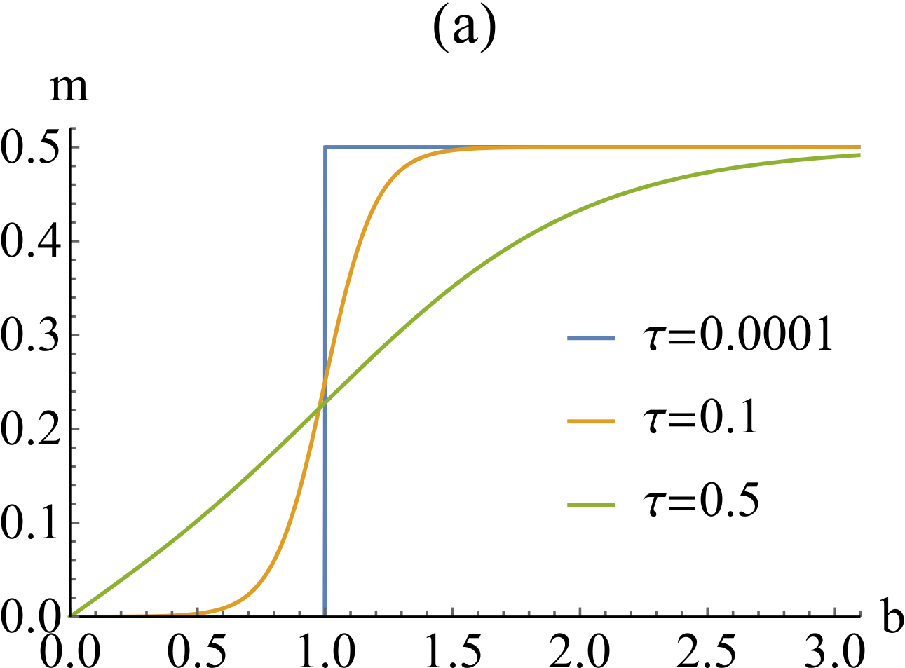
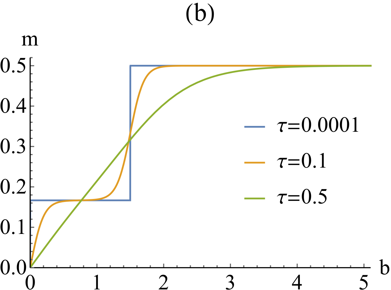
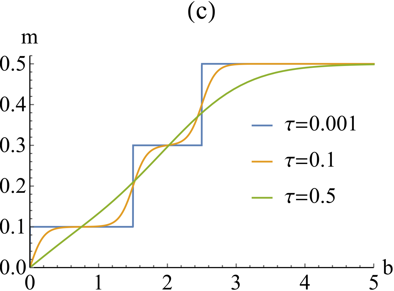
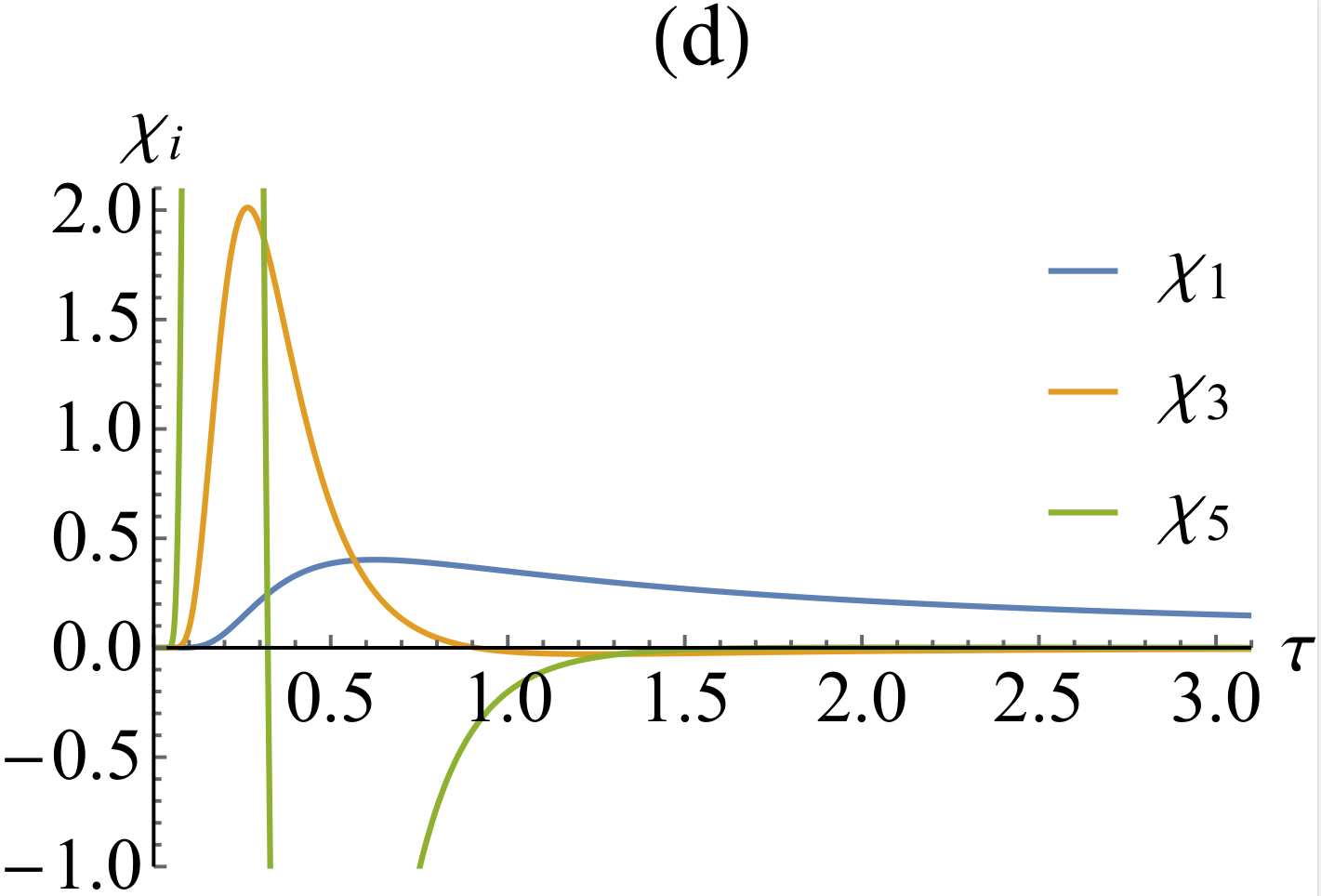
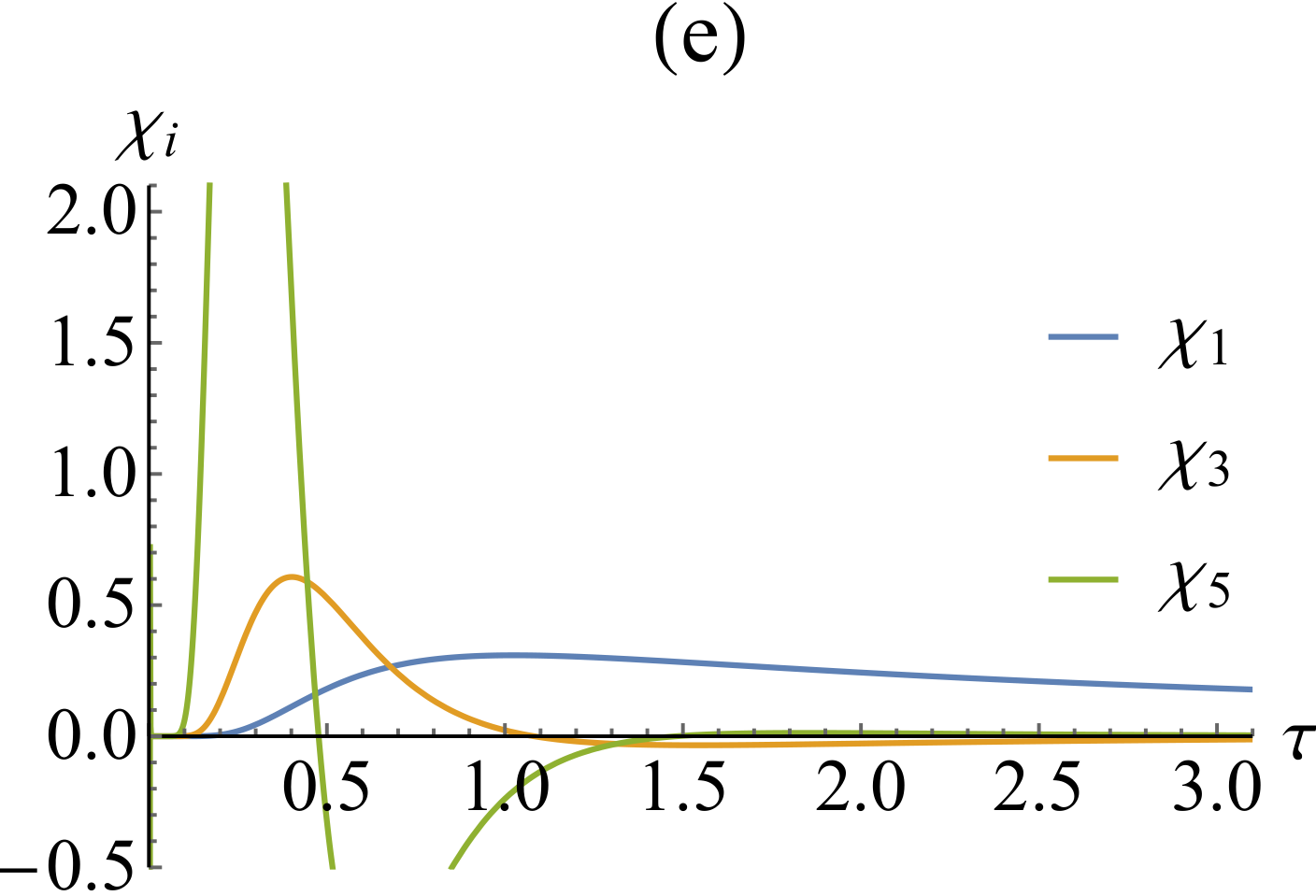
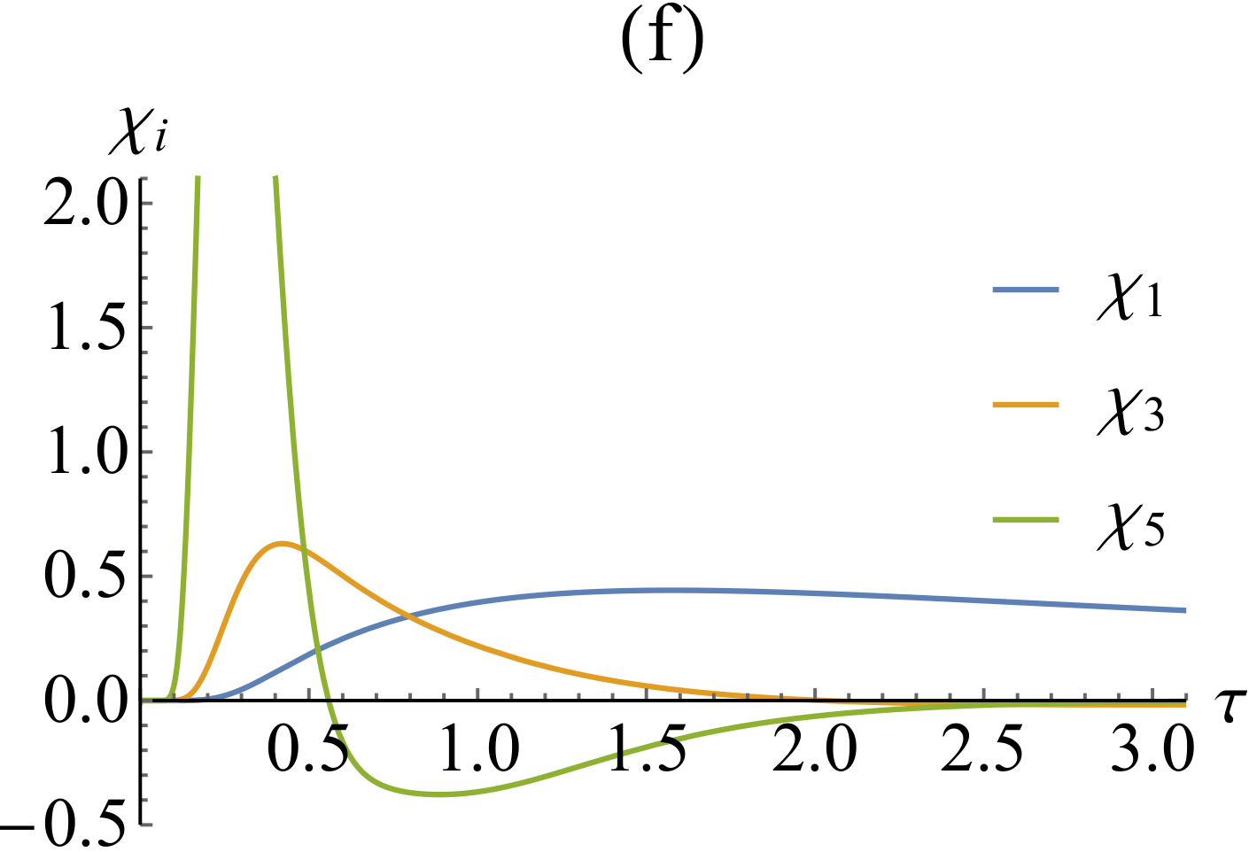
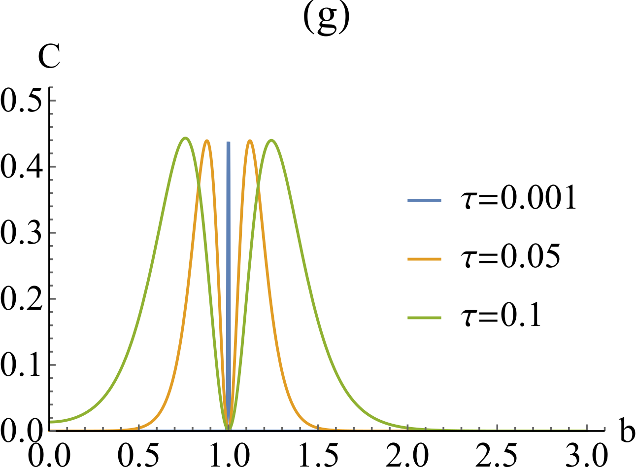
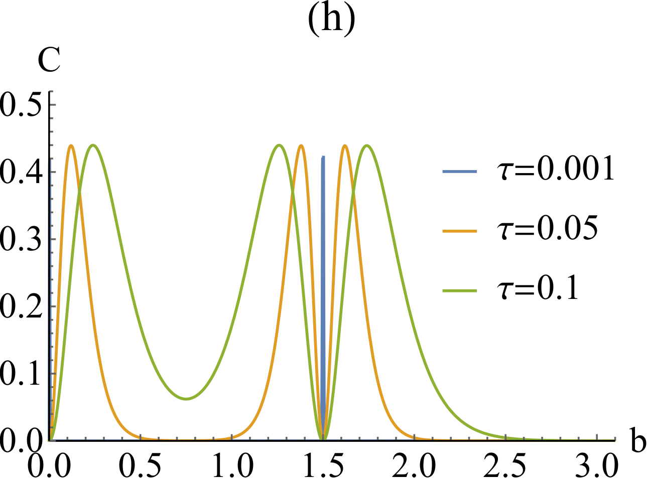
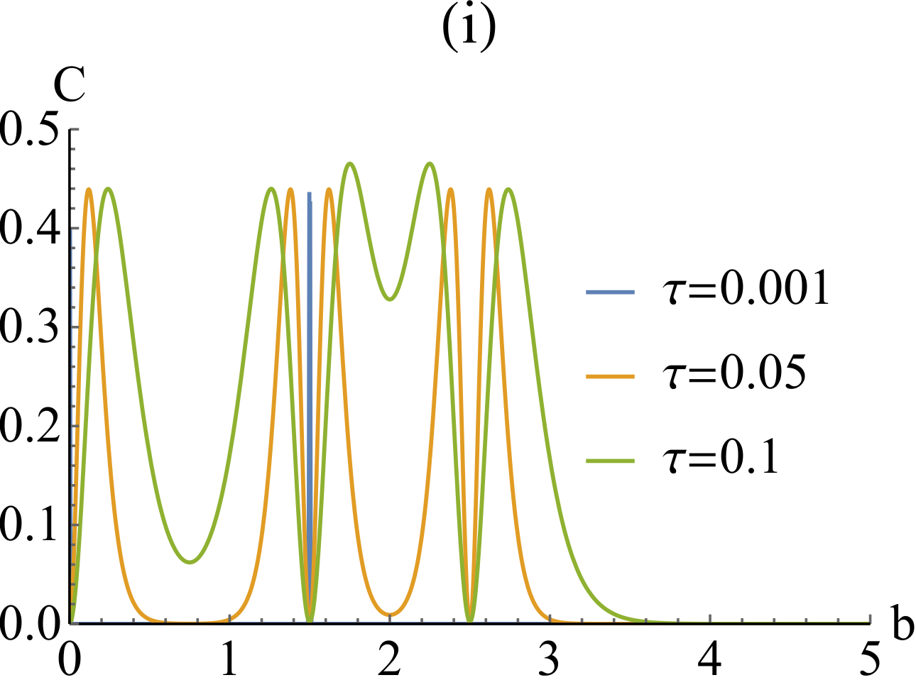
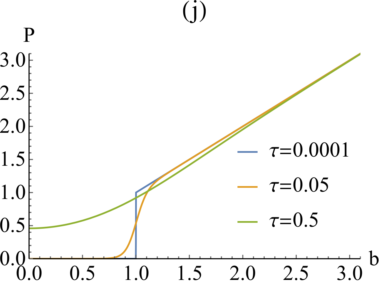
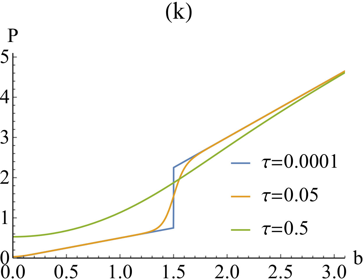
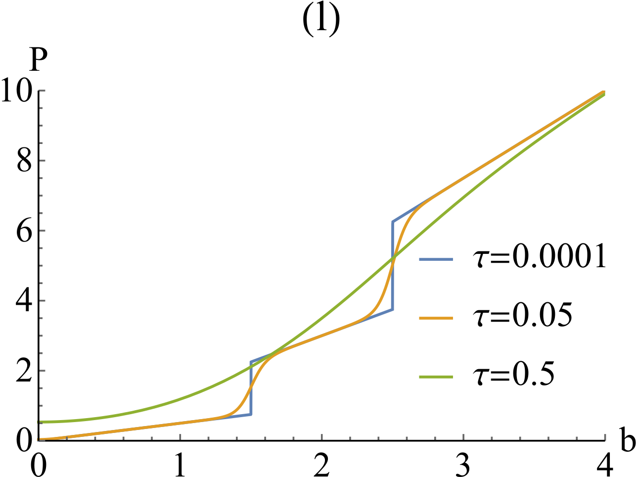
Figure 1: Thermodynamic quantities for $N=2,3,5$ particles. (a),(d),(g),(j) are for $N=2$, (b),(e),(h),(k) for $N=3$, and (c),(f),(i),(l) for $N=5$. The first row ((a)-(c)) shows the magnetization per particle $m$ vs. field $b$ for three temperatures $\tau=0.0001,0.1,0.5$. The second row ((d)-(f)) shows the linear susceptibility $\chi_{1}$ and the first two nonlinear susceptibilities $\chi_{3},\chi_{5}$ vs. temperature $\tau$. Both (e) and (f) have subtracted out the free spin response contribution to the susceptibilities. The third row ((g)-(i)) shows the specific heat $C$ vs. field $b$ for three temperatures $\tau=0.001,0.05,0.1$. The final row ((j)-(l)) shows the pressure $P$ vs. field $b$ for three temperatures $\tau=0.0001,0.05,0.5$.

It is possible to rewrite the magnetization for odd particle number $M(N=2n+1)$ in order to highlight the free spin term. This calculation gives a term similar to what is seen for $M(N=2n)$ in Eq. (6),

$$\frac{M(N=2n+1)}{\gamma}=\frac{1}{2}\tanh\left(\frac{b}{2\tau}\right)+\frac{2\sum_{\mu=3/2}^{N/2}(\mu-1/2)B_{\mu}(N)\sinh((\mu-1/2)b/\tau)}{B_{1/2}(N)+2\sum_{\mu=3/2}^{N/2}B_{\mu}(N)\cosh((\mu-1/2)b/\tau)},$$ (7)

where $B_{\mu}(N)$ is defined from the functions $A_{m}(N)$,

$$B_{\mu}(N)=2\sum_{m=\mu}^{N/2}(-1)^{m-\mu}A_{m}(N).$$ (8)

By reindexing the sums in Eq. (7) using $\mu^{\prime}=\mu-1/2$ and replacing $B_{\mu^{\prime}+1/2}(N)$ with $A_{\mu^{\prime}}(N-1)$ the second term gives back the magnetization for even particle number. The full derivation of the above equivalency can be seen in Appendix A.

III 3. Small $N$ Limit

At this stage it is important to look into expressions for specific values of $N$, both to get a better, more comprehensive understanding and also to check the validity of some results in the space of hyperbolic functions. Some of these results can be derived by direct calculation of the partition function and used as a check.

(a) $N=2:$

Two spin half particles are described by a partition function $Z=1+e^{-1/\tau}(1+2\cosh b/\tau)$. The magnetization $M$ is given by

$$M=\gamma\frac{\sinh(b/\tau)}{C_{2}+\cosh(b/\tau)},\quad\quad C_{2}=\frac{1}{2}A_{0}(2)=\frac{1}{2}(1+e^{1/\tau}).$$ (9)

which leads to

$$\chi_{1}(T) =\frac{\gamma^{2}}{kT}\frac{1}{1+C_{2}},$$ (10a)

$$\chi_{3}(T) =\frac{\gamma}{3!}\left(\frac{\gamma}{kT}\right)^{3}\frac{C_{2}-2}{(1+C_{2})^{2}},$$ (10b)

$$\chi_{5}(T) =\frac{\gamma}{5!}\left(\frac{\gamma}{kT}\right)^{5}\frac{C_{2}^{2}-13C_{2}+16}{(1+C_{2})^{3}}.$$ (10c)

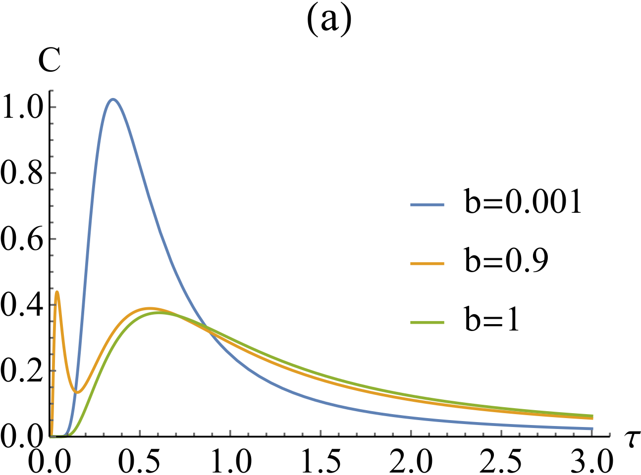
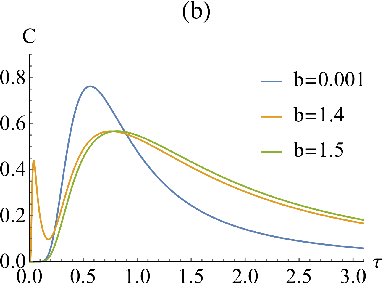
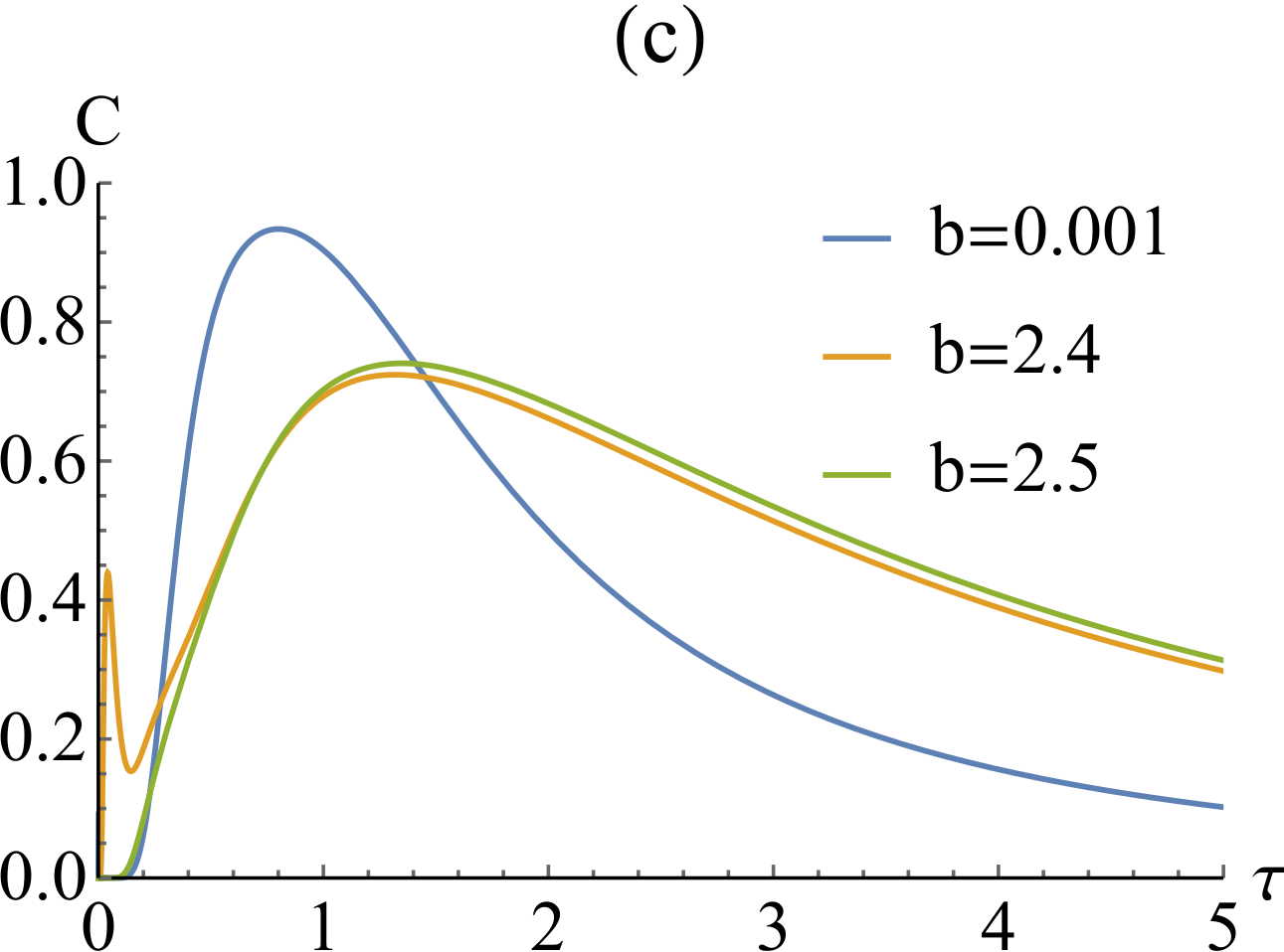
Figure 2: Specific heat versus temperature for $N=2,3,5$. (a) The specific heat for $N=2$ for field values $b=0.001,0.9,1$. These values show the change from small $b$ to the humps that occur at small $\tau$ for $b\sim b_{c}$. (b) The specific heat for $N=3$ for field values $b=0.001,1.4,1.5$. Humps form similarly to the $N=2$ case. (c) The specific heat for $N=5$ for field values $b=0.001,2.4,2.5$. These plots emphasize the humps occurring for small temperatures $\tau$ when $b\sim b_{c}$.

These are the principal nonlinear susceptibilities. The results for the linear susceptibility Bleaney:52 and zero temperature magnetization Tachiki:70 are well known. The results are shown in Figs. 1(d). The temperature dependence of the susceptibilities is qualitatively similar to the anisotropy based models Shivaram:14 (replacing $C_{2}\rightarrow\frac{1}{2}e^{1/\tau}$). The linear susceptibility $\chi_{1}$ has a maximum at $T_{1}=0.624J$ and vanishes at both low and high temperatures. At high temperatures, it has an effective Curie-Weiss temperature $\theta=J/4$. The third order susceptibility $\chi_{3}(T)$ is negative at high temperatures but has a positive maximum at $T_{3}=0.265J$ and vanishes at $T=0$. The next order nonlinear susceptibility, $\chi_{5}(T)$ is qualitatively similar with a peak at $T_{5}=0.176J$.

The specific heat for $N=2$ is shown versus magnetic field in Fig. 1(g) and versus temperature in Fig. 2(a). As a function of temperature, the specific heat has the usual Schottky features, e.g. those of the specific heat of a two level system. They include an exponential rise at low $T$ and an inverse power law decay at high temperatures. As a function of magnetic field for low $T$ in Fig. 1(g), it has the $M$ shaped response centered at $b=1$. As the temperature increases, the specific heat at $b=0$ increases, the two peaks move away from each other, but the minimum stays around $b=1$.

The magnetic field dependent part of the pressure is shown in Fig. 1(j). It consists of a threshold proportional to temperature at $b=1$ and a linear dependence on $b$ for $b>1$.

(b) $N=3,5:$

Here the ground state is a Kramer’s doublet. This leads to several interesting effects. The partition function for $N=3$ is given by:

$$Z=2e^{-3/8\tau}\cosh\left(\frac{b}{2\tau}\right)\left[1+2e^{3/2\tau}\cosh\left(\frac{b}{\tau}\right)\right]$$ (11)

and the magnetization $M$ is given by

$$\begin{split}M&=\frac{\gamma}{2}\tanh\left(\frac{b}{2\tau}\right)+\gamma\frac{\sinh(b/\tau)}{C_{3}+\cosh(b/\tau)},\\ C_{3}&=\frac{1}{2}B_{1/2}(3)=\frac{1}{2}e^{3/2\tau}.\end{split}$$ (12)

The first term is the free particle $S=1/2$ response. With the odd number of particles this is the dominant contribution at low temperatures. The linear and nonlinear susceptibilities are given by

$$\chi_{1} =\frac{\gamma^{2}}{4kT}\left[1+\frac{4}{1+C_{3}}\right],$$ (13a)

$$\chi_{3} =\frac{\gamma}{3}\left(\frac{\gamma}{2kT}\right)^{3}\left[1+2^{3}\frac{C_{3}-2}{(1+C_{3})^{2}}\right],$$ (13b)

$$\chi_{5} =\frac{2\gamma}{15}\left(\frac{\gamma}{2kT}\right)^{5}\left[1+2^{5}\frac{5C_{3}^{2}-13C_{3}+16}{(1+C_{3})^{3}}\right].$$ (13c)

The first term in each of the above equations is the free particle $s=1/2$ response. The second term is (and the following terms are) the usual linear and nonlinear susceptibility albeit with an $N$ dependent $C_{N}$. There is a step at $b=0$ leading to a magnetization per particle $m=1/6$. This is followed by a step at $b=3/2$ with $m=1/2$. For odd number of particles without a magnetic field the ground state is doubly degenerate and the magnetization vanishes. However at the smallest field there is a separation in the energy levels for the $m=\pm 1/2$ leading to a nonzero magnetization at low $T$ and a step in $m(b)$ at $b=0$.

The general features for an odd $N$ are seen in Figs. 1 for both $N=3$ and $N=5$. The $N=5$ plots more clearly show these features. Figs. 1(b),(c) show the magnetization steps at the critical values of the magnetic field. The step at $b=0$ is followed by one at $b=3/2$ (for $N=3,5$) and at 5/2 (for $N=5$). Figs. 1(e),(f) show the linear and nonlinear susceptibilities with the low temperature limit with the free spin response contribution removed. When included, all $\chi_{i}$ are divergent for the $\tau\rightarrow 0$ limit. The features are similar to the even $N$ response characteristic of the model; negative at high $T$. As in the even $N$ case the specific heat (Figs. 1(h),(i)) dips to zero at the critical field values for small temperatures. The temperature dependence of the specific heat can be seen in Figs. 2(b),(c) for $N=3,5$. The pressure as a function of magnetic field (Figs. 1(k),(l)) show the phase transition at the critical field values, along with a slope equal to the ground state spin for small $\tau$.

IV 4. Large $N$ Limit

The partition function in Eq. (4) has a large $N$ limit which can be studied in two alternative ways. Analytically, an infinite $N$ limit can be studied by replacing the sum by an integral. The magnetization turns into a Gaussian integral of the form:

$$M=\int_{n_{0}/2}^{\infty}dSe^{-S(S+1)/2}f(S),\quad f(S)=\frac{\sinh\left(\frac{(2S+1)b}{2\tau}\right)}{\sinh(b/2\tau)},$$

which can be evaluated in terms of error functions. The results can be made more transparent by evaluating the sums directly over a large number of particles, such as $N=23$ or 24 (odd and even cases separately), and interpolating $N\rightarrow\infty$.

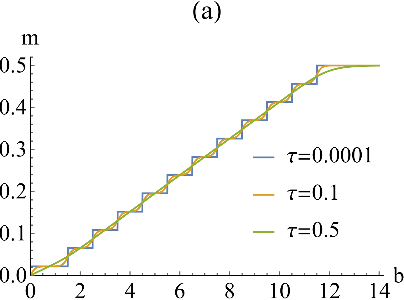
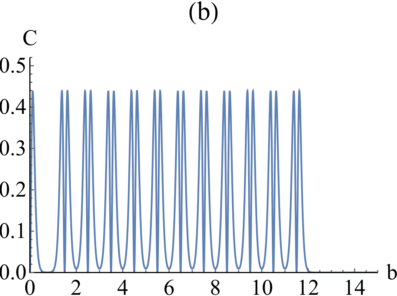
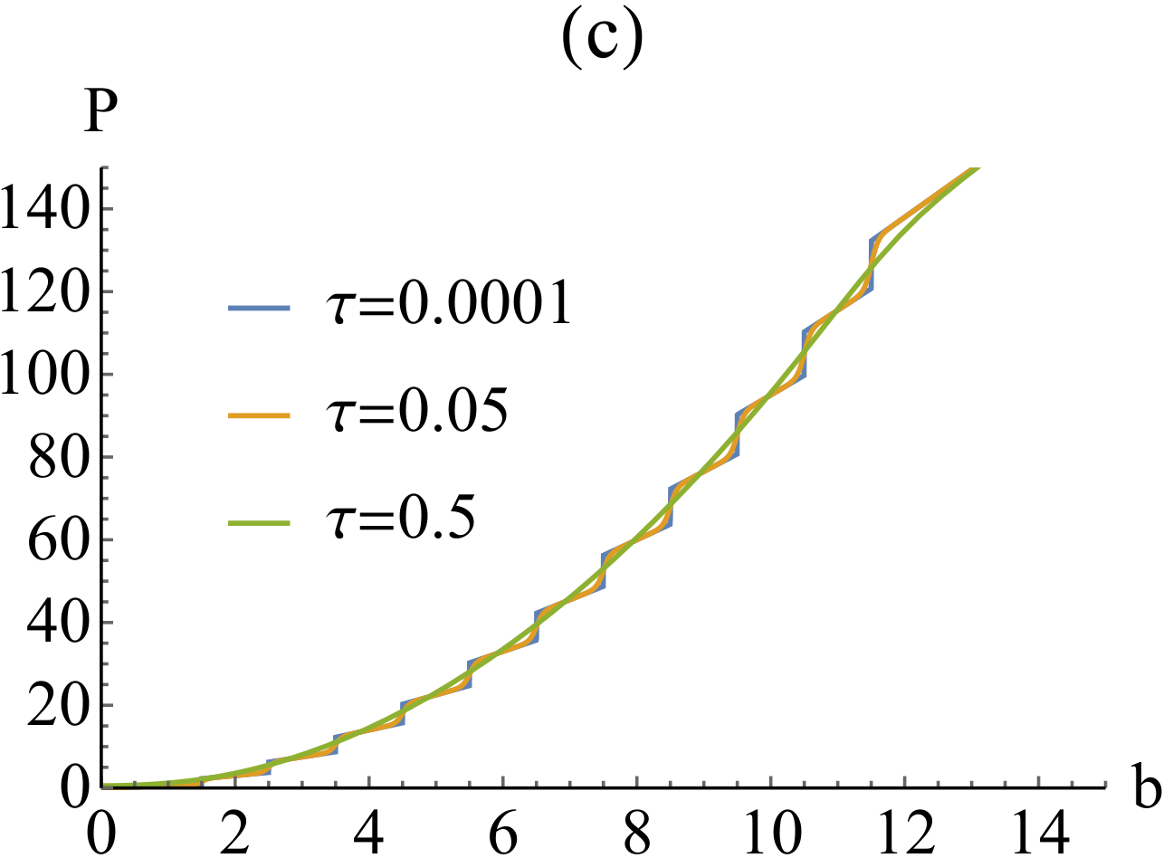
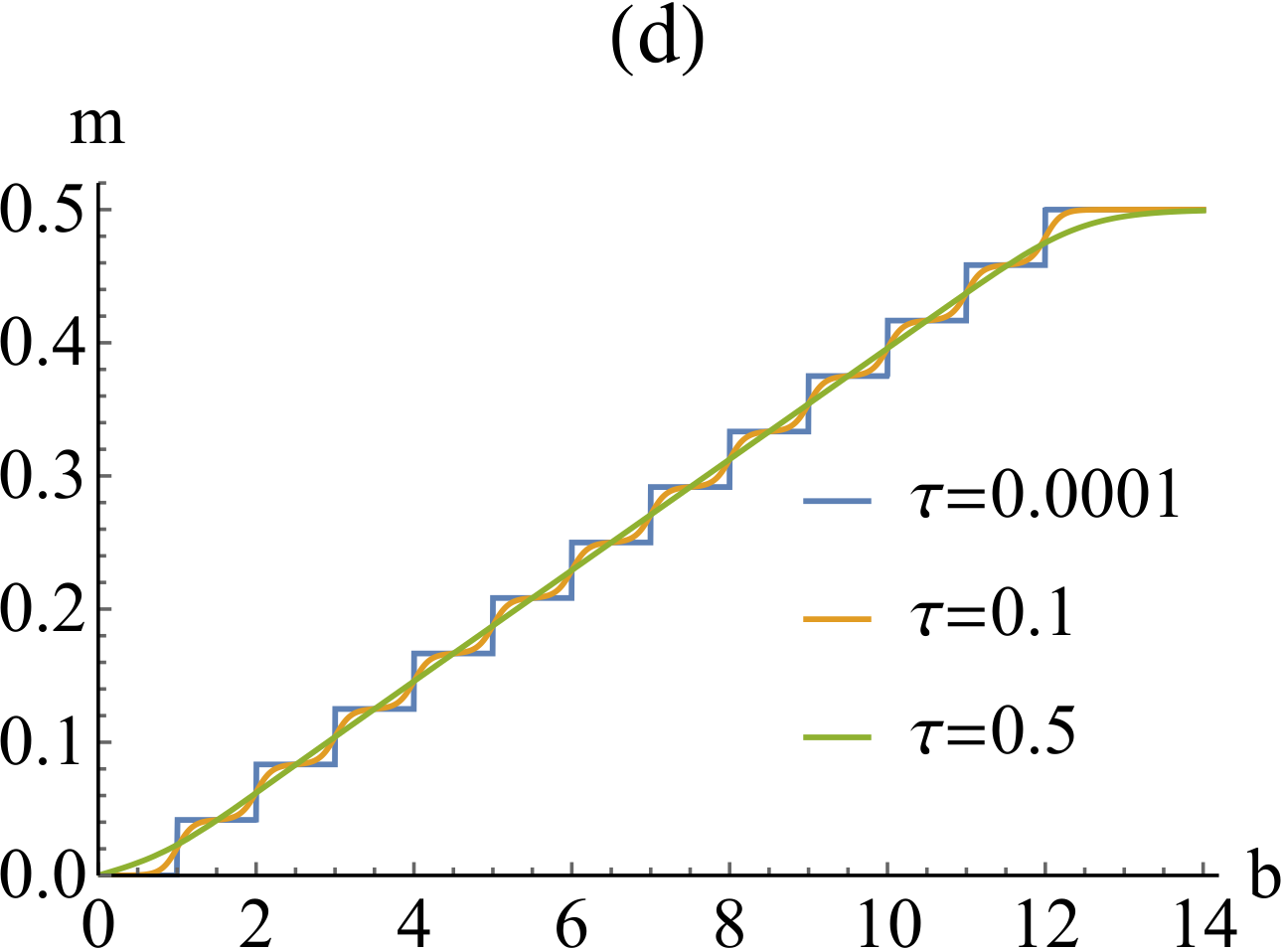
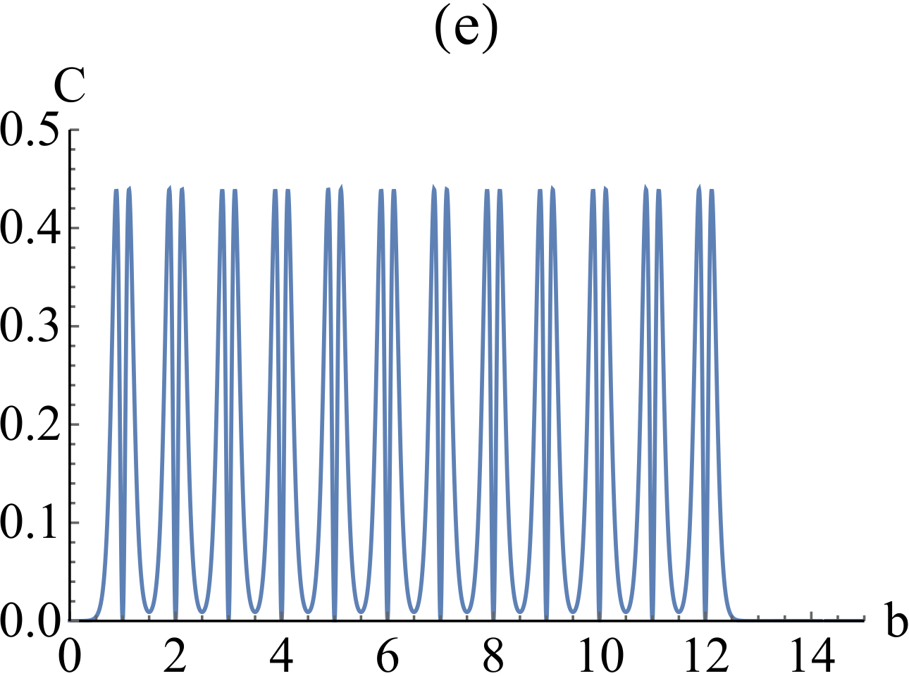
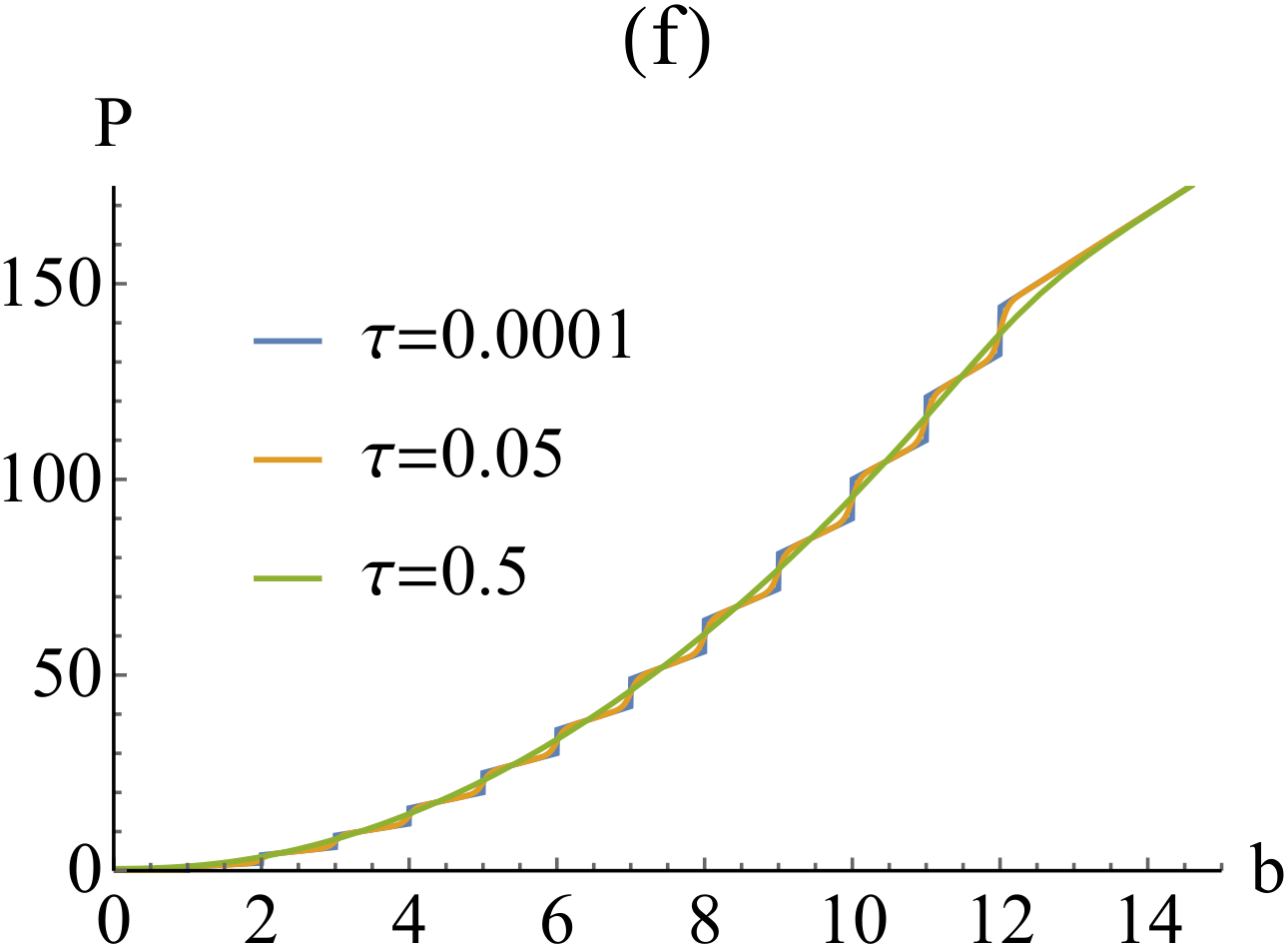
Figure 3: Thermodynamic quantities for $N=23,24$. (a)-(c) are for $N=23$ and $(d)-(f)$ are for $N=24$. The first column ((a),(d)) are the magnetization per particle $m$ vs. field $b$ for three temperatures $\tau=0.0001,0.1,0.5$. The second column ((b),(e)) shows the M shape in the specific heat $C$ vs. field $b$ for $\tau=0.05$. The third column ((c),(f)) shows the pressure $P$ vs. field $b$ for three temperatures $\tau=0.0001,0.05,0.5$.

Fig. 3 shows the full extension of the model to large particle number. Fig. 3(a) plots the magnetization per particle $m$ as a function of magnetic field at low temperatures for $N=23$. There is the expected step at $b=0$ followed by 11 more steps at $b=3/2,5/2,...,23/2$, which can be seen in both the magnetization per particle and the pressure in Fig. 3(c). The M shape in the specific heat (Fig. 3(b)) at small temperatures can be seen for each of the critical field values. The even $N$ case for the magnetization per particle, specific heat, and pressure using $N=24$ are seen in Figs. 3(d)-(f). Features similar to the $N=23$ case are seen for $N=24$.

The results here show that there will be steps at integer $b$ in the magnetization per particle and pressure which quickly blur with increased temperature. This implies an infinite number of steps in the thermodynamic limit. Since the change in the magnetization is the same in all cases, this means that the change in the magnetization per particle is always $1/N$, except for the initial $b=0$ change for odd $N$, which is $1/2N$. In the thermodynamic limit these steps are infinitesimally small for both even and odd $N$, implying that in the thermodynamic limit this model shows no metamagnetism.

V 5. Discussion and Conclusions

Metamagnetism in a strongly correlated metal derives its properties from the complicated interactions. It is usually described by a lattice of magnetic moments interacting with conduction electrons and often within a framework of Anderson model. The heavy mass of fermions is then an outcome of a Kondo-like effect. The ground state corresponds to a singlet resonance between the local moment and the conduction electrons. Metamagnetism happens when the magnetic field breaks the singlet resonance. This scenario is the basis of the microscopic calculations described Brenig:87 ; Ono:98 in several references. Several experimental correlations Aoki:13 ; Hirose:11 appear reasonable within this formalism. One outcome that remains to be explored experimentally is that between the critical field and the effective mass.

However in order to calculate a more complex observable, such as nonlinear susceptibilities, a truly microscopic calculation is a non-starter. An intermediate framework needs to be established which both transcends microscopic parameters and has the facility to proceed with more complex calculations. Described here is an orthogonal approach, studying a model that seems reasonable from a microscopic point of view but is simple enough to yield nonlinear susceptibilities.

The infinite range interaction model contains many of the properties one finds in metamagnetism. The model contains only one energy scale, $J$, apart from the thermodynamic control variables, the external magnetic field and the temperature. It is solvable with transparent intermediate steps. The notable features of this model are:

1. There is a quantum transition at $T=0$ that loses its singular transition properties at any non-zero temperature. Thus the $T=0$ transition is discontinuous in magnetization as well as in entropy. The total magnetic susceptibility $\chi(B,T=0)$ is singular at $B=B_{c}$. At any finite (non-zero) temperature, the magnetic susceptibility has maxima at $B=B_{c}$.

2. The nonlinear susceptibilities defined by

   $$M=\chi_{1}(T)B+\chi_{3}(T)B^{3}+\chi_{5}(T)B^{5}.$$

   are negative at high temperatures. They be come positive at low temperatures and go through a maximum.

3. There are features due to the oddness of the total number of particles $N$. For odd $N$, there is a free spin contribution to the susceptibility that diverges as $1/T$.

4. Finally there are results for the field dependence of the specific heat and pressure (from which the magnetic field dependence of the sound velocity can be derived).

The model is, in the classical sense, highly frustrated Chalker:11 . In the thermodynamic limit, there are no phase transitions as a function of temperature. This is due to the infinitesimal step size from an infinite number of transitions in $M$ in the thermodynamic limit. The model is a spin model that sidesteps the complexities of a real microscopic model for a strongly correlated fermion system. For a ferromagnetic version of this model ($J<0$) see Ref. . The objective here has been to develop a minimal (spins only) model which highlights the common features among materials with different lattice structures and electronic properties. The model may be useful in the fields of quantum magnetism Alcaraz:88 and molecular magnets Schnack:13 .

We acknowledge several stimulating and enlightening discussions with V. Celli, B. Cowan, B. Nartowt and B. Shivaram.

Appendix A Appendix A: Magnetization for odd $N$

The free spin term of the magnetization for odd particle number is able to be extracted (as in Eq. (7)) from $M(N=2n+1)$ in Eq. (6). The derivation of this is contingent upon three steps:

1. Rewrite the partition function $Z(N=2n+1)=\cosh(b/2\tau)F(b/\tau)$.

   The definition of $Z(N=2n+1)$ given in Eq. (5) is:

   $$Z(N=2n+1)=2\sum_{\mu=1/2}^{N/2}A_{\mu}(N)\cosh\left(\frac{\mu b}{\tau}\right).$$

   Since $A_{\mu}(N)$ is field independent, then the $\cosh(b/2\tau)$ must come from the $\cosh(\mu b/\tau)$ terms. Using the hyperbolic angle sum rules for $\cosh(x+y)$ and $\sinh(2x)$:

   $$\begin{split}\cosh(nb/\tau)&=\cosh((n-1)b/\tau)\cosh(b/\tau)+\sinh((n-1)b/\tau)\sinh(b/\tau),\\ &=\cosh((n-1)b/\tau)\cosh(b/\tau)+2\cosh(b/2\tau)\sinh((n-1)b/\tau)\sinh(b/2\tau).\end{split}$$

   Assuming that $\cosh((n-1)b/\tau)=\cosh(b/2\tau)f_{n-1}(b/\tau)$, then the above becomes:

   $$\begin{split}\cosh(nb/\tau)&=\cosh((n-1)b/\tau)\cosh(b/\tau)+2\cosh(b/2\tau)\sinh((n-1)b/\tau)\sinh(b/2\tau),\\ &=\cosh(b/2\tau)[f_{n-1}(b/\tau)\cosh(b/\tau)+2\sinh((n-1)b/\tau)\sinh(b/2\tau)].\end{split}$$

   The square brackets must then be $f_{n}(b/\tau)$, giving a recursion relation for $f_{n}(b/\tau)$:

   $$f_{n}(b/\tau)=f_{n-1}(b/\tau)\cosh(b/\tau)+2\sinh((n-1)b/\tau)\sinh(b/2\tau).$$ (14)

   By showing that this process is started using $n=1/2$ and $n=3/2$, the recursion can be proven true through induction. Using the relation $\cosh(nb/\tau)=\cosh(b/2\tau)f_{n}(b/\tau)$, the partition function can be rewritten:

   $$Z(N=2n+1)=\cosh(b/2\tau)\left[2\sum_{\mu=1/2}^{N/2}A_{\mu}(N)f_{\mu}(b/\tau)\right]=\cosh(b/2\tau)F(b/\tau).$$ (15)

2. Find a closed form for $F(b/\tau)$.

   The only unknown in $F(b/\tau)$ from Eq. (15) is the closed form of $f_{\mu}(b/\tau)$. This closed form is not obvious from Eq. (14). By rearranging the terms for $f_{3/2}(b/\tau)$ and $f_{5/2}(b/\tau)$, they can be rewritten using a nicer recursion relation:

   $$f_{n}(b/\tau)=2\cosh((n-1/2)b/\tau)-f_{n-1}(b/\tau),$$ (16)

   which has a straightforward closed form solution,

   $$f_{n}(b/\tau)=2\sum_{m=0}^{n-1/2}(-1)^{m}\cosh((n-1/2-m)b/\tau)-(-1)^{n-1/2}$$ (17)

   If this is the correct closed form for $f_{n}(b/\tau)$, then it will obey the original recursion of Eq. (14). Plugging Eq. (17) into the original recursion Eq. (14) and using the relation $\cosh(x)\cosh(y)=\cosh(x+y)-\sinh(x)\sinh(y)$ gives:

   $$\begin{split}f_{n}(b/\tau)&=\cosh(b/\tau)f_{n-1}(b/\tau)+2\sinh(b/2\tau)\sinh((n-1)b/\tau),\\ &=2\cosh((n-1/2)b/\tau)-\underbrace{2\sum_{m=1}^{n-3/2}(-1)^{m-1}\cosh((n-3/2-(m-1))b/\tau)}_{=f_{n-1}(b/\tau)-(-1)^{n-3/2}}+(-1)^{n-1/2}\cosh(b/\tau)\\ &\quad-2\sum_{m=0}^{n-3/2}(-1)^{m}\sinh((n-3/2-m)b/\tau)\sinh(b/\tau)+2\sinh(b/2\tau)\sinh((n-1)b/\tau),\\ &=2\cosh((n-1/2)b/\tau)-f_{n-1}(b/\tau)+S_{n},\end{split}$$

   where the extra term $S_{n}$ is

   $$S_{n}=(-1)^{n-3/2}+(-1)^{n-1/2}\cosh(b/\tau)-2\sum_{m=0}^{n-3/2}(-1)^{m}\sinh((n-3/2-m)b/\tau)\sinh(b/\tau)+2\sinh(b/2\tau)\sinh((n-1)b/\tau).$$

   This extra term is absent from Eq. (16), implying that $S_{n-1}=0$. It is straightforward to show that $S_{n}=0$ by considering $S_{n}=S_{n}+S_{n-1}$ and reducing. Since $S_{n}=0$, then Eq. (14) is the same recursion as Eq. (16), meaning that Eq. (17) is the closed form solution for $f_{n}(b/\tau)$.

3. Obtain the magnetization $M(N=2n+1)$

   Using Eq. (17) the partition function can be rewritten:

   $$\begin{split}Z(N=2n+1)&=\cosh(b/2\tau)\left[2\sum_{\mu=1/2}^{N/2}A_{\mu}(N)f_{\mu}(b/\tau)\right],\\ &=\cosh(b/2\tau)\left[B_{1/2}(N)+2\sum_{\mu^{\prime}=1}^{(N-1)/2}B_{\mu^{\prime}+1/2}(N)\cosh(\mu^{\prime}b/\tau)\right].\\ \end{split}$$ (18)

   The coefficients $B_{n}(N)$ are related to the coefficients $A_{n}(N)$:

   $$B_{n}(N)=2\sum_{m=n}^{N/2}(-1)^{m}A_{m}(N)\quad\longleftrightarrow\quad A_{n}(N)=\frac{1}{2}(B_{n}(N)+B_{n+1}(N)).$$

   This leaves the derivation of the magnetization $M(N=2n+1)$. This can be done by taking the derivative of the natural log of the new form for the partition function from above. Taking this derivative:

   $$\frac{M(N=2n+1)}{\gamma}=\tau\frac{\partial}{\partial b}\ln(Z(N))=\frac{1}{2}\tanh(b/2\tau)+\frac{2\sum_{\mu=1}^{(N-1)/2}\mu B_{\mu+1/2}(N)\sinh(\mu b/\tau)}{B_{1/2}(N)+2\sum_{\mu=1}^{(N-1)/2}B_{\mu+1/2}(N)\cosh(\mu b/\tau)}.$$ (19)

   which is exactly the form provided in Eq. (7). The second term resembles $M(N=2n)$ in Eq. (6) if $A_{\mu}(N=2n)$ is replaced with $B_{\mu+1/2}(N=2n+1)$.

Appendix B Appendix B: Steps in the magnetization

For all cases presented, steps in the magnetization occur at integer values of the dimensionless field $b=\gamma B/J$ for even particle number and half-integer values of $b$ for odd particle number. A change in the ground state energy creates a change in the magnetization. This is because the ground state energy provides the largest weight to the partition function in the low temperature limit $T\rightarrow 0$. The critical field values can be determined by when there is change in the ground state energy.

For an even number of particles, the eigenenergies are:

$$\lambda=\frac{J}{2}S(S+1)-\gamma\mu B,\quad\quad 0\leq S\leq N/2,\text{ }-S\leq\mu\leq S,$$

where $S$ is the total spin of the system and $\mu$ is the $z$-component of the total spin. The constant term $3JN/8$ does not affect this proof and thus was dropped. For any given value of $S$, the smallest eigenenergy takes $\mu=S$. For $B=0$ the smallest eigenenergy is simply $\lambda=0$. A new ground state occurs when a higher energy level crosses this energy level. The crossover locations for $S>0$ with the $S=0$ level are:

$$0=\frac{J}{2}S(S+1)-\gamma SB\quad\rightarrow\quad B=\frac{J}{2\gamma}(S+1),$$

The first crossing will create a new ground state energy level, occurring for $S=1$, or $B_{c}=\frac{J}{\gamma}$. Another new ground state will occur when a higher energy level ($S>1$) crosses the $S=1$ ground state energy level. All crossings can be calculated:

$$\begin{split}&\frac{J}{2}(1)(2)-\gamma(1)B=\frac{J}{2}S(S+1)-\gamma SB.\\ \rightarrow&B=\frac{J}{2\gamma}\frac{S(S+1)-2}{S-1}=\frac{J}{2\gamma}(S+2).\end{split}$$

The next highest spin ($S=2$) will create the next ground state energy at the crossing $B_{c}=2J/\gamma$. When a ground state takes spin $S_{g}$ the next ground state will have $S>S_{g}$ through induction:

$$\begin{split}&\frac{J}{2}(S_{g})(S_{g}+1)-\gamma(S_{g})B=\frac{J}{2}S(S+1)-\gamma SB,\\ \rightarrow&B=\frac{J}{2\gamma}\left(S+S_{g}+1\right).\end{split}$$

The next ground state will then always be for $S=S_{g}+1$ at the crossing $B_{c}=(S_{g}+1)J/\gamma=nJ/\gamma$. Although this proof is for an even particle number $N$, an equivalent proof can be performed for odd $N$ to show the half integer crossings. The value of the magnetization for $T\rightarrow 0$ will be equal to the value of $S_{g}$ since $M=\frac{1}{\beta}\partial_{B}\ln Z$ for small $T$ is approximated by the ground state:

$$\begin{split}M(B,T\rightarrow 0)&\approx\frac{1}{\beta}\frac{\partial_{B}e^{-\beta JS_{g}(S_{g}+1)/2+\gamma\beta BS_{g}}}{e^{-\beta JS_{g}(S_{g}+1)/2+\gamma\beta BS_{g}}},\\ &\approx\gamma S_{g}\frac{e^{-\beta JS_{g}(S_{g}+1)/2+\gamma\beta BS_{g}}}{e^{-\beta JS_{g}(S_{g}+1)/2+\gamma\beta BS_{g}}},\\ &\approx\gamma S_{g}.\end{split}$$

References

- (1) E. Stryjewski and N. Giordano, Advances in Physics 26, 487 (1977).
- (2) R. Z. Levitin and A. S. Markosyan, Soviet Physics Uspekhi 31, 730 (1988).
- (3) T. Goto, K. Fukamichi, and H. Yamada, Physica B: Condensed Matter 300, 167 (2001), jubilee issue Volume 300.
- (4) E. P. Wohlfarth and P. Rhodes, Philosophical Magazine 7, 1817 (1962).
- (5) D. Aoki, W. Knafo, and I. Sheikin, Comptes Rendus Physique 14, 53 (2013), physics in High Magnetic Fields / Physique en champ magnétique intense.
- (6) A. W. Rost et al., Science 325, 1360 (2009).
- (7) S. M. Thomas et al., Phys. Rev. B 93, 075149 (2016).
- (8) A. J. Millis, A. J. Schofield, G. G. Lonzarich, and S. A. Grigera, Phys. Rev. Lett. 88, 217204 (2002).
- (9) E. D’Hoker and P. Kraus, Journal of High Energy Physics 2010, 83 (2010).
- (10) P. Bak and R. Bruinsma, Phys. Rev. Lett. 49, 249 (1982).
- (11) B. S. Shivaram, B. Dorsey, D. G. Hinks, and P. Kumar, Phys. Rev. B 89, 161108 (2014).
- (12) Y. Hirose et al., Journal of Physics: Conference Series 273, 012003 (2011).
- (13) A. Thamizhavel et al., arxiv:1510.02991 (2015).
- (14) B. Shivaram, arxiv:1510.04755 (2015).
- (15) J. Schnack, in Emergent Phenomena in Correlated Matter, edited by E. Pavarini, E. Koch, and U. Schollwock (Forschungszentrum Julich, Julich, Germany, 2013), pp. 8.1–8.39.
- (16) F. C. Alcaraz, M. N. Barber, and M. T. Batchelor, Annals of Physics 182, 280 (1988).
- (17) B. Bleaney and K. D. Bowers, Proceedings of the Royal Society of London A: Mathematical, Physical and Engineering Sciences 214, 451 (1952).
- (18) M. Tachiki and T. Yamada, Journal of the Physical Society of Japan 28, 1413 (1970).
- (19) W. Brenig, Solid State Communications 64, 203 (1987).
- (20) Y. Ono, Journal of the Physical Society of Japan 67, 2197 (1998).
- (21) J. T. Chalker, in Introduction to Frustrated Magnetism: Materials, Experiments, Theory, edited by C. Lacroix, P. Mendels, and F. Mila (Springer Berlin Heidelberg, Berlin, Heidelberg, 2011), pp. 3–22.