Full likelihood inference for max-stable data

Raphaël Huser¹, Clément Dombry², Mathieu Ribatet³, Marc G. Genton¹

March 18, 2024

We show how to perform full likelihood inference for max-stable multivariate distributions or processes based on a stochastic Expectation-Maximisation algorithm, which combines statistical and computational efficiency in high-dimensions. The good performance of this methodology is demonstrated by simulation based on the popular logistic and Brown–Resnick models, and it is shown to provide dramatic computational time improvements with respect to a direct computation of the likelihood. Strategies to further reduce the computational burden are also discussed.

Keywords: Full likelihood; Max-stable distribution; Stephenson–Tawn likelihood; Stochastic Expectation-Maximisation algorithm.

1 Introduction

Under mild conditions, max-stable distributions and processes are useful for studying high-dimensional extreme events recorded in space and time (Padoan et al., 2010; Davis et al., 2013; Davison et al., 2013; de Carvalho and Davison, 2014; Huser and Davison, 2014; Huser and Genton, 2016). This broad but constrained class of models may, at least theoretically, be used to extrapolate into the joint tail, hence providing a justified framework for risk assessment of extreme events. The probabilistic justification is that the max-stable property arises in limiting models for suitably renormalised maxima of independent and identically distributed processes; see, e.g., Davison et al. (2012), Davison and Huser (2015) and Davison et al. (2018).

Because extremes are rare by definition, it is crucial for reliable estimation and prediction to extract as much information from the data as possible. Thus, efficient estimators play a particularly important role in statistics of extremes, and the maximum likelihood estimator is a natural choice thanks to its appealing large-sample properties. However, the likelihood function is excessively difficult to compute for high-dimensional data following a max-stable distribution. As detailed in §3, likelihood evaluations require the computation of a sum indexed by all elements of a given set ${\mathcal{P}}_{D}$, the cardinality of which grows more than exponentially with the dimension, $D$. In a thorough simulation study, Castruccio et al. (2016) stated that current technologies are limiting full likelihood inference to dimension $12$ or $13$, and they concluded that without meaningful methodological advances, a direct full likelihood approach will not be feasible.

To circumvent this computational bottleneck, several strategies have been advocated. Padoan et al. (2010) proposed a pairwise likelihood approach, combining the bivariate densities of carefully chosen pairs of observations. Although this method is computationally attractive and inherits many good properties from the maximum likelihood estimator, it also entails a loss in efficiency, which becomes more apparent in high dimensions (Huser et al., 2016). More efficient triplewise and higher-order composite likelihoods were investigated by Genton et al. (2011), Huser and Davison (2013), Sang and Genton (2014) and Castruccio et al. (2016). However, they are still not fully efficient, and it is not clear how to optimally select the composite likelihood terms. Furthermore, because composite likelihoods are generally not valid likelihoods (Varin et al., 2011), the classical likelihood theory cannot be blindly applied for uncertainty assessment, testing, model validation and selection, and so forth.

Alternatively, Stephenson and Tawn (2005) suggested augmenting the componentwise block maxima data $z^{n}=(z_{1}^{n},\ldots,z_{D}^{n})^{\rm T}$, where $n$ is the block size, with their occurrence times. This extra information may be summarized by an observed partition $\pi^{n}$ of the set $\{1,\ldots,D\}$, which indicates whether or not these maxima occurred simultaneously. Essentially, the Stephenson–Tawn likelihood corresponds the limiting joint “density” of $z^{n}$ and $\pi^{n}$, as $n\to\infty$, and it yields drastic simplifications and improved efficiency. However, Wadsworth (2015) and Huser et al. (2016) noted that this approach may be severely biased for finite $n$, especially in low-dependence scenarios. By fixing the limit partition, $\pi$, to the observed one, $\pi^{n}$, a strong constraint is imposed, creating model misspecification, to which likelihood methods are sensitive.

In this paper, to mitigate the sub-asymptotic bias due to fixing the partition, we suggest returning to the original likelihood formulation, which integrates out the partition rather than treating it as known. By interpreting the limit partition $\pi$ as missing data, we show how to design a stochastic Expectation-Maximisation algorithm (Dempster et al., 1977; Nielsen, 2000) for efficient inference. The quality of the stochastic approximation to the full likelihood can be controlled and set to any arbitrary precision at a computational cost. We show that higher-dimensional max-stable models may be fitted in reasonable time. Importantly, our method is based solely on max-stable data and does not require extra information about the partition or the original processes, unlike the Stephenson–Tawn or related threshold-based methods. Our approach is based on the algorithm of Dombry et al. (2013) for conditional simulation of the partition given the data, and it is closely related to the recent papers of Thibaud et al. (2016) and Dombry et al. (2017a), who in a Bayesian setting developed a Markov chain Monte Carlo algorithm for max-stable processes by treating the partition as a latent variable to be resampled at each iteration.

2 Max-stable processes and distributions

2.1 Definition, construction, and models

Consider a sequence of independent and identically distributed processes $Y_{1}(s),Y_{2}(s),\ldots,$ indexed by spatial site $s\in{\mathcal{S}}\subset{}^{d}$, and assume that there exist sequences of functions $a_{n}(s)>0$ and $b_{n}(s)$, such that the renormalised pointwise block maximum process (with block size $n$)

$$Z^{n}(s)=a_{n}(s)^{-1}\left[\max\{Y_{1}(s),\ldots,Y_{n}(s)\}-b_{n}(s)\right]$$ (1)

converges in the sense of finite-distributional distributions, as $n\to\infty$, to a process $Z(s)$ with non-degenerate marginal distributions, i.e., $Y(s)$ is in the max-domain of attraction of $Z(s)$. Then, the limit $Z(s)$ is max-stable (see, e.g., de Haan and Ferreira, 2006, Chap. 9). That is, pointwise maxima of independent copies of the limit process $Z(s)$ have the same dependence structure as $Z(s)$ itself, while marginal distributions are in the same location-scale family and coincide with the generalized extreme-value distribution.

Consider now points of a unit rate Poisson point process, $P_{1},P_{2},\ldots$, and independent copies, $W_{1}(s),W_{2}(s),\ldots$, of a stochastic process $W(s)\geq 0$ with unit mean. Then, the process

$$Z(s)=\sup_{j\geq 1}W_{j}(s)/P_{j},\quad s\in{\mathcal{S}},$$ (2)

is max-stable with unit Fréchet marginal distributions, i.e., ${\rm Pr}\{Z(s)\leq z\}=\exp(-1/z)$, $z>0$ (de Haan, 1984; Schlather, 2002). In the remaining of the paper, we shall always consider max-stable processes $Z(s)$ with unit Fréchet marginal distributions. Representation (2) is useful to build a wide variety of max-stable processes (Smith, 1990; Schlather, 2002; Kabluchko et al., 2009; Opitz, 2013; Xu and Genton, 2016), and to simulate from them (Schlather, 2002; Dombry et al., 2016). Multivariate max-stable models can be constructed similarly. From (2), we deduce that the joint distribution at a finite set of sites ${\mathcal{S}}_{D}=\{s_{1},\ldots,s_{D}\}\subset{\mathcal{S}}$ may be expressed as

$${\rm Pr}\{Z(s_{1})\leq z_{1},\ldots,Z(s_{D})\leq z_{D}\}=\exp\{-V(z_{1},\ldots,z_{D})\},$$ (3)

where the exponent function $V(z_{1},\ldots,z_{D})=E\left[\max\left\{{W(s_{1})/z_{1}},\ldots,{W(s_{D})/z_{D}}\right\}\right]$ satisfies homogeneity and marginal constraints (see, e.g., Davison and Huser, 2015). As an illustration, Fig. 1 shows two independent realisations from the same Smith (1990) model defined by taking $W_{j}(s)=\phi(s-U_{j};\sigma^{2})$, $s\in{\mathcal{S}}=\Real$, in (2), where $\phi(\cdot;\sigma^{2})$ is the normal density with zero mean and variance $\sigma^{2}$, and the $U_{j}$s are points from a unit rate Poisson point process on the real line.

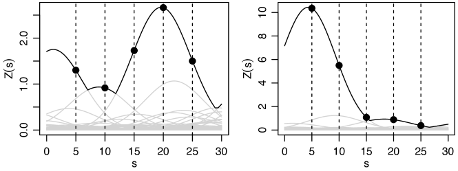
Figure 1: Two realisations (black) from the same Smith (1990) max-stable process on the line defined by setting $W(s)=\phi(s-U;\sigma^{2})$, $s\in{\mathcal{S}}=\Real$, in (2), with the latent profiles $W_{j}(s)/P_{j}$ (grey). Here, $\sigma^{2}=5$. When observed at sites $5,10,15,20,25$, the partitions are $\pi=\{\{1\},\{2\},\{3,4,5\}\}$ (left) and $\pi=\{\{1,2,3\},\{4,5\}\}$ (right).

2.2 Underlying partition and extremal functions

At each site $s\in{\mathcal{S}}$, the pointwise supremum, $Z(s)$, in (2) is realised by a single profile $W_{j}(s)/P_{j}$ almost surely. Such profiles are called extremal functions in Dombry et al. (2013). As illustrated in Fig. 1, the extremal functions are only partially observed on ${\mathcal{S}}_{D}=\{s_{1},\ldots,s_{D}\}$; they define a random partition $\pi=\{\tau_{1},\ldots,\tau_{|\pi|}\}$ (of size $|\pi|$) of the set $\{1,\ldots,D\}$, called hitting scenario in Dombry et al. (2013) that identifies clusters of variables stemming from the same event. For example, the partition $\pi=\{\{1\},\{2\},\{3,4,5\}\}$ on the left panel of Fig. 1 indicates that the max-stable process at these five sites came from three separate independent events; in particular, the maxima at $s_{3}=15$, $s_{4}=20$, and $s_{5}=25$ were generated from the same profile.

Similarly, an observed partition $\pi^{n}$ of $\{1,\ldots,D\}$ may be defined for $Z^{n}(s)$ in (1) based on the original processes $Y_{1}(s),\ldots,Y_{n}(s)$. The knowledge of $\pi^{n}$ tells us if extreme events at different sites occurred simultaneously or not, so $\pi^{n}$ carries information about the strength of spatial extremal dependence. If the processes $Y_{1}(s),\ldots,Y_{n}(s)$ (suitably marginally transformed) are in the max-domain of attraction of $Z(s)$ in (2), then the partition $\pi^{n}$ converges in distribution to $\pi$, as $n\to\infty$, on the space of all partitions ${\mathcal{P}}_{D}$ of $\{1,\ldots,D\}$ (Stephenson and Tawn, 2005).

We now describe likelihood inference for max-stable vectors: by exploiting the information on the partition $\pi$ (Stephenson–Tawn likelihood), or by integrating it out (full likelihood).

3 Likelihood inference

3.1 Full and Stephenson–Tawn likelihoods

By differentiating the distribution (3) with respect to the variables $z_{1},\ldots,z_{D}$, we can deduce that the corresponding density, or full likelihood for one replicate, may be expressed as

$$g_{\rm Full}(z_{1},\ldots,z_{D})=\exp\{-V(z_{1},\ldots,z_{D})\}\sum_{\pi\in{\mathcal{P}}_{D}}\prod_{i=1}^{|\pi|}\{-V_{\tau_{i}}(z_{1},\ldots,z_{D})\},$$ (4)

where $V_{\tau_{i}}$ denotes the partial derivative of the function $V$ with respect to the variables indexed by the set $\tau_{i}\subset\{1,\ldots,D\}$ (Huser et al., 2016; Castruccio et al., 2016). The sum in (4) is taken over all elements of ${\mathcal{P}}_{D}$, the size of which equals the Bell number of order $D$, leading to an explosion of terms, even for moderate $D$. Each term in (4) corresponds to a different configuration of the profiles $W_{j}(s)/P_{j}$ in (2) at the sites $s_{1},\ldots,s_{D}$. Thus, Castruccio et al. (2016) argued that the computation of (4) is limited to dimension $12$ or $13$ with modern computational resources.

As detailed in the Supplementary Material using a point process argument, and originally shown by Stephenson and Tawn (2005), the joint density of the max-stable data $z=(z_{1},\ldots,z_{D})^{\rm T}$ and the associated partition $\pi=\{\tau_{1},\ldots,\tau_{|\pi|}\}\in{\mathcal{P}}_{D}$ is simply equal to

$$g_{\rm ST}(z_{1},\ldots,z_{D},\pi)=\exp\{-V(z_{1},\ldots,z_{D})\}\prod_{i=1}^{|\pi|}\{-V_{\tau_{i}}(z_{1},\ldots,z_{D})\},$$ (5)

hence reducing the problematic sum to a single term, making likelihood inference possible in higher dimensions and simultaneously improving statistical efficiency. Because the asymptotic partition $\pi$ is not observed, Stephenson and Tawn (2005) suggested replacing it by the observed partition $\pi^{n}$ of occurrence times of maxima, which converges to $\pi$ provided the asymptotic model is well specified. However, Wadsworth (2015) and Huser et al. (2016) showed that lack of convergence of $\pi^{n}$ to $\pi$ may result in severe estimation bias, which is especially strong in low-dependence cases. To circumvent this problem, Wadsworth (2015) proposed a bias-corrected likelihood; alternatively, we show in the next section how to design a stochastic Expectation-Maximisation algorithm to maximise (4), while taking advantage of the computationally appealing nature of (5).

3.2 Stochastic Expectation-Maximisation algorithm

It is instructive to rewrite the full likelihood (4) using (5) as $g_{\rm Full}(z_{1},\ldots,z_{D})=\sum_{\pi\in{\mathcal{P}}_{D}}g_{\rm ST}(z_{1},\ldots,z_{D},\pi)$ because it highlights that the full likelihood simply integrates out the latent random partition $\pi$ needed for the Stephenson–Tawn likelihood. Interpreting $\pi$ as a missing observation and the Stephenson–Tawn likelihood as the completed likelihood, an Expectation-Maximisation algorithm (Dempster et al., 1977) may be easily formulated. Assume that the exponent function $V(z_{1},\ldots,z_{D}\mid\theta)$ is parametrised by a vector $\theta\in\Theta\subset{}^{p}$. Starting from an initial guess $\theta_{0}\in\Theta$, the Expectation-Maximisation algorithm consists of iterating the following E- and M-steps for $r=1,\ldots,R$:

• E-step: compute the functional

  $$Q(\theta,\theta_{r-1})=E_{\pi\mid z,\theta_{r-1}}\left[\log\left\{g_{\rm ST}(z,\pi\mid\theta)\right\}\right]=\sum_{\pi\in{\mathcal{P}}_{D}}g(\pi\mid z,\theta_{r-1})\log\{g_{\rm ST}(z,\pi\mid\theta)\},$$ (6)

  where the expectation is computed with respect to the discrete conditional distribution of $\pi$ given the data $z=(z_{1},\ldots,z_{D})^{\rm T}$ and the current value of the parameter $\theta_{r-1}$, i.e.,

  $$g(\pi\mid z,\theta_{r-1})={g_{\rm ST}(z,\pi\mid\theta_{r-1})/g_{\rm Full}(z\mid\theta_{r-1})}.$$ (7)

• M-step: update the parameter as $\theta_{r}=\arg\max_{\theta\in\Theta}Q(\theta,\theta_{r-1})$.

Dempster et al. (1977) showed that the Expectation-Maximisation algorithm has appealing properties; in particular, the value of the log-likelihood increases at each iteration, which ensures convergence of $\theta_{r}$ to a local maximum, as $r\to\infty$. In our case, however, the expectation in (6) is tricky to compute: it contains again the sum over the set ${\mathcal{P}}_{D}$, and (7) relies on the full density $g_{\rm Full}(z\mid\theta_{r-1})$, which we try to avoid. To circumvent this issue, one solution is to approximate (6) by Monte Carlo as

$${\widehat{Q}}(\theta,\theta_{r-1})={1\over N}\sum_{i=1}^{N}\log\left\{g_{\rm ST}(z,\pi_{i}\mid\theta)\right\},\quad\pi_{1},\ldots,\pi_{N}\sim g(\pi\mid z,\theta_{r-1}),$$ (8)

where the partitions $\pi_{1},\ldots,\pi_{N}$ are conditionally independent at best, or form an ergodic sequence at least. As $g(\pi\mid z,\theta_{r-1})\propto g_{\rm ST}(z,\pi\mid\theta_{r-1})$, see (7), it is possible to devise a Gibbs sampler to generate approximate simulations from $g(\pi\mid z,\theta_{r-1})$ without explicitly computing the constant factor $g_{\rm Full}(z\mid\theta_{r-1})$ in the denominator of (7). Thanks to ergodicity of the resulting Markov chain, the precision of the approximation (8) may be set arbitrarily high by letting $N\to\infty$ (and discarding some burn-in iterations). More details about the practical implementation of the Gibbs sampler are given in Dombry et al. (2013) and in the Supplementary Material. Although the number of iterations of the Gibbs sampler, $N$, will typically be much smaller than the cardinality of ${\mathcal{P}}_{D}$, the approximation (8) to (6) will likely be reasonably good for moderate values of $N$ because only a few partitions $\pi\in{\mathcal{P}}_{D}$ may be plausible or compatible with the data $z=(z_{1},\ldots,z_{D})^{\rm T}$.

The asymptotic properties of the stochastic Expectation-Maximisation estimator, ${\widehat{\theta}}_{\rm SEM}$, were studied in details by Nielsen (2000) and compared with the classical maximum likelihood estimator, ${\widehat{\theta}}$; see §2–3 therein, in particular Theorem 2. Dombry et al. (2017b) showed that the maximum likelihood estimator ${\widehat{\theta}}$ is consistent and asymptotically normal for the most popular max-stable models, including the logistic and Brown–Resnick models used in this paper. This suggests that these appealing asymptotic properties should also be satisfied for the estimator ${\widehat{\theta}}_{\rm SEM}$, provided some additional rather technical regularity conditions detailed in Nielsen (2000) are satisfied. If so, then the asymptotic performance of ${\widehat{\theta}}_{\rm SEM}$ is akin to that of ${\widehat{\theta}}$, though with a larger asymptotic variance. Finally, the inherent variability of the stochastic Expectation-Maximisation algorithm may also be a blessing: unlike the deterministic Expectation-Maximisation algorithm, it is less likely to get stuck at a local maximum of the full likelihood.

4 Simulation study

To assess the performance of the stochastic Expectation-Maximisation estimator ${\widehat{\theta}}_{\rm SEM}$, we simulated data from the multivariate logistic max-stable distribution with exponent function $V(z_{1},\ldots,z_{D}\mid\theta)=(\sum_{j=1}^{D}z_{j}^{-1/\theta})^{\theta}$, $\theta\in\Theta=(0,1]$. Here, the parameter $\theta$ controls the dependence strength, with $\theta\to 0$ and $\theta=1$ corresponding to perfect dependence and independence, respectively. This model was chosen for two main reasons: first, it is the simplest max-stable distribution, often used as a benchmark, that interpolates between perfect dependence and independence; and second, the full likelihood (4) can be efficiently computed in this case using a recursive algorithm (Shi, 1995), thus allowing us to compare ${\widehat{\theta}}_{\rm SEM}$ and ${\widehat{\theta}}$ in high dimensions. Further results for the popular and more realistic, but computationally demanding, spatial max-stable model known as Brown–Resnick model (Kabluchko et al., 2009), are reported in the Supplementary Material. All simulations presented below and in the Supplementary Material were performed in parallel on the KAUST Cray XC40 supercomputer Shaheen II.

We first investigated the performance of the estimator ${\widehat{\theta}}_{\rm SEM}$ under different scenarios. We considered dimensions $D=2,5,10,20$, with $20$ independent temporal replicates, and $\theta=0.1,\ldots,0.9$ (strong to weak dependence). Setting the initial value to $\theta_{0}=0.6$, we chose $R=30$ iterations for the Expectation-Maximisation algorithm, averaging the last $5$ iterations, and took $110\times D$ iterations for the underlying Gibbs sampler. Following simulations reported in the Supplementary Material, we discarded the first $10\times D$ iterations as burn-in, and thinned the Markov chain by a factor $D$, in order to keep $N=100$ roughly independent partitions $\pi_{i}$ to compute (8). We repeated the experiment $1024$ times to estimate the bias, ${\rm B}$, standard deviation, ${\rm SD}$, root mean squared error, ${\rm RMSE}=({\rm B}^{2}+{\rm SD}^{2})^{1/2}$, and relative error with respect to the maximum likelihood estimator, ${\rm RE}=E|({\widehat{\theta}}_{\rm SEM}-{\widehat{\theta}})/{\widehat{\theta}}|$. Figure 2 reports the results. As expected, the bias is negligible compared to the standard deviation, and the latter decreases with increasing dimension $D$ but increases as the data approach independence ($\theta\to 1$). The RMSE (not shown) is almost only determined by the standard deviation. The relative error is always very small (uniformly less than about $0.6\%$), and it decreases for the most part with $D$ and also with $N$ as suggested by further unreported simulations.

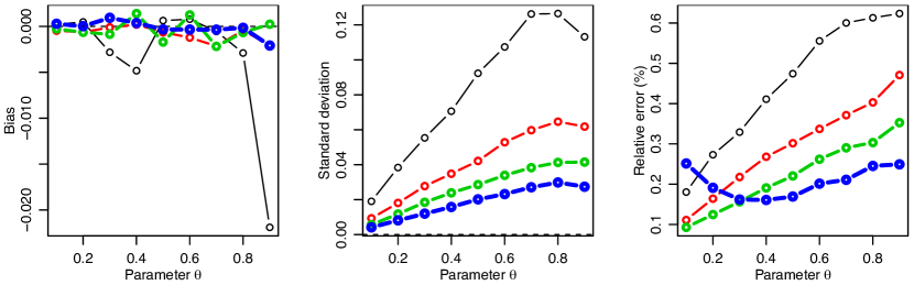
Figure 2: Performance of the estimator ${\widehat{\theta}}_{\rm SEM}$: bias (left), standard deviation (middle) and relative error in $\%$ (right), for the logistic model with $\theta=0.1,\ldots,0.9$ in dimension $D=2$ (thinnest black), $5$ (thin red), $10$ (thick green) and $20$ (thickest blue), based on $20$ independent temporal replicates. The number of iterations for the Expectation-Maximisation algorithm was set to $R=30$, averaging the last $5$ iterations, and the number of iterations of the underlying Gibbs sampler was set to $110\times D$ (thinned by a factor $D$, after a burn-in of $10\times D$). The initial value was set to $\theta_{0}=0.6$.

We now turn our attention to the computational efficiency of the stochastic Expectation-Maximisation algorithm. Considering dimensions up to $D=100$ under the exact same setting as before, the leftmost panel of Fig. 3 shows that it takes on average $5$–$6$ minutes to compute ${\widehat{\theta}}_{\rm SEM}$ (on a single core with 2.3GHz) when $D=100$ and $\theta=0.9$. Recall that, according to Castruccio et al. (2016), a direct evaluation of the likelihood (4) is not possible in dimensions greater than $D=12$ or $13$, thus this result is a big improvement over the current existing methods. The computational time appears to be roughly linear with $D$, which is due to the number of iterations of the Gibbs sampler set proportional to $D$. However, for more complex models such as the Brown–Resnick model, the computational time is significantly larger; see the Supplementary Material. Therefore, it makes sense to seek strategies to reduce the computational burden. One possibility is to tune the number of iterations of the stochastic Expectation-Maximisation algorithm. To investigate its speed of convergence, the two middle panels of Fig. 3 show the sample path $r\mapsto\theta_{r}$ for the logistic model as a function of the iteration $r=1,\ldots,50$, centred by the average over iterations $30$–$50$ for $100$ independent runs in dimension $D=10$. The true values were set to $\theta=0.3$ (second panel) and $0.9$ (third panel), and the initial value was set to $\theta_{0}=0.6$. The convergence is quite fast when $\theta=0.3$, requiring about $5$ iterations, but when $\theta=0.9$, it takes between $15$ and $25$ iterations. Simulations reported in the Supplementary Material suggest that although the Brown–Resnick has $p=2$ parameters, the number of iterations needed for the algorithm to converge is roughly the same. Another possibility to reduce the computational time is to play with the number of iterations of the underlying Gibbs sampler, which is the main computational bottleneck of this approach. The rightmost panel of Fig. 3 displays estimated parameters in dimension $D=10$ with associated $95\%$ confidence intervals for $\theta=0.3,0.6,0.9$, using $30$ Expectation-Maximisation iterations and $(N+10)\times D$ iterations for the underlying Gibbs sampler with $N=2,5,10,20,50,100,200,500,1000$. Again, we discarded the first $10\times D$ iterations as burn-in and we thinned the resulting chain by a factor $D$. Surprisingly, the distribution of ${\widehat{\theta}}_{\rm SEM}$ is almost stable for all $N\geq 2$, suggesting that the number of Gibbs iterations does not need to be very large for accurate estimation. Overall, significant computational savings can be achieved without any loss of accuracy, by suitably choosing $R$ (Expectation-Maximisation iterations) and $N$ (Gibbs iterations).

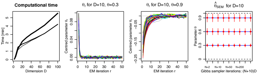
Figure 3: Left: Computational time for computing ${\widehat{\theta}}_{\rm SEM}$ for the logistic model, as function of dimension $D$, for $\theta=0.3$ (thin), $0.6$ (medium), $0.9$ (thick). We used $20$ temporal replicates, $30$ Expectation-Maximisation iterations, and $110\times D$ iterations for the underlying Gibbs sampler. Middle panels: parameter values $\theta_{r}$ as function of iteration $r=1,\ldots,50$, centred by the average over iterations $30$–$50$, for $100$ independent runs in dimension $D=10$. True values were set to $\theta=0.3$ (second panel) and $0.9$ (third panel), and the initial value was set to $\theta_{0}=0.6$. Right: Mean of estimated parameters ${\widehat{\theta}}_{\rm SEM}$ (red dots) with $95\%$ confidence intervals for $\theta=0.3,0.6,0.9$, dimension $D=10$, $30$ Expectation-Maximisation iterations, and $(N+10)\times D$ Gibbs sampler iterations with $N=2,5,10,20,50,100,200,500,1000$ (x-axis). In all simulations, we always thinned the underlying Markov chains by a factor $D$ after discarding a burn-in of $10\times D$ iterations.

5 Discussion

To resolve the problem of inference for max-stable distributions and processes, we have proposed a stochastic Expectation-Maximisation algorithm, which does not fix the underlying partition, but instead, treats it as a missing observation, and integrates it out. The beauty of this approach is that it combines statistical and computational efficiency in high dimensions, and it does not suffer from misspecification entailed by lack of convergence of the partition. As a proof of concept, we have validated the methodology by simulation based on the logistic model, and we have shown that in this case it is easy to make inference beyond dimension $D=100$ in just a few minutes. In the Supplementary Material, we have also provided results for the popular Brown–Resnick spatial max-stable model. In this case, our full likelihood inference approach can handle dimensions up to about $D=20$ in a reasonable amount of time. The difficulty resides in the computation of high-dimensional multivariate Gaussian distributions needed for $V$ and $V_{\tau_{i}}$. Unbiased Monte Carlo estimates of these quantities can be obtained, and Thibaud et al. (2016) and de Fondeville and Davison (2018) suggest using crude approximations to reduce the computational time while maintaining accuracy; see also Genton et al. (2018). Our method is not limited to these two models and could potentially be applied to any max-stable model for which the exponent function $V$ and its partial derivatives $V_{\tau_{i}}$ are available. The main computational bottleneck of our approach is that we need to generate a Gibbs sampler for each independent temporal replicate of the process. Fortunately, as this setting is embarrassingly parallel, we may thus easily take advantage of available distributed computing resources. Finally, there is a large volume of literature on the stochastic Expectation-Maximisation algorithm, and it might be possible to devise automatic stopping criteria and adaptive schemes for the Gibbs sampler to further speed up the algorithm (Booth and Hobert, 1999).

Supplementary material

Supplementary Material available online includes an alternative derivation of the Stephenson–Tawn likelihood based on a Poisson point process argument using the extremal functions, details on the calculation of the Poisson point process intensity for various max-stable models, details on the underlying Gibbs sampler, and further simulation results for the Brown–Resnick model.

Appendix A Supplementary material

A.1 Likelihood derivation via Poisson point process intensity

In their original paper, Stephenson and Tawn (2005) derived the likelihood functions $g_{{\rm Full}}$ and $g_{{\rm ST}}$ by differentiating the cumulative distribution function

$${\rm Pr}\{Z(s_{1})\leq z_{1},\ldots,Z(s_{D})\leq z_{D}\}=\exp\{-V(z_{1},\ldots,z_{D})\}.$$

Here, we propose a different approach based on the analysis of the Poisson point process representation of the max-stable process

$$Z(s)=\sup_{j\geq 1}W_{j}(s)/P_{j},\quad s\in{\mathcal{S}}.$$ (9)

Introducing the functions $\varphi_{j}=W_{j}/P_{j}$, $j=1,2,\ldots$, the point process $\Phi=\{\varphi_{j},j\geq 1\}$ is a Poisson point process on the space of nonnegative functions defined on $\mathcal{S}$. The max-stable process $Z$ appears as the pointwise maximum of the functions in $\Phi$. Dombry and Éyi-Minko (2013) showed that for all sites $s\in\mathcal{S}$, there almost surely exists a unique function in $\Phi$ that reaches the maximum $Z(s)$ at $s$. This function is called the extremal function at $s$ and denoted by $\varphi_{s}^{+}$. Clearly, $Z(s)=\varphi_{s}^{+}(s)$.

Given $D$ sites $s_{1},\ldots,s_{D}\in{\mathcal{S}}$, there can be repetitions within the extremal functions $\varphi_{s_{1}}^{+},\ldots,\varphi_{s_{D}}^{+}$, meaning that the maximum at different sites $s_{j_{1}},s_{j_{2}}$, can arise from the same extremal event. The notion of hitting scenario accounts for such possible repetitions. It is defined as the random partition $\pi=\{\tau_{1},\ldots,\tau_{|\pi|}\}$ (of size $|\pi|$) of $\{1,\ldots,D\}$ such that the two indices $j_{1}$ and $j_{2}$ are in the same block if and only if the extremal functions at $s_{j_{1}}$ and $s_{j_{2}}$ are equal. Here $k$ denotes the number of blocks of the partition $\pi$ and is equal to the number of different functions in $\Phi$ reaching the maximum $Z(s)$ for some point $s\in\{s_{1},\ldots,s_{D}\}$. Within the block $\tau_{i}$, all the points $s_{j}$, $j\in\tau_{i}$, share the same extremal function that will hence be denoted by $\varphi_{\tau_{i}}^{+}$.

The joint distribution of the hitting scenario $\pi=\{\tau_{1},\ldots,\tau_{|\pi|}\}$ and extremal functions $\{\varphi_{\tau_{1}}^{+},\ldots,\varphi_{\tau_{|\pi|}}^{+}\}$ was derived by Dombry and Éyi-Minko (2013). The max-stable observations $Z(s_{1}),\ldots,Z(s_{D})$ relate to the hitting scenario and extremal functions via the simple equation $Z(s_{j})=\varphi_{\tau_{i}}^{+}(s_{j})$ for $j\in\tau_{i}$. In this way, we can deduce the joint distribution of the partition $\pi=\{\tau_{1},\ldots,\tau_{|\pi|}\}$ and max-stable observations $Z(s_{1}),\ldots,Z(s_{D})$, i.e., the Stephenson–Tawn likelihood $g_{{\rm ST}}$. Marginalising out the random partition, we deduce the full likelihood $g_{{\rm Full}}$.

Suppose that the random vectors $\{W_{j}(s_{1}),\ldots,W_{j}(s_{D})\}^{{\mathrm{\scriptscriptstyle T}}}$, $j\geq 1$, stemming from (9), have a density $f_{W}$ with respect to the Lebesgue measure on $(0,+\infty)^{D}$. Then, the Poisson point process $\{\{\varphi_{j}(s_{1}),\ldots,\varphi_{j}(s_{D})\}^{{\mathrm{\scriptscriptstyle T}}},j\geq 1\}$ on $(0,+\infty)^{D}$ has intensity

$$\lambda(z_{1},\ldots,z_{D})=\int_{0}^{\infty}f_{W}(z_{1}/r,\ldots,z_{D}/r)r^{-2-D}\mathrm{d}r.$$ (10)

For clarity, we introduce some vectorial notation: let $\mathbf{s}=(s_{1},\ldots,s_{D})^{{\mathrm{\scriptscriptstyle T}}}$, $\mathbf{z}=(z_{1},\ldots,z_{D})^{{\mathrm{\scriptscriptstyle T}}}$, $Z(\mathbf{s})=\{Z(s_{1}),\ldots,Z(s_{D})\}^{{\mathrm{\scriptscriptstyle T}}}$. For $\tau_{i}\subset\{1,\ldots,D\}$, $\tau_{i}^{c}$ denotes the complementary subset, and $\mathbf{z}_{\tau_{i}}$ and $\mathbf{z}_{\tau_{i}^{c}}$ are the subvectors of $\mathbf{z}$ obtained by keeping only the components from $\tau_{i}$ and $\tau_{i}^{c}$, respectively. Proposition 3 in Dombry and Éyi-Minko (2013) yields the following results:

• From the Poisson point process property, one can deduce the joint law of the hitting scenario and extremal functions:

  $${\rm Pr}\{\pi=\{\tau_{1},\ldots,\tau_{|\pi|}\},\varphi^{+}_{\tau_{1}}(\mathbf{s})=\mathrm{d}\mathbf{z}_{1},\ldots,\varphi^{+}_{\tau_{|\pi|}}(\mathbf{s})=\mathrm{d}\mathbf{z}_{k}\}=\exp\{-V(\max_{i=1}^{|\pi|}\mathbf{z}_{i})\}\prod_{i=1}^{|\pi|}\lambda(\mathbf{z}_{i})\mathrm{d}\mathbf{z}_{i},$$

  provided the partition associated to $\mathbf{z}_{1},\ldots,\mathbf{z}_{k}$ is $\pi$; otherwise, this probability equals zero.

• By definition of the extremal functions, one gets the joint law of the hitting scenario and max-stable observations:

  $${\rm Pr}\{\pi=\{\tau_{1},\ldots,\tau_{|\pi|}\},Z(\mathbf{s})=\mathrm{d}\mathbf{z}\}=\exp\{-V(\mathbf{z})\}\left(\prod_{i=1}^{|\pi|}\int_{\mathbf{u}_{i}<\mathbf{z}_{\tau_{i}^{c}}}\lambda(\mathbf{z}_{\tau_{i}},\mathbf{u}_{i})\mathrm{d}\mathbf{u}_{i}\right)\mathrm{d}\mathbf{z}.$$ (11)

• By integrating out the hitting scenario, one obtains the law of the max-stable observations:

  $${\rm Pr}\{Z(\mathbf{s})=\mathrm{d}\mathbf{z}\}=\exp\{-V(\mathbf{z})\}\sum_{\pi\in\mathcal{P}_{D}}\left(\prod_{i=1}^{|\pi|}\int_{\mathbf{u}_{i}<\mathbf{z}_{\tau_{i}^{c}}}\lambda(\mathbf{z}_{\tau_{i}},\mathbf{u}_{i})\mathrm{d}\mathbf{u}_{i}\right)\mathrm{d}\mathbf{z}.$$ (12)

Equation (11) provides an alternative formula for the Stephenson–Tawn likelihood, $g_{{\rm ST}}$, based on the Poisson point process intensity, $\lambda$, while Equation (12) is the max-stable full likelihood, $g_{{\rm Full}}$. Identifying the expressions (11) and (12) above with (5) and (4) in the main paper, respectively, we can see that

$$-\partial_{\tau_{i}}V(z_{1},\ldots,z_{D})=\int_{\mathbf{u}_{i}<\mathbf{z}_{\tau_{i}^{c}}}\lambda(\mathbf{z}_{\tau_{i}},\mathbf{u}_{i})\mathrm{d}\mathbf{u}_{i}.$$ (13)

This relates a partial derivative of the exponent function $V$ with a partial integral of the point process intensity $\lambda$. In particular, (13) implies that the intensity is the mixed derivative of the exponent function with respect to all arguments, i.e.,

$$\lambda(z_{1},\ldots,z_{D})=-{\partial^{D}\over\prod_{i=1}^{D}\partial z_{i}}V(z_{1},\ldots,z_{D}).$$ (14)

Furthermore, the function $V$ corresponds to the integrated intensity of the set $A=[0,\mathbf{z}]^{c}$, i.e.,

$$V(z_{1},\ldots,z_{D})=\Lambda([0,\mathbf{z}]^{c})=\int_{A}\lambda(\mathbf{u})\mathrm{d}\mathbf{u}.$$

A.2 Computing the Poisson point process intensity

The intensity measure $\lambda$ is an important feature of max-stable models and can be computed for most popular models; see Dombry et al. (2013) for a derivation of $\lambda$ for the Brown–Resnick model (Kabluchko et al., 2009) and Ribatet (2013) for an expression of $\lambda$ for the extremal-$t$ model (Opitz, 2013). Partial integrals of $\lambda$ for these models may be found in Wadsworth and Tawn (2014) and Thibaud and Opitz (2015), respectively. Using the relations (13) and (14), the intensity $\lambda$ and its partial integrals can be deduced for the Reich and Shaby (2012) model from the expressions in the appendix of Castruccio et al. (2016).

Here, as a simple pedagogical illustration for many other multivariate or spatial max-stable models, we consider the multivariate logistic model, which we used in our simulation study. In this case, the function $V$ and its partial and full derivatives can readily be obtained by direct differentiation.

Recall that the exponent function for the logistic model is

$$V(z_{1},\ldots,z_{D}\mid\theta)=\left(z_{1}^{-1/\theta}+\cdots+z_{D}^{-1/\theta}\right)^{\theta},\quad\theta\in(0,1].$$

It is known that the multivariate counterpart of the spectral representation (9) for the logistic model is obtained by taking $W=(W_{1},\ldots,W_{D})^{{\mathrm{\scriptscriptstyle T}}}$ with independent and identically distributed Fréchet$(\beta,c_{\beta})$ components, where $\beta=1/\theta$ and $c_{\beta}=1/\Gamma(1-1/\beta)$ are shape and scale parameters, respectively; see, for example, Proposition 6 in Dombry et al. (2016). Then,

$$f_{W}(z_{1},\ldots,z_{D})=\prod_{i=1}^{D}{\textstyle{\beta\over c_{\beta}}}\left({\textstyle{z_{i}\over c_{\beta}}}\right)^{-1-\beta}e^{-(z_{i}/c_{\beta})^{-\beta}},$$

and we deduce from Equation (10) that

$$\lambda(z_{1},\ldots,z_{D}) = \int_{0}^{\infty}\left[\prod_{i=1}^{D}{\textstyle{\beta\over c_{\beta}}}\left({\textstyle{z_{i}\over rc_{\beta}}}\right)^{-1-\beta}e^{-\{z_{i}/(rc_{\beta})\}^{-\beta}}\right]r^{-2-D}\mathrm{d}r$$

$$= {\textstyle{\Gamma(D-1/\beta)\over\beta}}\left\{\sum_{i=1}^{D}(z_{i}/c_{\beta})^{-\beta}\right\}^{1/\beta-D}\prod_{i=1}^{D}{\textstyle{\beta\over c_{\beta}}}\left({\textstyle{z_{i}\over c_{\beta}}}\right)^{-1-\beta}.$$

Similar computations entail

$$\int_{\mathbf{u}_{i}<\mathbf{z}_{\tau_{i}^{c}}}\lambda(\mathbf{z}_{\tau_{i}},\mathbf{u}_{i})\mathrm{d}\mathbf{u}_{i} = \int_{0}^{\infty}\left[\prod_{j\in\tau_{i}}{\textstyle{\beta\over c_{\beta}}}\left({\textstyle{z_{j}\over rc_{\beta}}}\right)^{-1-\beta}e^{-\{z_{j}/(rc_{\beta})\}^{-\beta}}\right]\times\left[\prod_{j\in\tau_{i}^{c}}e^{-\{z_{j}/(rc_{\beta})\}^{-\beta}}\right]r^{-2-|\tau_{i}|}\mathrm{d}r$$

$$= \left\{\prod_{j\in\tau_{i}}{\textstyle{\beta\over c_{\beta}}}\left({\textstyle{z_{j}\over c_{\beta}}}\right)^{-1-\beta}\right\}\int_{0}^{\infty}e^{-\sum_{j=1}^{D}\{z_{j}/(rc_{\beta})\}^{-\beta}}r^{\beta|\tau_{i}|-2}\mathrm{d}r$$

$$= {\textstyle{\Gamma(|\tau_{i}|-1/\beta)\over\beta}}\left\{\sum_{j=1}^{D}(z_{j}/c_{\beta})^{-\beta}\right\}^{1/\beta-|\tau_{i}|}\prod_{j\in\tau_{i}}{\textstyle{\beta\over c_{\beta}}}\left({\textstyle{z_{j}\over c_{\beta}}}\right)^{-1-\beta}$$

$$= \beta^{|\tau_{i}|-1}{\textstyle{\Gamma(|\tau_{i}|-1/\beta)\over\Gamma(1-1/\beta)}}\,\left(\sum_{j=1}^{D}z_{j}^{-\beta}\right)^{1/\beta-|\tau_{i}|}\prod_{i\in\tau_{i}}z_{j}^{-1-\beta},$$

where, for the first equality, we used

$$\prod_{j\in\tau_{i}^{c}}\int_{0}^{z_{j}}{\textstyle{\beta\over c_{\beta}}}\left({\textstyle{u_{j}\over rc_{\beta}}}\right)^{-1-\beta}e^{-\{u_{j}/(rc_{\beta})\}^{-\beta}}\mathrm{d}u_{j}=\prod_{i\in\tau_{i}^{c}}re^{-\{z_{j}/(rc_{\beta})\}^{-\beta}}.$$

A.3 Details on the underlying Gibbs sampler

The Gibbs sampler proposed by Dombry et al. (2013) is designed to draw an ergodic sequence of partitions $\pi_{1},\ldots,\pi_{N}$ conditional on the observed max-stable data $z=(z_{1},\ldots,z_{D})^{{\mathrm{\scriptscriptstyle T}}}$, i.e., from the discrete distribution $g(\pi\mid z,\theta)$, where $\theta\in\Theta\subset{}^{p}$ is the parameter vector characterizing the max-stable dependence structure. One has

$$g(\pi\mid z,\theta) = {g_{\rm ST}(\pi,z\mid\theta)\over g_{\rm Full}(z\mid\theta)}={\exp\{-V(z\mid\theta)\}\prod_{i=1}^{|\pi|}\{-V_{\tau_{i}}(z\mid\theta)\}\over\exp\{-V(z\mid\theta)\}\sum_{\pi\in{\mathcal{P}}_{D}}\prod_{i=1}^{|\pi|}\{-V_{\tau_{i}}(z\mid\theta)\}}$$ (15)

$$= {\prod_{i=1}^{|\pi|}\{-V_{\tau_{i}}(z\mid\theta)\}\over\sum_{\pi\in{\mathcal{P}}_{D}}\prod_{i=1}^{|\pi|}\{-V_{\tau_{i}}(z\mid\theta)\}}\propto\prod_{i=1}^{|\pi|}\{-V_{\tau_{i}}(z\mid\theta)\}.$$

The normalizing constant in the denominator of (15) is computationally demanding to compute as it involves the sum over all partitions. Nevertheless, the Gibbs sampler of Dombry et al. (2013) provides a way to construct a Markov chain whose stationary distribution is $g(\pi\mid z,\theta)$, while avoiding the computation of the normalizing constant. Let $\pi_{t}=\{\tau_{t;1},\ldots,\tau_{t;|\pi_{t}|}\}\in{\mathcal{P}}_{D}$ be the partition at the $t$th iteration of the Gibbs sampler. The idea of the Gibbs sampler is to sample the next partition $\pi_{t+1}=\{\tau_{t+1;1},\ldots,\tau_{t+1;|\pi_{t+1}|}\}\in{\mathcal{P}}_{D}$ by keeping all but one component fixed. Let $\ell\in\{1,\ldots,D\}$ be the component to be updated, and let $\pi_{t}^{-\ell}$ and $\pi_{t+1}^{-\ell}$ denote the partitions $\pi_{t}$ and $\pi_{t+1}$, respectively, with the $\ell$th component removed. We update the partition $\pi_{t}$ by modifying the (randomly chosen) $\ell$th component using the full conditional distribution

$$g(\pi_{t+1}\mid\pi_{t+1}^{-\ell}=\pi_{t}^{-\ell},z,\theta)\propto{\prod_{i=1}^{|\pi_{t+1}|}\{-V_{\tau_{t+1;i}}(z\mid\theta)\}\over\prod_{i=1}^{|\pi_{t}|}\{-V_{\tau_{t;i}}(z\mid\theta)\}}.$$ (16)

The combinatorial explosion is avoided, because the number of possible updates $\pi_{t+1}$ such that $\pi_{t+1}^{-\ell}=\pi_{t}^{-\ell}$ is at most $|\pi_{t}|+1$. Moreover, as we update only one component at a time, many terms in the ratio (16) cancel out, and at most four of them need to be computed, which makes it computationally attractive. However, for the same reason, the resulting partitions will also be heavily dependent, and so, intuitively, we should take the number of Gibbs iterations to be roughly proportional to the dimension $D$ and thin the Markov chain by a factor $D$ to get approximately independent (or weakly dependent) partitions. A suitable burn-in should also be specified to ensure that the Markov chain has appropriately converged to its stationary distribution.

In order to assess the number of iterations required for the Gibbs sampler to converge (i.e., the burn-in), we considered the logistic model defined by its exponent function $V(z_{1},\ldots,z_{D}\mid\theta)=(z_{1}^{-1/\theta}+\cdots+z_{D}^{-1/\theta})^{\theta}$, $\theta\in(0,1]$. We generated five independent copies of a logistic random vector in dimension $D=50$, and considered the cases $\theta=0.9,0.6,0.3$ (weak to strong dependence). For each dataset, we ran five Gibbs samplers (one per independent replicate) for $5000$ iterations. To easily visualize the resulting Markov chains and assess convergence, we display in Fig. 4 trace plots of the sizes of partitions along the different Markov chains. The initial partitions were taken as $\{\{1\},\ldots,\{D\}\}$ (of size $D=50$), which reflects weak dependence scenarios, and $\{\{1,\ldots,D\}\}$ (of size one), which reflects strong dependence scenarios.

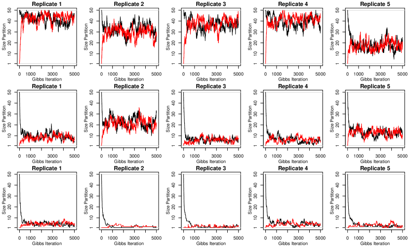
Figure 4: Trace plots of the sizes of partitions obtained from the Gibbs samplers for each of the five replicates (columns). We considered the logistic model in dimension $D=50$ with parameter $\theta=0.9,0.6,0.3$ (top to bottom rows). Initial partitions were taken as $\{\{1\},\ldots,\{D\}\}$ (black) and $\{\{1,\ldots,D\}\}$ (red). $5000$ iterations were performed.

In all cases, we can see that the Gibbs sampler converges rather quickly, and that it is enough to discard a burn-in of about $10\times D=500$ iterations.

To validate such results for another max-stable model, we did the same experiment for the Brown–Resnick model (Kabluchko et al., 2009), defined by taking $W_{j}(s)=\exp\{\varepsilon_{j}(s)-\gamma(s)\}$ in (9), where the terms $\varepsilon_{j}(s)$ are independent copies of $\varepsilon(s)$, which is an intrinsically stationary Gaussian process with zero mean and variogram $2\gamma(h)={\rm var}\{\varepsilon(s)-\varepsilon(s+h)\}$ such that $\varepsilon(0)=0$ almost surely. Using the exact simulation algorithm of Dombry et al. (2016), we simulated five independent replicates of the Brown–Resnick with semi-variogram $\gamma(h)=(h/\lambda)^{\nu}$, where $\lambda>0$ and $\nu\in(0,2]$ are the range and smoothness parameters, respectively, at $D=10$ randomly generated sites $s_{1},\ldots,s_{10}\in[0,1]^{2}$. We considered the cases $\lambda=0.5,1,1.5$ (short to long range dependence) with $\nu=1.5$. For each dataset, we ran five Gibbs samplers (one per independent replicate) for $1000$ iterations. Figure 5 shows the trace plots of the sizes of partitions along the different Markov chains. As before, the initial partitions were taken as $\{\{1\},\ldots,\{D\}\}$ (of size $D=10$) and $\{\{1,\ldots,D\}\}$ (of size one).

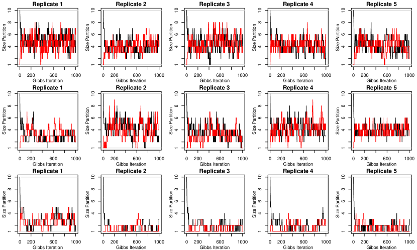
Figure 5: Trace plots of the sizes of partitions obtained from the Gibbs samplers for each of the five replicates (columns). We considered the Brown–Resnick model at $D=10$ sites in $[0,1]^{2}$ with semi-variogram $\gamma(h)=(h/\lambda)^{\nu}$ and parameters $\lambda=0.5,1,1.5$ (top to bottom rows) with $\nu=1.5$. Initial partitions were taken as $\{\{1\},\ldots,\{D\}\}$ (black) and $\{\{1,\ldots,D\}\}$ (red). $1000$ iterations were performed.

As concluded for the logistic model, we can see that the Gibbs sampler converges quickly and that about $10\times D=100$ iterations are enough for the algorithm to converge in all cases.

These results suggest to discard the first $10\times D$ iterations as burn-in, and to thin the resulting Markov chains by a factor $D$ to obtain approximately (conditionally) independent partitions. With this setting, the initial partition has negligible impact on the results. Alternatively, another natural option could be to initialize the partition randomly from its unconditional distribution, which can be easily obtained from an unconditional simulation of the max-stable distribution. This could potentially provide further computational savings by reducing the time it takes for the Gibbs sampler to converge (thus reducing the burn-in).

A.4 Simulation results for the Brown–Resnick model

We now provide further simulation results for the Brown–Resnick model. We follow the definition given in §A.3 using the semi-variogram $\gamma(h)=(h/\lambda)^{\nu}$, where $\lambda>0$ and $\nu\in(0,2]$ are the range and smoothness parameters, and we consider the scenarios displayed in Table 1. Realizations for each scenario are illustrated in Fig. 6.

Table 1: Scenarios considered for the simulation study based on the Brown–Resnick model with semi-variogram $\gamma(h)=(h/\lambda)^{\nu}$.

Scenarios (i.e., parameter configurations $\lambda;\nu$)
1	2	3	4	5	6	7	8	9
$0.5;0.5$	$0.5;1.0$	$0.5;1.5$	$1.0;0.5$	$1.0;1.0$	$1.0;1.5$	$1.5;0.5$	$1.5;1.0$	$1.5;1.5$

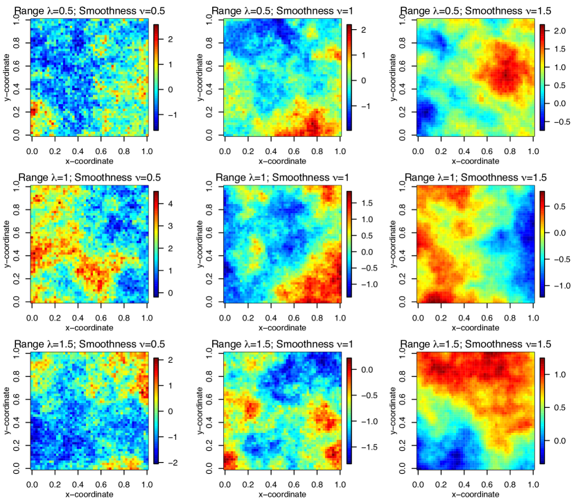
Figure 6: Realizations from the Brown–Resnick model on $[0,1]^{2}$, with semi-variogram $\gamma(h)=(h/\lambda)^{\nu}$, and parameter values taken according to Table 1, covering short to long range dependent processes (top to bottom) and rough to smooth processes (left to right). Realizations are displayed on standard Gumbel margins.

In order to assess the performance of the stochastic Expectation-Maximisation estimator in each scenario of Table 1, we simulated in each case $10$ independent copies of the Brown–Resnick model at $D=10$ randomly generated sites in $[0,1]^{2}$, and then estimated the range and smoothness parameters. We used (i) the stochastic Expectation-Maximisation estimator ${\widehat{\theta}}_{\rm SEM}=({\widehat{\lambda}}_{\rm SEM},{\widehat{\nu}}_{\rm SEM})^{{\mathrm{\scriptscriptstyle T}}}$ based on $60\times D=600$ Gibbs iterations in total, then thinning by a factor $D=10$, after discarding a burn-in of $10\times D=100$ iterations to follow the results of §A.3; and (ii) a pairwise likelihood estimator ${\widehat{\theta}}_{\rm PAIR}=({\widehat{\lambda}}_{\rm PAIR},{\widehat{\nu}}_{\rm PAIR})^{{\mathrm{\scriptscriptstyle T}}}$ (see, e.g., Padoan et al., 2010; Huser and Davison, 2013), which maximizes the pairwise likelihood constructed by combining the likelihood contributions from all ${10\choose 2}=45$ pairs of sites together with equal weight. We repeated this experiment $1024$ times to compute performance metrics, such as the root mean squared error of parameter estimates.

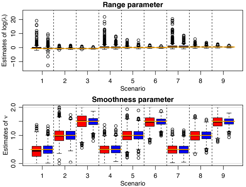
Figure 7: Boxplots of estimates of $\log(\lambda)$ (top) and $\nu$ (bottom) for each scenario in Table 1 based on the Brown–Resnick model with semi-variogram $\gamma(h)=(h/\lambda)^{\nu}$, simulated at $D=10$ random sites in $[0,1]^{2}$, with 10 independent replicates. Left (red) and right (blue) boxplots correspond to ${\widehat{\theta}}_{\rm PAIR}=({\widehat{\lambda}}_{\rm PAIR},{\widehat{\nu}}_{\rm PAIR})^{{\mathrm{\scriptscriptstyle T}}}$ and ${\widehat{\theta}}_{\rm SEM}=({\widehat{\lambda}}_{\rm SEM},{\widehat{\nu}}_{\rm SEM})^{{\mathrm{\scriptscriptstyle T}}}$, respectively. Each boxplot summarizes the variability of parameter estimates based on $1024$ simulations. Five estimates reaching up to $\log({\widehat{\lambda}}_{\rm PAIR})\approx 40$ were omitted in Scenario 1 for visibility purposes. Orange horizontal segments are the true values.

Figure 7 displays boxplots of estimated parameters for each scenario. Both stochastic Expectation-Maximisation and pairwise likelihood estimators seem to work well overall with a very low bias, although the variability is in some cases very high, due to the tricky estimation exercise with only $10$ replicates in dimension $D=10$. Nevertheless, the inter-quartile range appears to be quite moderate in all cases. The stochastic Expectation-Maximisation estimator appears clearly superior to the pairwise likelihood estimator in the cases we have considered, as it fully utilizes the information available in the data. To investigate this more in depth, Table 2 reports relative efficiencies of the pairwise likelihood estimator with respect to the stochastic Expectation-Maximisation estimator, defined as the ratio between the corresponding root mean squared errors (calculated from the 1024 replicates).

Table 2: Relative efficiencies ($\%$) for the estimates of $\log(\lambda)$ (left) and $\nu$ (right) based on the pairwise likelihood estimator with respect to the stochastic Expectation-Maximisation estimator. Simulations were based on the Brown–Resnick model with semi-variogram $\gamma(h)=(h/\lambda)^{\nu}$, simulated at $D=10$ random sites in $[0,1]^{2}$, with 10 independent replicates.

$\lambda/\nu$	$\nu=0.5$	$\nu=1.0$	$\nu=1.5$
$\lambda=0.5$	$39;75$	$94;80$	$77;59$
$\lambda=1.0$	$57;92$	$82;87$	$73;62$
$\lambda=1.5$	$54;92$	$79;82$	$71;61$

The results suggest that the stochastic Expectation-Maximisation estimator has a much better performance overall, as expected. Moreover, such results are expected to improve in higher-dimensional settings, where the loss in efficiency of pairwise likelihood estimators is more significant.

We now desire to check the speed of convergence of the Expectation-Maximisation algorithm, similarly to the simulations that we did for the logistic model in the main paper. Figure 8 displays the value of the likelihood (left panel) and the parameters (right panel) for each iteration $r=0,1,\ldots,20$ of the Expectation-Maximisation algorithm, for $100$ simulations performed in the exact same setting as above with true values chosen to be $\lambda=\nu=1.5$. The likelihood values were centred by their average over iterations 16–20 for visibility purposes. The plots show that the Expectation-Maximisation algorithm converges after roughly 5 iterations in this case, which is similar to the results obtained for the logistic model, recall the results in the main paper, despite the fact that the Brown–Resnick model has one more parameter ($p=2$). Hence, in practice, a small number of iterations could be chosen to speed up the algorithm.

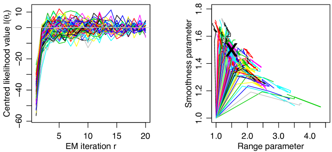
Figure 8: Left: likelihood value $l(\theta_{r})$ plotted as a function of the Expectation-Maximisation iteration $r=0,1,\ldots,20$, for $100$ simulations based on the Brown–Resnick model with semi-variogram $\gamma(h)=(h/\lambda)^{\nu}$, simulated at $D=10$ random sites in $[0,1]^{2}$, with 10 independent replicates. The likelihood values were centred by their average over iterations 16–20 for visibility purposes. Right: Trace of corresponding parameter values $\theta_{r}=(\lambda_{r},\nu_{r})^{{\mathrm{\scriptscriptstyle T}}}$, plotted for each Expectation-Maximisation iteration $r=0,1,\ldots,20$. The true values (black cross) are $\lambda=\nu=1.5$, while the initial values were taken to be $\lambda_{0}=\nu_{0}=1$.

The right panel of Fig. 8 also reveals that the estimated range parameter is negatively correlated with the estimated smoothness parameter. This was expected as these two parameters have an opposing effect on the dependence strength, and it suggests that alternative orthogonal parametrizations might be preferable. We leave this problem for future research.

Finally, we investigate the scalability of the stochastic Expectation-Maximisation estimator for the Brown–Resnick model when the dimension $D$ increases. To assess this, we considered the same setting as above with $10$ independent replicates, same number of Gibbs iterations, true values set to $\lambda=\nu=1.5$, and we measured the computational time needed for the first Expectation-Maximisation iteration, in dimensions $D=5,10,15,20$. Figure 9 plots the computational time on a logarithmic scale, along with a projection for dimensions up to $D=30$.

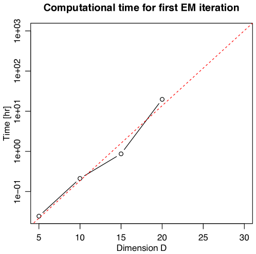
Figure 9: Computational time (hr) plotted on a logarithmic scale (black dots), for the first Expectation-Maximisation iteration. The values were obtained by averaging $1024$ computing times based on the Brown–Resnick model with semi-variogram $\gamma(h)=(h/\lambda)^{\nu}$, $\lambda=\nu=1.5$, simulated at $D=5,10,15,20$ random sites in $[0,1]^{2}$, with 10 independent replicates. The dashed red line represents a projection for higher dimensions, based on a linear fit (on logarithmic scale).

Unlike the logistic model, which has an explicit exponent function $V$ and partial derivatives $V_{\tau_{i}}$, the expressions for the Brown–Resnick model involve the multivariate Gaussian distribution in dimension up to $D-1$, whose computation is very demanding for large $D$. This significantly slows down the algorithm, whose complexity now appears to be increasing exponentially with $D$ (by contrast with the linear increase observed for the logistic model). More precisely, a single Expectation-Maximisation iteration takes on average approximately $1.5$min, $12.7$min, $52.2$min, and $19.8$hr for dimensions $D=5,10,15,20$, respectively. This precludes the use of the stochastic Expectation-Maximisation algorithm beyond dimension $D=20$, unless distributed computing resources are used to run all Gibbs sampler in parallel. Nevertheless, these results already represent a big advancement towards full likelihood inference for max-stable processes, as Castruccio et al. (2016) argued that a direct calculation of the likelihood was impossible beyond dimension $D=12$ or $13$. As shown by de Fondeville and Davison (2018), speed-ups can be obtained by appropriately exploiting quasi-Monte Carlo techniques for the calculation of multivariate Gaussian distributions. Alternatively, we could also use hierarchical matrix decompositions (Genton et al., 2018).

A similar computational burden is expected for the extremal-$t$ model (Opitz, 2013), which relies on the computation of multivariate Student $t$ distributions, but a better computational efficiency should prevail for the Reich and Shaby (2012) max-stable model, for which the expressions of the exponent function $V$ and its partial derivatives $V_{\tau_{i}}$ are available in explicit form; see the appendix of Castruccio et al. (2016).

References

- Booth and Hobert (1999) Booth, J. G. and Hobert, J. P. (1999) Maximizing generalized linear mixed model likelihoods with an automated Monte Carlo EM algorithm. J. R. Stat. Soc. Ser. B. Stat. Methodol. 61(1), 265–85.
- de Carvalho and Davison (2014) de Carvalho, M. and Davison, A. C. (2014) Spectral density ratio models for multivariate extremes. J. Amer. Statist. Assoc. 109(506), 764–76.
- Castruccio et al. (2016) Castruccio, S., Huser, R. and Genton, M. G. (2016) High-order composite likelihood inference for max-stable distributions and processes. J. Comput. Graph. Statist. 25, 1212–1229.
- Davis et al. (2013) Davis, R. A., Klüppelberg, C. and Steinkohl, C. (2013) Statistical inference for max-stable processes in space and time. J. R. Stat. Soc. Ser. B. Stat. Methodol. 75(5), 791–819.
- Davison and Huser (2015) Davison, A. C. and Huser, R. (2015) Statistics of extremes. Annu. Rev. Stat. Appl. 2, 203–35.
- Davison et al. (2013) Davison, A. C., Huser, R. and Thibaud, E. (2013) Geostatistics of dependent and asymptotically independent extremes. Math. Geosci. 45, 511–529.
- Davison et al. (2018) Davison, A. C., Huser, R. and Thibaud, E. (2018) Spatial extremes. In Handbook of Environmental and Ecological Statistics, eds A. E. Gelfand, M. Fuentes and R. L. Smith. CRC Press. To appear.
- Davison et al. (2012) Davison, A. C., Padoan, S. and Ribatet, M. (2012) Statistical modelling of spatial extremes (with discussion). Statist. Sci. 27(2), 161–86.
- Dempster et al. (1977) Dempster, A. P., Laird, N. M. and Rubin, D. B. (1977) Maximum likelihood from incomplete data via the EM algorithm. J. R. Stat. Soc. Ser. B. Stat. Methodol. 39(1), 1–38.
- Dombry et al. (2016) Dombry, C., Engelke, S. and Oesting, M. (2016) Exact simulation of max-stable processes. Biometrika 103(2), 303–17.
- Dombry et al. (2017a) Dombry, C., Engelke, S. and Oesting, M. (2017a) Bayesian inference for multivariate extreme value distributions. Electron. J. Statist. 11, 4813–4844.
- Dombry et al. (2017b) Dombry, C., Engelke, S. and Oesting, M. (2017b) Asymptotic properties of the maximum likelihood estimator for multivariate extreme value distributions. arXiv preprint 1612.05178.
- Dombry and Éyi-Minko (2013) Dombry, C. and Éyi-Minko, F. (2013) Regular conditional distributions of continuous max-infinitely divisible random fields. Electron. J. Probab. 18(7), 1–21.
- Dombry et al. (2013) Dombry, C., Éyi-Minko, F. and Ribatet, M. (2013) Conditional simulation of max-stable processes. Biometrika 100(1), 111–24.
- de Fondeville and Davison (2018) de Fondeville, R. and Davison, A. C. (2018) High-dimensional peaks-over-threshold inference. arXiv:1605.08558.
- Genton et al. (2018) Genton, M. G., Keyes, D. E. and Turkiyyah, G. (2018) Hierarchical decompositions for the computation of high-dimensional multivariate normal probabilities. Journal of Computational and Graphical Statistics 27, 268–277.
- Genton et al. (2011) Genton, M. G., Ma, Y. and Sang, H. (2011) On the likelihood function of Gaussian max-stable processes. Biometrika 98(2), 481–8.
- de Haan (1984) de Haan, L. (1984) A spectral representation for max-stable processes. Ann. Probab. 12(4), 1194–204.
- de Haan and Ferreira (2006) de Haan, L. and Ferreira, A. (2006) Extreme Value Theory: An Introduction. New York: Springer. ISBN 9780387239460.
- Huser and Davison (2013) Huser, R. and Davison, A. C. (2013) Composite likelihood estimation for the Brown–Resnick process. Biometrika 100(2), 511–8.
- Huser and Davison (2014) Huser, R. and Davison, A. C. (2014) Space-time modelling of extreme events. J. R. Stat. Soc. Ser. B. Stat. Methodol. 76(2), 439–61.
- Huser et al. (2016) Huser, R., Davison, A. C. and Genton, M. G. (2016) Likelihood estimators for multivariate extremes. Extremes 19(1), 79–103.
- Huser and Genton (2016) Huser, R. and Genton, M. G. (2016) Non-stationary dependence structures for spatial extremes. J. Agric. Biol. Environ. Stat. 21, 470–491.
- Kabluchko et al. (2009) Kabluchko, Z., Schlather, M. and de Haan, L. (2009) Stationary max-stable fields associated to negative definite functions. Ann. Probab. 37(5), 2042–65.
- Nielsen (2000) Nielsen, S. F. (2000) The stochastic EM algorithm: Estimation and asymptotic results. Bernoulli 6(3), 457–89.
- Opitz (2013) Opitz, T. (2013) Extremal processes: elliptical domain of attraction and a spectral representation. J. Multivariate Anal. 122(1), 409–13.
- Padoan et al. (2010) Padoan, S. A., Ribatet, M. and Sisson, S. A. (2010) Likelihood-based inference for max-stable processes. J. Amer. Statist. Assoc. 105(489), 263–77.
- Reich and Shaby (2012) Reich, B. J. and Shaby, B. A. (2012) A hierarchical max-stable spatial model for extreme precipitation. Ann. Appl. Stat. 6(4), 1430–51.
- Ribatet (2013) Ribatet, M. (2013) Spatial extremes: Max-stable processes at work. J. SFdS 154(2), 156–77.
- Sang and Genton (2014) Sang, H. and Genton, M. G. (2014) Tapered composite likelihood for spatial max-stable models. Spatial Statistics 8, 86–103.
- Schlather (2002) Schlather, M. (2002) Models for stationary max-stable random fields. Extremes 5(1), 33–44.
- Shi (1995) Shi, D. (1995) Fisher information for a multivariate extreme value distribution. Biometrika 82(3), 644–9.
- Smith (1990) Smith, R. L. (1990) Max-stable processes and spatial extremes. Unpublished.
- Stephenson and Tawn (2005) Stephenson, A. and Tawn, J. A. (2005) Exploiting occurrence times in likelihood inference for componentwise maxima. Biometrika 92(1), 213–27.
- Thibaud et al. (2016) Thibaud, E., Aalto, J., Cooley, D. S., Davison, A. C. and Heikkinen, J. (2016) Bayesian inference for the Brown–Resnick process, with an application to extreme low temperatures. Ann. Appl. Stat. 10, 2303–2324.
- Thibaud and Opitz (2015) Thibaud, E. and Opitz, T. (2015) Efficient inference and simulation for elliptical Pareto processes. Biometrika 102(4), 855–70.
- Varin et al. (2011) Varin, C., Reid, N. and Firth, D. (2011) An overview of composite likelihood methods. Statist. Sinica 21(2011), 5–42.
- Wadsworth (2015) Wadsworth, J. L. (2015) On the occurrence times of componentwise maxima and bias in likelihood inference for multivariate max-stable distributions. Biometrika 102(3), 705–11.
- Wadsworth and Tawn (2014) Wadsworth, J. L. and Tawn, J. A. (2014) Efficient inference for spatial extreme value processes associated to log-Gaussian random functions. Biometrika 101(1), 1–15.
- Xu and Genton (2016) Xu, G. and Genton, M. G. (2016) Tukey max-stable processes for spatial extremes. Spatial Statistics 18, 431–443.