Immersed boundary model of aortic heart valve dynamics with physiological driving and loading conditions

Abstract

The immersed boundary (IB) method is a mathematical and numerical framework for problems of fluid-structure interaction, treating the particular case in which an elastic structure is immersed in a viscous incompressible fluid. The IB approach to such problems is to describe the elasticity of the immersed structure in Lagrangian form, and to describe the momentum, viscosity, and incompressibility of the coupled fluid-structure system in Eulerian form. Interaction between Lagrangian and Eulerian variables is mediated by integral equations with Dirac delta function kernels. The IB method provides a unified formulation for fluid-structure interaction models involving both thin elastic boundaries and also thick viscoelastic bodies. In this work, we describe the application of an adaptive, staggered-grid version of the IB method to the three-dimensional simulation of the fluid dynamics of the aortic heart valve. Our model describes the thin leaflets of the aortic valve as immersed elastic boundaries, and describes the wall of the aortic root as a thick, semi-rigid elastic structure. A physiological left-ventricular pressure waveform is used to drive flow through the model valve, and dynamic pressure loading conditions are provided by a reduced (zero-dimensional) circulation model that has been fit to clinical data. We use this model and method to simulate aortic valve dynamics over multiple cardiac cycles. The model is shown to approach rapidly a periodic steady state in which physiological cardiac output is obtained at physiological pressures. These realistic flow rates are not specified in the model, however. Instead, they emerge from the fluid-structure interaction simulation.

1 Introduction

The immersed boundary (IB) method is a mathematical and numerical approach to problems of fluid-structure interaction that was introduced by Peskin to model the fluid dynamics of heart valves [1, 2]. The IB methodology has subsequently been used to model diverse problems in biological fluid dynamics [3] and other problems in which a rigid or elastic structure is immersed in a fluid flow [3, 4, 5]. The IB method for fluid-structure interaction treats problems in which an elastic structure is immersed in a viscous incompressible fluid, describing the elasticity of the immersed structure in Lagrangian form, and describing the momentum, viscosity, and incompressibility of the coupled fluid-structure system in Eulerian form. Integral equations with Dirac delta function kernels couple the Lagrangian and Eulerian variables. When discretized for computer simulation, the IB method approximates the Lagrangian equations on a curvilinear mesh, approximates the Eulerian equations on a Cartesian grid, and approximates the Lagrangian-Eulerian interaction equations by replacing the singular delta function with a regularized version of the delta function.

A key strength of the IB approach to fluid-structure interaction is that it does not require conforming Lagrangian and Eulerian discretizations. Specifically, the IB method permits the Lagrangian mesh to cut through the background Eulerian grid in an arbitrary manner and does not require dynamically generated body-fitted meshes. This attribute of the method greatly simplifies the task of grid generation and facilitates simulations involving large deformations of the elastic structure. An additional feature of the IB formulation is that it provides a unified approach to constructing models involving both thin elastic boundaries (i.e., immersed structures that are of codimension one with respect to the fluid) and also thick elastic bodies (i.e., immersed structures that are of codimension zero with respect to the fluid) [3].

In this work, we describe an adaptive version of the IB method and the application of this method to the simulation of the fluid dynamics of the aortic heart valve. Each year, approximately 250,000 procedures are performed to repair or replace damaged or destroyed heart valves [6]. Severe aortic valve disease is generally treated by replacement with either a mechanical or a bioprosthetic valve [7], and approximately 50,000 aortic valve replacements are performed annually to treat severe aortic stenosis [8, 9, 10]. Because many of the difficulties of prosthetic heart valves are related to the fluid dynamics of the replacement valve [6], mathematical and computational models that enable the study of the fluid-mechanical mechanisms of valve function and dysfunction may ultimately aid in improving treatment outcomes for the many patients suffering from valvular heart diseases.

The aortic valve model employed herein is similar, but not identical, to that described by Griffith et al. [11]. We model the thin leaflets of the aortic valve as immersed boundaries comprised of systems of elastic fibers that resist extension, compression, and bending, and we model the aortic root and ascending aorta as a thick, semi-rigid elastic structure. To construct the model valve leaflets, we use the mathematical theory of Peskin and McQueen [12], which describes the architecture of the systems of collagen fibers within the valve leaflets that allow the closed valve to support a significant pressure load. The geometry of the model aortic root is based on the idealized description of Reul et al. [13], which was derived from imaging data collected from healthy patients, and we use dimensions that are based on measurements by Swanson and Clark [14] of human aortic roots harvested after autopsy. A Windkessel model fit to human data by Stergiopulos et al. [15] provides physiological loading conditions for the model valve. Two limitations of our earlier model [11], which are overcome in the present work, are that it used only a highly idealized left-ventricular driving pressure waveform, and that it considered only a single cardiac cycle. In this work, we use a physiological driving pressure waveform that is based on human clinical data [16], and we perform multibeat simulations of the fluid dynamics of the aortic heart valve. We emphasize that we do not prescribe the flow rate at either the upstream or downstream boundaries of the model vessel. Instead, we impose a realistic, periodic left-ventricular driving pressure at the upstream boundary along with a dynamic circulatory loading pressure at the downstream boundary. With the driving and loading conditions used in the present work, our model rapidly approaches a periodic steady state in which physiological cardiac output is obtained at physiological pressures.

There are also important differences between the numerical methods used in the present study and those of our earlier simulations of aortic valve dynamics [11]. Although both use an adaptive version of the IB method for fluid-structure interaction, our earlier study used a cell-centered IB method [17], whereas herein we use a staggered-grid discretization. This is notable because we have recently demonstrated that staggered-grid IB methods yield substantially improved accuracy when compared to cell-centered discretizations [18]. Specifically, we have found that using a staggered-grid Eulerian discretization improves the volume-conservation properties of the IB method by one to two orders of magnitude in comparison to a cell-centered discretization [18]. Staggered-grid IB methods also yield improved resolution of pressure discontinuities [18]. In the present application, such discontinuities occur along the thin heart valve leaflets and are especially pronounced when the valve is closed and supporting a significant, physiological pressure load.

The three-dimensional adaptive IB method used in our simulations is similar to the two-dimensional adaptive IB method of Roma et al. [19]. Specifically, both schemes use a globally second-order accurate staggered-grid (i.e., marker-and-cell or MAC [20]) discretization of the incompressible Navier-Stokes equations on block-structured adaptively refined Cartesian grids, and both schemes implement formally second-order accurate versions of the IB method (i.e., schemes that yield second-order convergence rates for problems with sufficiently smooth solutions [21, 22]). There are also important differences between the present scheme and the scheme of Roma et al. For instance, the method of Roma et al. uses centered differencing to approximate the nonlinear advection terms of the incompressible Navier-Stokes equations, whereas we use a staggered-grid version [23] of the xsPPM7 variant [24] of the piecewise parabolic method (PPM) [25] that enables the application of the present method to high Reynolds number flows. Our scheme also uses the projection method not as a fractional-step solver for the incompressible Navier-Stokes equations, but rather as a preconditioner for an iterative Krylov method applied to an unsplit discretization of those equations [23]. Our approach eliminates the timestep-splitting error associated with standard projection methods. It also greatly simplifies the specification of physical boundary conditions along the outer boundaries of the computational domain. In this work, such physical boundary conditions couple the detailed, three-dimensional fluid-structure interaction model to the reduced circulation models that provide realistic driving and loading conditions.

2 The continuous equations of motion

The IB formulation of the equations of motion for a coupled fluid-structure system describes the elasticity of the immersed structure in Lagrangian form and describes the momentum, velocity, and incompressibility of the fluid-structure system in Eulerian form. Let $\bm{\mathrm{x}}=(x_{1},x_{2},x_{3})\in\Omega$ denote Cartesian physical coordinates, with $\Omega\subset\mathbb{R}^{3}$ denoting the physical region that is occupied by the fluid-structure system; let $\bm{\mathrm{s}}=(s_{1},s_{2},s_{3})\in U$ denote Lagrangian material coordinates that are attached to the immersed elastic structure, with $U\subset\mathbb{R}^{3}$ denoting the Lagrangian coordinate domain; and let $\bm{\mathrm{X}}(\bm{\mathrm{s}},t)\in\Omega$ denote the physical position of material point $\bm{\mathrm{s}}$ at time $t$. We consider the case in which the fluid possesses a uniform mass density $\rho$ and dynamic viscosity $\mu$, and we assume that the structure is neutrally buoyant and has the same viscous properties as the fluid in which it is immersed. These assumptions are not essential to the method, however, and generalizations of the IB method have been developed to permit the mass density of the structure to differ from that of the fluid [3, 26, 27, 28, 29, 30]. Work is also underway to develop new extensions of the IB method that permit the viscosity of the structure to differ from that of the fluid.

The IB formulation of the equations of fluid-structure interaction is [3]:

$$\rho\left(\frac{\partial\bm{\mathrm{u}}}{\partial t}(\bm{\mathrm{x}},t)+\bm{\mathrm{u}}(\bm{\mathrm{x}},t)\cdot\nabla\bm{\mathrm{u}}(\bm{\mathrm{x}},t)\right) =-\nabla p(\bm{\mathrm{x}},t)+\mu\nabla^{2}\bm{\mathrm{u}}(\bm{\mathrm{x}},t)+\bm{\mathrm{f}}(\bm{\mathrm{x}},t),$$ (1)

$$\nabla\cdot\bm{\mathrm{u}}(\bm{\mathrm{x}},t) =0,$$ (2)

$$\bm{\mathrm{f}}(\bm{\mathrm{x}},t) =\int_{U}\bm{\mathrm{F}}(\bm{\mathrm{s}},t)\,\delta(\bm{\mathrm{x}}-\bm{\mathrm{X}}(\bm{\mathrm{s}},t))\,{\rm d}\bm{\mathrm{s}},$$ (3)

$$\frac{\partial\bm{\mathrm{X}}}{\partial t}(\bm{\mathrm{s}},t) =\int_{\Omega}\bm{\mathrm{u}}(\bm{\mathrm{x}},t)\,\delta(\bm{\mathrm{x}}-\bm{\mathrm{X}}(\bm{\mathrm{s}},t))\,{\rm d}\bm{\mathrm{x}},$$ (4)

$$\bm{\mathrm{F}}(\bm{\mathrm{s}},t) =\bm{\mathrm{\mathcal{F}}}[\bm{\mathrm{X}}(\cdot,t)],$$ (5)

in which $\bm{\mathrm{u}}(\bm{\mathrm{x}},t)=(u_{1}(\bm{\mathrm{x}},t),u_{2}(\bm{\mathrm{x}},t),u_{3}(\bm{\mathrm{x}},t))$ is the Eulerian velocity field, $p(\bm{\mathrm{x}},t)$ is the Eulerian pressure, $\bm{\mathrm{f}}(\bm{\mathrm{x}},t)=(f_{1}(\bm{\mathrm{x}},t),f_{2}(\bm{\mathrm{x}},t),f_{3}(\bm{\mathrm{x}},t))$ is the Eulerian elastic force density (i.e., the elastic force density with respect to the physical coordinate system, so that $\bm{\mathrm{f}}(\bm{\mathrm{x}},t)\,{\rm d}\bm{\mathrm{x}}$ has units of force), $\bm{\mathrm{F}}(\bm{\mathrm{s}},t)=(F_{1}(\bm{\mathrm{s}},t),F_{2}(\bm{\mathrm{s}},t),F_{3}(\bm{\mathrm{s}},t))$ is the Lagrangian elastic force density (i.e., the elastic force density with respect to the material coordinate system, so that $\bm{\mathrm{F}}(\bm{\mathrm{s}},t)\,{\rm d}\bm{\mathrm{s}}$ has units of force), $\bm{\mathrm{\mathcal{F}}}:\bm{\mathrm{X}}\mapsto\bm{\mathrm{F}}$ is a functional that specifies the Lagrangian elastic force density in terms of the deformation of the immersed structure, and $\delta(\bm{\mathrm{x}})=\delta(x_{1})\,\delta(x_{2})\,\delta(x_{3})$ is the three-dimensional Dirac delta function. In this formulation, eqs. (3) and (4) are the interaction equations that couple the Lagrangian and Eulerian variables. Eq. (3) converts the Lagrangian force density $\bm{\mathrm{F}}(\bm{\mathrm{s}},t)$ into the equivalent Eulerian force density $\bm{\mathrm{f}}(\bm{\mathrm{x}},t)$. Eq. (4) states that the physical position of each Lagrangian material point $\bm{\mathrm{s}}$ moves with velocity $\bm{\mathrm{u}}(\bm{\mathrm{X}}(\bm{\mathrm{s}},t),t)$, thereby implying that there is no fluid slip at fluid-structure interfaces. Notice, however, that the no-slip condition of a viscous fluid does not appear in the equations as a constraint on the fluid motion. Instead, the no-slip condition determines the motion of the immersed structure. See, e.g., Peskin [3] for further discussion of these equations.

We next describe the form of the Lagrangian elastic force density functional $\bm{\mathrm{\mathcal{F}}}:\bm{\mathrm{X}}\mapsto\bm{\mathrm{F}}$ used in our model. Like our earlier study of cardiac valve dynamics [11], we model the flexible leaflets of the aortic valve as thin elastic boundaries, and we model the vessel wall as a thick, semi-rigid elastic structure. The elasticity of these structures is described in terms of families of fibers that resist extension, compression, and bending. We identify the model fibers of the valve leaflets with the collagen fibers that enable the real valve to support a significant pressure load when closed. In the case of the vessel wall, we do not identify the model fibers with particular physiological features; instead, these fibers are used simply to fix the geometry of the vessel.

As is frequently done in IB models [3], we define the fiber elasticity in terms of a strain-energy functional $E=E[\bm{\mathrm{X}}(\cdot,t)]$. The corresponding Lagrangian elastic force density may be expressed in terms of the Fréchet derivative of $E$. Specifically, $\bm{\mathrm{F}}$ is defined by

$$\bm{\mathrm{F}}=-\frac{\delta E}{\delta\bm{\mathrm{X}}},$$ (6)

which is shorthand for

$$\delta E[\bm{\mathrm{X}}(\cdot,t)]=-\int_{U}\bm{\mathrm{F}}(\bm{\mathrm{s}},t)\cdot\delta\bm{\mathrm{X}}(\bm{\mathrm{s}},t)\,{\rm d}\bm{\mathrm{s}}.$$ (7)

Notice that in eqs. (6) and (7), $\delta$ denotes the perturbation operator, not the Dirac delta function. To specify $E$, it is convenient to choose the Lagrangian coordinates $\bm{\mathrm{s}}=(s_{1},s_{2},s_{3})\in U$ so that each fixed value of $(s_{1},s_{2})$ labels a particular fiber. This implies that the mapping $s_{3}\mapsto\bm{\mathrm{X}}(s_{1}^{0},s_{2}^{0},s_{3})$ is a parametric representation of the fiber labeled by $(s_{1},s_{2})=(s_{1}^{0},s_{2}^{0})$. The curvilinear coordinate $s_{3}$ need not correspond to arc length along the fiber, however, and even if $s_{3}$ were to correspond to arc length in an initial or reference configuration, notice that it generally will not remain arc length as the structure deforms.

As we have done previously [11], we describe the total elastic energy functional $E$ as the sum of a stretching energy $E_{\text{s}}$ and a bending energy $E_{\text{b}}$, so that $E=E_{\text{s}}+E_{\text{b}}$. In turn, these elastic energy functionals determine a stretching force density $\bm{\mathrm{F}}_{\text{s}}$ and a bending force density $\bm{\mathrm{F}}_{\text{b}}$, so that $\bm{\mathrm{F}}=\bm{\mathrm{F}}_{\text{s}}+\bm{\mathrm{F}}_{\text{b}}$. The stretching energy is

$$E_{\text{s}}=\int_{\Omega}{\mathcal{E}}_{\text{s}}\left(\left|\frac{\partial\bm{\mathrm{X}}}{\partial s_{3}}\right|;\bm{\mathrm{s}}\right)\,{\rm d}\bm{\mathrm{s}},$$ (8)

in which ${\mathcal{E}}_{\text{s}}$ is a local stretching energy. The corresponding stretching force is given by [3]

$$\bm{\mathrm{F}}_{\text{s}}=\frac{\partial}{\partial s_{3}}\left({\mathcal{E}}_{\text{s}}^{\prime}\left(\left|\frac{\partial\bm{\mathrm{X}}}{\partial s_{3}}\right|;\bm{\mathrm{s}}\right)\frac{\partial\bm{\mathrm{X}}/\partial s_{3}}{\left|\partial\bm{\mathrm{X}}/\partial s_{3}\right|}\right),$$ (9)

in which ${\mathcal{E}}_{\text{s}}^{\prime}$ indicates the derivative of ${\mathcal{E}}_{\text{s}}$ with respect to its first argument. By identifying $T={\mathcal{E}}_{\text{s}}^{\prime}\left(\left|\partial\bm{\mathrm{X}}/\partial s_{3}\right|;\bm{\mathrm{s}}\right)$ as the fiber tension and $\bm{\mathrm{\tau}}=\partial\bm{\mathrm{X}}/\partial s_{3}/\left|\partial\bm{\mathrm{X}}/\partial s_{3}\right|$ as the fiber-aligned unit tangent vector, we may rewrite $\bm{\mathrm{F}}_{\text{s}}$ as

$$\bm{\mathrm{F}}_{\text{s}}=\frac{\partial}{\partial s_{3}}\left(T\bm{\mathrm{\tau}}\right).$$ (10)

The bending energy used in our model is

$$E_{\text{b}}=\frac{1}{2}\int_{\Omega}c_{\text{b}}(\bm{\mathrm{s}})\left|\frac{\partial^{2}\bm{\mathrm{X}}}{\partial s_{3}^{2}}-\frac{\partial^{2}\bar{\bm{\mathrm{X}}}}{\partial s_{3}^{2}}\right|^{2}\,{\rm d}\bm{\mathrm{s}},$$ (11)

in which $c_{\text{b}}=c_{\text{b}}(\bm{\mathrm{s}})$ is the spatially inhomogeneous bending stiffness, and $\bar{\bm{\mathrm{X}}}=\bar{\bm{\mathrm{X}}}(\bm{\mathrm{s}})$ is the reference configuration of the structure. The corresponding bending-resistant force is given by [11]

$$\bm{\mathrm{F}}_{\text{b}}=\frac{\partial^{2}}{\partial s_{3}^{2}}\left(c_{\text{b}}(\bm{\mathrm{s}})\left(\frac{\partial^{2}\bar{\bm{\mathrm{X}}}}{\partial s_{3}^{2}}-\frac{\partial^{2}\bm{\mathrm{X}}}{\partial s_{3}^{2}}\right)\right).$$ (12)

We take the reference configuration to be the initial configuration, i.e., $\bar{\bm{\mathrm{X}}}(\bm{\mathrm{s}})=\bm{\mathrm{X}}(\bm{\mathrm{s}},0)$. We remark that we use bending-resistant forces only within the model valve leaflets, i.e., $c_{\text{b}}(\bm{\mathrm{s}})\neq 0$ only for those fibers that comprise the valve leaflets. Because we model the valve leaflets as thin elastic surfaces immersed in fluid, including bending-resistant forces allows the model leaflets to account for the thickness of real valve leaflets, which are thin but, of course, not infinitely thin. In our model, we increase $c_{\text{b}}$ near the tips of the free edges of the valve leaflets to account for the fibrous noduli arantii.

Next, we specify the boundary conditions imposed along the outer boundary of the physical domain $\Omega$. We take $\Omega$ to be a $\mbox{10 cm}\times\mbox{10 cm}\times\mbox{15 cm}$ rectangular box, and we employ a combination of solid-wall and prescribed-pressure boundary conditions along $\partial\Omega$. Solid-wall boundary conditions are simply homogeneous Dirichlet conditions for the velocity field $\bm{\mathrm{u}}(\bm{\mathrm{x}},t)$. At solid-wall boundaries, a boundary condition for the pressure is neither needed nor permitted. By prescribed-pressure boundary conditions, we mean a combination of normal-traction and zero-tangential-slip boundary conditions. For a viscous incompressible fluid, it is easy to show that combining normal-traction and zero-tangential-slip boundary conditions along a flat boundary allows for the pointwise specification of the pressure $p(\bm{\mathrm{x}},t)$ on that boundary. To see this, recall that the Cauchy stress tensor of a viscous incompressible fluid is

$$\bm{\mathrm{\sigma}}=-p\mathbb{I}+\mu\left[\nabla\bm{\mathrm{u}}+\left(\nabla\bm{\mathrm{u}}\right)^{T}\right].$$ (13)

Let the outward unit normal at a position $\bm{\mathrm{x}}\in\partial\Omega$ be denoted by $\bm{\mathrm{n}}=\bm{\mathrm{n}}(\bm{\mathrm{x}})$, and let a unit tangent vector at a position $\bm{\mathrm{x}}\in\partial\Omega$ be denoted by $\bm{\mathrm{t}}=\bm{\mathrm{t}}(\bm{\mathrm{x}})$. By prescribing the normal traction at the boundary, we are prescribing the value of the normal component of the normal stress, i.e.,

$$\bm{\mathrm{n}}\cdot\bm{\mathrm{\sigma}}\cdot\bm{\mathrm{n}}=-p+2\mu\frac{\partial}{\partial n}(\bm{\mathrm{u}}\cdot\bm{\mathrm{n}}).$$ (14)

The zero-tangential-slip condition imposed on $\bm{\mathrm{u}}$ implies that $\bm{\mathrm{u}}\cdot\bm{\mathrm{t}}\equiv 0$ along $\partial\Omega$, and combining this condition with the incompressibility constraint implies that $\frac{\partial}{\partial n}(\bm{\mathrm{u}}\cdot\bm{\mathrm{n}})\equiv 0$ along $\partial\Omega$. Therefore, along $\partial\Omega$, the normal component of the normal stress reduces to

$$\bm{\mathrm{n}}\cdot\bm{\mathrm{\sigma}}\cdot\bm{\mathrm{n}}=-p.$$ (15)

Thus, combining normal-traction and zero-tangential-slip boundary conditions allows us to prescribe the value of the pressure pointwise along the boundary.

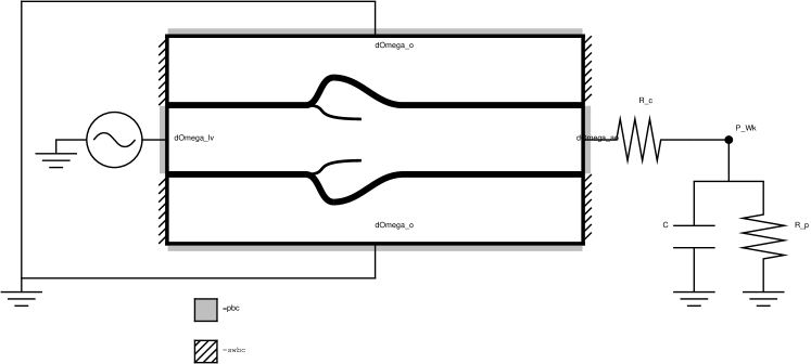
Figure 1: Schematic diagram of the model showing the coupling between the detailed fluid-structure interaction model and the reduced circulation models that provide physiological driving and loading conditions. The model vessel is coupled via the upstream boundary $\partial\Omega^{\text{LV}}$ to a prescribed left-ventricular pressure source that drives flow through the valve. At the downstream boundary $\partial\Omega^{\text{Ao}}$, the model vessel is coupled to a circulation model that provides a realistic pressure load. The open boundary $\partial\Omega^{\text{O}}$ provides a zero-pressure fluid reservoir that balances any changes in the volume of the vessel, which is modeled as a semi-rigid elastic structure.

The model vessel attaches directly to $\partial\Omega$, the outermost boundary of the physical domain. A schematic diagram is provided in fig. 1. Along $\partial\Omega^{\text{LV}}$, the upstream boundary of the vessel, a time-dependent left-ventricular pressure waveform $P^{\text{LV}}(t)$ is prescribed to drive flow through the model valve, so that

$$p(\bm{\mathrm{x}},t)=P^{\text{LV}}(t),\ \bm{\mathrm{x}}\in\partial\Omega^{\text{LV}}.$$ (16)

The specific left-ventricular pressure waveform used in the present model is adapted from the study of Murgo et al. [16]. The rate of flow entering the model vessel via the upstream boundary is

$$Q^{\text{LV}}(t)=-\int_{\partial\Omega^{\text{LV}}}\bm{\mathrm{u}}(\bm{\mathrm{x}},t)\cdot\bm{\mathrm{n}}\,{\rm d}a,$$ (17)

in which $\bm{\mathrm{n}}$ is the outward unit normal along $\partial\Omega$, and ${\rm d}a={\rm d}a(\bm{\mathrm{x}})$ is the area element in the Cartesian coordinate system.

On $\partial\Omega^{\text{Ao}}$, the downstream boundary of the vessel, we use a reduced (i.e., ordinary differential equation) circulation model to determine the pressure $P^{\text{Ao}}(t)$ that provides dynamic loading conditions for the model valve, so that

$$p(\bm{\mathrm{x}},t)=P^{\text{Ao}}(t),\ \bm{\mathrm{x}}\in\partial\Omega^{\text{Ao}}.$$ (18)

The reduced circulation model used in this work is a three-element Windkessel model with characteristic resistance $R_{\text{c}}$, peripheral resistance $R_{\text{p}}$, and arterial compliance $C$; see fig. 1. The rate of flow leaving the model vessel via the downstream boundary is

$$Q^{\text{Ao}}(t)=\int_{\partial\Omega^{\text{Ao}}}\bm{\mathrm{u}}(\bm{\mathrm{x}},t)\cdot\bm{\mathrm{n}}\,{\rm d}a.$$ (19)

Because we specify the pressure along $\partial\Omega^{\text{Ao}}$, the value of $Q^{\text{Ao}}(t)$ is not known in advance; instead, it must be determined by the coupled model. The flow leaving the fluid-structure interaction model via $\partial\Omega^{\text{Ao}}$ is exactly the flow through the circulation model, so that

$$\frac{1}{R_{\text{c}}}\left(P^{\text{Ao}}(t)-P^{\text{Wk}}(t)\right) =Q^{\text{Ao}}(t),$$ (20)

$$C\frac{\text{d}P^{\text{Wk}}}{\text{d}t}(t)+\frac{1}{R_{\text{p}}}P^{\text{Wk}}(t) =Q^{\text{Ao}}(t),$$ (21)

in which $P^{\text{Wk}}(t)$ is the stored pressure in the Windkessel model. Notice that the value of $P^{\text{Ao}}(t)$ is completely determined by $P^{\text{Wk}}(t)$ and $Q^{\text{Ao}}(t)$. In our simulations, we set $R_{\text{c}}=0.033$ (mmHg ml^-1 s), $R_{\text{p}}=0.79$ (mmHg ml^-1 s), and $C=1.75$ (ml mmHg^-1), corresponding to the human “Type A” beat characterized by Stergiopulos et al. [15].

Although we have found that coupling the detailed and reduced models via prescribed-pressure boundary conditions works well in practice, other choices of boundary conditions are possible. For instance, it is straightforward to devise boundary conditions for the incompressible Navier-Stokes equations that prescribe the mean pressure along a portion of a flat boundary; see ch. 3 sec. 8 of Gresho and Sani [31] for details. Alternatively, one may wish to couple the detailed and reduced models by prescribing boundary conditions for the normal component of the velocity. A drawback of this approach is that it would require determining an appropriate velocity profile at the boundary. A more serious limitation of this alternative approach is that prescribing the flow rate as a boundary condition, at either the upstream or the downstream boundary, makes it impossible to impose a realistic pressure difference across the model valve during the diastolic phase of the cardiac cycle. By using pressure boundary conditions at both the upstream and downstream boundaries of the vessel, we allow the normal component of the velocity profile at the boundary to be determined by the model, and we are able to impose realistic pressure loads on the model valve throughout the cardiac cycle.

Along $\partial\Omega^{\text{O}}$, the outermost portion of $\partial\Omega$ exterior to the model vessel, we set the pressure to equal zero. This external boundary condition provides an open boundary that acts to couple the fluid-structure interaction model to a zero-pressure fluid reservoir. This constant-pressure reservoir allows the vessel to change volume during the course of the simulation, i.e., it permits a mismatch between the instantaneous flow rates at the inflow and outflow boundaries of the vessel. Because we model the vessel wall as a semi-rigid elastic structure, we have that $Q^{\text{LV}}(t)\approx Q^{\text{Ao}}(t)$. Of course, once the model reaches periodic steady state, the time-integrated inflow and outflow volumes must match. The real aortic root is a flexible structure with significant compliance, however, and a model vessel that accounts for the physiological compliance of the aortic root would generally result in instantaneous differences between the inflow rate through $\partial\Omega^{\text{LV}}$ and the outflow rate through $\partial\Omega^{\text{Ao}}$.

All that remains is to specify the initial conditions. At time $t=0$, we set $\bm{\mathrm{u}}(\bm{\mathrm{x}},t)=0$ along with $P^{\text{LV}}(t)=P^{\text{Wk}}(t)=0$, so that all prescribed normal traction along the boundary are equal to zero. During a brief initialization period lasting 12.8 ms, we increase the left-ventricular driving pressure to a value of approximately 10 mmHg, and we increase the stored pressure in the Windkessel model to 85 mmHg, thereby establishing a realistic pressure load on the closed valve. During this initialization period, $P^{\text{Wk}}(t)$ is treated as a boundary condition and not as a state variable. That is to say, $P^{\text{Wk}}(t)$ does not satisfy eq. (21) for $t\leq\mbox{12.8 ms}$; rather, the value of $P^{\text{Wk}}(t)$ is prescribed. Once the model is initialized, however, $P^{\text{Wk}}(t)$ is treated as a state variable, the dynamics of which are determined by eq. (21).

3 The discrete equations of motion

3.1 Lagrangian and Eulerian spatial discretizations

As in our earlier simulation studies of cardiac fluid dynamics [11, 17], we discretize the Lagrangian equations on a fiber-aligned curvilinear mesh, and we discretize the Eulerian equations on a block-structured locally refined Cartesian grid that is adaptively generated to conform to the moving fiber mesh. The curvilinear mesh spacings are $\Delta s_{1}$, $\Delta s_{2}$, and $\Delta s_{3}$, and we use the indices $(l,m,n)$ to label the nodes of the Lagrangian mesh, so that $\bm{\mathrm{X}}_{l,m,n}$ and $\bm{\mathrm{F}}_{l,m,n}$ are the position and Lagrangian elastic force density associated with curvilinear mesh node $(l,m,n)$. The nodal values of $\bm{\mathrm{F}}_{l,m,n}$ are computed from the physical positions of the nodes of the curvilinear mesh via standard second-order accurate finite difference approximations to $\frac{\partial}{\partial s_{3}}$ and to $\frac{\partial^{2}}{\partial s_{3}^{2}}$. This approach is equivalent to describing the elasticity of the discretized model in terms of systems of springs and beams.

Figure 2: A two-dimensional locally refined hierarchical Cartesian grid comprised of two levels with refinement ratio ${\mathfrak{n}}=4$. Cartesian grid patch boundaries are indicated by bold lines. A single immersed fiber is embedded in level 1 of patch hierarchy. To simplify the discretization of the interaction equations that couple the Lagrangian and Eulerian variables, the Cartesian grid patches are constructed in a manner that ensures that the curvilinear mesh nodes are well separated from interfaces in Cartesian grid resolution.

The locally refined Cartesian grid is organized as a hierarchy of nested grid levels that are labeled $\ell=0,\ldots,\ell_{\text{max}}$, with $\ell=0$ denoting the coarsest level of the hierarchical grid and with $\ell=\ell_{\text{max}}$ denoting the finest level. Each grid level $\ell$ is comprised of the union of rectangular Cartesian grid patches. All grid patches in a given level $\ell$ of the grid hierarchy share the same uniform grid spacing $h^{\ell}$, and the grid spacings are chosen so that $h^{\ell}=h^{\ell-1}/{\mathfrak{n}}$, in which ${\mathfrak{n}}>\mbox{1}$ is an integer refinement ratio. The patch levels are constructed to satisfy the proper nesting condition [32], which generally requires that the union of the level $\ell+1$ grid patches be strictly contained within the union of the level $\ell$ grid patches. The proper nesting condition is relaxed at the outermost boundary of the physical domain, thereby allowing high Eulerian spatial resolution all the way up to $\partial\Omega$ in cases in which such resolution is needed. The patch levels are generated so that the faces of the grid patches that comprise level $\ell>0$ are coincident with the faces of the Cartesian grid cells that comprise level $\ell-1$, the next coarser level of the grid. This construction simplifies the development of composite-grid discretization methods that couple the levels of the locally refined grid. Except where noted, in our simulations, we employ a two-level adaptive grid, so that $\ell_{\text{max}}=1$, and we use ${\mathfrak{n}}=4$. An example two-dimensional grid is shown in fig. 2.

Figure 3: A two-dimensional locally refined staggered-grid discretization. The velocity field $\bm{\mathrm{u}}$ is approximated in terms of those vector components that are normal to the faces of the grid cells, and the pressure $p$ is approximated at the centers of the grid cells.

To discretize the Eulerian incompressible Navier-Stokes equations in space, we employ a locally refined version of a three-dimensional staggered-grid finite difference scheme; see fig. 3. The computational domain $\Omega$ is a rectangular box, $\Omega=[0,L_{1}]\times[0,L_{2}]\times[0,L_{3}]$, and the coarsest level of the locally refined Cartesian grid is a uniform discretization of $\Omega$, so that the union of the level $\ell=0$ grid patches form a regular $N_{1}\times N_{2}\times N_{3}$ Cartesian grid with grid spacings $\Delta x_{1}=\frac{L_{1}}{N_{1}}$, $\Delta x_{2}=\frac{L_{2}}{N_{2}}$, and $\Delta x_{3}=\frac{L_{3}}{N_{3}}$. For simplicity, we assume that $\Delta x_{1}=\Delta x_{2}=\Delta x_{3}=h^{0}$. On each level $\ell$ of the locally refined grid, $(i,j,k)$ labels a particular Cartesian grid cell, and $\bm{\mathrm{x}}_{i,j,k}=\mbox{$\left(\left(i+\frac{1}{2}\right)h^{\ell},\left(j+\frac{1}{2}\right)h^{\ell},\left(k+\frac{1}{2}\right)h^{\ell}\right)$}$ denotes the physical location of the center of that cell. The physical region covered by Cartesian grid cell $(i,j,k)$ on level $\ell$ is denoted by $\bm{\mathrm{c}}_{i,j,k}^{\ell}$, and the set of Cartesian grid cell indices associated with level $\ell$ is denoted by $\mathcal{G}^{\ell}$. The components of the Eulerian velocity field $\bm{\mathrm{u}}=(u_{1},u_{2},u_{3})$ are respectively approximated at the centers of the $x_{1}$, $x_{2}$, and $x_{3}$ faces of the Cartesian grid cells, i.e., at positions $\bm{\mathrm{x}}_{i-\frac{1}{2},j,k}=\mbox{$\left(ih^{\ell},\left(j+\frac{1}{2}\right)h^{\ell},\left(k+\frac{1}{2}\right)h^{\ell}\right)$}$, $\bm{\mathrm{x}}_{i,j-\frac{1}{2},k}=\mbox{$\left(\left(i+\frac{1}{2}\right)h^{\ell},jh^{\ell},\left(k+\frac{1}{2}\right)h^{\ell}\right)$}$, and $\bm{\mathrm{x}}_{i,j,k-\frac{1}{2}}=\mbox{$\left(\left(i+\frac{1}{2}\right)h^{\ell},\left(j+\frac{1}{2}\right)h^{\ell},kh^{\ell}\right)$}$. The pressure $p$ is approximated at the centers of the Cartesian grid cells. We use $(u_{1})_{i-\frac{1}{2},j,k}$, $(u_{2})_{i,j-\frac{1}{2},k}$, $(u_{3})_{i,j,k-\frac{1}{2}}$, and $p_{i,j,k}$ to denote the values of $\bm{\mathrm{u}}$ and $p$ that are stored on the grid. A staggered discretization is also used for the Eulerian body force $\bm{\mathrm{f}}=(f_{1},f_{2},f_{3})$, so that $f_{1}$, $f_{2}$, and $f_{3}$ are respectively approximated at the centers of the $x_{1}$, $x_{2}$, and $x_{3}$ faces of the Cartesian grid cells.

Let $\Omega^{\ell}\subseteq\Omega$ denote the physical region covered by the union of the level $\ell$ grid patches. By construction, $\Omega^{0}=\Omega$, and $\Omega^{\ell+1}\subseteq\Omega^{\ell}$. Moreover, away from $\partial\Omega$, $\Omega^{\ell+1}$ is strictly contained within $\Omega^{\ell}$. Notice that $\Omega^{\ell}=\cup_{(i,j,k)\in\mathcal{G}^{\ell}}\bm{\mathrm{c}}_{i,j,k}^{\ell}$. The coarse-fine interface between levels $\ell$ and $\ell+1$ is $\partial\Omega^{\ell+1}\setminus\partial\Omega^{\ell}$. Because the grid levels are constructed to satisfy the proper nesting condition, however, $\partial\Omega^{\ell+1}\cap\partial\Omega^{\ell}\subset\partial\Omega$, so that the coarse-fine interface between levels $\ell$ and $\ell+1$ is $\partial\Omega^{\ell+1}\setminus\partial\Omega$.

The refined region of level $\ell<\ell_{\text{max}}$, denoted by $\Omega^{\ell,\text{ref}}$, consists of the portion of $\Omega^{\ell}$ that is covered by $\Omega^{\ell+1}$, i.e., $\Omega^{\ell,\text{ref}}=\Omega^{\ell}\cap\Omega^{\ell+1}=\Omega^{\ell+1}$. The grid values of any quantity stored on the Cartesian grid that are physically located in $\Omega^{\ell,\text{ref}}$ are referred to as invalid values. The remaining values, i.e., those that are located in $\Omega^{\ell}\setminus\Omega^{\ell,\text{ref}}$, are referred to as valid values. The invalid values of level $\ell<\ell_{\text{max}}$ are constrained to be the restriction of the overlying level $\ell+1$ values. Notice that these overlying values could be either valid or invalid values, depending on the configuration of the grid hierarchy. The simplest restriction procedure is to define the coarse-grid invalid values to be the averages of the overlying fine-grid values; however, other restriction procedures are possible and, in fact, necessary to obtain higher-order accuracy at coarse-fine interfaces.

Each Cartesian grid patch is augmented by a layer of ghost cells that provide the values at the patch boundary that are needed to evaluate the approximations to the Eulerian spatial differential operators in the patch interior. We consider three types of ghost cells for the level $\ell$ grid patches: (1) ghost cells $(i,j,k)$ that overlap the interior of another level $\ell$ grid patch, so that $\bm{\mathrm{c}}_{i,j,k}^{\ell}\subset\Omega^{\ell}$; (2) ghost cells $(i,j,k)$ that overlap the interior of some level $\ell-1$ grid patch but not the interior of any of the level $\ell$ grid patches, so that $\bm{\mathrm{c}}_{i,j,k}^{\ell}\subset\Omega^{\ell-1}$ but $\bm{\mathrm{c}}_{i,j,k}^{\ell}\not\subset\Omega^{\ell}$; and (3) ghost cells that are exterior to $\Omega$, so that $\bm{\mathrm{c}}_{i,j,k}^{\ell}\not\subset\Omega$. For level $\ell$ ghost cells that overlap the interior of a neighboring level $\ell$-grid patch, the values in that ghost cell are simply copies of the neighboring interior values. If a level $\ell$ ghost cell overlaps the interior of a neighboring level $\ell-1$ grid patch but does not overlap the interior of any level $\ell$ grid patch, that ghost cell is said to be located on the coarse side of a coarse-fine interface. Ghost values located on the coarse side of a coarse-fine interface are defined by an interpolation procedure that uses both fine- and coarse-grid values. As we have done previously [11], we use a specialized quadratic interpolation procedure [33, 34, 35] to compute cell-centered ghost values at coarse-fine interfaces. For face-centered quantities, we use a generalization of this procedure that employs a combination of quadratic and cubic interpolation at coarse-fine interfaces. (Details of these coarse-fine interface discretizations are provided in the appendix.) Finally, ghost values that are exterior to the physical domain are determined via the physical boundary conditions in a manner that is analogous to the uniform-grid scheme for the incompressible Navier-Stokes equations of Griffith [23].

We denote by $\nabla_{h}\cdot\mbox{}\bm{\mathrm{u}}\approx\nabla\cdot\bm{\mathrm{u}}$, $\nabla_{h}p\approx\nabla p$, and $\nabla_{h}^{2}\bm{\mathrm{u}}\approx\nabla^{2}\bm{\mathrm{u}}$ composite-grid finite difference approximations to the divergence, gradient, and Laplace operators, respectively. We employ a standard staggered-grid (MAC) discretization approach, in which $\nabla_{h}\cdot\mbox{}\bm{\mathrm{u}}$ is computed at cell centers, whereas both $\nabla_{h}p$ and $\nabla_{h}^{2}\bm{\mathrm{u}}$ are computed on cell faces. Briefly stated, we use standard second-order accurate staggered-grid approximations to these operators within each Cartesian grid patch [23]. These uniform-grid patch-based discretizations are coupled to form composite-grid discretizations via restriction and prolongation operators. Although our composite-grid finite difference discretization of the incompressible Navier-Stokes equations is globally second-order accurate, this discretization does not retain the pointwise second-order accuracy of the basic uniform-grid approximation because of localized reductions in accuracy at coarse-fine interfaces.

To compute $\nabla_{h}\cdot\mbox{}\bm{\mathrm{u}}$ on the composite grid, we first use simple averaging to restrict $\bm{\mathrm{u}}$ from finer levels of the grid to coarser levels of the grid. We then compute for each level $\ell$ grid cell

$$\left(\nabla_{h}\cdot\mbox{}\bm{\mathrm{u}}\right)_{i,j,k}= \frac{\left(u_{1}\right)_{i+\frac{1}{2},j,k}-\left(u_{1}\right)_{i-\frac{1}{2},j,k}}{h^{\ell}}+\frac{\left(u_{2}\right)_{i,j+\frac{1}{2},k}-\left(u_{2}\right)_{i,j-\frac{1}{2},k}}{h^{\ell}}+\mbox{}$$

$$\frac{\left(u_{3}\right)_{i,j,k+\frac{1}{2}}-\left(u_{3}\right)_{i,j,k-\frac{1}{2}}}{h^{\ell}}.$$ (22)

To compute $\nabla_{h}p$ on the composite grid, we first use cubic interpolation to restrict $p$ from finer levels of the grid to coarser levels of the grid, and we then compute the composite-grid cell-centered interpolation of $p$ in the ghost cells along the coarse side of the coarse-fine interface. This approach ensures that the ghost values are at least third-order accurate interpolations of $p$. With the coarse-fine interface ghost values so determined, we then compute for each level $\ell$ cell face

$$(\nabla_{h}p)_{i-\frac{1}{2},j,k} =\frac{p_{i,j,k}-p_{i-1,j,k}}{h^{\ell}},$$ (23)

$$(\nabla_{h}p)_{i,j-\frac{1}{2},k} =\frac{p_{i,j,k}-p_{i,j-1,k}}{h^{\ell}},$$ (24)

$$(\nabla_{h}p)_{i,j,k-\frac{1}{2}} =\frac{p_{i,j,k}-p_{i,j,k-1}}{h^{\ell}}.$$ (25)

Finally, to compute $\nabla_{h}^{2}\bm{\mathrm{u}}$, we first use cubic interpolation to restrict $\bm{\mathrm{u}}$ from finer levels of the grid to coarser levels of the grid, and we then compute coarse-fine interface ghost values of $\bm{\mathrm{u}}$ using a composite-grid face-centered interpolation scheme, again ensuring that the ghost values are at least third-order accurate. We then compute for each $x_{1}$ face on level $\ell$

$$(\nabla_{h}^{2}u_{1})_{i-\frac{1}{2},j,k}= \frac{\left(u_{1}\right)_{i+\frac{1}{2},j,k}-2\left(u_{1}\right)_{i-\frac{1}{2},j,k}+\left(u_{1}\right)_{i-\frac{3}{2},j,k}}{\left(h^{\ell}\right)^{2}}+\mbox{}$$

$$\frac{\left(u_{1}\right)_{i-\frac{1}{2},j+1,k}-2\left(u_{1}\right)_{i-\frac{1}{2},j,k}+\left(u_{1}\right)_{i-\frac{1}{2},j-1,k}}{\left(h^{\ell}\right)^{2}}+\mbox{}$$

$$\frac{\left(u_{1}\right)_{i-\frac{1}{2},j,k+1}-2\left(u_{1}\right)_{i-\frac{1}{2},j,k}+\left(u_{1}\right)_{i-\frac{1}{2},j,k-1}}{\left(h^{\ell}\right)^{2}}.$$ (26)

Similar formulae are used to evaluate $\nabla_{h}^{2}u_{2}$ and $\nabla_{h}^{2}u_{3}$ on the $x_{2}$ and $x_{3}$ faces of the composite grid.

In the case of a uniform-grid discretization, notice that $\nabla_{h}\cdot\mbox{}\nabla_{h}$ is the usual 7-point cell-centered finite difference approximation to the Laplacian. This property facilities the construction of efficient preconditioners based on the projection method [23] and approximate Schur complement methods [36, 37]. In the presence of local mesh refinement, $\nabla_{h}\cdot\mbox{}\nabla_{h}$ is a relatively standard composite-grid generalization of the 7-point Laplacian [11, 17, 33, 34, 35] for which efficient solution algorithms, such as FAC (the fast adaptive composite-grid method) [38, 39, 40], have been developed.

3.2 Lagrangian-Eulerian interaction

To approximate the Lagrangian-Eulerian interaction equations, eqs. (3) and (4), we replace the delta function $\delta(\bm{\mathrm{x}})$ with a regularized version of the delta function $\delta_{h}(\bm{\mathrm{x}})$. The regularized delta function that we use is of the tensor-product form $\delta_{h}(\bm{\mathrm{x}})=\delta_{h}(x_{1})\,\delta_{h}(x_{2})\,\delta_{h}(x_{3})$, and we use a one-dimensional regularized delta function that is of the form $\delta_{h}(x)=\frac{1}{h}\phi\left(\frac{x}{h}\right)$. We take $\phi=\phi(r)$ to be the four-point delta function of Peskin [3].

We have found that fluid-structure interfaces generally require the highest available spatial resolution in an IB simulation. Therefore, we construct the Cartesian grid hierarchy so that the curvilinear mesh is embedded in the finest level of the grid. Additionally, because we use a regularized delta function with a support of four Cartesian meshwidths in each coordinate direction, we ensure that the locally refined grid is generated so that each curvilinear mesh point is physically located at least two level $\ell_{\text{max}}$ grid cells away from $\partial\Omega^{\ell_{\text{max}}}\setminus\partial\Omega$, the coarse-fine interface between levels $\ell_{\text{max}}-1$ and $\ell_{\text{max}}$. With these constraints on the configuration of the locally refined Cartesian grid, the nodes of the curvilinear mesh are directly coupled only to valid values defined on the finest level of the locally refined grid. This construction therefore allows us to discretize the Lagrangian-Eulerian interaction equations as if we were using a uniformly fine grid with resolution $h^{\ell_{\text{max}}}$.

With $\bm{\mathrm{f}}=(f_{1},f_{2},f_{3})$ and $\bm{\mathrm{F}}=(F_{1},F_{2},F_{3})$, we approximate eq. (3) componentwise by

$$(f_{1})_{i-\frac{1}{2},j,k} =\sum_{(l,m,n)}(F_{1})_{l,m,n}\,\delta_{h^{\ell_{\text{max}}}}(\bm{\mathrm{x}}_{i-\frac{1}{2},j,k}-\bm{\mathrm{X}}_{l,m,n})\,\Delta s_{1}\,\Delta s_{2}\,\Delta s_{3},$$ (27)

$$(f_{2})_{i,j-\frac{1}{2},k} =\sum_{(l,m,n)}(F_{2})_{l,m,n}\,\delta_{h^{\ell_{\text{max}}}}(\bm{\mathrm{x}}_{i,j-\frac{1}{2},k}-\bm{\mathrm{X}}_{l,m,n})\,\Delta s_{1}\,\Delta s_{2}\,\Delta s_{3},$$ (28)

$$(f_{3})_{i,j,k-\frac{1}{2}} =\sum_{(l,m,n)}(F_{3})_{l,m,n}\,\delta_{h^{\ell_{\text{max}}}}(\bm{\mathrm{x}}_{i,j,k-\frac{1}{2}}-\bm{\mathrm{X}}_{l,m,n})\,\Delta s_{1}\,\Delta s_{2}\,\Delta s_{3},$$ (29)

for $(i,j,k)\in\mathcal{G}^{\ell_{\text{max}}}$. The valid values of $\bm{\mathrm{f}}$ are set to equal zero on all coarser levels of the grid hierarchy. Similarly, with $\bm{\mathrm{u}}=(u_{1},u_{2},u_{3})$ and with $\bm{\mathrm{X}}=(X_{1},X_{2},X_{3})$, we approximate eq. (4) by

$$\frac{{\rm d}}{{\rm d}t}(X_{1})_{l,m,n} =\sum_{(i,j,k)\in\mathcal{G}^{\ell_{\text{max}}}}(u_{1})_{i-\frac{1}{2},j,k}\,\delta_{h^{\ell_{\text{max}}}}(\bm{\mathrm{x}}_{i-\frac{1}{2},j,k}-\bm{\mathrm{X}}_{l,m,n})\,\left(h^{\ell_{\text{max}}}\right)^{3},$$ (30)

$$\frac{{\rm d}}{{\rm d}t}(X_{2})_{l,m,n} =\sum_{(i,j,k)\in\mathcal{G}^{\ell_{\text{max}}}}(u_{2})_{i,j-\frac{1}{2},k}\,\delta_{h^{\ell_{\text{max}}}}(\bm{\mathrm{x}}_{i,j-\frac{1}{2},k}-\bm{\mathrm{X}}_{l,m,n})\,\left(h^{\ell_{\text{max}}}\right)^{3},$$ (31)

$$\frac{{\rm d}}{{\rm d}t}(X_{3})_{l,m,n} =\sum_{(i,j,k)\in\mathcal{G}^{\ell_{\text{max}}}}(u_{3})_{i,j,k-\frac{1}{2}}\,\delta_{h^{\ell_{\text{max}}}}(\bm{\mathrm{x}}_{i,j,k-\frac{1}{2}}-\bm{\mathrm{X}}_{l,m,n})\,\left(h^{\ell_{\text{max}}}\right)^{3},$$ (32)

in which we again consider only Cartesian grid cells on the finest level of the hierarchical grid. For those curvilinear mesh nodes that are in the vicinity of physical boundaries, we use the modified regularized delta function formulation of Griffith et al. [11]. This approach ensures that force and torque are conserved during Lagrangian-Eulerian interaction, even near $\partial\Omega$. To simplify the description of our timestepping algorithm, we use the shorthand $\bm{\mathrm{f}}=\bm{\mathrm{\mathcal{S}}}[\bm{\mathrm{X}}]\,\bm{\mathrm{F}}$ and $\frac{{\rm d}}{{\rm d}t}\bm{\mathrm{X}}=\bm{\mathrm{\mathcal{S}}}^{*}[\bm{\mathrm{X}}]\,\bm{\mathrm{u}}$, in which the force-spreading and velocity-interpolation operators, $\bm{\mathrm{\mathcal{S}}}[\bm{\mathrm{X}}]$ and $\bm{\mathrm{\mathcal{S}}}^{*}[\bm{\mathrm{X}}]$, are implicitly defined by eqs. (27)–(29) and (30)–(32), respectively.

3.3 Temporal discretization

We employ a simple timestep-splitting scheme to discretize the equations in time. Briefly, during each timestep, we first solve the fluid-structure interaction equations, treating the values of the upstream and downstream pressure boundary conditions as fixed. We then update the state variables of the circulation model, treating the fluid-structure interaction model state variables as fixed. This approach amounts to a first-order timestep splitting of the equations.

We discretize the fluid-structure interaction equations in time using truncated fixed-point iteration. We treat the linear terms in the incompressible Navier-Stokes equations implicitly, and we treat all other terms explicitly. Let $\bm{\mathrm{X}}^{n+1,k}$, $\bm{\mathrm{u}}^{n+1,k}$, and $p^{n+\frac{1}{2},k}$ denote the approximations to the values of $\bm{\mathrm{X}}$ and $\bm{\mathrm{u}}$ at time $t^{n+1}=(n+1)\Delta t$ and to the value of $p$ at time $t^{n+\frac{1}{2}}=(n+\frac{1}{2})\Delta t$ obtained after $k$ steps of fixed-point iteration, with $\bm{\mathrm{X}}^{n+1,0}=\bm{\mathrm{X}}^{n}$, $\bm{\mathrm{u}}^{n+1,0}=\bm{\mathrm{u}}^{n}$, and $p^{n+\frac{1}{2},0}=p^{n-\frac{1}{2}}$. Letting $\bm{\mathrm{X}}^{n+\frac{1}{2},k}=\frac{1}{2}\left(\bm{\mathrm{X}}^{n}+\bm{\mathrm{X}}^{n+1,k}\right)$ and $\bm{\mathrm{u}}^{n+\frac{1}{2},k}=\frac{1}{2}\left(\bm{\mathrm{u}}^{n}+\bm{\mathrm{u}}^{n+1,k}\right)$, we obtain $\bm{\mathrm{X}}^{n+1,k+1}$, $\bm{\mathrm{u}}^{n+1,k+1}$, and $p^{n+\frac{1}{2},k+1}$ by solving the linear system of equations

$$\rho\left(\frac{\bm{\mathrm{u}}^{n+1,k+1}-\bm{\mathrm{u}}^{n}}{\Delta t}+\bm{\mathrm{N}}^{n+\frac{1}{2},k}\right) =-\nabla_{h}p^{n+\frac{1}{2},k+1}+\mu\nabla_{h}^{2}\bm{\mathrm{u}}^{n+\frac{1}{2},k+1}+\bm{\mathrm{f}}^{n+\frac{1}{2},k},$$ (33)

$$\nabla_{h}\cdot\mbox{}\bm{\mathrm{u}}^{n+1,k+1} =0,$$ (34)

$$\bm{\mathrm{f}}^{n+\frac{1}{2},k} =\bm{\mathrm{\mathcal{S}}}[\bm{\mathrm{X}}^{n+\frac{1}{2},k}]\,\bm{\mathrm{F}}^{n+\frac{1}{2},k},$$ (35)

$$\frac{\bm{\mathrm{X}}^{n+1,k+1}-\bm{\mathrm{X}}^{n}}{\Delta t} =\bm{\mathrm{\mathcal{S}}}^{*}[\bm{\mathrm{X}}^{n+\frac{1}{2},k}]\,\bm{\mathrm{u}}^{n+\frac{1}{2},k+1},$$ (36)

$$\bm{\mathrm{F}}^{n+\frac{1}{2},k} =\bm{\mathrm{F}}_{\text{s}}[\bm{\mathrm{X}}^{n+\frac{1}{2},k}]+\bm{\mathrm{F}}_{\text{b}}[\bm{\mathrm{X}}^{n+\frac{1}{2},k}],$$ (37)

in which $\bm{\mathrm{N}}^{n+\frac{1}{2},k}\approx\left[\bm{\mathrm{u}}\cdot\nabla\bm{\mathrm{u}}\right]^{n+\frac{1}{2}}$ is an explicit approximation to the advection term that uses the xsPPM7 variant [24] of the piecewise parabolic method (PPM) [25] to discretize the nonlinear advection terms; see Griffith [23] for details. We use two cycles of fixed-point iteration per timestep to obtain a second-order accurate timestepping scheme. When solving for $\bm{\mathrm{X}}^{n+1,k+1}$, $\bm{\mathrm{u}}^{n+1,k+1}$, and $p^{n+\frac{1}{2},k+1}$, we fix the pressure at the upstream boundary $\partial\Omega^{\text{LV}}$ to be $p=P^{\text{LV}}(t^{n})$, and we fix the pressure at the downstream boundary $\partial\Omega^{\text{Ao}}$ to be $p=P^{\text{Ao}}(t^{n})$.

Next, having computed $\bm{\mathrm{X}}^{n+1}$, $\bm{\mathrm{u}}^{n+1}$, and $p^{n+\frac{1}{2}}$, we use $\bm{\mathrm{u}}^{n+1}$ to compute $Q^{\text{Ao}}\left(t^{n+1}\right)$, the instantaneous rate of flow leaving the vessel through $\partial\Omega^{\text{Ao}}$ at time $t^{n+1}$. We then update the value of $P^{\text{Wk}}$ via a second-order accurate explicit Runge-Kutta method, so that

$$C\frac{\tilde{P}^{\text{Wk}}\left(t^{n+1}\right)-P^{\text{Wk}}(t^{n})}{\Delta t}+\frac{1}{R_{\text{p}}}P^{\text{Wk}}\left(t^{n}\right) =Q^{\text{Ao}}\left(t^{n+1}\right),$$ (38)

$$C\frac{P^{\text{Wk}}\left(t^{n+1}\right)-P^{\text{Wk}}\left(t^{n}\right)}{\Delta t}+\frac{1}{R_{\text{p}}}\frac{\tilde{P}^{\text{Wk}}\left(t^{n+1}\right)+P^{\text{Wk}}\left(t^{n}\right)}{2} =Q^{\text{Ao}}\left(t^{n+1}\right).$$ (39)

We then set

$$P^{\text{Ao}}\left(t^{n+1}\right)=R_{\text{c}}Q^{\text{Ao}}\left(t^{n+1}\right)+P^{\text{Wk}}\left(t^{n+1}\right),$$ (40)

which serves as the downstream pressure boundary condition for the fluid-structure interaction model during the subsequent timestep. For the initial timestep, we set $P^{\text{LV}}(0)=P^{\text{Ao}}(0)=0$, values that are consistent with the initial conditions of the continuous system.

3.4 Cartesian grid adaptive mesh refinement

The locally refined grid is constructed in a recursive fashion: First, level 0 is constructed to cover the entire physical domain $\Omega$. Next, having constructed levels $0,\ldots,\ell<\ell_{\text{max}}$, level $\ell+1$ is generated by (1) tagging cells on level $\ell$ for refinement, (2) covering the tagged level $\ell$ grid cells by rectangular boxes generated by the Berger-Rigoutsos point-clustering algorithm [41], and (3) refining the generated boxes by the integer refinement ratio ${\mathfrak{n}}$ to form the level $\ell+1$ grid patches. Our cell-tagging criteria are simple rules that ensure that the immersed structure remains covered throughout the simulation by the grid cells that comprise the finest level of the hierarchical grid, and that attempt to ensure that flow features requiring enhanced resolution, such as vortices shed from the free edges of the valve leaflets, remain covered by grid cells of an appropriate resolution. Specifically, we tag grid cell $(i,j,k)$ on level $\ell<\ell_{\text{max}}$ for refinement whenever there exists some curvilinear mesh node $(l,m,n)$ such that $\bm{\mathrm{X}}_{l,m,n}\in\bm{\mathrm{c}}_{i,j,k}^{\ell}$, or whenever the local magnitude of the vorticity $\|\bm{\mathrm{\omega}}\|_{i,j,k}=\|\nabla_{h}\times\bm{\mathrm{u}}\|_{i,j,k}$ exceeds a relative threshold. Additional cells are added to the finest level of the grid to ensure that the coarse-fine interface between levels $\ell_{\text{max}}-1$ and $\ell_{\text{max}}$ is sufficiently far away from each of the curvilinear mesh nodes to prevent complicating the discretization of the Lagrangian-Eulerian interaction equations, as discussed previously. We emphasize that the positions of the curvilinear mesh nodes are not constrained to conform in any way to the locally refined Cartesian grid. Instead, the Cartesian grid patch hierarchy is adaptively updated to conform to the evolving configuration of the immersed elastic structure.

To prevent the immersed structure from “escaping” from the finest level of the grid, it is necessary to regenerate the locally refined grid at an interval that is determined by the CFL number of the flow. In our simulations, we choose the timestep size $\Delta t$ to satisfy a CFL condition of the form

$$\Delta t\leq\frac{1}{5}\min_{0\leq\ell\leq\ell_{\text{max}}}\min_{(i,j,k)\in\mathcal{G}^{\ell}}\frac{h^{\ell}}{\|\bm{\mathrm{u}}(\bm{\mathrm{x}}_{i,j,k})\|_{\infty}}.$$ (41)

This condition implies that each curvilinear mesh point moves at most $\frac{1}{5}$ fractional meshwidths per timestep. Therefore, to ensure that the immersed structure remains covered by $\Omega^{\ell_{\text{max}}}$, we must adaptively regenerate the grid hierarchy at least every five timesteps. In our simulations, we actually regenerate the grid every four timesteps. In practice, we could generally postpone regridding because the actual timestep size is generally smaller than that required by eq. (41) as a consequence of an additional stability restriction on $\Delta t$ that is of the form $\Delta t=O\left(\left(h^{\ell_{\text{max}}}\right)^{4}\right)$. This severe stability restriction results from our time-explicit treatment of the bending-resistant elastic force. For a model that includes only extension- and compression-resistant elastic elements, the stability restriction is reduced to $\Delta t=O\left(\left(h^{\ell_{\text{max}}}\right)^{2}\right)$.

Each time that the locally refined Cartesian grid is regenerated, Eulerian quantities must be transferred from the old grid hierarchy to the new one. In newly refined regions of the physical domain, the velocity field is prolonged from coarser levels of the old grid via a specialized conservative interpolation scheme that preserves the discrete divergence and curl of the staggered-grid velocity field [42]. (The basic divergence- and curl-preserving interpolation scheme [42] considers only the case in which ${\mathfrak{n}}=2$; however, this procedure is easily generalized to cases in which ${\mathfrak{n}}$ is a power of two via recursion.) The pressure, which is not a state variable of the system and which is used in the subsequent timestep only as an initial approximation to the updated pressure computed during that timestep (see below), is prolonged by simple linear interpolation. In newly coarsened regions of the domain, the values of the velocity and pressure are set to be the averages of the overlying fine-grid values from the old grid hierarchy.

4 Solution methodology

Solving for $\bm{\mathrm{X}}^{n+1,k+1}$, $\bm{\mathrm{u}}^{n+1,k+1}$, and $p^{n+\frac{1}{2},k+1}$ in eqs. (33)–(37) requires the solution of the linear system of equations,

$$\left(\begin{array}[]{cc}\frac{\rho}{\Delta t}I-\frac{\mu}{2}\nabla_{h}^{2}&\nabla_{h}\\ -\nabla_{h}\cdot\mbox{}&0\end{array}\right)\left(\begin{array}[]{c}\bm{\mathrm{u}}^{n+1,k+1}\\ p^{n+\frac{1}{2},k+1}\end{array}\right)=\left(\begin{array}[]{c}\left(\frac{\rho}{\Delta t}I+\frac{\mu}{2}\nabla_{h}^{2}\right)\bm{\mathrm{u}}^{n}-\rho\bm{\mathrm{N}}^{n+\frac{1}{2},k}+\bm{\mathrm{f}}^{n+\frac{1}{2},k}\\ 0\end{array}\right)$$ (42)

We solve eq. (42) via the FGMRES algorithm [43], using $\bm{\mathrm{u}}^{n+1,k}$ and $p^{n+\frac{1}{2},k}$ as initial approximations to $\bm{\mathrm{u}}^{n+1,k+1}$ and $p^{n+\frac{1}{2},k+1}$, and using the projection method as a preconditioner. (Recall that we define $\bm{\mathrm{u}}^{n+1,0}=\bm{\mathrm{u}}^{n}$ and $p^{n+\frac{1}{2},0}=p^{n-\frac{1}{2}}$.) Letting $A$ denote the matrix corresponding to this block system, i.e.,

$$A=\left(\begin{array}[]{cc}\frac{\rho}{\Delta t}I-\frac{\mu}{2}\nabla_{h}^{2}&\nabla_{h}\\ -\nabla_{h}\cdot\mbox{}&0\end{array}\right)$$ (43)

we write the corresponding projection method-based preconditioner matrix $B$ as [23]

$$B= \left(\begin{array}[]{cc}I&-\frac{\Delta t}{\rho}\nabla_{h}\\ 0&I-\frac{\Delta t}{\rho}\frac{\mu}{2}\nabla_{h}\cdot\mbox{}\nabla_{h}\end{array}\right)\left(\begin{array}[]{cc}I&0\\ 0&(\nabla_{h}\cdot\mbox{}\nabla_{h})^{-1}\end{array}\right)\cdot\mbox{}$$ (48)

$$\left(\begin{array}[]{cc}I&0\\ -\frac{\rho}{\Delta t}\nabla_{h}\cdot\mbox{}&-\frac{\rho}{\Delta t}I\end{array}\right)\left(\begin{array}[]{cc}\left(\frac{\rho}{\Delta t}I-\frac{\mu}{2}\nabla_{h}^{2}\right)^{-1}&0\\ 0&I\end{array}\right)$$ (53)

Because we use a preconditioned Krylov method to solve for $\bm{\mathrm{u}}^{n+1,k+1}$ and $p^{n+\frac{1}{2},k+1}$, it is not necessary to form explicitly the matrices corresponding to $A$ and $B$. Instead, we need only to be able to compute the application of these operators to arbitrary velocity- and pressure-like quantities. Computing the action of $A$ requires implementations of the finite difference approximations to the divergence, gradient, and Laplace operators described previously. Computing the action of $B$ additionally requires solvers for cell-centered and face-centered Poisson-type problems. It is not necessary, however, to employ exact solvers for these subdomain problems. In fact, these subdomain solvers may be quite approximate. At least in the present application, we have found that the performance of our implementation is optimized by using a single multigrid V-cycle of a cell-centered FAC preconditioner for the pressure subsystem, corresponding to the block $(\nabla_{h}\cdot\mbox{}\nabla_{h})^{-1}$ of the preconditioner $B$, and by applying two iterations of the conjugate gradient method for the velocity subsystem, corresponding to the block $\left(\frac{\rho}{\Delta t}I-\frac{\mu}{2}\nabla_{h}^{2}\right)^{-1}$ of the preconditioner. We are able to avoid using a multigrid method for the velocity subsystem because the Reynolds number of the flow is relatively large and the timestep size is relatively small, so that the linear system $\left(\frac{\rho}{\Delta t}I-\frac{\mu}{2}\nabla_{h}^{2}\right)$ is well conditioned.

We remark that although the projection method can be an extremely effective preconditioner [23], it does not appear to be widely used in this manner in practice. Instead, it is generally used as an approximate solver for the incompressible Navier-Stokes equations [34, 35, 44, 45, 46]. As a solver for the incompressible Navier-Stokes equations, the projection method is a fractional-step scheme that first solves the momentum equation over a time interval $[t^{n},t^{n+1}]$ for an “intermediate” velocity field without imposing the constraint of incompressibility, and then projects that intermediate velocity field onto the space of discretely divergence-free vector fields to obtain an approximation to the incompressible velocity field at time $t^{n+1}$. These two steps correspond to the two subdomain solves of our projection preconditioner, and each step requires the imposition of “artificial” physical boundary conditions. When the projection method is used as a solver, the artificial boundary conditions must be chosen carefully to yield a stable and accurate approximation to the true boundary conditions that are to be imposed on the coupled equations [46, 47]. Obtaining high-order accuracy may not be possible in all cases, such as for problems involving outflow boundaries [48], and constructing discretizations that are both stable and accurate can be difficult in practice [49].

We prefer to use the projection method as a preconditioner rather than as a solver. First, doing so permits the Krylov method to eliminate the timestep-splitting error of the basic projection method. Second, solving eq. (42), an unsplit discretization of the incompressible Stokes equations, permits us to impose directly the true boundary conditions on $\bm{\mathrm{u}}$ and $p$ in a coupled manner. Specifically, the form of the artificial boundary conditions required of the basic projection method does not affect the accuracy of the overall solver. This greatly simplifies the development of higher-order accurate discretiations of various types of boundary conditions. See Griffith [23] for details on the construction of accurate discretizations of various combinations of normal and tangential velocity and traction boundary conditions.

5 Implementation

Our adaptive IB method is implemented in the IBAMR software framework, a freely available C++ library for developing fluid-structure interaction models that use the IB method [50]. IBAMR provides support for distributed-memory parallelism via MPI and Cartesian grid adaptive mesh refinement. IBAMR relies upon the SAMRAI [51, 52, 53], PETSc [54, 55, 56], and hypre [57, 58] libraries for much of its functionality.

6 Computational results

6.1 Model results

A.			B.

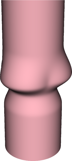
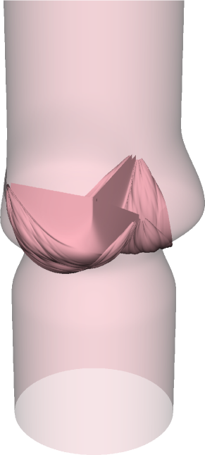
Figure 4: The initial configuration of the model aortic root and valve leaflets. In this and subsequent figures, the upstream boundary $\partial\Omega^{\text{LV}}$ is generally located at the bottom of each panel, and the downstream boundary $\partial\Omega^{\text{Ao}}$ is generally located at the top of each panel. A. The geometry of the model aortic root is based on the idealized description of Reul et al. [13], using dimensions based on measurements by Swanson and Clark [14]. B. The geometry and fiber architecture of the model aortic valve leaflets are determined by the mathematical theory of Peskin and McQueen [12].

A.
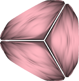
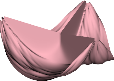
B.

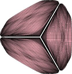
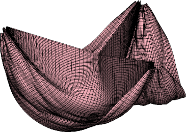
Figure 5: The model valve leaflets in their initial, loaded configuration. A. Surface renderings of the valve leaflets. B. Similar to A, but also showing a subset of the model fibers that comprise the leaflets.

Using the methods described herein, we have simulated the fluid dynamics of the aortic valve over multiple cardiac cycles, using a time-periodic left-ventricular driving pressure and dynamic loading conditions. In these simulations, the physical domain $\Omega$ is a $\mbox{10 cm}\times\mbox{10 cm}\times\mbox{15 cm}$ rectangular box that we discretize using a two-level adaptively refined Cartesian grid with refinement ratio ${\mathfrak{n}}=4$ between grid levels. The coarse-grid resolution is $h^{0}=\mbox{3.125 mm}$, which corresponds to that of a $32\times 32\times 48$ uniform discretization of $\Omega$, and the fine-grid resolution is $h^{1}=h^{\ell_{\text{max}}}=\mbox{0.78125 mm}$, which corresponds to that of a $128\times 128\times 192$ uniform discretization of $\Omega$. We model the valve leaflets as thin elastic surfaces because real aortic valve leaflets are only 0.2 mm thick [59], which is somewhat thinner than the Cartesian grid spacing on the finest level of the locally refined Cartesian grid. In contrast, we model the vessel as a thick elastic structure because the thickness of the aortic wall is 1 mm [60], which is relatively thick at the scale of the Cartesian grid. In our simulations, we use a uniform timestep size of $\Delta t=\mbox{6.25 $\mu$s}$, thereby requiring 128,000 timesteps per 0.8 s cardiac cycle. This value of $\Delta t$ was empirically determined to be approximately the largest stable timestep permitted by the present model and semi-explicit numerical method.

As discussed earlier, the elasticity of the valve leaflets and vessel wall is modeled using systems of fibers. In our model, each valve leaflet is spanned by two families of fibers. The first family of fibers runs from commissure to commissure, and the second family runs orthogonal to the commissural fibers. We view the commissural fibers as corresponding to the collagen fibers that allow the real valve leaflets to support a significant pressure load, and we use the mathematical theory of Peskin and McQueen [12] to determine the architecture of these fibers. We remark that the construction of Peskin and McQueen yields discretized fibers that form an orthogonal net, thereby facilitating the construction of the second family of fibers. Because this mathematical theory of the valve fiber architecture describes the geometry of the closed, loaded valve, we assume that the commissural fibers are initialized in a condition of 10% strain, and we choose the commissural fiber stiffness so that the closed valve supports a pressure load of approximately 80 mmHg. The second family of fibers is 10% as stiff as the commissural fibers, thereby approximating the anisotropic material properties of real aortic valve leaflets [61]. Notice that although the valve leaflets are initialized in a strained configuration, the boundary conditions at time $t=0$ do not provide the closed valve with any pressure load. This initial strain thereby induces oscillations in the valve leaflets, as if the valve had been struck like a drumhead at time $t=0$. These oscillations are rapidly damped by the viscosity of the fluid but nonetheless render the results of the first simulated beat somewhat atypical. The initial configuration of the model vessel and valve leaflets are shown in figs. 4 and 5.

The geometry of the aortic root and ascending aorta is based on the geometric description of Reul et al. [13], and the dimensions of the model vessel are based on measurements by Swanson and Clark of human aortic roots harvested post autopsy that were pressurized to 120 mmHg [14]. The stiffnesses of the fibers that comprise the vessel wall are empirically determined to keep the vessel essentially fixed in place. Our model therefore neglects the significant compliance of the real aortic root, which increases in volume by approximately 35% during ejection [62]. The incorporation of a realistic description of the elasticity of the aortic root and ascending aorta into our fluid-structure interaction model remains important future work.

A.

B. & \psfragscanon\psfrag{s05}[t][t]{\color[rgb]{0,0,0}\begin{tabular}[]{c}time (s)\end{tabular}}\psfrag{s06}[b][b]{\color[rgb]{0,0,0}\begin{tabular}[]{c}pressure (mmHg)\end{tabular}}\psfrag{s10}{\color[rgb]{0,0,0}\begin{tabular}[]{c}\end{tabular}}\psfrag{s11}{\color[rgb]{0,0,0}\begin{tabular}[]{c}\end{tabular}}\psfrag{s12}[l][l]{\color[rgb]{0,0,0}$P^{\text{Ao}}$}\psfrag{s13}[l][l]{\color[rgb]{0,0,0}$P^{\text{LV}}$}\psfrag{s14}[l][l]{\color[rgb]{0,0,0}$P^{\text{Ao}}$}\psfrag{x01}[t][t]{0}\psfrag{x02}[t][t]{0.5}\psfrag{x03}[t][t]{1}\psfrag{x04}[t][t]{1.5}\psfrag{x05}[t][t]{2}\psfrag{x06}[t][t]{2.5}\psfrag{v01}[r][r]{0}\psfrag{v02}[r][r]{20}\psfrag{v03}[r][r]{40}\psfrag{v04}[r][r]{60}\psfrag{v05}[r][r]{80}\psfrag{v06}[r][r]{100}\psfrag{v07}[r][r]{120}\includegraphics{figs/bc_pres.eps} C. \psfragscanon\psfrag{s05}[t][t]{\color[rgb]{0,0,0}\begin{tabular}[]{c}time (s)\end{tabular}}\psfrag{s06}[b][b]{\color[rgb]{0,0,0}\begin{tabular}[]{c}pressure (mmHg)\end{tabular}}\psfrag{s10}{\color[rgb]{0,0,0}\begin{tabular}[]{c}\end{tabular}}\psfrag{s11}{\color[rgb]{0,0,0}\begin{tabular}[]{c}\end{tabular}}\psfrag{s12}[l][l]{\color[rgb]{0,0,0}$P^{\text{Wk}}$}\psfrag{s13}[l][l]{\color[rgb]{0,0,0}$P^{\text{Ao}}$}\psfrag{s14}[l][l]{\color[rgb]{0,0,0}$P^{\text{Wk}}$}\psfrag{x01}[t][t]{0}\psfrag{x02}[t][t]{0.5}\psfrag{x03}[t][t]{1}\psfrag{x04}[t][t]{1.5}\psfrag{x05}[t][t]{2}\psfrag{x06}[t][t]{2.5}\psfrag{v01}[r][r]{60}\psfrag{v02}[r][r]{70}\psfrag{v03}[r][r]{80}\psfrag{v04}[r][r]{90}\psfrag{v05}[r][r]{100}\psfrag{v06}[r][r]{110}\psfrag{v07}[r][r]{120}\includegraphics{figs/wk_pres.eps}

Figure 6: Results from a multibeat simulation of aortic valve dynamics. The familiar S${}_{\text{2}}$ (“dup”) heart sound is clearly visible in the flow trace (panel A) and the aortic loading pressure (panels B and C). Notice that the model, which is driven by a periodic left-ventricular pressure waveform, rapidly approaches a periodic steady state. A. The flow rate through the valve as a function of time. Mean stroke volume is approximately 65 ml for both the second and the third beat, and the peak flow rate is approximately 420 ml s^-1. We emphasize that the flow rate is not specified in the model; rather, it emerges from the fluid-structure interaction simulation. B. The prescribed left-ventricular driving pressure $P^{\text{LV}}(t)$ and the computed loading aortic pressure $P^{\text{Ao}}(t)$. C. The pressures $P^{\text{Ao}}(t)$ and $P^{\text{Wk}}(t)$ determined by the coupled Windkessel model.

A.
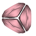
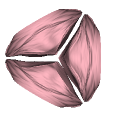
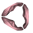
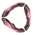
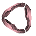
B.
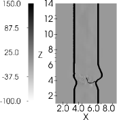
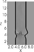
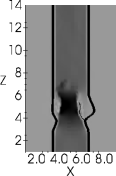
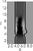
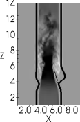
C.

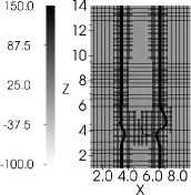
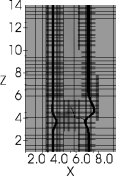
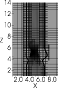
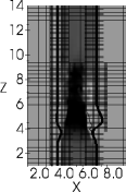
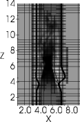
Figure 7: The opening dynamics of the valve during the second cardiac cycle, shown at equally spaced time intervals. A. The valve leaflets, as seen from the downstream boundary of the model. B. The model valve and vessel and the streamwise ($u_{3})$ component of the flow velocity along a plane that bisects one of the valve leaflets. C. Similar to B, but also showing the adaptively refined Cartesian grid.

A.
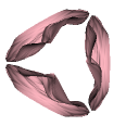
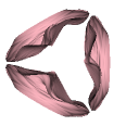
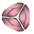
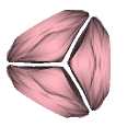
B.
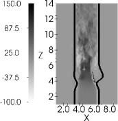
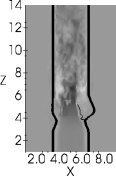
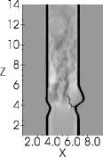
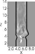
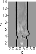
C.

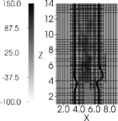
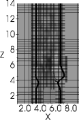
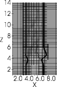
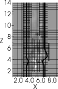
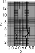
Figure 8: Similar to fig. 7, but here showing the closing dynamics of the valve during the second cardiac cycle. Notice that although there is minor regurgitation during valve closure, fig. 6.1A shows that once closed, the valve permits no further leak.

A.
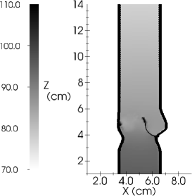
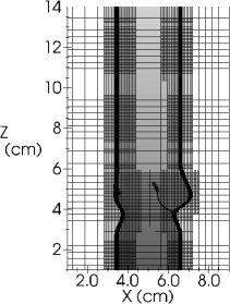
B.

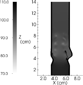
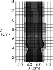
Figure 9: The configuration of the model valve and vessel, the pressure field, and, in the right panels, the locally refined Cartesian grid are shown along a plane that bisects one of the valve leaflets at (A) the time of maximum systolic pressure difference across the model valve and (B) the time of peak flow rate through the valve during the second simulated cardiac cycle. The maximum systolic pressure difference across the model valve, which is computed as the difference between the left ventricular pressure and the pressure approximately 1.5 cm downstream of the valve, is 12.2 mmHg during the second beat, and the pressure difference across the valve at the time of peak flow is 7.9 mmHg.

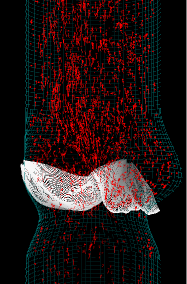
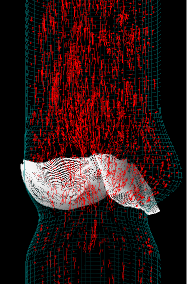
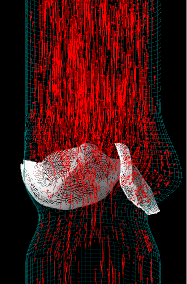
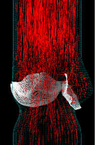
Figure 10: Flow through the model valve during valve opening as indicated by passively advected markers particles, shown at equally spaced time intervals.

Figs. 6.1–10 display representative results from a multibeat simulation using this model with left-ventricular driving pressures adapted from the human clinical data of Murgo et al. [16], and with loading conditions provided by the three-element Windkessel model of Stergiopulos et al. [15]. Recall that pressure boundary conditions are imposed at both the upstream and downstream boundaries of the model vessel. This is necessary to obtain a simulation in which the model valve supports a realistic pressure load during diastole. We remark that the realistic, nearly periodic flow rates produced by the model are not specified; instead, they emerge from the fluid-structure interaction simulation.

During the second and third beats of the simulation, mean stroke volume is approximately 65 ml, which is within the physiological range [63], whereas the peak flow rate is approximately 420 ml s^-1, which is somewhat lower than the peak flow rate reported by Murgo et al. [16]. Because the pressure field appears to be smoothly resolved in our simulation, we speculate that this difference is primarily related to the unphysiological rigidity of our vessel model and is not a consequence of numerical underresolution; however, this has not yet been demonstrated. The maximum systolic pressure difference across the model valve, which is computed as the difference between the left ventricular pressure and the pressure approximately 1.5 cm downstream of the valve, is 12.2 mmHg during the second beat and 12.0 mmHg during the third beat, values that are in good agreement with the corresponding experimentally obtained value of 12.8 mmHg reported by Driscol and Eckstein [64]. The pressure difference across the valve at the time of peak flow is 7.9 mmHg and 7.2 mmHg during the second and third beats, respectively. The mean transvalvular pressure difference of the model is 5.5 mmHg and 5.1 mmHg during the second and third beats, values that are somewhat higher than the experimental range of 1.2–2.9 mmHg [64]. Notice that the familiar S${}_{\text{2}}$ (“dup”) heart sounds, which correspond to the reverberations of the aortic valve leaflets upon the closure of the valve, are clearly visible in both the computed flow rate (fig. 6.1 panel A) and also the aortic loading pressure $P^{\text{Ao}}(t)$ (fig. 6.1 panels B and C).

6.2 Performance Analysis

	number of cores
	24	48	96
uniform grid	13.02	7.62	7.24
2-level grid	9.09	6.21	4.54
3-level grid	9.19	6.24	4.54

Table 1: Average wallclock time (in seconds) per timestep during the first 128 timesteps of the simulation for different numerical and computational parameters.

To gauge the computational performance of our adaptive method, we record the wallclock time required to perform the first 128 timesteps of the simulation. To obtain representative results, we average timings obtained for five successive runs of these first 128 timesteps. We compare the performance of the method when using a uniform Cartesian grid, a two-level Cartesian grid with refinement ratio ${\mathfrak{n}}=4$ between levels, and a three-level Cartesian grid with refinement ratio ${\mathfrak{n}}=4$ between levels. In all cases, the effective resolution of the finest level of the Cartesian grid hierarchy corresponds to that of a uniform $128\times 128\times 192$ grid. Timings were performed on the cardiac cluster at New York University, which is comprised of 80 Sun Microsystems, Inc., Sun Blade X8440 server modules interconnected by an InfiniBand network. Each compute server is equipped with four 2.3 GHz quad-core AMD Barcelona 8356 processors with 2 GB memory per core. We perform timings on two, four, or eight compute nodes, using four processors per node and three cores per processor for a total of 24, 48, or 96 cores per simulation. Timing results are summarized in table 1.

Notice that for the present model at the present effective fine-grid spatial resolution, the efficiency of the adaptive scheme is not improved by using a Cartesian grid hierarchy consisting of more than two levels. Specifically, when we use a three-level grid, most of the coarsest level is tagged for refinement and covered by the grid patches that comprise the next finer level of the grid hierarchy. Consequently, the total number of degrees of freedom is not reduced by an amount that is sufficient to overcome the increased computational overhead associated with the increased number of grid levels. In general, the optimal number of levels of refinement is problem dependent. For instance, by increasing the size of the physical domain $\Omega$ by a sufficient amount, it would eventually become computationally beneficial to use a Cartesian grid hierarchy comprised of three or more levels. Similarly, higher-resolution versions of the present aortic valve model would almost certainly benefit from additional levels of refinement. Because our semi-implicit timestepping scheme requires that $\Delta t=O\left(\left(h^{\ell_{\text{max}}}\right)^{4}\right)$ for problems involving bending-resistant elastic elements, however, it appears likely that a prerequisite for such a higher-resolution adaptive model is the development of an efficient implementation of an implicit version of this adaptive IB method.

7 Conclusions

In this work, we have described an adaptive, staggered-grid version of the IB method, and we have presented multibeat simulation results obtained by applying this method to a fluid-structure interaction model of the aortic heart valve that includes realistic driving and loading conditions. In our simulations, physiological flows are obtained with physiological pressure differences over multiple cardiac cycles. Only pressure boundary conditions are prescribed at the upstream and downstream boundaries of the model vessel. Nonetheless, realistic, time-periodic flow rates emerge from the coupled fluid-structure interaction model.

The primary differences between the simulations described herein and those of our earlier simulation study of cardiac valve dynamics [11] are that, in the present simulations, we use a physiological driving pressure waveform; we consider multiple cardiac cycles; and we employ an adaptive staggered-grid version of the IB method. The staggered-grid version of the IB method used in this work yields dramatic improvements in accuracy compared to our earlier cell-centered scheme [18], but despite these improvements in accuracy, work remains to obtain fully resolved simulations of the three-dimensional fluid dynamics of the aortic valve. Because of the severe restriction on the timestep size imposed by our semi-implicit timestepping scheme, however, it is difficult to deploy higher spatial resolution, even with the benefit of adaptive mesh refinement. We expect that obtaining higher-resolution IB simulations of aortic valve dynamics will require the development of an efficient parallel implementation of an implicit version of the IB method. Such methods promise to overcome the severe stability restrictions of semi-implicit IB methods, like that used in the present work, and we and others are actively working to develop efficient implicit IB methods.

Higher spatial resolution is not the only factor limiting the realism of our model. Another limitation of the present model is its simple description of the elasticity of the aortic valve and root. The present model could be improved by replacing these simple models with experimentally based constitutive models. Fiber-based elasticity models like those used in this work provide a convenient description of anisotropic structures commonly encountered in biological applications, and are well-suited for modeling the thin aortic valve leaflets, but combining realistic constitutive models with the fiber-based approach traditionally used with the IB method is difficult. The IB method is not restricted to fiber models, however, and several recent extensions of the IB method allow for more general elasticity models that permit finite element discretizations [65, 66, 67, 68, 69]. Using one such extension of the IB method [69], we aim to develop realistic IB models of aortic valve mechanics that will use experimentally characterized models of the aortic valve leaflets [70, 71, 72], the sinuses [73], and the ascending aorta [74], and to use such models to study the fluid dynamics of the aortic valve in both health and disease.

Appendix A Composite-Grid Discretization

Here, we provide additional details of the composite-grid finite difference discretizations used in the adaptive staggered-grid IB method. We use $(I,J,K)$ to index grid cells of a coarse level $\ell$ of the AMR grid hierarchy, and we use $(i,j,k)$ to index grid cells of the next finer level of the grid, level $\ell+1$. Throughout this appendix, $(i,j,k)=({\mathfrak{n}}I,{\mathfrak{n}}J,{\mathfrak{n}}K)$, i.e., fine grid cell $(i,j,k)$ and coarse grid cell $(I,J,K)$ share the vertex $\bm{\mathrm{x}}_{i-\frac{1}{2},j-\frac{1}{2},k-\frac{1}{2}}=\left(ih^{\ell+1},jh^{\ell+1},kh^{\ell+1}\right)=\left(Ih^{\ell},Jh^{\ell},Kh^{\ell}\right)=\bm{\mathrm{x}}_{I-\frac{1}{2},J-\frac{1}{2},K-\frac{1}{2}}$. We use the notation $u\!\left(I-\frac{1}{2},J,K\right)$, $v\!\left(I,J-\frac{1}{2},K\right)$, $w\!\left(I,J,K-\frac{1}{2}\right)$, and $p(I,J,K)$ to denote the values of $\bm{\mathrm{u}}=(u,v,w)$ and $p$ that are stored on the coarse level $\ell$ of the grid. Similar notation is used to denote values stored on the fine level $\ell+1$ of the grid.

A.1 Restriction

The composite-grid finite difference discretizations used in this work require a cell-centered cubic restriction procedure along with conservative and cubic face-centered restriction operators. To define these restriction procedures, we consider a single coarse grid cell $(I,J,K)$ on level $\ell$ along with the overlying ${\mathfrak{n}}\times{\mathfrak{n}}\times{\mathfrak{n}}$ grid cells on level $\ell+1$, namely grid cells $(i+\alpha,j+\beta,k+\gamma)$ for $\alpha,\beta,\gamma=0,\ldots,{\mathfrak{n}}-1$. Notice that

$$\bm{\mathrm{c}}_{I,J,K}^{\ell}=\bigcup_{\alpha,\beta,\gamma=0,\ldots,{\mathfrak{n}}-1}\bm{\mathrm{c}}_{i+\alpha,j+\beta,k+\gamma}^{\ell+1}.$$ (54)

A.1.1 Cell-centered cubic restriction

The cell-centered cubic restriction procedure, which requires ${\mathfrak{n}}$ to be even and at least four, defines a cell-centered quantity $p(I,J,K)$ on coarse level $\ell$ in terms of the closest overlying $4\times 4\times 4$ fine-grid values stored on level $\ell+1$ via

$$p(I,J,K):=\sum_{\alpha,\beta,\gamma=-2,\ldots,1}\omega(\alpha)\,\omega(\beta)\,\omega(\gamma)\,p\!\left(i+\frac{{\mathfrak{n}}}{2}+\alpha,j+\frac{{\mathfrak{n}}}{2}+\beta,k+\frac{{\mathfrak{n}}}{2}+\gamma\right),$$ (55)

in which $\omega(-2)=\omega(1)=-\frac{1}{16}$ and $\omega(-1)=\omega(0)=\frac{9}{16}$. In our implementation, if ${\mathfrak{n}}=2$, we revert to linear interpolation, which results in a reduction of the formal order of accuracy of our composite-grid discretization at coarse-fine interfaces. We do not permit ${\mathfrak{n}}$ to be odd because our recursive implementation of the divergence- and curl-preserving interpolation scheme [42] used to transfer the staggered-grid velocity field from one Cartesian grid hierarchy to another during adaptive regridding requires ${\mathfrak{n}}$ to be a power of two.

A.1.2 Face-centered conservative restriction

The face-centered conservative restriction procedure defines a face-centered quantity $\left(u\!\left(I-\frac{1}{2},J,K\right)\!,v\!\left(I,J-\frac{1}{2},K\right)\!,w\!\left(I,J,K-\frac{1}{2}\right)\right)$ on coarse level $\ell$ in terms of values stored in the overlying ${\mathfrak{n}}\times{\mathfrak{n}}\times{\mathfrak{n}}$ fine-grid cells on level $\ell+1$ via

$$u\!\left(I-\frac{1}{2},J,K\right) :=\frac{1}{{\mathfrak{n}}^{2}}\sum_{\beta,\gamma=0,\ldots,{\mathfrak{n}}-1}u\!\left(i-\frac{1}{2},j+\beta,k+\gamma\right),$$ (56)

$$v\!\left(I,J-\frac{1}{2},K\right) :=\frac{1}{{\mathfrak{n}}^{2}}\sum_{\alpha,\gamma=0,\ldots,{\mathfrak{n}}-1}v\!\left(i+\alpha,j-\frac{1}{2},k+\gamma\right),$$ (57)

$$w\!\left(I,J,K-\frac{1}{2}\right) :=\frac{1}{{\mathfrak{n}}^{2}}\sum_{\alpha,\beta=0,\ldots,{\mathfrak{n}}-1}w\!\left(i+\alpha,j+\beta,k-\frac{1}{2}\right).$$ (58)

This procedure is conservative in the sense of a finite volume scheme, i.e.,

$$u\!\left(I-\frac{1}{2},J,K\right)\left(h^{\ell}\right)^{2} =\sum_{\beta,\gamma=0,\ldots,{\mathfrak{n}}-1}u\!\left(i-\frac{1}{2},j+\beta,k+\gamma\right)\left(h^{\ell+1}\right)^{2},$$ (59)

$$v\!\left(I,J-\frac{1}{2},K\right)\left(h^{\ell}\right)^{2} =\sum_{\alpha,\gamma=0,\ldots,{\mathfrak{n}}-1}v\!\left(i+\alpha,j-\frac{1}{2},k+\gamma\right)\left(h^{\ell+1}\right)^{2},$$ (60)

$$w\!\left(I,J,K-\frac{1}{2}\right)\left(h^{\ell}\right)^{2} =\sum_{\alpha,\beta=0,\ldots,{\mathfrak{n}}-1}w\!\left(i+\alpha,j+\beta,k-\frac{1}{2}\right)\left(h^{\ell+1}\right)^{2}.$$ (61)

A.1.3 Face-centered cubic restriction

The face-centered cubic restriction procedure, which requires ${\mathfrak{n}}$ to be even and at least four, defines a face-centered quantity $u\!\left(I-\frac{1}{2},J,K\right)$ on coarse level $\ell$ in terms of the closest overlying $4\times 4$ fine-grid values stored on level $\ell+1$ via

$$u\!\left(I-\frac{1}{2},J,K\right):=\sum_{\beta,\gamma=-2,\ldots,1}\omega(\beta)\,\omega(\gamma)\,u\!\left(i-\frac{1}{2},j+\frac{{\mathfrak{n}}}{2}+\beta,k+\frac{{\mathfrak{n}}}{2}+\gamma\right),$$ (62)

in which $\omega(-2)=\omega(1)=-\frac{1}{16}$ and $\omega(-1)=\omega(0)=\frac{9}{16}$. Similar formulae define $v\!\left(I,J-\frac{1}{2},K\right)$ and $w\!\left(I,J,K-\frac{1}{2}\right)$. In our implementation, if ${\mathfrak{n}}=2$, we revert to linear interpolation, which results in a reduction of the formal order of accuracy of our composite-grid discretization at coarse-fine interfaces. We do not permit ${\mathfrak{n}}$ to be odd because our recursive implementation of the divergence- and curl-preserving interpolation scheme [42] used to transfer the staggered-grid velocity field from one Cartesian grid hierarchy to another during adaptive regridding requires ${\mathfrak{n}}$ to be a power of two.

A.2 Interpolation at coarse-fine interfaces

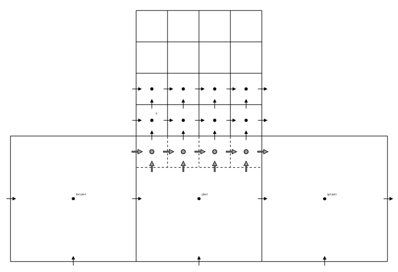
Figure 11: Two-dimensional grid configuration used to describe the coarse-fine interface interpolation scheme for cell- and face-centered quantities. In this configuration, a coarse level $\ell$ grid cell $(I,J-1)$ abuts ${\mathfrak{n}}=4$ fine level $\ell+1$ grid cells $(i+\alpha,j)$ for $\alpha=0,\ldots,{\mathfrak{n}}-1$. The coarse-fine interface ghost cells are indicated by dashed lines, and the values stored in these ghost cells are shown in gray with a black border. The cell- and face-centered quantities indicated in black are used to compute the ghost-cell values.

To describe the specialized interpolation scheme used to define values in the ghost cells abutting a coarse-fine interface, we temporarily restrict our discussion to two spatial dimensions. The extension of this interpolation scheme to three spatial dimensions is straightforward but difficult to visualize and cumbersome to describe, and therefore is not presented in detail.

We specifically consider the two-dimensional configuration shown in figs. 11–14, in which a coarse level $\ell$ grid cell $(I,J-1)$ abuts ${\mathfrak{n}}$ fine level $\ell+1$ grid cells $(i+\alpha,j)$ for $\alpha=0,\ldots,{\mathfrak{n}}-1$. (In the figures, as in our computations, we set ${\mathfrak{n}}=4$; however, the formulae presented in this subsection are valid for any even value of ${\mathfrak{n}}$. Different formulae would be required to treat the case in which ${\mathfrak{n}}$ is odd.) Formulae similar to those presented hold for other coarse-fine interface orientations. To define the values in the ghost cells located along this coarse-fine interface, we interpolate values stored in the coarse grid cells $(I+\alpha,J-1)$ for $\alpha=-1,0,1$ along with values stored in the two layers of fine grid cells that are adjacent to the coarse-fine interface, i.e., grid cells $(i+\alpha,j)$ and $(i+\alpha,j+1)$ for $\alpha=0,\ldots,{\mathfrak{n}}-1$. The values stored in coarse grid cells $(I-1,J-1)$ and $(I+1,J-1)$ may be either valid or invalid values, i.e., grid cells $(I-1,J-1)$ or $(I+1,J-1)$ could be located within the refined region of level $\ell$. If the values in coarse grid cells $(I-1,J-1)$ or $(I+1,J-1)$ are invalid values, those values are defined to be the cubic restriction of the overlying fine-grid values.

Our approach extends the cell-centered approach of Minion [33], Martin and Colella [34], and Martin et al. [35] to treat both cell-centered and face-centered quantities. We first interpolate coarse-grid values in the direction tangential to the coarse-fine interface, so as to obtain interpolated values at locations that are aligned with the valid fine-grid values. We then define the values in the ghost cells by interpolating in the direction normal to the coarse-fine interface, using the interpolated coarse-grid values along with the valid fine-grid values.

A.2.1 Cell-centered coarse-fine interpolation

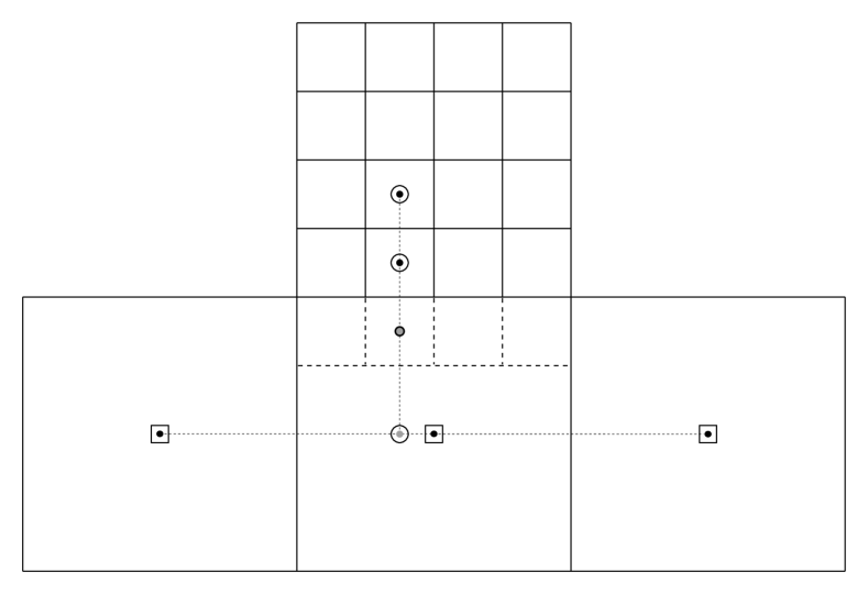
Figure 12: Cell-centered coarse-fine interface interpolation. First, an intermediate interpolated value, indicated in gray, is defined via quadratic interpolation in the direction tangential to the coarse-fine interface. The coarse-grid values that are used in this initial interpolation step are indicated by black boxes. Notice that the intermediate quantity is aligned with the fine-grid values, whereas the original coarse-grid values are not. Second, the coarse-fine interface ghost-cell value is defined via quadratic interpolation in the direction normal to the coarse-fine interface. The values that are used in this second interpolation step are indicated by black circles.

In reference to fig. 11, the cell-centered quantities that we wish to compute are denoted $p(i+\alpha,j-1)$, $\alpha=0,\ldots,{\mathfrak{n}}-1$. To define these values, we first compute intermediate values that are defined by performing quadratic interpolation in the direction tangential to the coarse-fine interface, using the coarse-grid values $p(I-1,J-1)$, $p(I,J-1)$, and $p(I+1,J-1)$. Specifically, we compute

$$p\!\left(i+\alpha,j-\frac{{\mathfrak{n}}+1}{2}\right) :=\frac{\left(2(i+\alpha)+1-{\mathfrak{n}}\right)\left(2(i+\alpha)+1-3{\mathfrak{n}}\right)}{8{\mathfrak{n}}^{2}}p(I-1,J-1)$$

$$\quad\mbox{}-\frac{\left(2(i+\alpha)+1+{\mathfrak{n}}\right)\left(2(i+\alpha)+1-3{\mathfrak{n}}\right)}{4{\mathfrak{n}}^{2}}p(I,J-1)$$

$$\quad\mbox{}+\frac{\left(2(i+\alpha)+1+{\mathfrak{n}}\right)\left(2(i+\alpha)+1-{\mathfrak{n}}\right)}{8{\mathfrak{n}}^{2}}p(I+1,J-1)$$ (63)

for $\alpha=0,\ldots,{\mathfrak{n}}-1$.

We then compute $p(i+\alpha,j-1)$, $\alpha=0,\ldots,{\mathfrak{n}}-1$, by performing quadratic interpolation in the direction normal to the coarse-fine interface, using the fine-grid values $p(i+\alpha,j)$ and $p(i+\alpha,j+1)$ along with the intermediate interpolated values. Specifically, we compute

$$p(i+\alpha,j-1) :=\frac{2({\mathfrak{n}}-1)}{1+{\mathfrak{n}}}p(i+\alpha,j)-\frac{{\mathfrak{n}}-1}{3+{\mathfrak{n}}}p(i+\alpha,j+1)$$

$$\quad\mbox{}+\frac{8}{(1+{\mathfrak{n}})(3+{\mathfrak{n}})}p\!\left(i+\alpha,j-\frac{{\mathfrak{n}}+1}{2}\right)$$ (64)

for $\alpha=0,\ldots,{\mathfrak{n}}-1$.

This two-step interpolation procedure is summarized in fig. 12 for ${\mathfrak{n}}=4$ and $\alpha=1$.

A.2.2 Face-centered coarse-fine interpolation of components normal to the coarse-fine interface

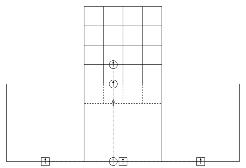
Figure 13: Face-centered coarse-fine interface interpolation of components normal to the coarse-fine interface. First, an intermediate interpolated value, indicated in gray, is defined via quadratic interpolation in the direction tangential to the coarse-fine interface. The coarse-grid values that are used in this initial interpolation step are indicated by black boxes. Second, the coarse-fine interface ghost-cell value is defined via quadratic interpolation in the direction normal to the coarse-fine interface. The values that are used in this second interpolation step are indicated by black circles.

The components of the staggered-grid velocity field that are normal to the coarse-fine interface are treated in a manner that is similar to the cell-centered coarse-fine interface interpolation scheme described in sec. A.2.1. In reference to fig. 11, the face-centered quantities that we wish to compute are denoted $v\!\left(i+\alpha,j-\frac{3}{2}\right)$, $\alpha=0,\ldots,{\mathfrak{n}}-1$. To define these values, we first compute intermediate values that are defined by performing quadratic interpolation in the direction tangential to the coarse-fine interface, using the coarse-grid values $v\!\left(I-1,J-\frac{3}{2}\right)$, $v\!\left(I,J-\frac{3}{2}\right)$, and $v\!\left(I+1,J-\frac{3}{2}\right)$. Specifically, we compute

$$v\!\left(i+\alpha,j-{\mathfrak{n}}-\frac{1}{2}\right) :=\frac{\left(2(i+\alpha)+1-{\mathfrak{n}}\right)\left(2(i+\alpha)+1-3{\mathfrak{n}}\right)}{8{\mathfrak{n}}^{2}}v\!\left(I-1,J-\frac{3}{2}\right)$$

$$\quad\mbox{}-\frac{\left(2(i+\alpha)+1+{\mathfrak{n}}\right)\left(2(i+\alpha)+1-3{\mathfrak{n}}\right)}{4{\mathfrak{n}}^{2}}v\!\left(I,J-\frac{3}{2}\right)$$

$$\quad\mbox{}+\frac{\left(2(i+\alpha)+1+{\mathfrak{n}}\right)\left(2(i+\alpha)+1-{\mathfrak{n}}\right)}{8{\mathfrak{n}}^{2}}v\!\left(I+1,J-\frac{3}{2}\right)$$ (65)

for $\alpha=0,\ldots,{\mathfrak{n}}-1$.

We then compute $v\!\left(i+\alpha,j-\frac{3}{2}\right)$, $\alpha=0,\ldots,{\mathfrak{n}}-1$, by performing quadratic interpolation in the direction normal to the coarse-fine interface, using the fine-grid values $v\!\left(i+\alpha,j-\frac{1}{2}\right)$ and $v\!\left(i+\alpha,j+\frac{1}{2}\right)$ along with the intermediate interpolated values. Specifically, we compute

$$v\!\left(i+\alpha,j-\frac{3}{2}\right) :=\frac{2({\mathfrak{n}}-1)}{{\mathfrak{n}}}v\!\left(i+\alpha,j-\frac{1}{2}\right)-\frac{{\mathfrak{n}}-1}{1+{\mathfrak{n}}}v\!\left(i+\alpha,j+\frac{1}{2}\right)$$

$$\quad\mbox{}+\frac{2}{{\mathfrak{n}}(1+{\mathfrak{n}})}v\!\left(i+\alpha,j-{\mathfrak{n}}-\frac{1}{2}\right)$$ (66)

for $\alpha=0,\ldots,{\mathfrak{n}}-1$.

This two-step interpolation procedure is summarized in fig. 13 for ${\mathfrak{n}}=4$ and $\alpha=1$.

A.2.3 Face-centered coarse-fine interpolation of components tangential to the coarse-fine interface

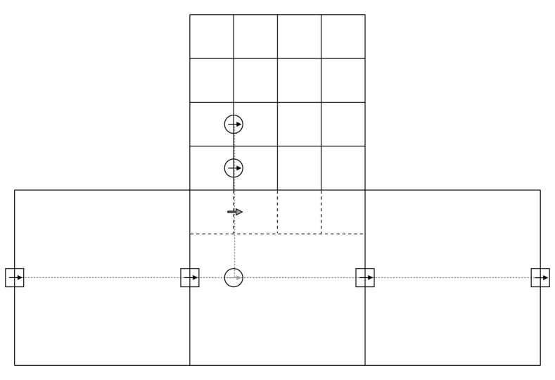
Figure 14: Face-centered coarse-fine interface interpolation of components tangential to the coarse-fine interface. First, an intermediate interpolated value, indicated in gray, is defined via cubic interpolation in the direction tangential to the coarse-fine interface. The coarse-grid values that are used in this initial interpolation step are indicated by black boxes. Second, the coarse-fine interface ghost-cell value is defined via quadratic interpolation in the direction normal to the coarse-fine interface. The values that are used in this second interpolation step are indicated by black circles.

The components of the staggered-grid velocity field that are tangential to the coarse-fine interface are treated in a manner that is similar to the interpolation schemes described in secs. A.2.1 and A.2.2, except that in this case, we perform cubic interpolation in the tangential direction instead of quadratic interpolation. In reference to fig. 11, the face-centered quantities that we wish to compute are denoted $u\!\left(i+\alpha-\frac{1}{2},j-1\right)$, $\alpha=0,\ldots,{\mathfrak{n}}$. To define these values, we first compute intermediate values that are defined by performing cubic interpolation in the direction tangential to the coarse-fine interface, using the coarse-grid values $u\!\left(I-\frac{3}{2},J-1\right)$, $u\!\left(I-\frac{1}{2},J-1\right)$, $u\!\left(I+\frac{1}{2},J-1\right)$, and $u\!\left(I+\frac{3}{2},J-1\right)$. Specifically, we compute

$$u\!\left(i+\alpha-\frac{1}{2},j-\frac{{\mathfrak{n}}+1}{2}\right) :=-\frac{(i+\alpha)\left(i+\alpha-{\mathfrak{n}}\right)\left(i+\alpha-2{\mathfrak{n}}\right)}{6{\mathfrak{n}}^{3}}u\!\left(I-\frac{3}{2},J-1\right)$$

$$\quad\mbox{}+\frac{\left(i+\alpha-{\mathfrak{n}}\right)\left(i+\alpha-2{\mathfrak{n}}\right)\left(i+\alpha+{\mathfrak{n}}\right)}{2{\mathfrak{n}}^{3}}u\!\left(I-\frac{1}{2},J-1\right)$$

$$\quad\mbox{}-\frac{(i+\alpha)\left(i+\alpha+{\mathfrak{n}}\right)\left(i+\alpha-2{\mathfrak{n}}\right)}{2{\mathfrak{n}}^{3}}u\!\left(I+\frac{1}{2},J-1\right)$$

$$\quad\mbox{}+\frac{(i+\alpha)\left(i+\alpha-{\mathfrak{n}}\right)\left(i+\alpha+{\mathfrak{n}}\right)}{6{\mathfrak{n}}^{3}}u\!\left(I+\frac{3}{2},J-1\right)$$ (67)

for $\alpha=0,\ldots,{\mathfrak{n}}$.

We then compute $u\!\left(i+\alpha-\frac{1}{2},j-1\right)$, $\alpha=0,\ldots,{\mathfrak{n}}$, by performing quadratic interpolation in the direction normal to the coarse-fine interface, using the fine-grid values $u\!\left(i+\alpha-\frac{1}{2},j\right)$ and $u\!\left(i+\alpha-\frac{1}{2},j+1\right)$ along with the intermediate interpolated values. Specifically, we compute

$$u\!\left(i+\alpha-\frac{1}{2},j-1\right) :=\frac{2({\mathfrak{n}}-1)}{1+{\mathfrak{n}}}u\!\left(i+\alpha-\frac{1}{2},j\right)-\frac{{\mathfrak{n}}-1}{3+{\mathfrak{n}}}u\!\left(i+\alpha-\frac{1}{2},j+1\right)$$

$$\quad\mbox{}+\frac{8}{(1+{\mathfrak{n}})(3+{\mathfrak{n}})}u\!\left(i+\alpha-\frac{1}{2},j-\frac{{\mathfrak{n}}+1}{2}\right)$$ (68)

for $\alpha=0,\ldots,{\mathfrak{n}}$.

This two-step interpolation procedure is summarized in fig. 14 for ${\mathfrak{n}}=4$ and $\alpha=1$.

A.2.4 Extension to three spatial dimensions

The essential difference between the two-dimensional coarse-fine interface interpolation scheme and its extension to three spatial dimensions is that, in the three-dimensional case, the initial interpolation of coarse-grid values in the direction tangential to the coarse-fine interface must employ a two-dimensional interpolation scheme to align the intermediate values with the fine-grid values. We use tensor-product interpolation rules that combine the tangential interpolation schemes described in secs. A.2.1–A.2.3 with a quadratic interpolation rule along the additional tangential direction. In the direction normal to the coarse-fine interface, the same interpolation procedure is used in both two and three spatial dimensions to compute the final ghost values from the fine-grid values and the intermediate interpolated quantities. Implementations of both the two- and three-dimensional versions of this scheme are available online [50].

A.3 Composite-grid approximations to the divergence, gradient, and Laplace operators

Finally, we summarize the manner in which we compute finite difference approximations to $\nabla\cdot\bm{\mathrm{u}}$, $\nabla p$, and $\nabla^{2}\bm{\mathrm{u}}$ on the AMR grid hierarchy. To compute $\nabla_{h}\cdot\mbox{}\bm{\mathrm{u}}$, we (1) use the conservative face-centered restriction procedure to coarsen $\bm{\mathrm{u}}$ from finer levels of the grid to coarser levels of the grid; and (2) use eq. (22) to compute a discrete approximation to $\nabla\cdot\bm{\mathrm{u}}$ in each cell of the grid hierarchy. To compute $\nabla_{h}p$, we (1) use the cubic cell-centered restriction procedure to coarsen $p$ from finer levels of the grid to coarser levels of the grid; (2) use the cell-centered coarse-fine interface interpolation procedure to compute values of $p$ stored in the coarse-fine interface ghost cells; and (3) use eqs. (23)–(25) to compute a discrete approximation to the face-normal components of $\nabla p$ on each cell face of the grid hierarchy. To compute $\nabla_{h}^{2}\bm{\mathrm{u}}$, we (1) use the cubic face-centered restriction procedure to coarsen $\bm{\mathrm{u}}$ from finer levels of the grid to coarser levels of the grid; (2) use the face-centered coarse-fine interface interpolation procedure to compute values of $\bm{\mathrm{u}}$ stored in the coarse-fine interface ghost cells; and (3) use eq. (26) and its analogues to compute a discrete approximation to the face-normal components of $\nabla^{2}\bm{\mathrm{u}}$ on each cell face of the grid hierarchy. Additional ghost-cell values are determined, where needed, either by copying values from neighboring grid patches, or by employing a discrete approximation to the physical boundary conditions.

The author gratefully acknowledges discussion of this work with Charles Peskin and David McQueen of the Courant Institute of Mathematical Sciences, New York University. The author also gratefully acknowledges research support from the American Heart Association (Scientist Development Grant 10SDG4320049) and the National Science Foundation (DMS Award 1016554 and OCI Award 1047734). Computations were performed at New York University using computer facilities funded in large part by a generous donation by St. Jude Medical, Inc.

References

- [1] Peskin CS. Flow patterns around heart valves: A digital computer method for solving the equations of motion. PhD Thesis, Albert Einstein College of Medicine 1972.
- [2] Peskin CS. Numerical analysis of blood flow in the heart. J Comput Phys 1977; 25(3):220–252.
- [3] Peskin CS. The immersed boundary method. Acta Numer 2002; 11:479–517.
- [4] Iaccarino G, Verzicco R. Immersed boundary technique for turbulent flow simulations. Appl Mech Rev 2003; 56(3):331–347.
- [5] Mittal R, Iaccarino G. Immersed boundary methods. Annu Rev Fluid Mech 2005; 37:239–261.
- [6] Yoganathan AP, He ZM, Jones SC. Fluid mechanics of heart valves. Annu Rev Biomed Eng 2004; 6:331–362.
- [7] Carr JA, Savage EB. Aortic valve repair for aortic insufficiency in adults: A contemporary review and comparison with replacement techniques. Eur J Cardio Thorac Surg 2005; 25(1):6–15.
- [8] Freeman RV, Otto CM. Spectrum of calcific aortic valve disease: Pathogenesis, disease progression, and treatment strategies. Circulation 2005; 111(24):3316–3326.
- [9] Bonow RO, Carabello BA, Chatterjee K, de Leon AC, Faxon DP, Freed MD, Gaasch WH, Lytle BW, Nishimura RA, O’Gara PT, et al.. ACC/AHA 2006 guidelines for the management of patients with valvular heart disease. Circulation 2006; 114(5):E84–E231.
- [10] Singh IM, Shishehbor MH, Christofferson RD, Tuzcu EM, Kapadia SR. Percutaneous treatment of aortic valve stenosis. Cleve Clin J Med 2008; 75(11):805–812.
- [11] Griffith BE, Luo X, McQueen DM, Peskin CS. Simulating the fluid dynamics of natural and prosthetic heart valves using the immersed boundary method. Int J Appl Mech 2009; 1(1):137–177.
- [12] Peskin CS, McQueen DM. Mechanical equilibrium determines the fractal fiber architecture of aortic heart valve leaflets. Am J Physiol Heart Circ Physiol 1994; 266(1):H319–H328.
- [13] Reul H, Vahlbruch A, Giersiepen M, Schmitz-Rode T, Hirtz V, Effert S. The geometry of the aortic root in health, at valve disease and after valve replacement. J Biomech 1990; 23:181–191.
- [14] Swanson M, Clark RE. Dimensions and geometric relationships of the human aortic valve as a function of pressure. Circ Res 1974; 35(6):871–882.
- [15] Stergiopulos N, Westerhof BE, Westerhof N. Total arterial inertance as the fourth element of the windkessel model. Am J Physiol Heart Circ Physiol 1999; 276(1):H81–H88.
- [16] Murgo JP, Westerhof N, Giolma JP, Altobelli SA. Aortic input impedance in normal man: relationship to pressure wave forms. Circulation 1980; 62(1):105–116.
- [17] Griffith BE, Hornung RD, McQueen DM, Peskin CS. An adaptive, formally second order accurate version of the immersed boundary method. J Comput Phys 2007; 223(1):10–49.
- [18] Griffith BE. On the volume conservation of the immersed boundary method ; Submitted, preprint available from http://www.cims.nyu.edu/~griffith.
- [19] Roma AM, Peskin CS, Berger MJ. An adaptive version of the immersed boundary method. J Comput Phys 1999; 153(2):509–534.
- [20] Harlow FH, Welch JE. Numerical calculation of time-dependent viscous incompresible flow of fluid with free surface. Phys Fluid 1965; 8(12):2182–2189.
- [21] Lai MC, Peskin CS. An immersed boundary method with formal second-order accuracy and reduced numerical viscosity. J Comput Phys 2000; 160(2):705–719.
- [22] Griffith BE, Peskin CS. On the order of accuracy of the immersed boundary method: Higher order convergence rates for sufficiently smooth problems. J Comput Phys 2005; 208(1):75–105.
- [23] Griffith BE. An accurate and efficient method for the incompressible Navier-Stokes equations using the projection method as a preconditioner. J Comput Phys 2009; 228(20):7565–7595.
- [24] Rider WJ, Greenough JA, Kamm JR. Accurate monotonicity- and extrema-preserving methods through adaptive nonlinear hybridizations. J Comput Phys 2007; 225(2):1827–1848.
- [25] Colella P, Woodward PR. The piecewise parabolic method (PPM) for gas-dynamical simulations. J Comput Phys 1984; 54(1):174–201.
- [26] Zhu L, Peskin CS. Simulation of a flapping flexible filament in a flowing soap film by the immersed boundary method. J Comput Phys 2002; 179(2):452–468.
- [27] Zhu L, Peskin CS. Interaction of two flapping filaments in a flowing soap film. Phys Fluid 2003; 15(7):1954–1960.
- [28] Kim Y, Zhu L, Wang X, Peskin CS. On various techniques for computer simulation of boundaries with mass. Proceedings of the Second MIT Conference on Computational Fluid and Solid Mechanics, Bathe KJ (ed.), Elsevier, 2003; 1746–1750.
- [29] Kim Y, Peskin CS. 2-D parachute simulation by the immersed boundary method. SIAM J Sci Comput 2006; 28(6):2294–2312.
- [30] Kim Y, Peskin CS. Penalty immersed boundary method for an elastic boundary with mass. Phys Fluid 2007; 19:053 103 (18 pages).
- [31] Gresho PM, Sani RL. Incompressible Flow and the Finite Element Method: Advection-Diffusion and Isothermal Laminar Flow. John Wiley & Sons, 1998.
- [32] Berger MJ, Colella P. Local adaptive mesh refinement for shock hydrodynamics. J Comput Phys 1989; 82(1):64–84.
- [33] Minion ML. A projection method for locally refined grids. J Comput Phys 1996; 127(1):158–178.
- [34] Martin DF, Colella P. A cell-centered adaptive projection method for the incompressible Euler equations. J Comput Phys 2000; 163(2):271–312.
- [35] Martin DF, Colella P, Graves D. A cell-centered adaptive projection method for the incompressible Navier-Stokes equations in three dimensions. J Comput Phys 2008; 227(3):1863–1886.
- [36] Elman H, Howle VE, Shadid J, Shuttleworth R, Tuminaro R. Block preconditioners based on approximate commutators. SIAM J Sci Comput 2006; 27(5):1651–1668.
- [37] Elman H, Howle VE, Shadid J, Shuttleworth R, Tuminaro R. A taxonomy and comparison of parallel block multi-level preconditioners for the incompressible Navier-Stokes equations. J Comput Phys 2008; 227(3):1790–1808.
- [38] McCormick SF. Multilevel Adaptive Methods for Partial Differential Equations. Society for Industrial and Applied Mathematics: Philadelphia, PA, USA, 1989.
- [39] McCormick SF, McKay SM, Thomas JW. Computational complexity of the fast adaptive composite grid (FAC) method. Applied Numerical Mathematics 1989; 6(3):315–327.
- [40] McCormick SF. Multilevel Projection Methods for Partial Differential Equations. Society for Industrial and Applied Mathematics: Philadelphia, PA, USA, 1992.
- [41] Berger MJ, Rigoutsos I. An algorithm for point clustering and grid generation. IEEE Trans Syst Man Cybern 1991; 21(5):1278–1286.
- [42] Tóth G, Roe PL. Divergence- and curl-preserving prolongation and restriction formulas. J Comput Phys 2002; 180(2):736–750.
- [43] Saad Y. A flexible inner-outer preconditioned GMRES algorithm. SIAM J Sci Comput 1993; 14(2):461–469.
- [44] Bell JB, Colella P, Glaz HM. A second-order projection method for the incompressible Navier-Stokes equations. J Comput Phys 1989; 85(2):257–283.
- [45] Almgren AS, Bell JB, Colella P, Howell LH, Welcome ML. A conservative adaptive projection method for the variable density incompressible Navier-Stokes equations. J Comput Phys 1998; 142(1):1–46.
- [46] Brown DL, Cortez R, Minion ML. Accurate projection methods for the incompressible Navier-Stokes equations. J Comput Phys 2001; 168(2):464–499.
- [47] Yang B, Prosperetti A. A second-order boundary-fitted projection method for free-surface flow computations. J Comput Phys 2006; 213(2):574–590.
- [48] Guermond JL, Minev P, Shen J. An overview of projection methods for incompressible flows. Comput Meth Appl Mech Eng 2006; 195(44–47):6011–6045.
- [49] Guy RD, Fogelson AL. Stability of approximate projection methods on cell-centered grids. J Comput Phys 2005; 203(2):517–538.
- [50] IBAMR: An adaptive and distributed-memory parallel implementation of the immersed boundary method. http://ibamr.googlecode.com.
- [51] SAMRAI: Structured Adaptive Mesh Refinement Application Infrastructure. http://www.llnl.gov/CASC/SAMRAI.
- [52] Hornung RD, Kohn SR. Managing application complexity in the SAMRAI object-oriented framework. Concurrency Comput Pract Ex 2002; 14(5):347–368.
- [53] Hornung RD, Wissink AM, Kohn SR. Managing complex data and geometry in parallel structured AMR applications. Eng Comput 2006; 22(3–4):181–195.
- [54] Balay S, Buschelman K, Gropp WD, Kaushik D, Knepley MG, McInnes LC, Smith BF, Zhang H. PETSc Web page 2009. http://www.mcs.anl.gov/petsc.
- [55] Balay S, Buschelman K, Eijkhout V, Gropp WD, Kaushik D, Knepley MG, McInnes LC, Smith BF, Zhang H. PETSc users manual. Technical Report ANL-95/11 - Revision 3.0.0, Argonne National Laboratory 2008.
- [56] Balay S, Eijkhout V, Gropp WD, McInnes LC, Smith BF. Efficient management of parallelism in object oriented numerical software libraries. Modern Software Tools in Scientific Computing, Arge E, Bruaset AM, Langtangen HP (eds.). Birkhäuser Press, 1997; 163–202.
- [57] hypre: High performance preconditioners. http://www.llnl.gov/CASC/hypre.
- [58] Falgout RD, Yang UM. hypre: a library of high performance preconditioners. Computational Science - ICCS 2002 Part III, Lecture Notes in Computer Science, vol. 2331, Sloot PMA, Tan CJK, Dongarra JJ, Hoekstra AG (eds.). Springer-Verlag, 2002; 632–641. Also available as LLNL Technical Report UCRL-JC-146175.
- [59] Clark RE, Finke EH. Scanning and light microscopy of human aortic leaflets in stressed and relaxed states. J Thorac Cardiovasc Surg 1974; 67(5):792–804.
- [60] Shunk KA, Garot J, Atalar E, Lima JAC. Transecophageal Magnetic Resonance Imaging of the aortic arch and descending thoracic aorta in patients with aortic atherosclerosis. J Am Coll Cardiol 2001; 37(8):2031–2035.
- [61] Sauren AAHJ. The mechanical behaviour of the aortic valve. PhD Thesis, Technische Universiteit Eindhoven 1981.
- [62] Lansac E, Lim HS, Shomura Y, Lim KH, Goetz W, Rice NT, Acar C, Duran CMG. Aortic and pulmonary root: are their dynamics similar? Eur J Cardio Thorac Surg 2002; 21(2):268–275.
- [63] Guyton AC, Hall JE. Textbook of Medical Physiology, Tenth Edition. W. B. Saunders Company: Philadelphia, PA, USA, 2000.
- [64] Driscol TE, Eckstein RW. Systolic pressure gradients across the aortic valve and in the ascending aorta. Am J Physiol 1965; 209(3):557–563.
- [65] Zhang L, Gerstenberger A, Wang X, Liu WK. Immersed finite element method. Comput Meth Appl Mech Eng 2004; 193(21–22):2051–2067.
- [66] Liu WK, Liu Y, Farrell D, Zhang L, Wang XS, Fukui Y, Patankar N, Zhang Y, Bajaj C, Lee J, et al.. Immersed finite element method and its applications to biological systems. Comput Meth Appl Mech Eng 2006; 195(13–16):1722–1749.
- [67] Zhang LT, Gay M. Immersed finite element method for fluid-structure interactions. J Fluid Struct 2007; 23(6):839–857.
- [68] Boffi D, Gastaldi L, Heltai L, Peskin CS. On the hyper-elastic formulation of the immersed boundary method. Comput Meth Appl Mech Engrg 2008; 197(25–28):2210–2231.
- [69] Griffith BE, Luo X. Immersed boundary method with finite element elasticity ; Submitted, preprint available from http://www.cims.nyu.edu/~griffith.
- [70] Kim H, Chandran KB, Sacks MS, Lu J. An experimentally derived stress resultant shell model for heart valve dynamic simulations. Ann Biomed Eng 2006; 35(1):30–44.
- [71] Kim H, Lu J, Sacks MS, Chandran KB. Dynamic simulation of bioprosthetic heart valves using a stress resultant shell model. Ann Biomed Eng 2007; 36(2):262–275.
- [72] May-Newman K, Lam C, Yin FCP. A hyperelastic constitutive law for aortic valve tissue. J Biomech Eng 2009; 131(8):081 009 (7 pages).
- [73] Gundiah N, Kam K, Matthews PB, Guccione J, Dwyer HA, Saloner D, Chuter TAM, Guy TS, Ratcliffe MB, Tseng EE. Asymmetric mechanical properties of porcine aortic sinuses. Ann Thorac Surg 2008; 85(5):1631–1638.
- [74] Gundiah N, Matthews PB, Karimi R, Azadani A, Guccione J, Guy TS, Saloner D, Tseng EE. Significant material property differences between the porcine ascending aorta and aortic sinuses. J Heart Valve Dis 2008; 17(6):606–613.