Speech Enhancement using a Deep Mixture of Experts

Abstract

In this study we present a Deep Mixture of Experts (DMoE) neural-network architecture for single microphone speech enhancement. By contrast to most speech enhancement algorithms that overlook the speech variability mainly caused by phoneme structure, our framework comprises a set of deep neural networks, each one of which is an ‘expert’ in enhancing a given speech type corresponding to a phoneme. A gating DNN determines which expert is assigned to a given speech segment. A speech presence probability (SPP) is then obtained as a weighted average of the expert SPP decisions, with the weights determined by the gating DNN. A soft spectral attenuation, based on the SPP, is then applied to enhance the noisy speech signal. The experts and the gating components of the DMoE network are trained jointly. As part of the training, speech clustering into different subsets is performed in an unsupervised manner. Therefore, unlike previous methods, a phoneme-labeled dataset is not required for the training procedure. A series of experiments with different noise types verified the applicability of the new algorithm to the task of speech enhancement. The proposed scheme outperforms other schemes that either do not consider phoneme structure or use a simpler training methodology.

I Introduction

There are many approaches to solve the problem of speech enhancement using a single channel [1]. Although microphone array algorithms are widely used, there are still applications in which only a single microphone is available. However, the solutions suggested for this task are not always sufficient.

Classical algorithms such as the optimally modified log spectral amplitude (OMLSA) estimator and the improved minima controlled recursive averaging (IMCRA) noise estimator approach to robust speech enhancement were developed to even deal with nonstationary noise environments [2, 3]. Nevertheless, when input with rapid changes in noise statistics is processed, the estimator tends to yield musical noise artifacts at the output of the enhancement algorithm.

Over the past few years fully-connected DNN-based algorithms have been developed to enhance noisy speech. Deep auto-encoder (DAE) were trained to find a non-linear filter between noisy input to clean speech [4]. A set of noisy/clean features constituted the database for the training phase. This approach often suffers from speech distortion when an unfamiliar noise is examined.

In response, an ideal binary mask (IBM) was proposed, in which the time-frequency bins where speech is active are marked ‘1’, and the other bins are set to ‘0’. Here, the IBM is estimated from the noisy input. The noisy signal is then multiplied by the IBM to reduce the noisy bins. This hard decision approach is however not satisfactory for speech enhancement. This led to the development of an ideal ratio mask (IRM), which applied soft enhancement and had better results.

These DNN approaches have several drawbacks. First, their fully-connected architecture has to deal with the massive variability of speech in the input. Second, these approaches need to be trained on huge databases with varying noises in order to be able to minimize the unfamiliar noise [5]. Finally, even if trained on a large database, there can still be a mismatch between the test phase and the training phase, since noise in real-life scenarios is always novel.

To overcome these hurdles, a new phoneme-based architecture was introduced with an automatic speech recognition (ASR) system [6]. In this architecture, a set of DNNs were trained separately, one for each phoneme, with its own database to find the IRM. Given a new noisy input, the ASR system outputs the index of the phoneme associated with the current input, and that phoneme DNN is activated to find the IRM. This approach improved performance in terms of noise reduction and more accurate IRM estimation. However, when the ASR system is incorrect, the wrong DNN is activated. Additionally, the continuity of the speech is disrupted by mistakes in the ASR system. Finally, the ASR was not part of the training phase.

Chazan et al. [7] presented a similar architecture, but instead of the ASR system, another DNN was used as a phoneme-classifier. This approach produced better performance than the fully-connected approach and the phoneme-based architecture with ASR without joint training. Yet, this algorithm still had major drawbacks. First, a phoneme-labeled database is essential, a requirement which is not always tractable. Second, the phoneme-classifier was not part of the joint training, which might prevent the training from producing even better results. Finally, the Mean Square Error (MSE) loss function, used to train the network is not the natural choice for training binary classification tasks such as finding the SPP. The approach presented in this study can be viewed as an extension of the method in Chazan et el. [7], and our goal is to present an enhancement approach that overcomes the problems describe above. In the next section we described the previous work [7] in more details.

The Mixture of Experts (MoE) approach, which was introduced more than twenty years ago [8, 9], is based on the principle of divide and conquer. MoE combines the decisions of several ‘experts’, each of which specializes in a different part of the input space. The model has three main components: several experts that are either regression functions or classifiers, a gate that makes soft partitions of the input space and defines those regions where the individual expert opinions are trustworthy, and a weighted sum of experts, where the weights are the input-dependent gates. The MoE model allows the individual experts to specialize on smaller parts of a larger problem, and it uses soft partitions of the data implemented by the gate. Previous work on MoE has focused on different facets including using different types of expert models such as SVMs [10] and Gaussian processes [11]. A comprehensive survey of MoE theory and applications can be found in [12]. In spite of the huge success of deep learning there are not many studies that have explicitly utilized and analyzed MoEs as an architecture component of a neural network. Eigen et al. [13] suggested the extension of MoE to a deep model by stacking two layers of a mixture of experts (where each expert is a feed forward network) followed by a softmax layer.

In this work, we present DMoE modeling for speech enhancement. The noisy speech signal contains several different regimes which have different relationships between the input and the output based for instance, on phoneme identity or the coarser distinction between voiced and unvoiced phonemes. The proposed enhancement approach is based on a DMoE network where the experts are DNNs, which are combined by a gating DNN. Each expert is responsible for enhancement in a single speech regime and the gating network finds the suitable regime in each time frame. Each expert estimates an SPP and the local SPP decisions are averaged, based on the gating function, into a final SPP result. In our approach there is no need for phoneme-labeled data, since the gating DNN splits the input space into sub-areas in an unsupervised manner.

The rest of the paper is organized as follows. In Sec II the problem formulation and previous work are presented. Sec. III introduces the new DMoE model, and Sec. IV describes the application of DMoE modeling to speech enhancement. The comprehensive experimental results using speech databases with various noise types are presented in Section V. Sec VI discuses the attributes of the algorithm. Finally, some conclusions are drawn and the paper is summarized in Section VII.

II Problem formulation and prior art

II-A Problem formulation

Let $s(t)$ denote a sample of speech signal at time $t$. Let $x(t)=s(t)+n(t)$ denote the observed noisy signal where additive noise $n(t)$ was added to the clean speech.

The short-time Fourier transform (STFT) with a frame of length $L$ of $x(t)$ is denoted by $X_{n}(k)$, where $n$ is the frame index and $k=0,1,\ldots,L-1$ denotes the frequency band index. Similarly, $S_{n}(k)$ and $N_{n}(k)$ denote the STFT of the speech and the noise only, respectively.

Define the log-spectrum of the noisy signal at a single time frame by $\mathbf{x}$, such that the $k$-th component is $x_{k}=\text{Log}|X(k)|$ where $k=0,\ldots,L/2$. Note, that the other frequencies can be obtained by the symmetry of the discrete Fourier transform (DFT). Similarly, $\mathbf{s}$ and $\mathbf{m}$ denote the log-spectrum of the corresponding speech and the noise only signals, respectively.

Nádas et al. [14] suggested a maximization approximation modeling, in which each time-frequency bin of the noisy signal log-spectrum, $x_{k}$, is dominated by the maximum between the log-spectrums of the speech, $s_{k}$ and the noise, $n_{k}$,

$$x_{k}=\max(s_{k},n_{k}),\hskip 28.45274ptk=0,\ldots,L/2.$$ (1)

This approximation was utilized and yielded high performance in speech recognition [14], speech enhancement [15, 16, 17, 7] and speech separation [18, 19]. Following this approximation, a binary mask can be built for each $k$-th frequency,

$$b_{k}=\begin{cases}1&s_{k}>n_{k}\\ 0&s_{k}\leq n_{k}\end{cases}.$$ (2)

We denote the binary-mask vector of all the frequencies at a given time frame as $\boldsymbol{b}=\left[{b_{0},\ldots,b_{L/2}}\right]$.

In the enhancement task only the noisy signal $\mathbf{x}$ is observed, and the goal is to find an estimation $\hat{\mathbf{s}}$ of the clean speech $\mathbf{s}$. If the true binary mask $\boldsymbol{b}$ had been available, a soft attenuation algorithm could have been used,

$$\hat{\mathbf{s}}=\boldsymbol{b}\cdot\mathbf{x}+(1-\boldsymbol{b})\cdot(\mathbf{x}-\beta),$$ (3)

where $\beta$ is the attenuation level. However, the binary-mask $\boldsymbol{b}$ is not available for the enhancement procedure. Instead, we need to compute the SPP vector $\boldsymbol{\rho}=\left[{\rho_{0},\ldots,\rho_{L/2}}\right]$, from the noisy signal:

$$\rho_{k}=p(b_{k}=1|\mathbf{x})=p(s_{k}>n_{k}|\mathbf{x}).$$ (4)

The goal of this work is to build a DNN with a task-specific architecture tailored to the problem of finding the SPP $\boldsymbol{\rho}$. Then together with (3) the speech is enhanced:

$$\hat{\mathbf{s}}=\boldsymbol{\rho}\cdot\mathbf{x}+(1-\boldsymbol{\rho})\cdot(\mathbf{x}-\beta).$$ (5)

Training is based on a labeled training dataset that consists of frames (in the log-spectrum) of noisy signals along with the associated true binary masks. In principle, we can train a DNN with a standard architecture based on a pipeline of fully-connected layers. Several studies [5, 20] have shown that this approach is beneficial for speech enhancement in terms of noise reduction.

However, there are some drawbacks to using a fully-connected network architecture. The input to the DNN is highly non-homogeneous. Speech is composed of different phonemes and its structure varies over time. Thus, it is a difficult task to train a single DNN to deal with this variability. It is also a very difficult task for a single network to preserve the harmony structure of the speech. A single network also has to address different noise types. Since there are many types of noise there can be a mismatch between the train and test conditions when an unfamiliar noise is introduced at test time. This leads to a decline in performance. One possible strategy to overcome this problem is to use a massive database that consists of many hours of recorded data combined with many noise types [5]. This approach, however, leads to a long training phase [5]. Therefore, a standard fully-connected DNN might not be the best solution for the speech enhancement task.

II-B Prior art based on phoneme-labeled data

To overcome the problems described above, the speech frames can be grouped such that the variability within each group is not high. For example, we can split the noisy training data according to the phoneme labels. Then, it might be beneficial to train an SPP estimation network separately on each homogeneous subset of the input.

In a previous work [7], a phoneme-based architecture was suggested to find the SPP. In this procedure, separate DNN is allocated for each phoneme to find the SPP given the phoneme class information. Additionally, a phoneme-classifier produce the phonemes’ posterior distribution. Finlay, the SPP found by a weighted average of all the phoneme-based SPP estimations. The network is trained jointly to minimize the loss function which was chosen to be the MSE between the final-SPP, $\boldsymbol{\rho}$ and the binary-mask, $\boldsymbol{b}$. This training takes place in two steps. First, a pre-training stage done uses phoneme-labeled data. In this step each component of the architecture is separately trained to obtain a parameter initialization for the network. In the second stage all phoneme-based sub-networks are jointly trained. This approach was shown to yield better results compared to the widely used fully connected architecture. Nevertheless, this approach still has some drawbacks. First, a phoneme-labeled database is essential for phoneme-based training. This information, however, is not always available. Second, it is not obvious that dividing the speech signals according to the uttered phoneme is the best strategy. Sometimes it is more worthwhile to let the network automatically split the data in a way that best suits enhancement.

III A Deep Mixture of Experts

In this section we present the Deep Mixture of Experts (DMoE) framework, and in the next section we apply it to speech enhancement.

The Mixture-of-Experts (MoE) model introduced by Jacobs et al. [8, 9], provides important paradigms for learning a classifier from data. The objective of this framework is to describe the behavior of certain phenomena, under the assumption that there are separate processes involved in the generation of the data under analysis. The use of MoE makes it possible to combine many simple models to generate a more powerful one. The main idea is based on the ‘divide-and-conquer’ principle that is often used to attack a complex problem by dividing it into simpler problems whose solutions can be combined to yield a solution to the complex problem.

The MoE model is comprised of a set of classifiers that perform the role of experts, and a set of mixing weights determined by a gating function that selects the appropriate expert. The experts are responsible for modeling the generation of outputs, given a certain condition on the input space, and are combined by a set of local mixing weights determined by the gating function, which depends on the input.

We can view the MoE model as a two step process that produces a decision $y$ given an input feature set $x$. We first use the gating function to select an expert and then apply the expert to determine the output label. The index of the selected expert can be viewed as an intermediate hidden random variable denoted by $z$. Formally, the MoE conditional distribution can be written as follows:

$$p(y|x;\theta)=\sum_{i=1}^{m}p(z=i|x;\theta_{g})p(y|z=i,x;\theta_{i})$$ (6)

such that $x$ is the feature vector, $y$ is the classification result, $z$ is a hidden random variable that selects the expert that is applied and $m$ is the number of experts. The model parameter-set $\theta$ is composed of the parameter-set of the gating function $\theta_{g}$ and parameter-sets $\theta_{1},\dots,\theta_{m}$ for the $m$ experts.

In the speech enhancement task $x$ is the log-spectrum vector of the noisy speech, $y$ is the binary mask information and $z$ is a hidden speech state; e.g., the phoneme identity or a voiced/unvioiced indication. (Note that in the other sections of this paper we denote the binary mask information as $\boldsymbol{b}$.) In that case the gating function in the enhancement procedure estimates the phoneme given the noisy speech and each expert is associated with a phoneme and is responsible for enhancement of a noisy phoneme utterance. The DMoE is illustrated in Figure 1.

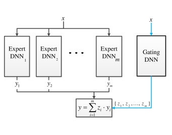
Figure 1: Deep Mixture of Experts (DMoE) architecture.

We next address the problem of learning the MoE parameters (i.e. the parameters of the experts and the gating function) given a training dataset $(x_{1},y_{1}),\dots,(x_{n},y_{n})$. The likelihood function of the MoE model parameters is:

$$L(\theta)=L(\theta_{g},\theta_{1},...,\theta_{m})=\sum_{t}\log p(y_{t}|x_{t};\theta).$$ (7)

Since the selected expert used to produce $y_{t}$ from the feature set $x_{t}$ (i.e. the value of the r.v. $z_{t}$) is hidden, it is natural to apply the EM algorithm to find the maximum-likelihood parameters [9]. The EM auxiliary function is:

$$Q(\theta,\theta^{0})=E_{p(z|x,y;\theta^{0})}(\log p(y,z|x;\theta))$$ (8)

such that $\theta^{0}$ is the current parameter estimation. In the E-step we apply Bayes’ rule to estimate the value of the selected expert based on the current parameter estimation:

$$w_{ti}=p(z_{t}=i|x_{t},y_{t};\theta^{0})=\frac{p(y_{t}|x_{t},z_{t}=i)p(z_{t}=i|x_{t})}{p(y_{t}|x_{t})}.$$ (9)

The M-step decouples the parameter estimation of the different components of the MoE model. We can optimize each of the experts and the gating function separately. The updated parameters of the gating function are obtained by maximizing the weighted likelihood function:

$$L(\theta_{g})=\sum_{t}\sum_{i}w_{ti}\log p(z_{t}=i|x_{t};\theta_{g})$$ (10)

and the updated parameters of the $i$-th expert are obtained by maximizing the function:

$$L(\theta_{i})=\sum_{t}w_{ti}\log p(y_{t}|x_{t},z_{t}=i;\theta_{i})$$ (11)

The general EM theory guarantees a monotone convergence of the model-parameter estimations (to a local maximum).

In the case where both the experts and the gating functions are implemented by DNNs, we denote this modal Deep Mixture of Experts (DMoE). The compound DNN model is expressed as follows:

$$p_{\mbox{\tiny NN}}(y|x;\theta)=\sum_{i}p_{\mbox{\tiny NN}}(z=i|x;\theta_{g})p_{\mbox{\tiny NN}}(y|z=i,x;\theta_{i}).$$ (12)

In this model $\theta_{g}$ is the parameter-set of the DNN that implements the gating function and $\theta_{i}$ is the parameter-set of the DNN that implements the $i$-th expert. We can still apply the EM algorithm described above to train the a DMoE. In this case in the M-step we need to train the experts and gating neural networks using the cross-entropy cost function defined by Eq. (10) and (11). We can thus iterate between EM steps and DNN training.

There are, however, several drawbacks to using the EM algorithm to train a DMoE. In each M-step iteration we need to train a new DNN. There is no closed-form solution for this non-concave maximization task. The DNN learning is performed by a stochastic gradient ascent and there is no guarantee for monotone improvement of the likelihood score. The EM algorithm is a greedy optimization procedure that is notorious for getting stuck in local optima. In most EM applications there is a closed-form solution for the optimization performed at the M-step. Here, since we need to retrain the experts and gating DNNs at each M-step (10) (11), even a monotone improvement of the likelihood is not guaranteed. The main problem of iterating between EM-steps and neural network training, however, is that it does not scale well. The framework requires training a neural network in each iteration of the EM algorithm. For real-world, large-scale networks, even a single training iteration is a non-trivial challenge.

In this study we replace the EM algorithm, which learns the expert and gating networks at each step separately, by a neural-network training procedure that simultaneously trains all the sub-networks by directly maximizing the likelihood function

$$L(\theta)=\sum_{t=1}^{n}\log(\sum_{i=1}^{m}p_{\text{{\tiny NN}}}(z_{t}=i|x_{t};\theta_{g})\cdot p_{\text{{\tiny NN}}}(y_{t}|z_{t}=i,x_{t};\theta_{i}))$$ (13)

In this architecture, the experts and the gating networks are components of a single network and are simultaneously trained with the same objective function. In order to update the network parameters we apply a back-propagation algorithm. It can be easily verified that the back propagation equation for the parameter set of the $i$-th expert is:

$$\frac{\partial L}{\partial\boldsymbol{\boldsymbol{\theta}}_{i}}=\sum_{t}w_{ti}\cdot\frac{\partial}{\partial\boldsymbol{\theta}_{i}}\log p_{\text{{\tiny NN}}}(y_{t}|z_{t}=i,x_{t};\theta_{i})$$ (14)

such that $w_{ti}$ is the posterior distribution of the gating random variable:

$$w_{ti}= p_{\text{{\tiny NN}}}(z_{t}=i|x_{t},y_{t};\theta)=$$ (15)

$$\frac{p_{\text{{\tiny NN}}}(y_{t}|x_{t},z_{t}=i;\theta_{i})p_{\text{{\tiny NN}}}(z_{t}=i|x_{t};\theta_{g})}{p_{\text{{\tiny NN}}}(y_{t}|x_{t};\theta)}.$$

Note that this definition coincides with the E-step of the EM algorithm defined in Eq. (9). In a similar way, the back-propagation equation for the parameter set of the gating DNN is:

$$\frac{\partial L}{\partial\boldsymbol{\boldsymbol{\theta}}_{g}}=\sum_{t}\sum_{i}w_{ti}\cdot\frac{\partial}{\partial\boldsymbol{\theta}_{g}}\log p_{\text{{\tiny NN}}}(z_{t}=i|x_{t};\theta_{g}).$$ (16)

Note, that the back-propagation partial derivatives (14) and (16) are exactly the derivatives of the functions (10) and (11) that are optimized by the M-step of the EM algorithm. By training all the components of the DMoE simultaneously we thus replace the two steps of the EM iterations by the single step of a gradient ascent optimization.

IV Deep Mixture Experts for Speech Enhancement

In this section we apply the DMoE principle to a speech enhancement task and describe the network specifics and training procedure.

IV-A Network description

The goal in a speech enhancement task is to find an accurate SPP, $\boldsymbol{\rho}$ from a given noisy signal $\mathbf{x}$ using the DMoE model. All the $m$ experts in the proposed algorithm are implemented by DNNs with the same structure. The input to each DNN is the noisy log-spectrum frame together with context frames. The network consists of 3 fully connected hidden layers with 500 rectified linear unit (ReLU) neurons each.

The output layer that provides the SPP binary decisions is composed of $L/2$ sigmoid neurons, one for each frequency band. The SPP decision of the $i$-th expert on the $k$-th frequency bin is:

$$\rho_{i,k}=p(b_{k}=1|\mathbf{x};\theta_{i}).$$ (17)

Let $h_{i}(\mathbf{x})$ be the value of the final hidden layer of the $i$-th expert. The SPP prediction can be written as $\rho_{i,k}=\sigma(w_{ik}h_{i}(\mathbf{x})+a_{ik})$ such that $\sigma$ is the sigmoid transfer function and $w_{ik},a_{ik}$ are the parameters of the affine input function to the sigmoid neuron. The fact that all the frequency bands are simultaneously estimated from $h_{i}(\mathbf{x})$ enables the network to reconstruct the harmonic structure.

Although the standard MoE approach uses the same input features for both the experts and the gating networks, here the log-spectrum of the noisy signal, $\mathbf{x}$, is utilized as the input for the experts alone, and the gating DNN is fed with the corresponding mel-frequency cepstral coefficients (MFCC) features denoted by $\mathbf{v}$. MFCC, which is based on frequency bands, is a more compact representation than a linearly spaced log-spectrum and this frequency warping is known for its better representation of sound classes [21]. We found that using the MFCC representation for the gating DNN both slightly improves performance and significantly reduces the input size.

The architecture of the gating DNN is also composed of 3 fully connected hidden layers with 500 ReLU neurons each. The output layer here is a softmax function that produces the gating distribution on the $m$ experts. The gating procedure therefore is:

$$p_{i}=p(z=i|\mathbf{v};\theta_{g}).$$ (18)

The final SPP is obtained by a weighted average of the deep experts’ decisions:

$$\boldsymbol{\rho}=\sum_{i=1}^{m}p_{i}\cdot\boldsymbol{\rho}_{i}.$$ (19)

Given the SPP vector $\boldsymbol{\rho}$, the enhanced signal is finally obtained using Eq. (5). The suggested DMoE algorithm for speech enhancement is presented in Algorithm 1.

The network was implemented in Keras [22] on top of Theano backend [23] with ADAM optimizer [24]. To overcome the mismatch between the training and the test conditions, each utterance was normalized prior to the training of the network, such that the sample-mean and sample-variance of the utterance were zero and one, respectively [25]. In order to circumvent over-fitting of the DNNs to the training database, we first applied the cepstral mean and variance normalization (CMVN) procedure to the input, prior to the training and test phases [25]. Additionally, the dropout method [26] was utilized on each layer. Finally, the batch-normalization method was applied to train acceleration on each layer [27].

IV-B Training the DMoE for speech enhancement

To train the network we need to collect a dataset of noisy speech and the corresponding binary vectors. Unlike [7], here neither a phoneme-labeled database nor pre-training are needed. Clean speech signals were contaminated with a single noise type in a pre-defined signal to noise ratio (SNR). The log-spectrum of the speech and the noise are known and a binary mask based on the maximization approximation (2) was then computed. Additionally, the corresponding MFCC features were calculated. Finally, in order to enhance the current frame of the noisy signal, context frame information is known to provide better performance; therefore, each input contained four context frames from the past and four from the future.

Assume the training set is $(\mathbf{x}_{1},\boldsymbol{b}_{1}),...(\mathbf{x}_{N},\boldsymbol{b}_{N})$ such that $\mathbf{x}_{t}$ is a log-spectrum of noisy speech and $\boldsymbol{b}_{t}$ is the corresponding binary mask vector, and $N$ is the length of the database. The training procedure aims to optimize the following log-likelihood function:.

$$L(\boldsymbol{\theta})=\sum_{t=1}^{N}\log p(\boldsymbol{b}_{t}|\mathbf{x}_{t};\theta)$$ (20)

such that

$$p(\boldsymbol{b}_{t}|\mathbf{x}_{t};\theta)=\sum_{i=1}^{m}p(z_{t}\!=\!i|\mathbf{v}_{t};\theta_{g})\prod_{k}p(b_{t}(k)|\mathbf{x}_{t},z_{t}\!=\!i;\theta_{i})$$ (21)

with $\mathbf{v}_{t}$, the MFCC coefficients at time $t$.

Input : 

• Noisy speech log-spectral vector $\mathbf{x}$.

• Corresponding MFCC feature vector $\mathbf{v}$.

• DMoE model parameters $\boldsymbol{\theta}=\{\boldsymbol{\theta}_{1},\ldots,\boldsymbol{\theta}_{m},\boldsymbol{\theta}_{g}\}$.

Output : Estimated log-spectral vector of the clean speech $\hat{\mathbf{s}}$.

Experts’ DNNs:

• Compute SPP decision for each expert $i\in\{1,\dots,m\}$ and for each frequency band $k$ (17):

  $$\rho_{i,k}=p(b_{k}=1|\mathbf{x};\theta_{i})$$

Gating DNN:

• Compute the gating distribution (18):

  $$p_{i}=p(z=i|\mathbf{v};\theta_{g})$$

Avergung Experts’ decsions:

• Compute final SPP (19)

  $$\boldsymbol{\rho}=\sum_{i=1}^{m}p_{i}\cdot\boldsymbol{\rho}_{i}$$

Enhancement:

• Estimate the clean speech (5):

  $$\hat{\mathbf{s}}=\boldsymbol{\rho}\cdot\mathbf{x}+(1-\boldsymbol{\rho})\cdot(\mathbf{x}-\beta).$$

Algorithm 1 DMoE speech enhancement algorithm.

Input : 

• Noisy speech log-spectral vectors $\mathbf{x}_{1},...,\mathbf{x}_{N}$

• Corresponding MFCC feature vectors $\mathbf{v}_{1},...,\mathbf{v}_{N}$

• Binary mask vectors $\boldsymbol{b}_{1},...,\boldsymbol{b}_{N}$

Output : DMoE model parameters $\boldsymbol{\theta}=\{\boldsymbol{\theta}_{1},\ldots,\boldsymbol{\theta}_{m},\boldsymbol{\theta}_{g}\}$.

Neural network training

Train a DNN in order to maximize the objective function:

$$L(\boldsymbol{\theta})=\sum_{t=1}^{n}\log(\sum_{i=1}^{m}p(z_{t}\!=\!i|\mathbf{v}_{t};\theta_{g})\prod_{k}p(b_{t}(k)|\mathbf{x}_{t},z_{t}\!=\!i;\theta_{i}))$$

Algorithm 2 DMoE training procedure.

The back-propagation partial derivative of the parameters of the $i$-th expert is:

$$\frac{\partial L}{\partial\boldsymbol{\boldsymbol{\theta}}_{i}}=\sum_{t}w_{ti}\cdot\frac{\partial}{\partial\boldsymbol{\theta}_{i}}\sum_{k}\log p(b_{t}(k)|z_{t}=i,x_{t};\theta_{i})$$ (22)

where $w_{ti}$ (see Eq. (9)) is the posterior probability that the $i$-th expert was used to produce the binary mask $\boldsymbol{b}_{t}$. The partial derivative of the gating parameter appears in (16).

Another decision we need to make is choosing the number of experts. We found that moving from a single expert to two experts yielded a significant improvement, but adding more experts had little effect. Hence, utilizing Occam’s razor principle, we chose the simpler model and set $m=2$. In Sec VI-A we show performance empirically as a function of the number of experts. We also show that when we train DMoE with two experts, the gating network tends to direct voiced frames to one expert and unvoiced frames to the second expert. The training procedure is summarized in Algorithm 2.

Train phase
	Database	Details
Supervised DMoE model	TIMIT (train set)	speech-like noise, SNR=10 dB, phoneme labels
DMoE	TIMIT (train set)	speech-like noise, SNR=10 dB
Test phase
	Database	Details
Speech	TIMIT (test set), WSJ
Noise	NOISEX-92	White, Speech-like, Room, Car, Babble, Factory
SNR	-	-5, 0, 5, 10, 15 dB
Objective measurements	-	PESQ, Composite measure

TABLE I: Experimental setup.

V Experimental study

In this section we present a comparative experimental study. We first describe the experiment setup in Sec. V-A. Objective quality measure results are then presented in Sec. V-B. Finally, the algorithm is tested on an untrained database in Sec. V-C.

V-A Experiment setup

To test the proposed DMoE algorithm we contaminated the speech signals with several types of noise from the NOISEX-92 database [28], namely Speech-like, Babble, Car, Room, AWGN and Factory. The noise was added to the clean signal drawn from the test set of the TIMIT database (24-speaker core test set), with 5 levels of SNR at $-5$ dB, $0$ dB, $5$ dB, $10$ dB and $15$ dB chosen to represent various real-life scenarios. The algorithm was also tested on the Wall Street Journal (WSJ) database [29] which was collected with a different recording setup. We compared the proposed algorithm to the OMLSA algorithm [2] with the IMCRA noise estimator [3] which is a state-of-the-art algorithm for single microphone speech enhancement. The default parameters of the OMLSA were set according to [30]. Additionally, we compared the proposed DMoE algorithm to two other DNN-based algorithms. The first DNN has a fully-connected architecture and can be viewed as a single-expert network. We denote this network the Deep Single Expert (DSE). The second DNN is a supervised phoneme-based DMoE architecture [7]. The network has 39 experts where each expert is explicitly associated with a specific phoneme and training uses the phoneme labeling available in the TIMIT dataset. We denoted this phoneme-based supervised network by S-DMoE. Each expert component in the DSE and S-DMoE networks has the same network architecture as the expert components of the proposed DMoE model.

Training Procedure

In order to carry out a fair comparison, all the DNN-based algorithms were trained with the same database. We used the TIMIT database [31] train set for the training phase and the test set for the testing. Note, that the train and test sets of TIMIT do not overlap. Clean utterances were contaminated with Speech-like noise with an SNR $=10$ dB. Note, that unlike most DNN-based algorithms [5], we trained the DMoE network only on a single noise type with a single pre-defined SNR value. The speech diversity modeling provided by the expert-set was found to be rich enough to handle noise types that were not presented in the training phase.

In order to evaluate the performance of the proposed speech enhancement algorithm, several objective and subjective measures were used. The standard perceptual evaluation of speech quality (PESQ) measure, which is known to have a high correlation with subjective score [32], was used. Additionally, the composite measure suggested by Hu and Loizou [33], was implemented. The composite measure weights the log likelihood ratio (LLR), the PESQ and the weighted spectral slope (WSS) [34] to predict the rating of the background distortion (Cbak), the speech distortion (Csig) and the overall quality (Covl) performance. The rating was based on the 1-5 mean opinion score (MOS) scale, and the clean speech signal had a MOS value of 4.5.

Finally, we also carried out informal listening tests with approximately thirty listeners. Table I summarizes the experimental setup.

V-B Objective quality measure results

We first evaluated the objective results of the proposed DMoE algorithm and compared it with the results obtained by the state-of-the-art OMLSA algorithm, the DSE and the S-DMoE phoneme-based algorithm [7]. The test set was the core test-set of the TIMIT database.

Fig. 2 depicts the PESQ results for all algorithms for the Speech-like, Room, Factory and Babble noise types as a function of the input SNR. In Fig. 4 we show the Covl results for the same noises.

It is evident that the proposed DMoE algorithm outperformed the competing algorithms on the two objective measures.

In order to gain further insights into the capabilities of the proposed algorithm we compared the enhancement performance of the DMoE algorithm with the challenging Factory noise environment. We set the SNR in this experiment to $5$ dB. Fig. 3 depicts the SPP comparison between the DSE, the S-DMoE and the proposed DMoE algorithm performance. Clearly the DSE is very noisy, and the DMoE is smoother than the S-DMoE in both the time and frequency domains.

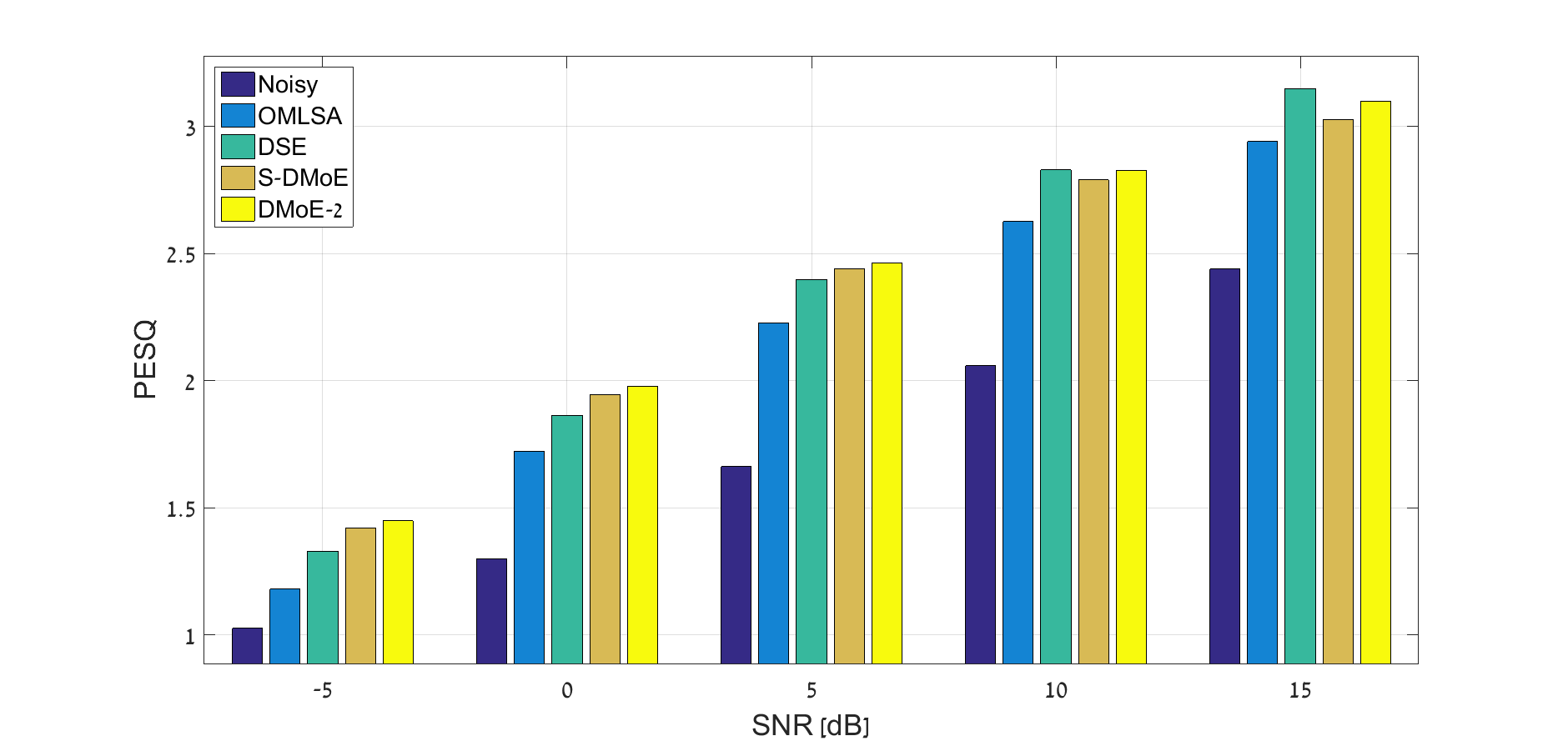
(a) Speech noise.

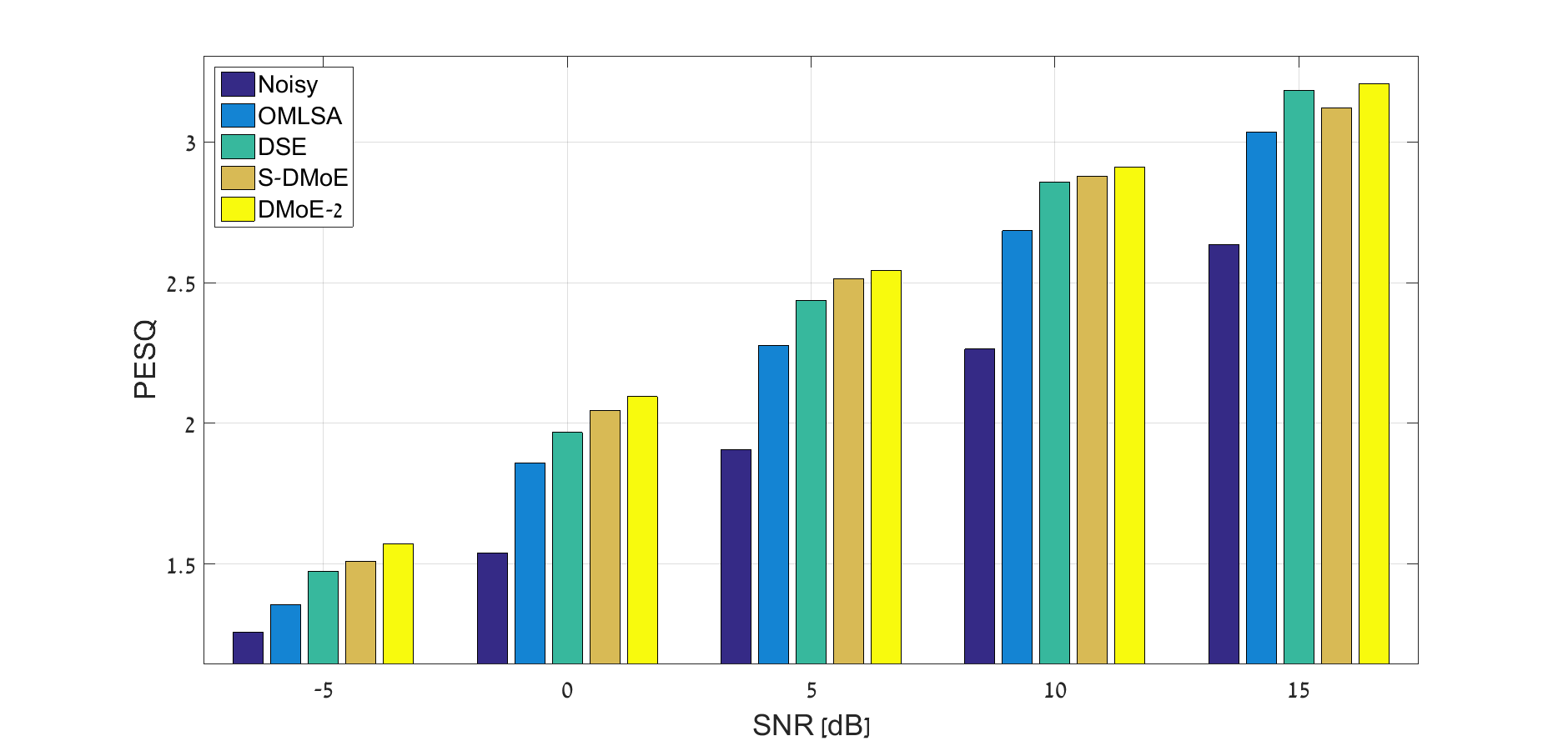
(b) Room noise.

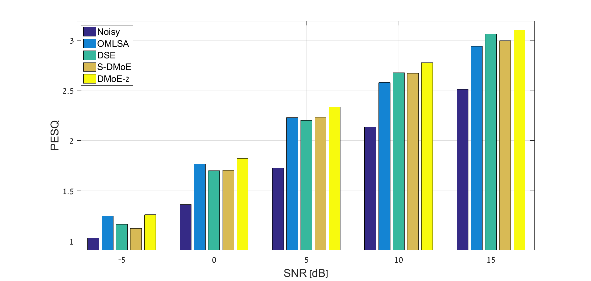
(c) Factory noise.

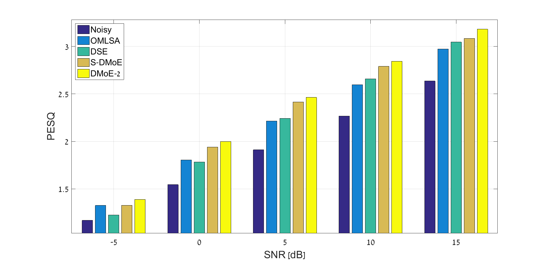
(d) Babble noise.

Figure 2: Speech quality results (PESQ) on the TIMIT test-set for several noise types.

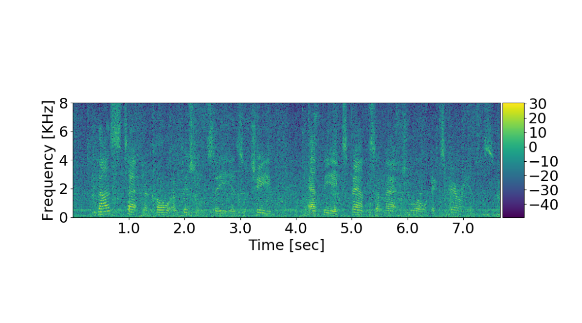
(a) Noisy.

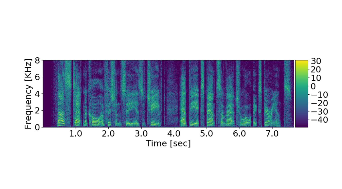
(b) Clean.

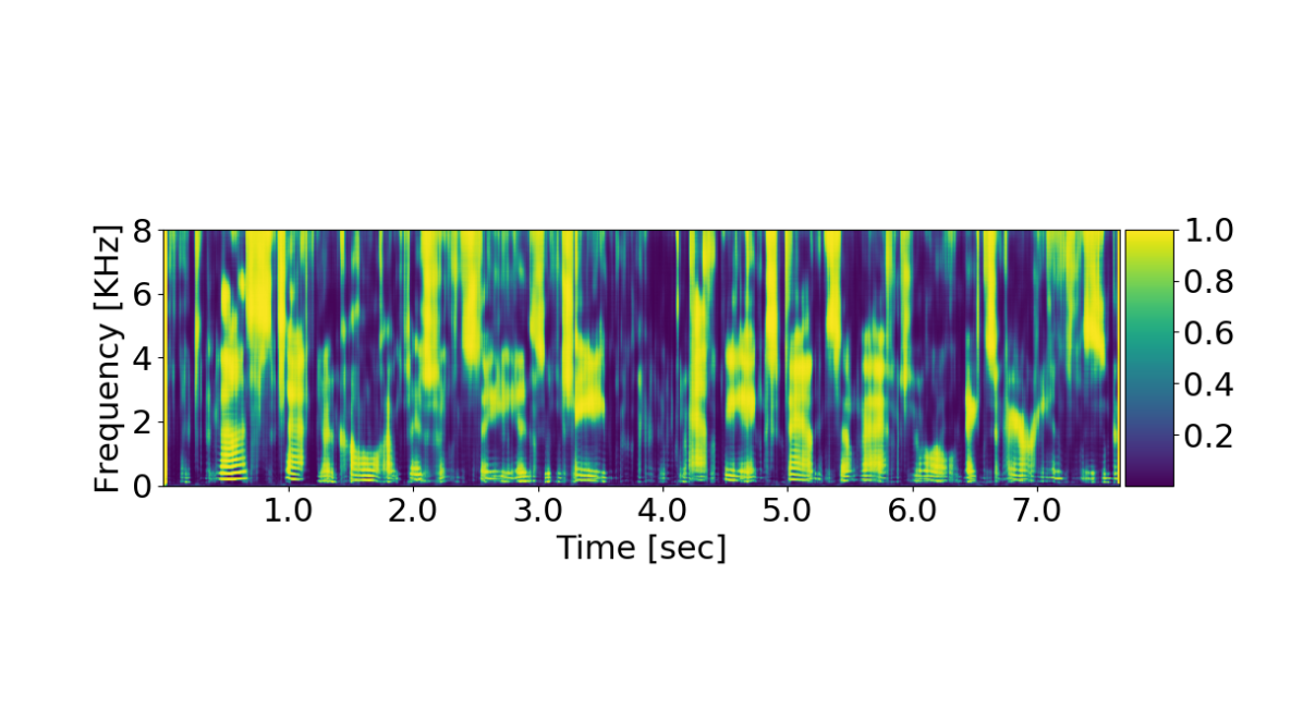
(c) DSE SPP.

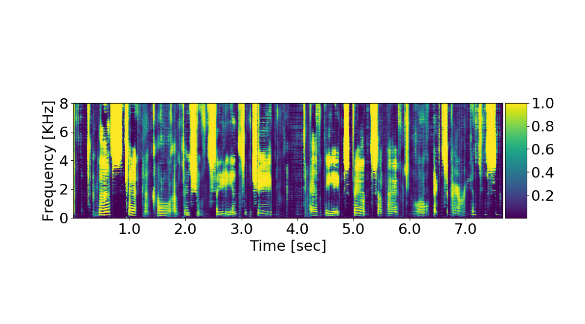
(d) S-DMoE SPP.

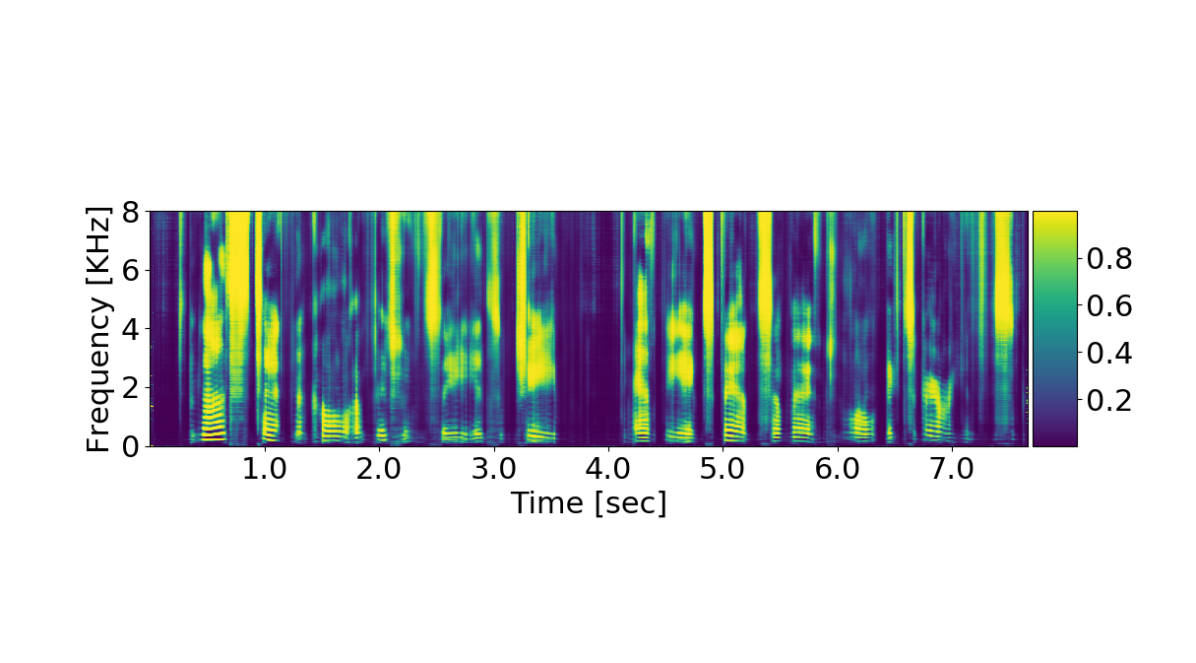
(e) DMoE-2 SPP.

Figure 3: SPP estimations of Factory noise with SNR = 5dB.

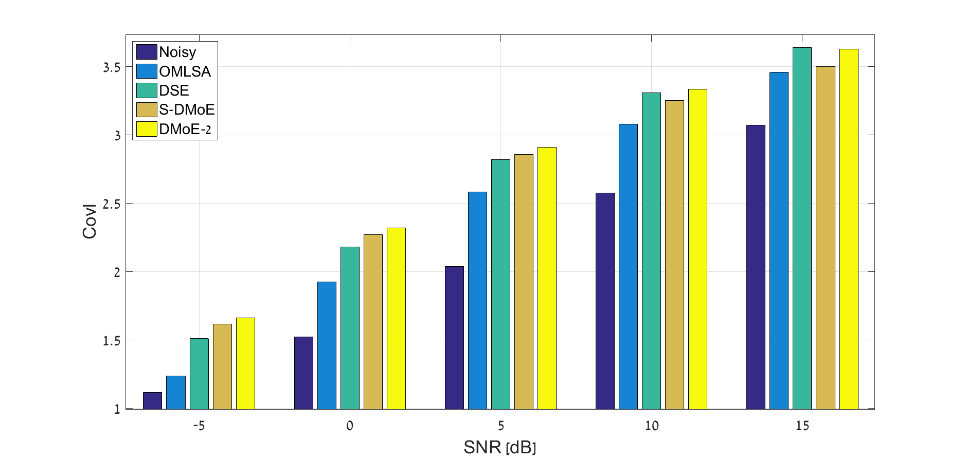
(a) Speech noise.

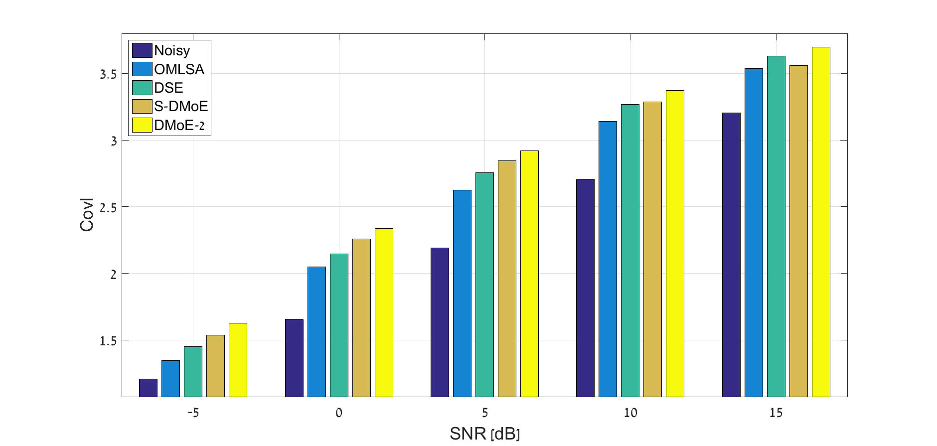
(b) Room noise.

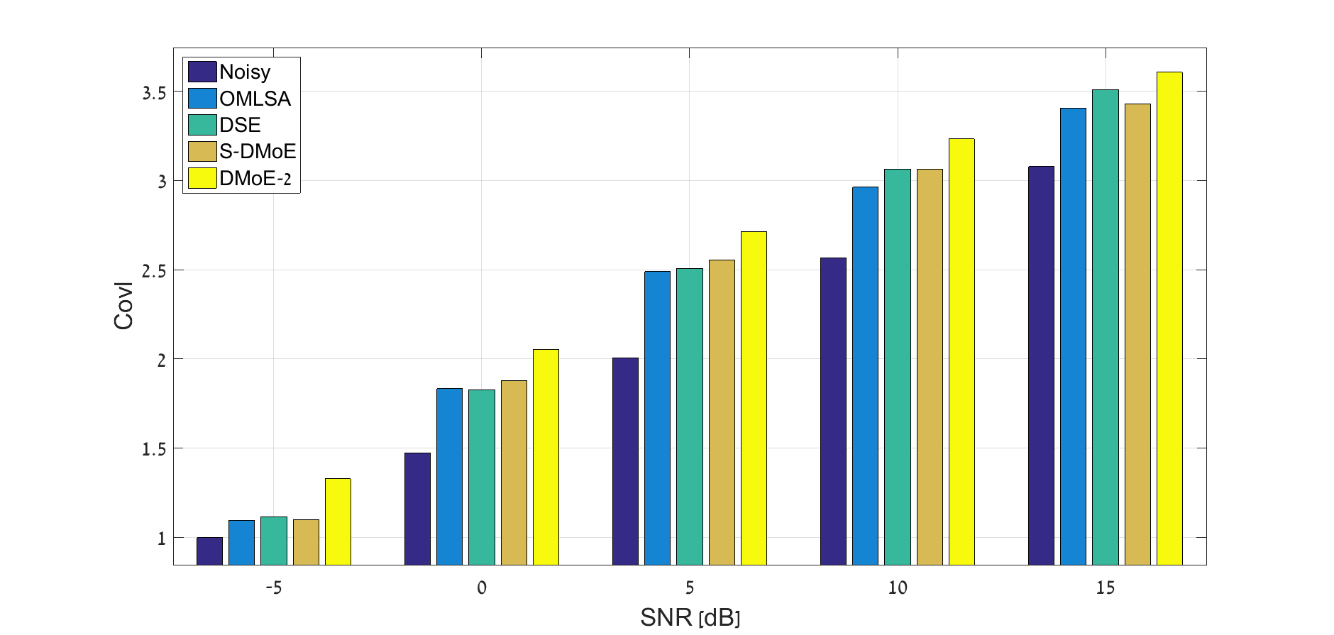
(c) Factory noise.

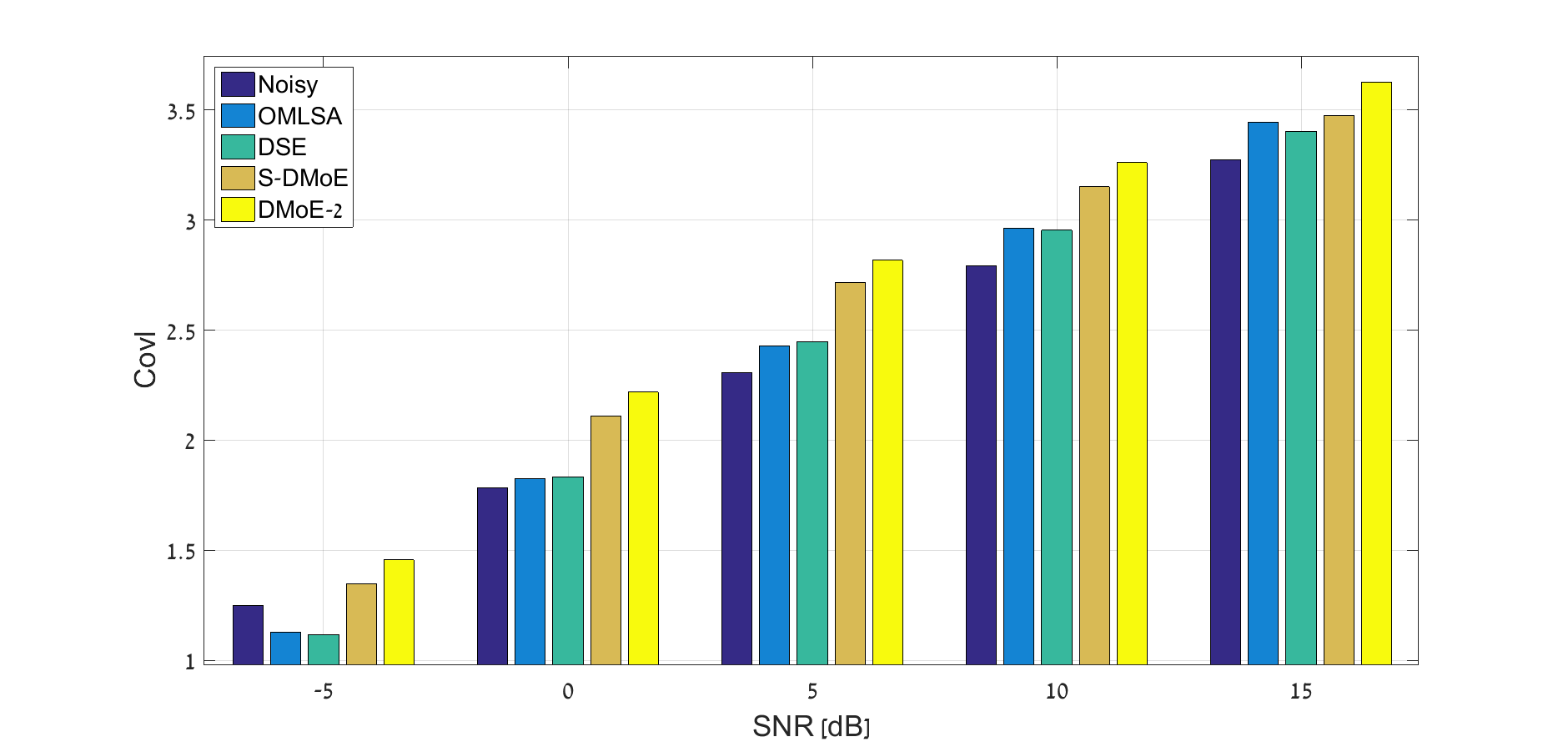
(d) Babble noise.

Figure 4: Speech quality results (Covl) on the TIMIT test-set for several noise types.

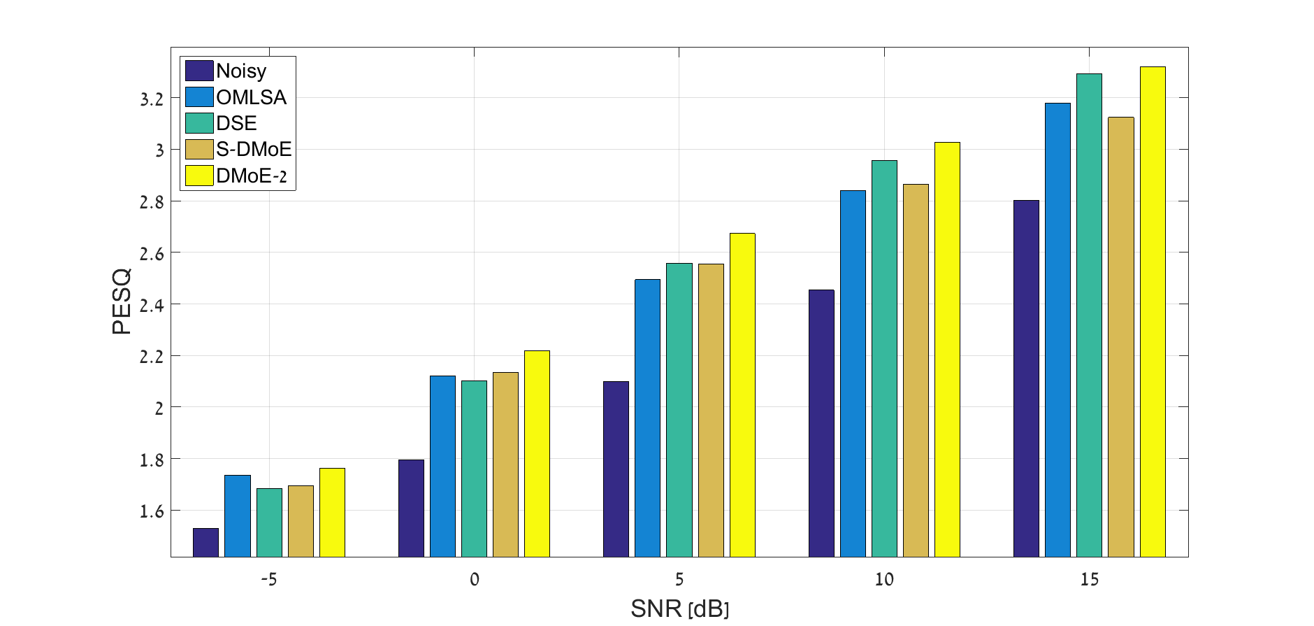
(a) Speech noise.

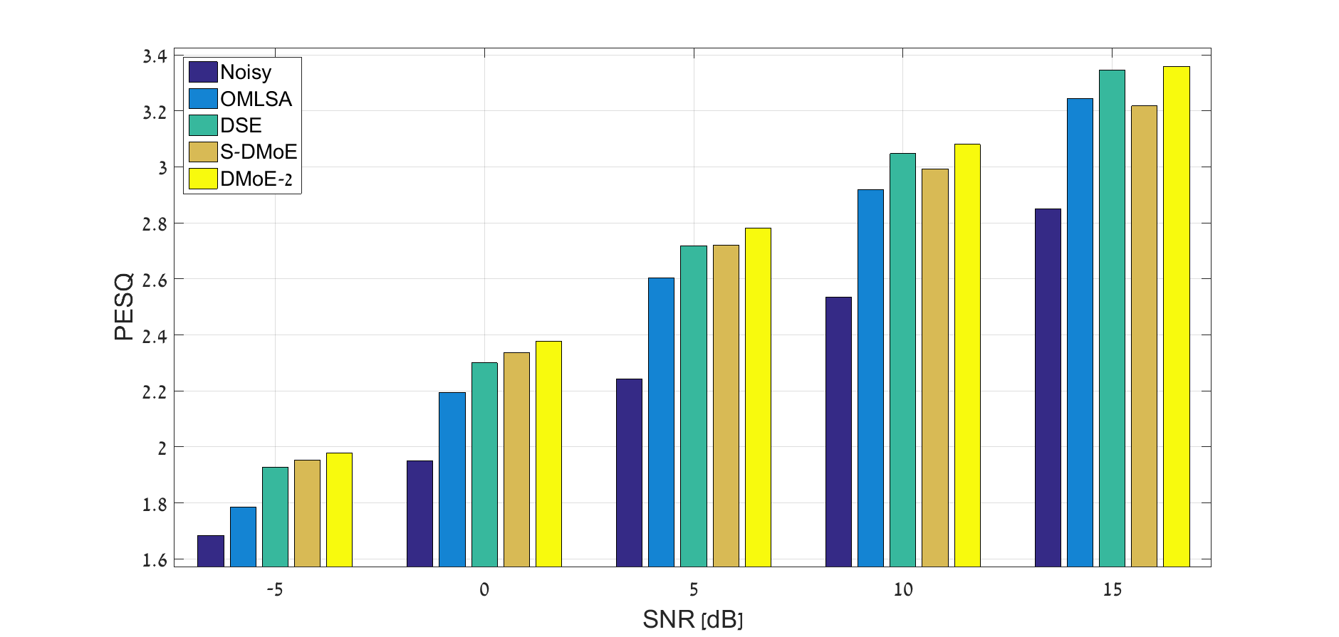
(b) Room noise.

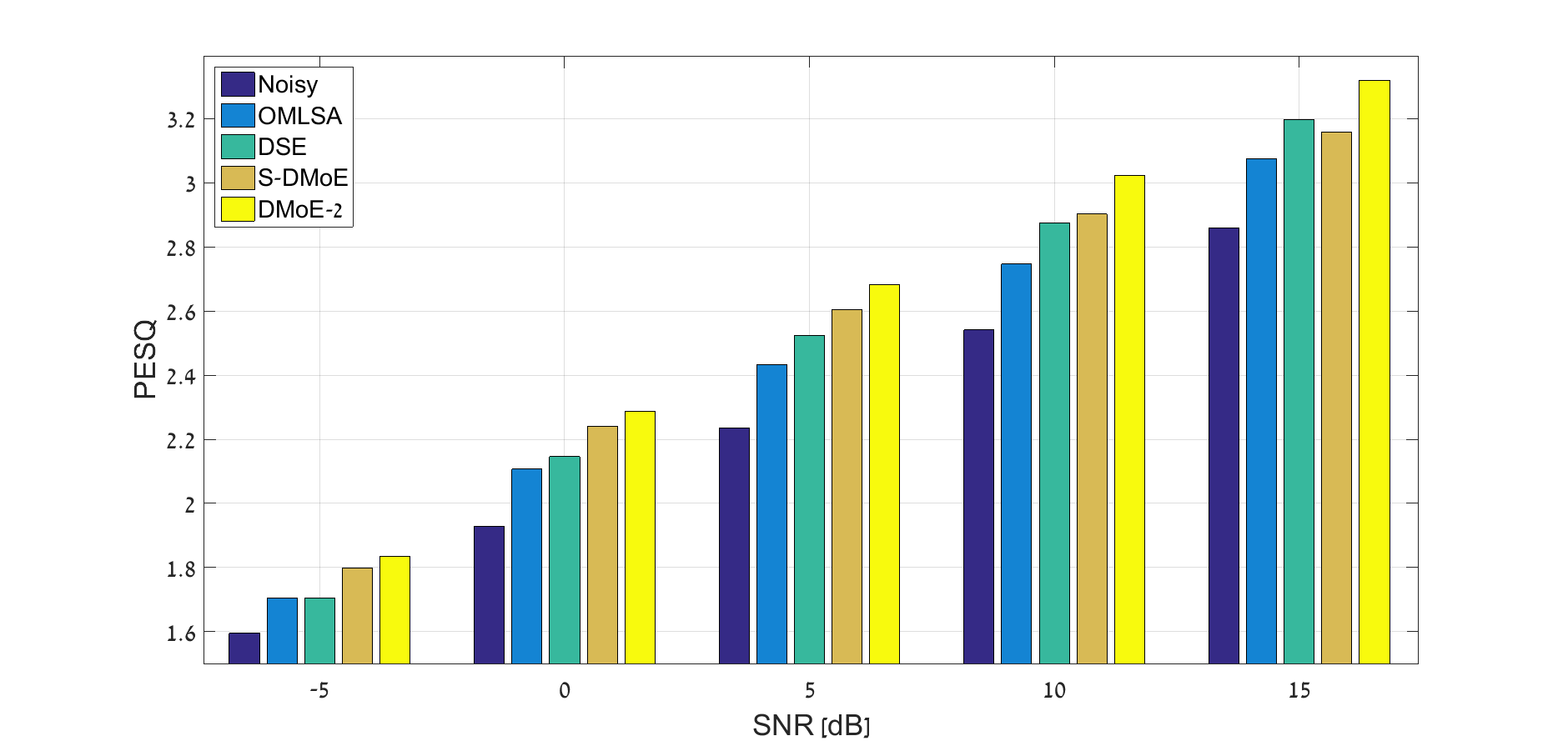
(c) Factory noise.

Figure 5: Speech quality results (PESQ) computed on the WSJ database.

V-C Performance with a different database

Here we have trained the DMoE using the TIMIT database. In order to show that the proposed algorithm is immune from the overfitting phenomena we tested the capabilities of the proposed DMoE algorithm when applied to speech signals from other databases. We applied the algorithm to $30$ clean signals drawn from the WSJ database [29]. The signals were contaminated by Speech, Room and Factory noises, drawn from the NOISEX-92 database, with several SNR levels. Note, that the algorithm was neither trained on that database nor trained with these noise types. Fig. 5 depicts the PESQ measure of the DMoE algorithm in comparison to the other algorithms. It is evident that the performance of proposed algorithm was maintained even for sentences drawn from a database other than the training database. The results for other noise types, not shown here due to space constraints, were comparable.

VI Discussion

In this section, we first discuss the role of the number of experts in Sec VI-A. The experts’ performance is tested in Sec VI-B, and finally, the gating is analyzed in Sec VI-C.

VI-A Setting the number of experts

The proposed architecture is based on a mixture of $m$ experts and the gating network directs a given input to one of these $m$ experts. In most MoE studies, finding the number of experts was done by exhaustive search [12]. In our case we divide the (log-spectrum) feature space into $m$ simpler subspaces. On one hand, setting a large value for $m$ divides the problem into many experts thus giving each expert an easier job of enhancing a distinct speech type. On the other hand, when $m$ is large the model complexity is higher, which makes the training task more difficult. Additionally, when the model size is large, the computational demands can make it difficult to use in real time applications. In order to determine the best value of $m$ based on enhancement performance, we conducted an experiment using DMoE models with 1, 2, 10, 20, 30 and 39 experts. We use the notation DMoE-$m$ for a DMoE based on $m$ experts. The 6 architectures were trained separately on the train part of the TIMIT database. We then tested the obtained networks using the same procedure described in Sec V-A. Fig. 6 shows the Covl results, and Fig. 7 shows the PESQ results. It is clear that moving from a single expert to two experts significantly improves the results. However, as can be seen from the results, further increasing the number of experts did not improve the performance much.

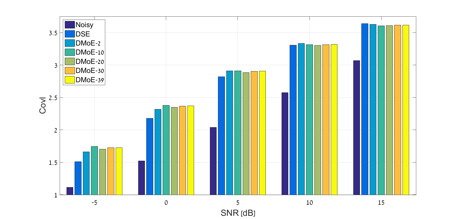
(a) Speech noise.

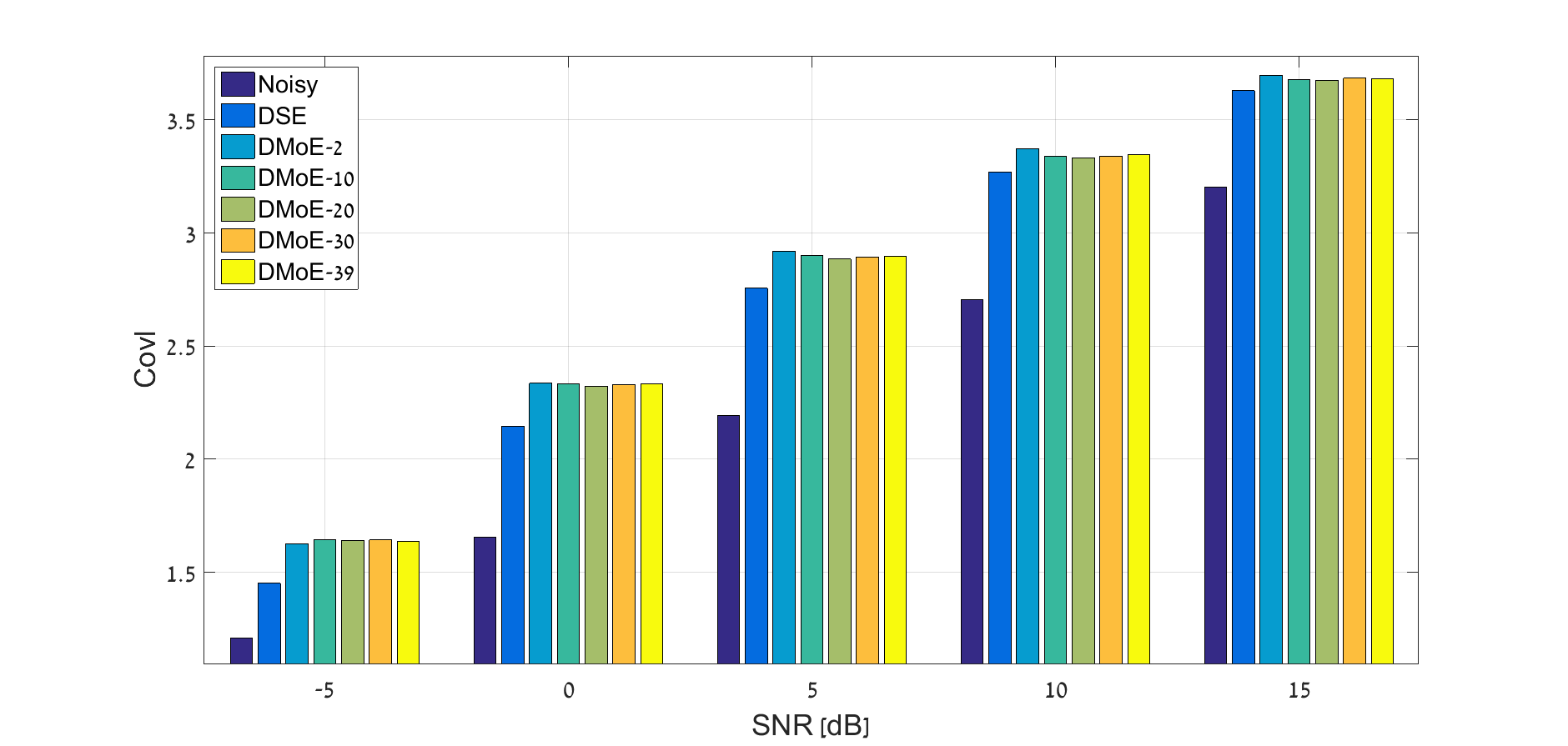
(b) Room noise.

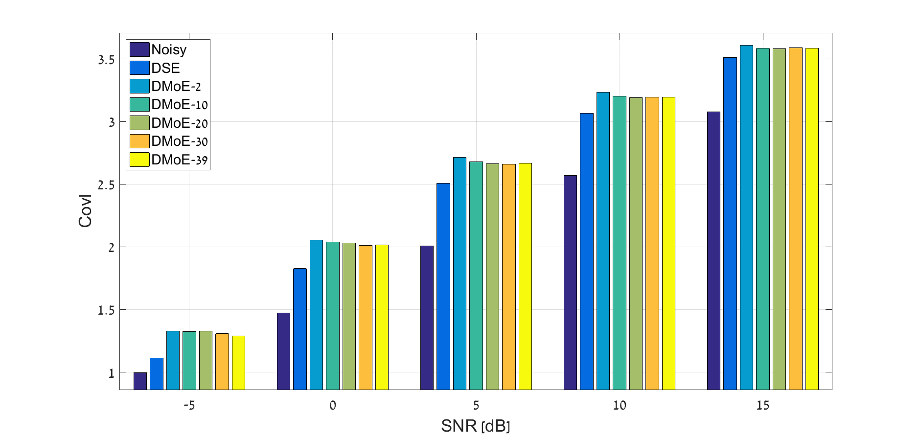
(c) Factory noise.

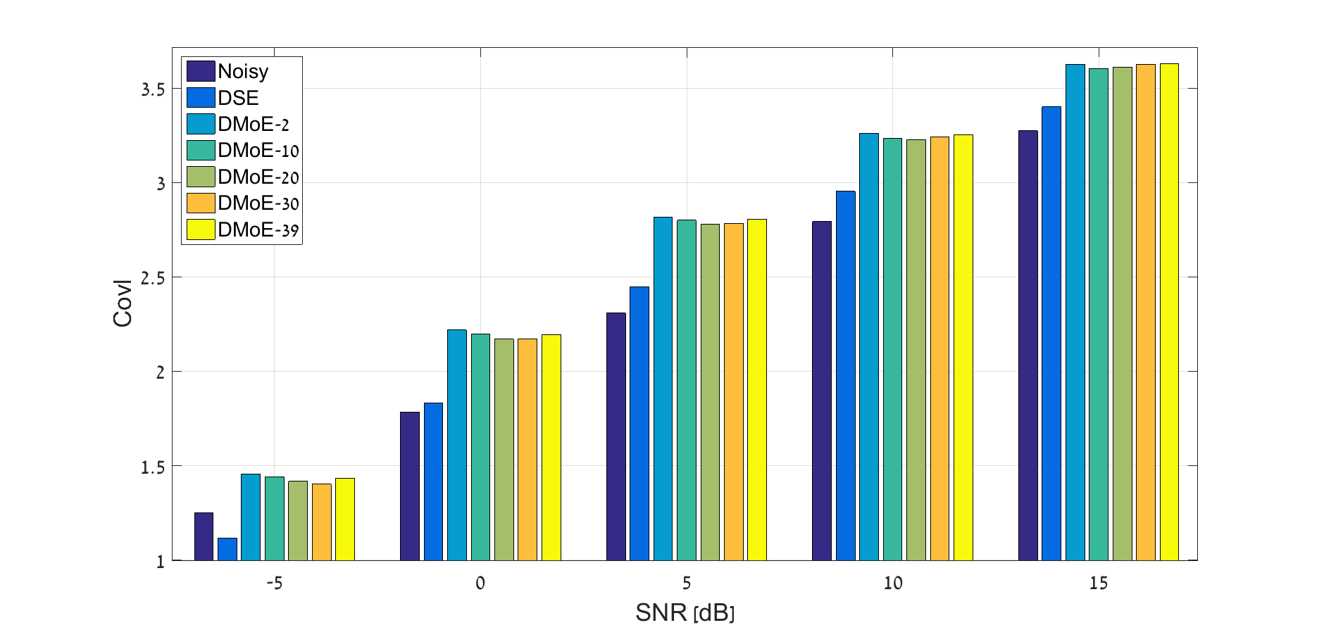
(d) Babble noise.

Figure 6: Speech quality results (Covl) for several noise types as a function of the number of experts.

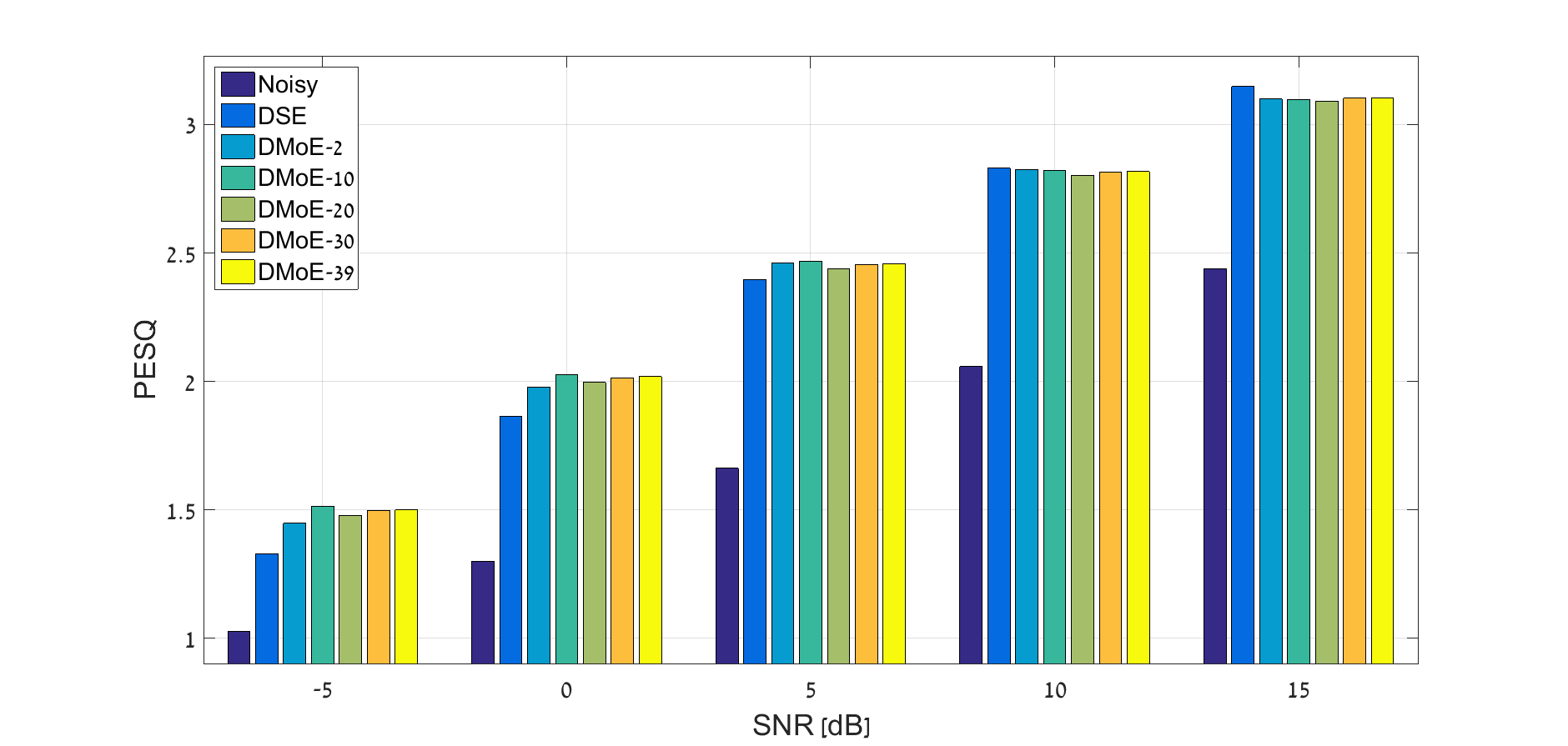
(a) Speech noise.

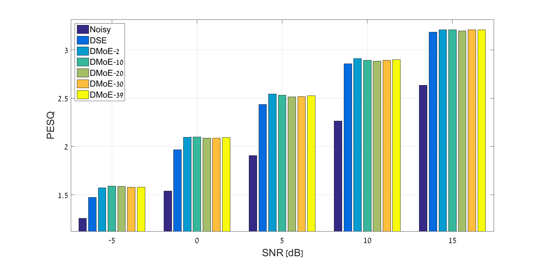
(b) Room noise.

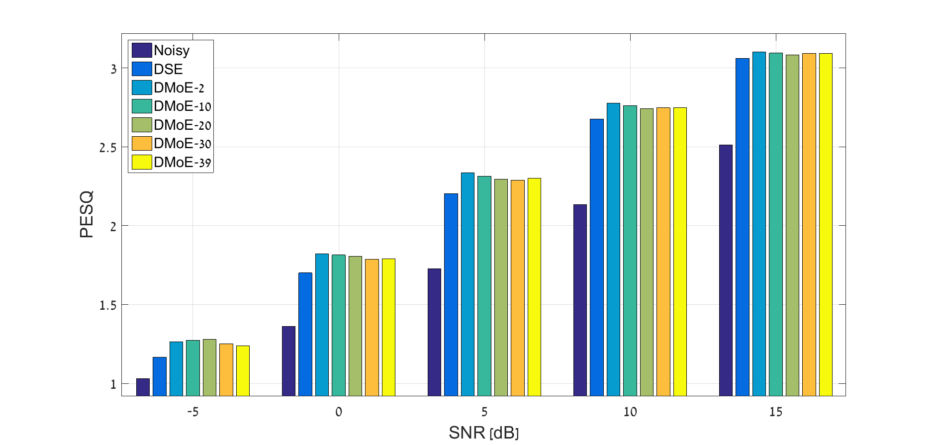
(c) Factory noise.

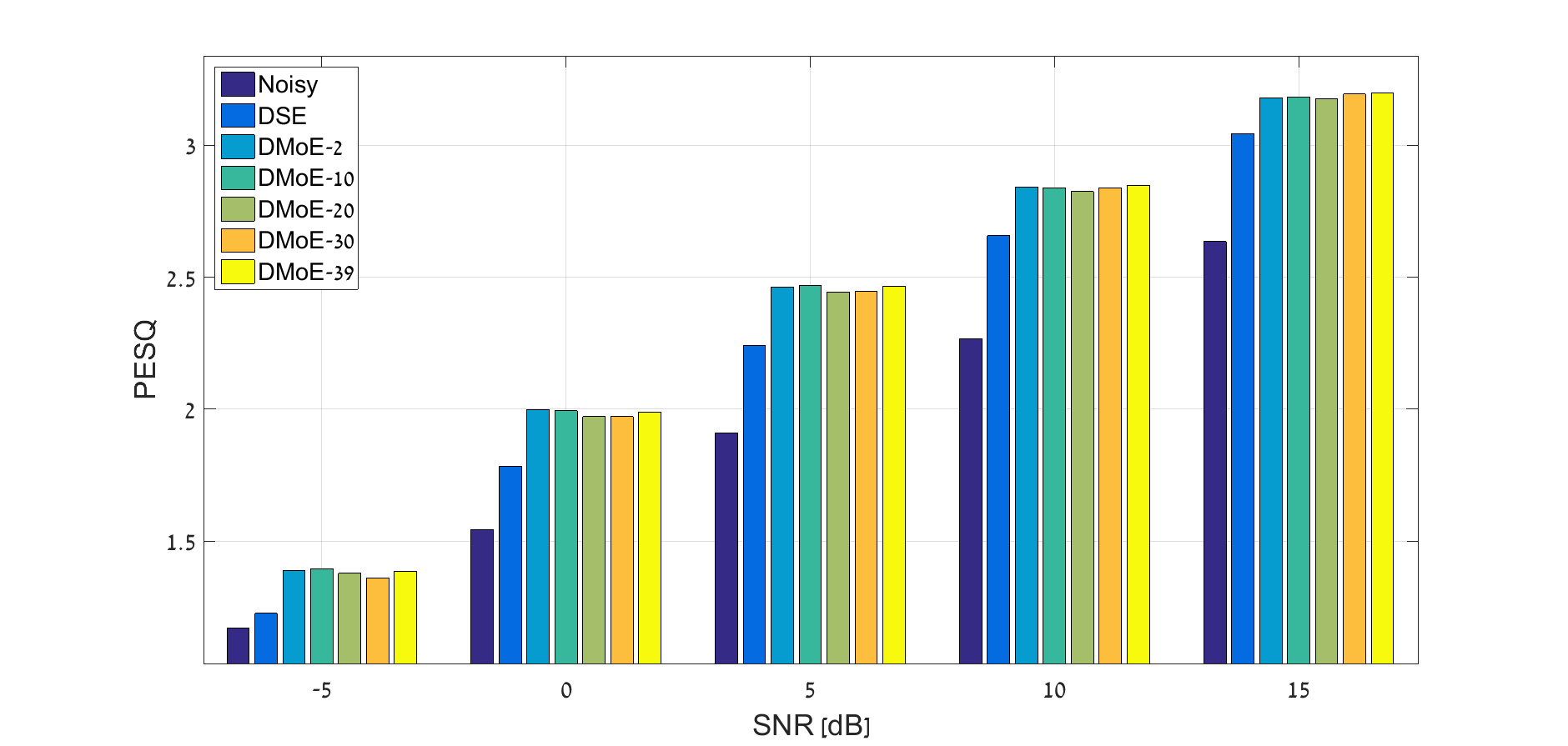
(d) Babble noise.

Figure 7: Speech quality results (PESQ) for several noise types as a function of the number of experts.

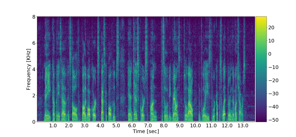
(a) Clean speech.

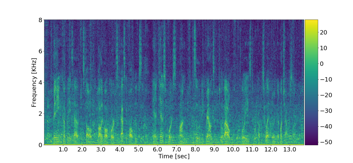
(b) Noisy speech.

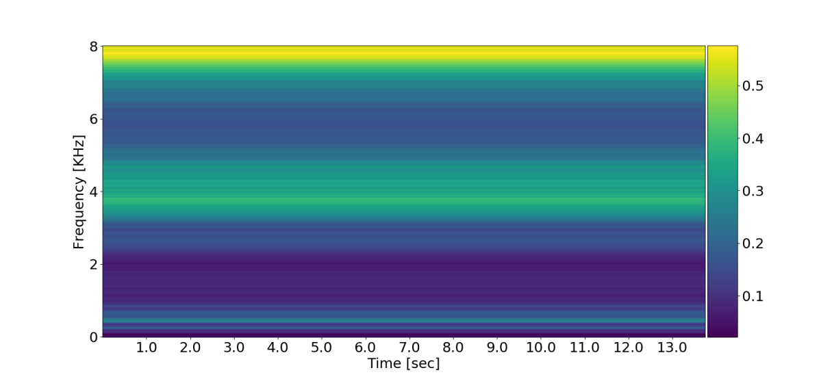
(c) DSE SPP.

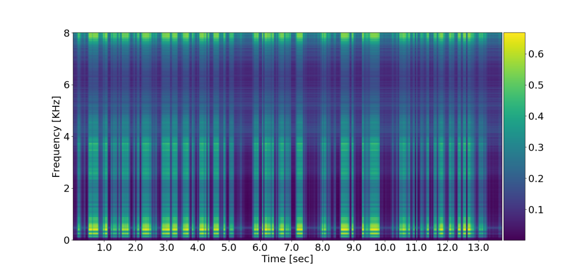
(d) DMoE-2 SPP.

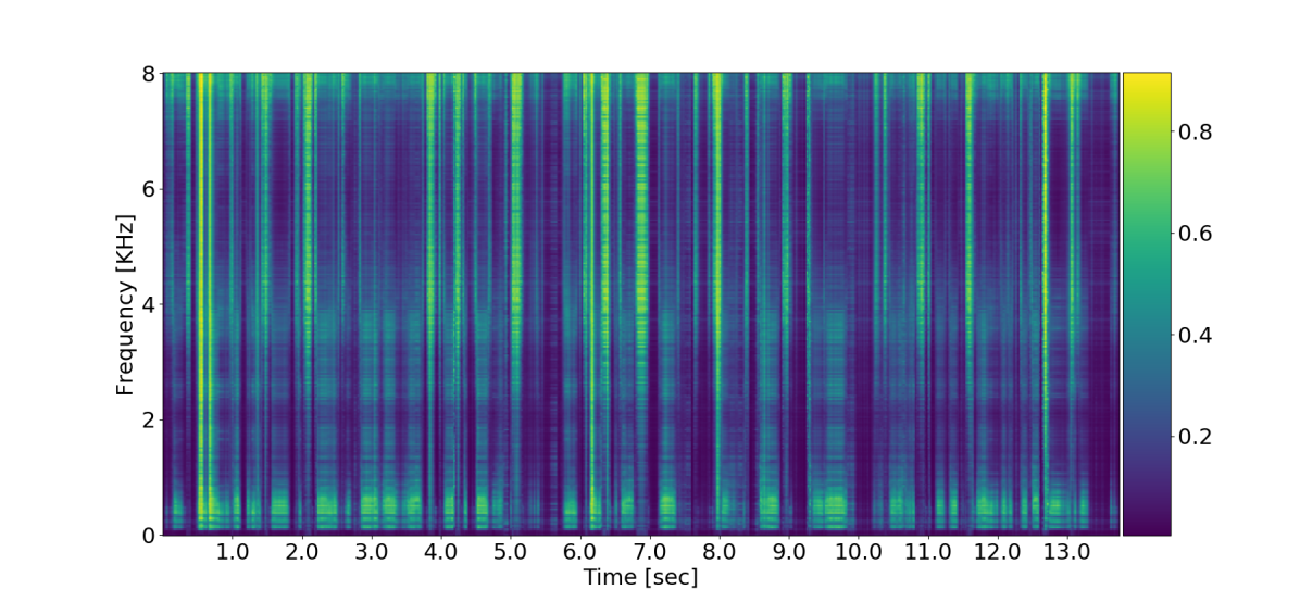
(e) DMoE-30 SPP.

Figure 8: Enhancement performance based solely on the input data to the gating network (and using a fixed non-informative vector as input to the experts’ networks). We show the estimated SPP for several speech enhancement networks.

VI-B The experts’ expertise

To illustrate the role of different experts, we added non-stationary Factory noise to clean speech from the TIMIT database with SNR=5 dB. The gating DNN was fed with the MFCC features of the noisy input and produced the probability of each expert. Now, instead of introducing the experts to the noisy log-spectrum vector $\mathbf{x}$, a vector of all-ones was used as input. This non-informative vector can be viewed as a noise-only signal. This vector propagated through the experts and in the end, the SPP $\boldsymbol{\rho}$ was estimated. Fig. 8 depicts the output of the enhancing procedure. Figs. 8(a) and 8(b) show the clean and noisy speech. Fig. 8(c) shows the estimated SPP of the fully-connected (single expert) architecture. It is clear that since the input is the same and the MFCC gating-decision data are irrelevant here, no information is preserved and the results therefore are meaningless. Fig. 8(d) shows the estimated SPP of the DMoE-2 architecture. Here, the extra information of the gating helps the experts to follow the structure of the input. Note, that only two different structures are shown here, based on the two experts. Simple inspection shows that one SPP structure appears in the voiced frames and the other in the unvoiced frames. Finally, in Fig. 8(e) the estimated SPP from DMoE-30 is depicted. It is easy to see that this architecture tracks the clean speech more accurately. Now that more experts are present, more speech structures are estimated.

This experiment suggests that each expert is responsible for a specific structure of the speech. Consequentially, the experts preserve the speech structure even if introduced to an unfamiliar noise. This leads to more robust behavior compared to other DNN-based algorithms.

VI-C The gating voice/unvoiced decision

Fig. 8(d) depicts the case of two experts, one responsible for enhancing voiced frames and the other for the unvoiced frames. The gating network therefore needs to classify the frame as voiced or unvoiced in order to direct it to the appropriate expert. We next show in a more systematic and quantitative manner that this is indeed what the gate network does. Note, that in the training phase no phoneme labels are provided to the gating DNN. The TIMIT database is phoneme labeled. Hence we can collect statistics on gate decisions for each phoneme separately. Fig. 9(a) depicts the gate decision statistic as a function of the phoneme label, and Fig. 9(b) presents the average structure of the phonemes in the log-spectrum domain. It appears from the gating decisions that the gating DNN tends to direct unvoiced phonemes to one expert and the voiced phonemes to the second. This partition, which is obtained in an unsupervised manner, makes sense since the voice/unvoiced structures are dramatically different: the voiced phonemes are characterized by energy in the low frequencies, whereas the unvoiced phonemes are characterized by energy in the high frequencies.

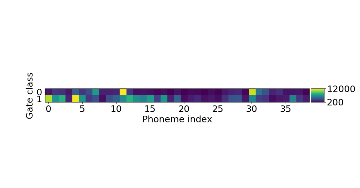
(a) The binary gating distribution for each phoneme.

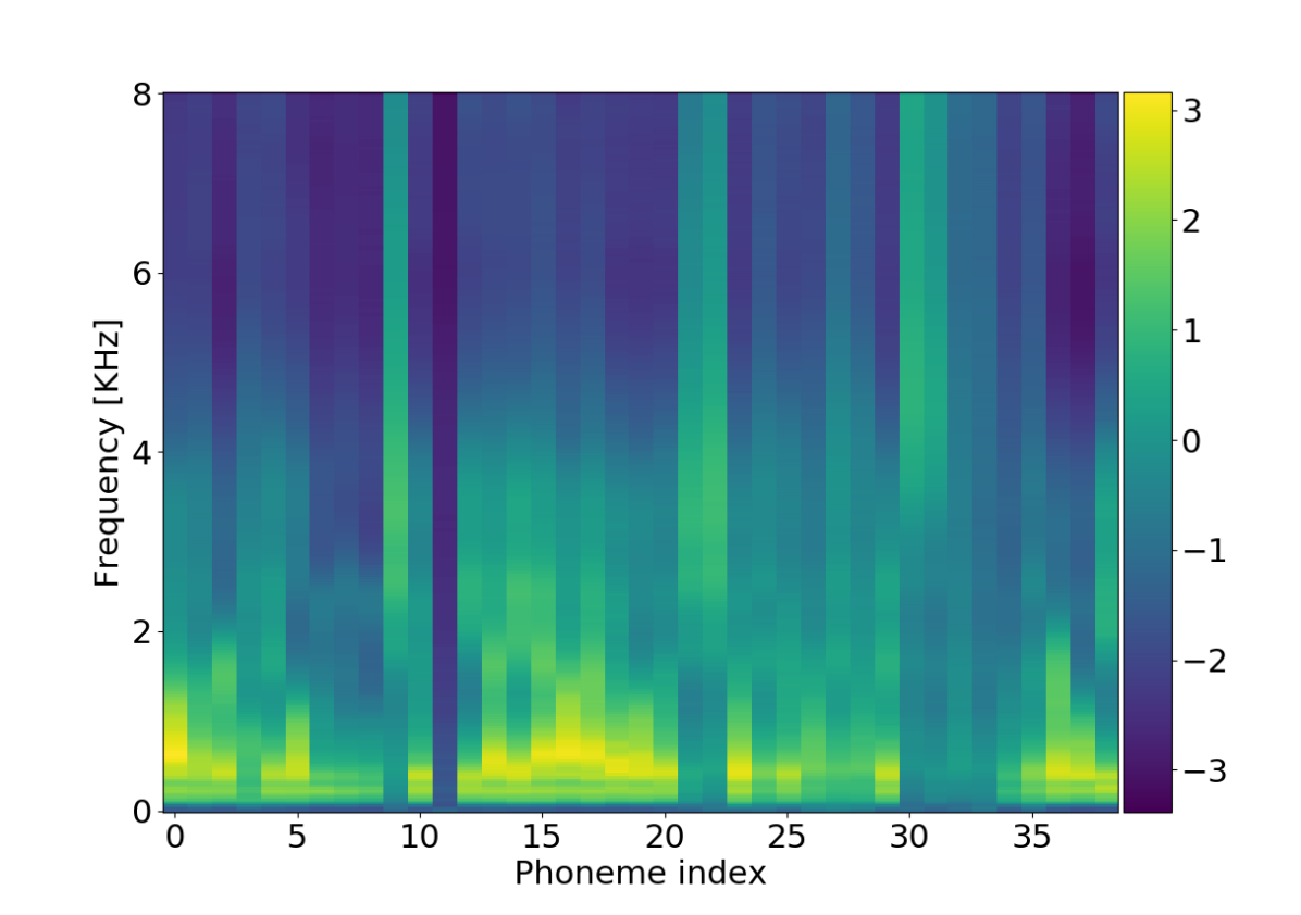
(b) Phonemes PSD.

Figure 9: Average phonemes distribution in the log-spectrum domain.

VII Conclusion

This article introduced a DMoE model for speech enhancement. This approach divides the challenging task of speech enhancement into simpler tasks where each DNN expert is responsible for a simpler one. The gating DNN directs the input features to the correct expert. We showed empirically that in the case of two experts, the gating decision is correlated with the voice/unvoiced status of the input frame.

In a fully connected DNN, the input to a single DNN has to deal with both voiced and unvoiced frames, which leads to performance degradation. On the other hand, in the DMoE model, the gating splits the problem into simpler problems and each expert preserves the pattern of the the spectral structure of frames that are directed to this expert. This approach makes is possible to overcome the well known problem of DNN-based algorithms; namely, the mismatch between training phase and test phase. Additionally, the proposed DMoE architecture enables training with a small database of noises.

The experiments showed that the proposed algorithm outperforms state of the art algorithms as well as DNN-based approaches on the basis of objective and subjective measurements.

References

- [1] P. C. Loizou, Speech enhancement: theory and practice. CRC press, 2013.
- [2] I. Cohen and B. Berdugo, “Speech enhancement for non-stationary noise environments,” Signal processing, vol. 81, no. 11, pp. 2403–2418, 2001.
- [3] ——, “Noise estimation by minima controlled recursive averaging for robust speech enhancement,” IEEE Signal Processing Letters, vol. 9, no. 1, pp. 12–15, Jan 2002.
- [4] X. Lu, Y. Tsao, S. Matsuda, and C. Hori, “Speech enhancement based on deep denoising autoencoder.” in INTERSPEECH, 2013, pp. 436–440.
- [5] Y. Wang, J. Chen, and D. Wang, “Deep neural network based supervised speech segregation generalizes to novel noises through large-scale training,” Dept. of Comput. Sci. and Eng., The Ohio State Univ., Columbus, OH, USA, Tech. Rep. OSU-CISRC-3/15-TR02, 2015.
- [6] Z.-Q. Wang, Y. Zhao, and D. Wang, “Phoneme-specific speech separation,” in IEEE International Conference on Acoustics, Speech and Signal Processing (ICASSP). IEEE, 2016, pp. 146–150.
- [7] S. E. Chazan, S. Gannot, and J. Goldberger, “A phoneme-based pre-training approach for deep neural network with application to speech enhancement,” in 2016 IEEE International Workshop on Acoustic Signal Enhancement (IWAENC), Sept 2016, pp. 1–5.
- [8] R. A. Jacobs, M. I. Jordan, S. J. Nowlan, and G. E. Hinton, “Adaptive mixtures of local experts,” Neural computation, vol. 3, no. 1, pp. 79–87, 1991.
- [9] M. I. Jordan and R. A. Jacobs, “Hierarchical mixtures of experts and the em algorithm,” Neural computation, vol. 6, no. 2, pp. 181–214, 1994.
- [10] R. Collobert, S. Bengio, and Y. Bengio, “A parallel mixture of svms for very large scale problems,” Neural computation, vol. 14, no. 5, pp. 1105–1114, 2002.
- [11] V. Tresp, “Mixtures of gaussian processes,” in NIPS, 2000, pp. 654–660.
- [12] S. E. Yuksel, J. N. Wilson, and P. D. Gader, “Twenty years of mixture of experts,” IEEE transactions on neural networks and learning systems, vol. 23, no. 8, pp. 1177–1193, 2012.
- [13] M. R. David Eigen and I. Sutskever, “Learning factored representations in a deep mixture of experts,” in ICLR Workshops, 2014.
- [14] A. Nádas, D. Nahamoo, and M. Picheny, “Speech recognition using noise-adaptive prototypes,” IEEE Trans. on Acoustics, Speech and Signal Processing, vol. 37, no. 10, pp. 1495–1503, Oct. 1989.
- [15] D. Burshtein and S. Gannot, “Speech enhancement using a mixture-maximum model,” IEEE Trans. on Speech and Audio Processing, vol. 10, no. 6, pp. 341–351, Sep. 2002.
- [16] Y. Yeminy, S. Gannot, and Y. Keller, “Speech enhancement using a multidimensional mixture-maximum model,” in International Workshop on Acoustic Echo and Noise Control (IWAENC), 2010.
- [17] S. E. Chazan, J. Goldberger, and S. Gannot, “A hybrid approach for speech enhancement using mog model and neural network phoneme classifier,” IEEE/ACM Transactions on Audio, Speech, and Language Processing, vol. 24, no. 12, pp. 2516–2530, Dec 2016.
- [18] S. T. Roweis, “One microphone source separation,” in Neural Information Processing Systems (NIPS), vol. 13, 2000, pp. 793–799.
- [19] M. Radfar and R. Dansereau, “Single-channel speech separation using soft mask filtering,” IEEE Trans. on Audio, Speech, and Language Processing, vol. 15, no. 8, pp. 2299–2310, Nov. 2007.
- [20] Y. Wang and D. Wang, “Towards scaling up classification-based speech separation,” IEEE Trans. on Audio, Speech, and Language Processing, vol. 21, no. 7, pp. 1381–1390, Jul. 2013.
- [21] H. Hermansky, J. R. Cohen, and R. M. Stern, “Perceptual properties of current speech recognition technology,” Proceedings of the IEEE, vol. 101, no. 9, pp. 1968–1985, Sept 2013.
- [22] F. Chollet, “Keras,” https://github.com/fchollet/keras, 2015.
- [23] R. Al-Rfou, G. Alain, A. Almahairi, C. Angermueller, D. Bahdanau, N. Ballas, F. Bastien, J. Bayer, A. Belikov, A. Belopolsky et al., “Theano: A python framework for fast computation of mathematical expressions,” arXiv preprint arXiv:1605.02688, 2016.
- [24] D. Kingma and J. Ba, “Adam: A method for stochastic optimization,” arXiv preprint arXiv:1412.6980, 2014.
- [25] J. Li, L. Deng, Y. Gong, and R. Haeb-Umbach, “An overview of noise-robust automatic speech recognition,” IEEE Trans. on Audio, Speech, and Language Processing, vol. 22, no. 4, pp. 745–777, Apr. 2014.
- [26] N. Srivastava, G. E. Hinton, A. Krizhevsky, I. Sutskever, and R. Salakhutdinov, “Dropout: a simple way to prevent neural networks from overfitting.” Journal of Machine Learning Research, vol. 15, no. 1, pp. 1929–1958, 2014.
- [27] S. Ioffe and C. Szegedy, “Batch normalization: Accelerating deep network training by reducing internal covariate shift,” arXiv preprint arXiv:1502.03167, 2015.
- [28] A. Varga and H. J. Steeneken, “Assessment for automatic speech recognition: Ii. NOISEX-92: A database and an experiment to study the effect of additive noise on speech recognition systems,” Speech communication, vol. 12, no. 3, pp. 247–251, 1993.
- [29] D. B. Paul and J. M. Baker, “The design for the wall street journal-based csr corpus,” in Proceedings of the Workshop on Speech and Natural Language, ser. HLT ’91. Stroudsburg, PA, USA: Association for Computational Linguistics, 1992, pp. 357–362.
- [30] “Matlab software for speech enhancement based on optimally modified lsa (OMLSA) speech estimator and improved minima controlled recursive averaging (IMCRA) noise estimation approach for robust speech enhancement,” http://webee.technion.ac.il/people/IsraelCohen/.
- [31] J. S. Garofalo, L. F. Lamel, W. M. Fisher, J. G. Fiscus, D. S. Pallett, and N. L. Dahlgren, “The DARPA TIMIT acoustic-phonetic continuous speech corpus CD-ROM,” Linguistic Data Consortium, Tech. Rep., 1993.
- [32] P. Recommendation, “862: Perceptual evaluation of speech quality (PESQ): An objective method for end-to-end speech quality assessment of narrow-band telephone networks and speech codecs,” Feb, vol. 14, pp. 14–0, 2001.
- [33] Y. Hu and P. Loizou, “Evaluation of objective quality measures for speech enhancement,” IEEE Trans. on Audio, Speech, and Language Processing, vol. 16, no. 1, pp. 229–238, Jan. 2008.
- [34] D. Klatt, “Prediction of perceived phonetic distance from critical-band spectra: A first step,” in IEEE International Conference on Acoustics, Speech and Signal Processing (ICASSP), vol. 7, May 1982, pp. 1278–1281.