Localization of fermions in coupled chains with identical disorder

Abstract

We study fermionic ladders with identical disorder along the leg direction. Following recent experiments we focus, in particular, on how an initial occupation imbalance evolves in time. By considering different initial states and different ladder geometries we conclude that in generic cases interchain coupling leads to a destruction of the imbalance over time, both for Anderson and for many-body localized systems.

I Introduction

It is known for more than fifty years that disorder in one- and two-dimensional tight-binding models of non-interacting fermions with sufficiently fast decaying hopping amplitudes always leads to localization Anderson (1952); Abrahams et al. (1979); Edwards and Thouless (1972); Abrahams (2010); Kramer and MacKinnon (1993). In recent years, localization phenomena in interacting low-dimensional tight-binding models have attracted renewed attention Basko et al. (2006); Žnidarič et al. (2008); Pal and Huse (2010); Imbrie (2016); Nandkishore and Huse (2015); Altman and Vosk (2015); Serbyn and Moore (2016); Agarwal et al. (2015); Gopalakrishnan et al. (2015); Huse et al. (2014); Serbyn et al. (2015). For the random field Heisenberg chain it has been suggested, in particular, that there is a transition at a finite disorder strength between an ergodic phase and a non-ergodic many-body localized (MBL) phase Oganesyan and Huse (2007); Pal and Huse (2010); Luitz et al. (2015, 2016); Serbyn et al. (2013); Andraschko et al. (2014); Enss et al. (2017); Bar Lev et al. (2015). Experimentally, the localization of interacting particles in quasi one-dimensional geometries has been studied in ultracold fermionic gases and in systems of trapped ions Schreiber et al. (2015); Smith et al. (2016). Quite recently, experimental studies have been extended to two-dimensional systems. In particular, the decay of an imbalance in the occupation of even and odd sites (see Fig. 1) in fermionic chains as a function of the interchain coupling and the onsite Hubbard interaction has been investigated. For the case of identical disorder in the coupled chains it has been suggested that the system remains localized in the non-interacting Anderson case when interchain couplings are turned on while the coupling leads to delocalization in the interacting case Bordia et al. (2016). Theoretically, the decay rate in coupled interacting Hubbard chains has been addressed by perturbative means Prelovšek (2016).

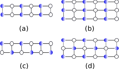
Figure 1: (a) and (b) show the rung occupied initial state on two- and three-leg ladders while (c) and (d) depict the diagonally occupied initial state.

For Hubbard chains, evidence for non-ergodic behavior has been found at strong disorder in numerical simulations.Mondaini and Rigol (2015) A non-ergodic phase was also found in the two-dimensional Anderson-Hubbard model with independent disorder for each spin species using a self-consistent perturbative approach.Lev and Reichman (2016) For coupled chains of non-interacting spinless fermions with independent potential disorder in each chain it has been found that interchain coupling can both strengthen or weaken Anderson localization, depending on the number of legs and the ratio of inter- to intrachain coupling.Weinmann and Evangelou (2014)

The purpose of this paper is to investigate quench dynamics in tight-binding models of fermionic chains with identical potential disorder for different initial states and interchain couplings, both in the non-interacting and in the interacting case. Our study relies on analytical arguments as well as on exact diagonalizations of finite systems. Our main results are: For the initial state used in the experiment of Ref. Bordia et al., 2016 (see Fig. 1(a,b)) we confirm that the dynamics in the non-interacting case is separable and completely independent of the coupling between the chains. The Anderson localized state is fully stable because perpendicular interchain couplings for this particular setup are ineffective. For generic interchain couplings and generic initial states, on the other hand, we find that the occupation imbalance does decay both in the Anderson and the MBL phase.

Our paper is organized as follows: In Sec. II we define the fermionic Hubbard models, initial states, and order parameters investigated. In Sec. III we obtain analytical results for the time dependence of the order parameters after a quench in the non-interacting, clean limit. Based on the initial state and the geometry of the interchain couplings we make several general observations in Sec. IV on whether or not the coupling between the chains will affect the dynamics. Specific cases of disordered free fermionic ladder models are considered in Sec. V while numerical results for interacting systems are provided in Sec. VI. In addition to the order parameters, we also consider the time evolution of the entanglement entropy of the ladder system, see Sec. VII. Finally, we summarize and conclude.

II Model

We consider a model of coupled fermionic Hubbard chains

$$H=-J\sum_{i,j=1;\sigma}^{L_{x}-1,L_{y}}(c^{\dagger}_{i,j,\sigma}c_{i+1,j,\sigma}+c^{\dagger}_{i+1,j,\sigma}c_{i,j,\sigma})$$ (1)

$$-J_{\perp}\sum_{i,j=1;\sigma}^{L_{x},L_{y}-1}(c^{\dagger}_{i,j,\sigma}c_{i,j+1,\sigma}+c^{\dagger}_{i,j+1,\sigma}c_{i,j,\sigma})$$

$$-J_{d}\sum_{i,j=1;\sigma}^{L_{x}-1,L_{y}-1}\!\!\!\!\!(c^{\dagger}_{i,j,\sigma}c_{i+1,j+1,\sigma}+c^{\dagger}_{i+1,j,\sigma}c_{i,j+1,\sigma}+h.c.)$$

$$+U\sum_{i,j=1}^{L_{x},L_{y}}\left(n_{i,j,\uparrow}n_{i,j,\downarrow}-\frac{1}{2}\right)+\sum_{i,j=1;\sigma}^{L_{x},L_{y}}D_{i}n_{i,j,\sigma}$$

with $L_{x}$ sites along the $x$ direction and $L_{y}$ sites along the $y$-direction. $c^{(\dagger)}_{i,j,\sigma}$ annihilates (creates) an electron with spin $\sigma=\uparrow,\downarrow$ at site $(i,j)$, and the local density operator is given by $n_{i,j,\sigma}=c^{\dagger}_{i,j,\sigma}c_{i,j,\sigma}$. $J$ is the hopping amplitude along the $x$-direction, $J_{\perp}$ the hopping amplitude along $y$, and $J_{d}$ a diagonal hopping amplitude. $U$ is the onsite Hubbard interaction. The random disorder potential $D_{i}$ only depends on the position along the $x$-direction. It is the same for all sites with the same index $j$. We assume open boundary conditions in both directions. In the numerical calculations we will set $J=1$.

We are interested in the non-equilibrium dynamics of the disordered fermionic Hubbard model (1) starting from a prepared initial product state. Following recent experiments on cold fermionic gases we consider, in particular, initial product states at quarter filling for chains with $L_{x}$ even. We concentrate on two initial states. The first one is given by

$$|\Psi_{1}\rangle=\prod_{i=1}^{L_{x}/2}\prod_{j=1}^{L_{y}}c^{\dagger}_{2i-1,j}|0\rangle\,.$$ (2)

In the following, we call this state the rung occupied state, see Fig. 1(a,b). The second initial state we will consider is the diagonally occupied state

$$|\Psi_{2}\rangle=\prod_{i=1}^{L_{x}/2}\prod_{j=1}^{L_{y}/2}c^{\dagger}_{2i,2j}c^{\dagger}_{2i-1,2j-1}|0\rangle\,,$$ (3)

depicted in Fig. 1(c,d). For free fermions the time evolution of the order parameter will not depend on the spin. For interacting fermions we consider the spin of the particles in the initial states above as being completely random.

For the initial state $|\Psi_{1}\rangle$ the order parameter is given by

$$I_{1}=\frac{2}{L_{x}L_{y}}\sum_{i,j}(-1)^{i+1}n_{ij}$$ (4)

while

$$I_{2}=\frac{2}{L_{x}L_{y}}\sum_{i,j}(-1)^{i+j}n_{ij}$$ (5)

is the order parameter for the initial state $|\Psi_{2}\rangle$. Here $n_{ij}=\sum_{\sigma}n_{ij\sigma}$. Both order parameters are normalized such that $\langle I_{1}(0)\rangle=\langle\Psi_{1}|I_{1}|\Psi_{1}\rangle=1$ and $\langle I_{2}(0)\rangle=\langle\Psi_{2}|I_{2}|\Psi_{2}\rangle=1$. In the following, we study the unitary time evolution of the order parameters $\langle I_{1,2}(t)\rangle$ under the Hamiltonian (1) for different sets of parameters.

III Free fermions in the clean limit

We start with the clean free fermion case $U=0$ and $D_{i}=0$. The Hamiltonian can then be diagonalized by Fourier transform and the time evolution of $\langle I_{1,2}(t)\rangle$ can be calculated analytically. The Fourier representation of the annihilation operator for open boundary conditions is given by

$$c_{ij\sigma}=\frac{2}{\sqrt{(L_{x}+1)(L_{y}+1)}}\sum_{k_{x},k_{y}}\sin k_{x}\sin k_{y}c_{k_{x},k_{y},\sigma}.$$ (6)

The wave vectors are quantized according $k_{x}=n\pi/(L_{x}+1)$ and $k_{y}=m\pi/(L_{y}+1)$ with $n=1,\cdots,L_{x}$; $m=1,\cdots,L_{y}$. Unitary time evolution results in

$$c_{k_{x},k_{y},\sigma}(t)=\exp(-\text{i}\varepsilon_{k_{x},k_{y},\sigma}t)c_{k_{x},k_{y},\sigma}$$ (7)

where the dispersion for model (1) reads

$$\varepsilon_{k_{x},k_{y}}=2J\cos k_{x}+2J_{\perp}\cos k_{y}+4J_{d}\cos k_{x}\cos k_{y}$$ (8)

and is independent of the spin index $\sigma$. Using the Fourier expansion (6) for the order parameter (4) we find

$$\langle I_{1}(t)\rangle = \frac{1}{L_{x}L_{y}}\sum_{n,m=1}^{L_{x},L_{y}}\exp[\text{i}(\varepsilon_{n,m}-\varepsilon_{L_{x}+1-n,m})]$$

$$= \frac{1}{L_{x}L_{y}}\sum_{k_{x},k_{y}}\exp\left[4\text{i}t\cos k_{x}\left(J+2J_{d}\cos k_{y}\right)\right]$$

$$\to \frac{1}{\pi}\int_{0}^{\pi}dk_{x}\exp[4\text{i}tJ\cos k_{x}]J_{0}(8J_{d}t\cos k_{x})$$

where we have taken the thermodynamic limit, $L_{x},L_{y}\to\infty$, in the last line with $J_{0}$ being the Bessel function of the first kind. Without the diagonal couplings ($J_{d}=0$) as in the experiment of Ref. Bordia et al., 2016 we find, in particular,

$$\langle I_{1}(t)\rangle=J_{0}(4Jt)\sim(2\pi Jt)^{-1/2}$$ (10)

in the thermodynamic limit while $\langle I_{1}(t)\rangle\sim(JJ_{d})^{-1/2}/t$ for $J_{d}\neq 0$.

Importantly, the result for the the initial state $|\Psi_{1}\rangle$ is always independent of the coupling in the transverse direction $J_{\perp}$. Without diagonal couplings we have a fine-tuned setup where $\langle I_{1}(t)\rangle$ is identical to the result for a single chain. While a generic coupling between the chains will typically lead to a faster dephasing and therefore to a faster decay of the order parameter this is not the case in such a fine-tuned setup.

For a finite number of legs one can also prevent the order parameter $\langle I_{1}(t)\rangle$ from decaying completely by fine-tuning the diagonal coupling $J_{d}$. This happens if for any of the allowed wave vectors $k^{(m)}_{y}=m\pi/(L_{y}+1)$ the diagonal coupling is chosen such that $J_{d}=-J/(2\cos k^{(m)}_{y})$. For an infinite two-leg ladder, for example, we find $\lim_{t\to\infty}\langle I_{1}(t)\rangle=1/2$ if $J_{d}=\pm J$ because $\cos k^{(m)}_{y}=\pm 1/2$ in this case.

The behavior of the order parameter (5) for the diagonal initial state (3), on the other hand, is very different. In this case we find

$$\langle I_{2}(t)\rangle=\frac{1}{L_{x}L_{y}}\sum_{k_{x},k_{y}}\exp\left[4it\left(J\cos k_{x}+J_{\perp}\cos k_{y}\right)\right]$$

$$\stackrel{{\scriptstyle L_{x},L_{y}\to\infty}}{{\to}}J_{0}(4Jt)J_{0}(4J_{\perp}t)\sim(JJ_{\perp})^{-1/2}(2\pi t)^{-1}$$ (11)

even without diagonal couplings. For the infinite two-dimensional lattice ($J_{\perp}\neq 0$, $J_{d}=0$) the order parameter is decaying $\sim 1/t$ for the diagonal initial state $|\Psi_{2}\rangle$ as compared to the $1/\sqrt{t}$ decay for the initial state $|\Psi_{1}\rangle$. The diagonally occupied state is thus a more generic initial state where a crossover from one- to two-dimensional behavior for free fermions does occur if the chains are coupled by a perpendicular hopping term.

IV General results for fermionic chains with identical disorder

In this section we want to provide some general arguments to show why the time evolution of the order parameter $\langle I_{1}(t)\rangle$ of the ladder system can be one-dimensional even in the presence of interchain couplings and disorder. We concentrate here on the system without the diagonal hopping terms ($J_{d}=0$) which will always make the system two-dimensional and which are not part of the experimental setup in Ref. Bordia et al., 2016.

First, we perform a Fourier transform along the direction of the interchain couplings $J_{\perp}$. Note that all sites for a given index $i$ along the $x$-direction have the same potential. The Hamiltonian (1) can then be written as $H=H_{J}+H_{J_{\perp}}+H_{D}=\sum_{i}h_{i}$ with

$$h_{i} = J\sum_{k_{y}}(c^{\dagger}_{i,k_{y}}c_{i+1,k_{y}}+h.c.)$$

$$+ 2J_{\perp}\sum_{k_{y}}\cos k_{y}n_{i,k_{y}}+D_{i}\sum_{k_{y}}n_{i,k_{y}}.$$

Similarly, we can write the order parameter as

$$I_{1}=\frac{2}{L_{x}L_{y}}\sum_{i,k_{y}}(-1)^{i+1}n_{i,k_{y}}.$$ (13)

In this representation it is immediately clear that $[H_{J_{\perp}},H_{J}]=[H_{J_{\perp}},H_{D}]=[H_{J_{\perp}},n_{i,k_{y}}]=0$ thus

$$c^{\dagger}_{i,k_{y}}c_{i,k_{y}}(t)=\text{e}^{-i(H_{J}+H_{D})t}c^{\dagger}_{i,k_{y}}c_{i,k_{y}}\text{e}^{i(H_{J}+H_{D})t}.$$ (14)

For free fermions $\langle I_{1}(t)\rangle$ is therefore independent of $J_{\perp}$ even in the presence of disorder. This order parameter will therefore always appear to indicate that the Anderson localized phase is stable against perpendicular interchain couplings.

If, on the other hand, diagonal hoppings are included then $H_{J_{d}}$ does not commute with $n_{i,k_{y}}$. In this generic situation the Anderson localized chain will be affected by the diagonal interchain couplings $J_{d}$. We analyze several examples in more detail in the next section. Similarly, introducing a Hubbard interaction $U$ implies that $H_{J_{\perp}}$ does not commute with the rest of the Hamiltonian anymore. On this level, the roles played by $H_{J_{d}}$ and $H_{U}$ are similar: both break the fine-tuned symmetry which make the disordered system behave completely one-dimensional even in the presence of couplings $J_{\perp}$ between the chains. Without the diagonal hopping terms the initial state $|\Psi_{1}\rangle$ together with the order parameter $\langle I_{1}(t)\rangle$ are thus not suitable to study the generic differences between Anderson and many-body localization in coupled chains with identical disorder.

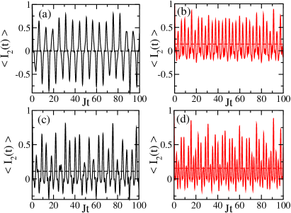
Figure 2: (Color online) $\langle I_{2}(t)\rangle$ for infinite binary disorder. Results for two-leg ladders (a,b) and three-leg ladders (c,d) with $200$ sites in the chain direction are presented. Interchain couplings are (a,c) $J_{\perp}=0.5$ and (b,d) $J_{\perp}=1$. Averages over $2000$ samples are shown. The dashed lines denote the long-time averages, see text.

V Free fermions with binary and box disorder

In this section we want to consider specific examples for the Hamiltonian (1) with $U=0$ and different types of disorder.

V.1 Free fermions with infinite binary disorder

Apart from the clean non-interacting case we can also study the case of binary disorder, $D_{i}=\pm D$, in the limit $D\to\infty$ analytically. We consider, in particular, a ladder with $L_{y}$ legs and $J_{d}=0$ in the limit $L_{x}\to\infty$. The infinite binary potential along the $x$-direction then splits the ladder system into decoupled finite clusters with equal potential. The disorder averaged time evolution of the system is then given by a sum of the time evolution of open clusters $I_{1,2}^{\ell}(t)$ with length $\ell$ along the $x$-direction and width $L_{y}$ weighted by their probability of occurence $p_{\ell}=\ell/2^{\ell+1}$ with $\sum_{\ell}p_{\ell}=1$ Andraschko et al. (2014). For infinite binary disorder the disorder average of the order parameters is therefore given by

$$\langle I_{1,2}^{D=\infty}(t)\rangle=\sum_{\ell=1}^{\infty}p_{\ell}\langle I_{1,2}^{\ell}(t)\rangle.$$ (15)

For the rung occupied state, $\langle I_{1}^{\ell}(t)\rangle$ does not depend on $J_{\perp}$. The result for $I_{1}^{D=\infty}(t)$ is therefore exactly the same as for a single chain. In particular, only clusters with $\ell$ odd give a contribution $\overline{I_{1}^{\ell\;\textrm{odd}}}=1/\ell$ to the time average so that $\overline{I_{1}^{D=\infty}}=\sum_{\ell\;\textrm{odd}}\frac{p_{\ell}}{\ell}=1/3$. There is no dephasing in the case of infinite binary disorder. $\langle I_{1}^{D=\infty}(t)\rangle$ does show persistent oscillations around the time average $\overline{I_{1}^{D=\infty}}=1/3$ Andraschko et al. (2014); Enss et al. (2017).

For the diagonally occupied state the situation is very different. Let us first consider the case of an even number of legs, i.e., $L_{y}$ even. In this case every decoupled cluster with equal potential of size $\ell\times L_{y}$ will have $\ell L_{y}/2$ fermions. For the generic case $J\neq J_{\perp}$ the order parameter $I_{2}^{\ell}(t)$ will then show persistent oscillations around zero for all cluster lengths $\ell$ resulting in $\overline{I_{2}^{D=\infty}}=0$. For $J=J_{\perp}$, on the other hand, clusters with length $\ell=n(L_{y}+1)-1$; $n=1,2,\cdots$ will give a contribution $\overline{I_{2}^{\ell}}=1/\ell$ to the time average so that $\overline{I_{2}^{D=\infty}}=\sum_{\ell}\frac{p_{\ell}}{\ell}=\sum_{n=1}^{\infty}2^{-n(L_{y}+1)}=1/(2^{L_{y}+1}-1)$. For $L_{y}$ odd and $J\neq J_{\perp}$ all clusters with odd length $\ell$ will give a contribution $1/(L_{y}\ell)$ so that $\overline{I_{2}^{D=\infty}}=1/(3L_{y})$. For $J=J_{\perp}$ and $L_{y}$ odd, clusters of length $\ell=n(L_{y}+1)-1$, $n=1,2,\cdots$ will give a $1/\ell$ contribution to the time average while all other odd clusters will contribute $1/(L_{y}\ell)$ giving rise to a time average

$$\overline{I_{2}^{D=\infty}}=\frac{1}{3L_{y}}+\frac{1-1/L_{y}}{2^{L_{y}+1}-1}.$$ (16)

In Fig. 2 these analytically obtained long-time averages are compared to numerical data. For the two-leg ladder with $J_{\perp}=0.5J$, see Fig. 2(a), the long-time average is zero while for $J_{\perp}=J$, see Fig. 2(b), we have $\overline{I_{2}}=1/7$. For the three-leg ladder we find, on the other hand, $\overline{I_{2}}=1/9$ and $\overline{I_{2}}=7/45$, respectively.

To summarize, there is an interesting even/odd effect for the diagonally occupied state with $\overline{I_{2}^{D=\infty}}=0$ for $L_{y}$ even and $\overline{I_{2}^{D=\infty}}=\frac{1}{3L_{y}}$ for a generic interchain coupling $J_{\perp}\neq J$. In the following subsection we will see that these even/odd effects do persist for finite box disorder.

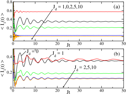
Figure 3: (Color online) $\langle I_{1}(t)\rangle$ for (a) two-leg ladders and (b) three-leg ladders with $200$ sites along the chain direction, box disorder $D=5$ and different diagonal couplings $J_{d}$ as indicated. The results are independent of the perpendicular interchain coupling $J_{\perp}$. Averages over $1000$ samples are shown with statistical errors of the order of the line width.

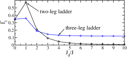
Figure 4: (Color online) Long-time averages $\overline{I_{1}}$ for the data shown in Fig. 3. For the two-leg ladder the data are consistent with a power-law decay to zero for $J_{d}\to\infty$ while a power-law fit yields $\overline{I_{1}}(J_{d}\to\infty)\approx 0.119$ for the three-leg ladder.

V.2 Free fermions with box disorder

Here we want to present numerical results for non-interacting ladders with disorder drawn from a box distribution $D_{i}\in[-D,D]$. Because the system is non-interacting, calculating the order parameters $\langle I_{1,2}(t)\rangle$ reduces to an effective one-particle problem which can be solved numerically for large system sizes. We start from the initial $L_{x}L_{y}/2$ one-particle states in position representation and time evolve each of these states using the Hamiltonian (1) with $U=0$. The order parameters are then simply given by the sum of the order parameters for each one particle wave function. We have checked that the numerical data agree with the analytical solutions in Sec. III for the clean case and that $\langle I_{1}(t)\rangle$ is indeed independent of $J_{\perp}$ for all disorder strengths.

We start by presenting data in Fig. 3(a) for the time evolution in two-leg ladders prepared in the rung occupied initial state. As discussed in section Sec. IV the results are independent of $J_{\perp}$. While the order parameter is increased for $J_{d}=J$, stronger diagonal couplings lead to a decrease and the data are consistent with $\overline{I_{1}}\to 0$ for $J_{d}\to\infty$, see Fig. 4. In Fig. 3(b) data for the same parameters but for three-leg ladders are shown. The results are quite different from the two-leg case. While the results are again independent of $J_{\perp}$, we now find that the long-time average $\overline{I_{1}}$ remains non-zero even for strong interchain couplings $J_{d}/J\gg 1$, see Fig. 4. The long-time behavior is thus quite different for ladders with an even or an odd number of legs. Similar to the case of infinite binary disorder we expect that for ladders with an odd number of legs the long-time average $\overline{I_{1}}$ decreases with the number of legs. Coupling an infinite number of Anderson localized chains with identical disorder in a generic way will thus lead to a complete destruction of the order parameter.

Next, we present data for the diagonally occupied initial state in Fig. 5.

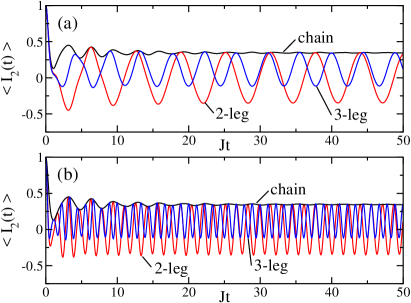
Figure 5: (Color online) $\langle I_{2}(t)\rangle$ for a chain, a two-leg, and a three-leg ladder with $200$ sites along the chain direction and $D=5$. (a) $J_{\perp}=0.5$, and (b) $J_{\perp}=2$. Averages over $1000$ samples are shown. $\overline{I_{2}}\neq 0$ for the single chain and the three-leg ladder while $\overline{I_{2}}=0$ for the two-leg ladder.

The results are qualitatively similar to the case of infinite binary disorder solved analytically in the previous section. In particular, we find that for generic interchain couplings $J_{\perp}$ the long-time average $\overline{I_{2}}$ is zero for an even number of legs while it is non-zero for an odd number of legs.

VI Interacting ladder models

We now turn to a numerical study of the interacting case. Here we are limited to the exact diagonalization of rather small two-leg ladders. While the system sizes could, in principle, be increased the substantial number of samples required to obtain disorder averages with small statistical errors is a further limiting factor in practice. Nevertheless, even these small systems show behavior which is qualitatively consistent with the experimental results in Ref. Bordia et al., 2016.

VI.1 Spinful fermions

We concentrate first on spinful fermions on a two-leg ladder with onsite Hubbard interaction $U$. For a $4\times 2$ ladder with $n_{\uparrow}=n_{\downarrow}=2$ the Hilbert space has dimension ${\binom{8}{2}}^{2}=784$. We find that in the interacting case a much larger number of samples than in the non-interacting case is required (by at least a factor of $10$) to obtain the same accuracy for the disorder average. For a $4\times 2$ ladder this is still easily achievable while already for a $6\times 2$ ladder with $n_{\uparrow}=n_{\downarrow}=3$ the Hilbert space dimension is ${\binom{12}{3}}^{2}=48400$, and an enormous amount of computing resources would be required. Instead, we will also present results for a $6\times 2$ ladder with $n_{\uparrow}=4$ and $n_{\downarrow}=2$ with Hilbert space dimension ${\binom{12}{2}}{\binom{12}{4}}=32670$.

In Fig. 6 the order parameter $\langle I_{1}(t)\rangle$ for the $4\times 2$ ladder is shown for different interaction strengths $U/J$.

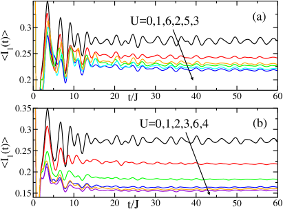
Figure 6: (Color online) $\langle I_{1}(t)\rangle$ for a $4\times 2$ ladder of spinful fermions with disorder $D=2.5$. Averages over $200\,000$ samples are shown. (a) $J_{\perp}=0.1$, and (b) $J_{\perp}=1$. The Hubbard interactions $U$ are indicated.

Both for weak and for strong interchain coupling, increasing the Hubbard interaction initially leads to a decrease of the long time average $\overline{I_{1}}$ with a minimum at $|U|/J\sim 4-5$, see Fig. 7(a).

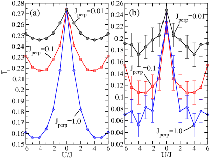
Figure 7: (Color online) Long-time average $\overline{I_{1}}$ at disorder $D=2.5$ for (a) a $4\times 2$ ladder with $n_{\uparrow}=n_{\downarrow}=2$ for $200\,000$ samples, see Fig. 6, and (b) a $6\times 2$ ladder with $n_{\uparrow}=4$ and $n_{\downarrow}=2$ for $400$ samples. Note that the dependence on $|U|/J$ is non-monotonic.

For even larger interaction strengths the long-time average increases again leading to a characteristic shape of the imbalance versus $|U|/J$ curve qualitatively consistent with the experimental data obtained in Ref. Bordia et al., 2016. The same is true for the $6\times 2$ ladder, see Fig. 7(b), although the small number of samples we have simulated leads to relatively large error bars. Note that the arguments presented in Ref. Enss and Sirker, 2012 for the $U\to-U$ symmetry in such quenches for clean Hubbard models remain valid even if potential disorder is included. The sign of $U$ does not affect the quench dynamics.

Results for the diagonal initial state $|\Psi_{2}\rangle$ are shown in Fig. 8.

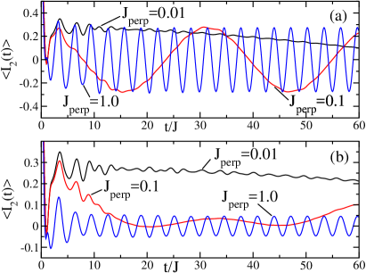
Figure 8: (Color online) $\langle I_{2}(t)\rangle$ for a $4\times 2$ ladder of spinful fermions with disorder $D=2.5$. Averages over $500\,000$ samples are shown for (a) $U=0$, and (b) $U=4$. The interchain coupling $J_{\perp}$ is indicated on the graph. $\langle I_{2}(t)\rangle$ for $J_{\perp}=0.1$ in (b) also starts to oscillate around zero for longer times (data not shown).

For $U=0$, see Fig. 8(a), we obtain results for the $4\times 2$ ladder which show qualitatively the same behavior as the ones already presented in Fig. 5 for much larger ladders. $\langle I_{2}(t)\rangle$ for $J_{\perp}\neq 0$ oscillates around zero with $J_{\perp}$ determining the oscillation frequency. While the oscillation amplitude around zero is modified for $U=4$, see Fig. 8(b), there is otherwise no qualitative difference between the non-interacting and the interacting case. For a given coupling strength $J_{\perp}$ the time scale for the initial decay of $\langle I_{2}(t)\rangle$ is of the same order. For interchain coupling $J_{\perp}=1$ we observe, in particular, an almost complete decay of the order parameter on a time scale of order $J$ in both cases.

VI.2 Spinless fermions

While our numerical results for spinful $4\times 2$ and $6\times 2$ ladders demonstrate behavior which is qualitatively consistent with the experimental data, the system sizes are quite small. To corroborate these results we thus also consider the case of spinless fermionic two-leg ladders where larger system sizes can be simulated. Instead of an onsite Hubbard interaction $U$ we now introduce a nearest-neighbor interaction

$$H_{V}=V\sum_{i}\left(n_{i,1}n_{i,2}+n_{i,1}n_{i+1,1}+n_{i,2}n_{i+1,2}\right).$$ (17)

Results for a $8\times 2$ ladder with $8$ fermions are shown in Fig. 9. As in the spinful case, the dynamics for $V=0$ is one-dimensional and completely independent of the strength of the interchain coupling $J_{\perp}$: the results for $V=0$ in Fig. 9(a) and Fig. 9(b) are identical.

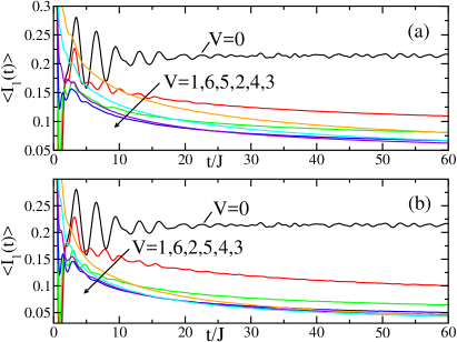
Figure 9: (Color online) $\langle I_{1}(t)\rangle$ for a $8\times 2$ ladder of spinless fermions with disorder $D=2.5$. $2000$ to $20\,000$ samples are used. (a) $J_{\perp}=0.1$, and (b) $J_{\perp}=1$. The nearest-neighbor interactions $V$ are indicated.

Adding nearest-neighbor interactions leads to a strong reduction of the order parameter both for weak and strong hopping between the chains.

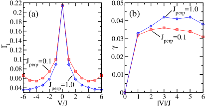
Figure 10: (Color online) Fitting the data in Fig. 9 according to $\langle I_{1}(t)\rangle=\overline{I_{1}}+a\exp(-\gamma t)$ for $t>30$ allows to extract estimates for the long-time average $\overline{I_{1}}$ shown in panel (a) and the decay rate $\gamma$ shown in panel (b).

The decay of the order parameter at long times in the interacting case seems to be well described by an exponential. The long-time average and the decay rate extracted from exponential fits are shown in Fig. 10. The results show that both the long-time average $\overline{I_{1}}$ and the decay rate $\gamma$ do depend on the strength of $J_{\perp}$ albeit rather weakly. For weak interchain coupling $J_{\perp}=0.1$ we observe a non-monotonic dependence of $\overline{I_{1}}$ on the interaction strength similar to the spinful case.

VII Entanglement entropy

In this final section we want to briefly discuss the entanglement properties of fermionic ladders. We consider ladders where the chains contain an even number of sites and cut the ladder into two equal halfs, $A$ and $B$, perpendicular to the chain direction. The von Neumann entanglement entropy is then defined as

$$S_{\textrm{ent}}(t)=-\textrm{tr}\,\rho_{A}(t)\ln\rho_{A}(t)$$ (18)

where $\rho_{A}(t)=\textrm{tr}_{B}|\Psi_{i}(t)\rangle\langle\Psi_{i}(t)|$ is the reduced density matrix of segment $A$.

If we start from one of the product states $|\Psi_{1,2}\rangle$ then the entanglement entropy for a clean ladder grows linearly in time before saturating at a constant for times $t>L_{x}/(2v)$ where $L_{x}/2$ is the length of the segment and $v\sim 2J$ the velocity of excitations.Calabrese and Cardy (2009) The entanglement entropy per chain, $S_{\textrm{ent}}(t)/L_{y}$, in the clean case is independent of the number of legs $L_{y}$ and independent of the coupling $J_{\perp}$ between the ladders for $J_{d}=0$. For spinless fermions we find, in particular, that $S_{\textrm{ent}}(t)/L_{y}\sim 0.88t$ for $t<L_{x}/(2v)$ consistent with the results for a single chain.Zhao et al. (2016) Similar to the order parameter $\langle I_{1}(t)\rangle$ the entanglement entropy $S_{\textrm{ent}}(t)$ for the rung occupied initial state remains independent of the interchain coupling $J_{\perp}$ in the non-interacting case even if we include disorder. Without interactions or diagonal couplings, $S_{\textrm{ent}}(t)$ of a ladder prepared in the rung occupied initial state is simply $L_{y}$ times the entanglement entropy of a single chain. This demonstrates further that the stability of the Anderson localized state cannot be investigated in this setup.

One way to allow for dynamics which involves the full ladder is to include diagonal couplings. As demonstrated in Fig. 11, $S_{\textrm{ent}}(t)$ is then no longer simply given by $L_{y}$ times the entanglement entropy of a single chain but rather grows more rapidly with the number of legs as expected when moving towards a two-dimensional system.

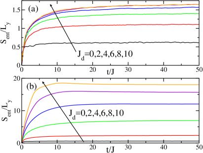
Figure 11: (Color online) Entanglement entropy per chain of free spinless fermions starting from the rung initial state with disorder $D=2.5$ and different $J_{d}$ for (a) a two-leg ladder, and (b) a three-leg ladder. The results are independent of $J_{\perp}$. The length of both ladders is $200$ sites along the chain direction; averages over $2000$ samples are shown.

The entanglement entropy at long times increases monotonically with $J_{d}$ up to a maximum value. The maximal value is determined by the smaller of the two relevant length scales: the localization length and the block size.

Another way of breaking the one-dimensionality of the dynamics is to include interactions. As demonstrated in Fig. 12 the entanglement entropy then depends on the strength of the interchain coupling $J_{\perp}$ even without the diagonal couplings.

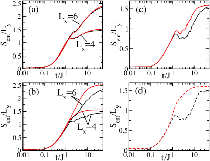
Figure 12: (Color online) Entanglement entropy per chain for interacting spinful fermions on a $4\times 2$ ladder with $n_{\uparrow}=n_{\downarrow}=2$ ($4000$ samples) and a $6\times 2$ ladder ($400$ samples) with $n_{\uparrow}=4$, $n_{\downarrow}=2$. The interchain couplings are $J_{\perp}=0.1$ (black lines) and $J_{\perp}=1$ (red lines). Left panels: rung initial state, right panels: diagonal initial state. (a,c) $U=1$ and (b,d) $U=6$.

For spin chains it has been shown that the entanglement entropy increases logarithmically in the many-body localized phase.Žnidarič et al. (2008); Bardarson et al. (2012) While some of the data in Fig. 12 might be hinting at such a scaling, the system sizes are too small to observe scaling over a large time interval. We also note that it has recently been argued—based on numerical data—that the entanglement growth in a Hubbard chain with potential disorder does not grow logarithmically but rather follows a power law with an exponent much smaller than $1$.Prelovšek et al. (2016)

In addition to the spinful case we therefore also consider the spinless case, see Fig. 13.

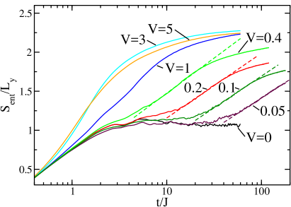
Figure 13: (Color online) Entanglement entropy per chain for interacting spinless fermions on a $8\times 2$ ladder with box disorder $D=2.5$ prepared in the rung initial state. Results for $1000$ samples with $J_{\perp}=1$ are shown. The dashed lines are logarithmic fits.

In this case we do see clear signatures of a logarithmic scaling for small interactions $V$ which seem to indicate that the ladder for $D=2.5$ is already in the many-body localized phase. Determining the phase diagram of the ladder as a function of disorder strength $D$ and interaction $V$ is difficult using exact diagonalization because of the limited system sizes accessible and is beyond the scope of this paper.

VIII Conclusions

We have studied non-equilibrium dynamics and localization phenomena in fermionic Hubbard ladders with identical disorder along the chain direction using analytical calculations in limiting cases as well as exact diagonalizations. In the free fermion case we confirm that a perpendicular coupling between the chains does not affect the dynamics for an initial state where all even sites on the chains are occupied by one fermion while all odd sites are empty (rung occupied state). Anderson localization in the chains appears to be stable in such a setup simply because turning on the perpendicular interchain couplings does not affect the dynamics at all.

In order to study the differences in the response to interchain couplings between an Anderson and a many-body localized system in a non-trivial setup, we considered to either modify the initial state, or to allow for additional diagonal hoppings between the chains.

For the modified initial state—where even sites are occupied by one fermion on even legs and odd sites on odd legs (diagonal occupied state)—we did not find any qualitative difference between the Anderson and the many-body localized state. In both cases interchain coupling leads to a complete decay of the order parameter for a two-leg ladder. At least for small systems there is also no discernible difference in the time scales for the decay of the order parameter between the interacting and the non-interacting model.

Similarly, we found that the order parameter for the rung occupied state does decay also in the non-interacting case if we allow for diagonal hoppings which truly couple the chains. Qualitatively, there is again no difference between the Anderson and the many-body localized case: in both cases the initial order is unstable to generic couplings between the chains.

While a more detailed analysis of the long-time average of the order parameter, the decay time, and of the entanglement entropy does reveal quantitative differences between the non-interacting and the interacting case, coupling chains with identical disorder in a generic way does not appear to be a ’smoking gun’ experiment to distinguish Anderson and many-body localized systems.